Yet another introduction to linear dynamical systems control: From identification and approximation to digital control

Abstract

This report aims at presenting (yet) a(nother) methodology to design and implement a linear controller for linear dynamical systems on practical applications. The specificity of this report is that authors try to cover (obviously in a non exhaustive way) a wide range of control engineering fields. Indeed, the main purpose is to give a quick overview of standard control engineer approaches to non familiar readers. More specifically, using a simple toy example, we discuss the main steps control engineers usually follow. Namely, (i) the excitation signals construction, (ii) the (continuous-time) linear model construction and approximation, (iii) the (continuous-time) control design, and finally, (iv) its time-domain discretisation and control signal modulation in view of practical implementation. This report is clearly user-oriented and thus focuses on practical aspects (using Matlab code) rather than on theoretical ones, let to the reader’s curiosity with few but relevant references.

1 Motivation and framework

As stated in the abstract, we will consider dynamical systems and control design through the lens of continuous-time linear functions. Readers should keep in mind that nonlinear systems theory and methods exist but, to the authors feeling, may be viewed as more tedious to apply in a systematic way. The discrete-time (or sampled-time) will be briefly discussed in the last section.

1.1 Assumption and framework

Generally speaking, this report considers finite order Multiple Input Multiple Outputs (MIMO ) $n_{u}$ inputs $n_{y}$ outputs Linear Time Invariant (LTI ) dynamical systems denoted $\mathbf{\Sigma}$ described by a complex, or frequency-domain, transfer function $\mathbf{H}$,

$$\mathbf{H}:\mathds{C}\rightarrow\mathds{C}^{n_{y}\times n_{u}},$$ (1)

which maps linearly the inputs $\mathbf{u}$ to the outputs $\mathbf{y}$ as,

$$\begin{array}[]{rcl}\mathbf{y}(s)&=&\mathbf{H}(s)\mathbf{u}(s)\\ \end{array}$$ (2)

This mapping can also be seen from a time-domain perspective as a set of first-order Differential Algebraic Equations (DAE ) described by a descriptor realisation $\mathcal{S}$,

$${E}\dot{\mathbf{x}}(t)={A}\mathbf{x}(t)+{B}\mathbf{u}(t)\text{ and }\mathbf{y}(t)={C}\mathbf{x}(t),$$ (3)

where $\mathbf{x}(t)\in\mathds{R}^{n}$ denotes the internal variables (the state variables if ${E}$ is invertible), $\mathbf{u}(t)\in\mathds{R}^{n_{u}}$ and $\mathbf{y}(t)\in\mathds{R}^{n_{y}}$ are the input and output signals, respectively, and ${E},{A}\in\mathbb{R}^{n\times n}$, ${B}\in\mathbb{R}^{n\times n_{u}}$ and ${C}\in\mathbb{R}^{n_{y}\times n}$ are constant matrices. It is common to name $({E},{A})$ as the dynamical matrices, while ${B}$ and ${C}$ are the input and output ones.

The external, frequency-domain description of $\mathbf{\Sigma}$ is related its internal, time-domain description by the expression of its transfer function $\mathbf{H}$ w.r.t. the matrices of the realisation $\mathcal{S}$ when the pencil $({E},{A})$ is regular,

$$\mathbf{H}(s)={C}\left(s{E}-{A}\right)^{-1}{B}.$$ (4)

Figure 1 provides a graphical view of the system $\mathbf{\Sigma}$, as well as its (i) external representation $\mathbf{H}$ from $\mathbf{u}$ to $\mathbf{y}$ and (ii) its internal view $\mathcal{S}$, including $\mathbf{x}$.

Figure 1: Graphical view of a (linear) dynamical system with inputs $\mathbf{u}$, outputs $\mathbf{y}$ and internal variables $\mathbf{x}$.

Readers may note that unlike most control textbooks, the internal representation $\eqref{eq:S}$ does not contain any ${D}$ term in the output while there is a matrix ${E}$ in the dynamical equation. It turns out that the description (3) can encompass the ${D}$ matrix and actually allows to describe a wider class of systems (see e.g. [1, 2] for interesting discussion on this topic).

As schematised in Figure 1, continuous MIMO LTI dynamical model (or system) $\mathbf{\Sigma}$ defines an ”input-output” map associating an input signal $\mathbf{u}$ to an output one $\mathbf{y}$ by means of the convolution operation,

$$\mathbf{y}(t)=\mathbf{h}(t)*\mathbf{u}(t)=\int_{-\infty}^{\infty}\mathbf{h}(t-\tau)\mathbf{u}(\tau)d\tau,$$

where $\mathbf{h}(t)$ is the impulse response of the system $\mathbf{\Sigma}$. It is (strictly) causal if and only if $\mathbf{h}(t)=0$ for ($t\leq 0$) $t<0$ (in this case ${E}$ is full rank). Taking the Laplace transform of this input-ouput mapping leads to equation (2) where $\mathbf{u}(s)$ and $\mathbf{y}(s)$ are the Laplace transform of $\mathbf{u}(t)$ and $\mathbf{y}(t)$, respectively. An LTI system $\mathbf{\Sigma}$ is said to be stable if and only if its transfer function $\mathbf{H}$ is bounded and analytic on $\mathds{C}_{+}$, i.e. it has no singularities on the closed right half-plane. Conversely, it is said to be anti-stable if and only if its transfer function is bounded and analytic on $\mathds{C}_{-}$ (see also [5] or Chapter 2 of [8] for more details). When $\mathbf{H}$ is associated with a first order descriptor realisation $\mathcal{S}:({E},{A},{B},{C})$ as in (3), it is rational and has a finite number of singularities called poles or (eigen-)modes of the system. These poles are the singularities of the $({E},{A})$ pencil $\forall\lambda\in\mathds{C}$ as $\mathbf{det}({A}-\lambda{E})$. This pencil is regular if at least there exist $\lambda$ such that $\mathbf{det}({A}-\lambda{E})\neq 0$. We call $\lambda$ an eigenvalue of $({E},{A})$ if $\mathbf{det}({A}-\lambda{E})=0$.

Based on this fairly general introduction of variables and elements of linear dynamical systems theory, the remainder of this tutorial is restricted to a simple example.

1.2 Considered use-case

For didactical purpose, the following assumption will be considered: the system $\mathbf{\Sigma}$ is a (i) stable (ii) Single Input Single Output (SISO ), i.e. $n_{u}=n_{y}=1$ and (iii) described by strictly proper and rational function (${E}$ is full rank and thus does not admit a direct feed-through term). Authors stress that while assumptions (i)-(ii) are chosen for educational purpose, assumption (iii) is also related to more complex issues omitted here and where details may be found e.g. in [9, 2].

In this report, a simple yet interesting second order LTI SISO system $\mathbf{\Sigma}$ use-case is considered. Let us assume that the system $\mathbf{\Sigma}$ to be studied is described by the (unknown) following transfer function $\mathbf{G}$ and realisation $\mathcal{S}$,

$$\begin{array}[]{rcl}\mathbf{y}(s)&=&\mathbf{G}(s)\mathbf{u}(s)\\ &=&\dfrac{k}{s^{2}/w_{0}^{2}+2ds/w_{0}+1}\mathbf{u}(s)\\ &=&\underbrace{\left[\begin{array}[]{cc}0&w_{0}^{2}\end{array}\right]}_{{C}}\underbrace{\left(sI_{2}-\left[\begin{array}[]{cc}-dw_{0}&w_{0}\sqrt{1-d^{2}}\\ -w_{0}\sqrt{1-d^{2}}&-dw_{0}\end{array}\right]\right)^{-1}}_{\left(s{E}-{A}\right)^{-1}}\underbrace{\left[\begin{array}[]{c}k/w_{0}\sqrt{1-d^{2}}\\ 0\end{array}\right]}_{{B}},\end{array}$$ (5)

where $d=0.2$ is the damping ratio (note that it is standard to consider $0<d<1$), $\omega_{0}=\sqrt{\omega_{1}^{2}+d^{2}}$rad/s (where $\omega_{1}=10$rad/s is the cut-off frequency) and $k$ is the static gain. Such a model represents a simple weakly damped ($d<\sqrt{2}/2$) second order model system with cut-off dynamic at $\omega_{1}$. The corresponding Bode diagram, representing the response of $\mathbf{G}(s)$ for varying values of $s=\imath\omega$, where $\omega\in\mathds{R}$ (i.e. the response of the complex function along the imaginary axis $\imath\mathds{R}$) is given in the following Figure 2, where the gain is shown on the top frame while the phase on the bottom one. Note that the gain exhibits a bump at $f_{1}=\omega_{1}/(2\pi)$ due to the low damping $d$ value, a static value above 0dB and a roll-off below $\omega_{1}$. Regarding the phase, a sharp drop of $-\pi$ at $f_{1}$ is also observed (note that a $x$-axis log-scale and gain $y$-axis in dB are standardly used).

Figure 2: Frequency response gain (top) and phase (bottom) of the example model $\mathbf{G}$ (G in the code).

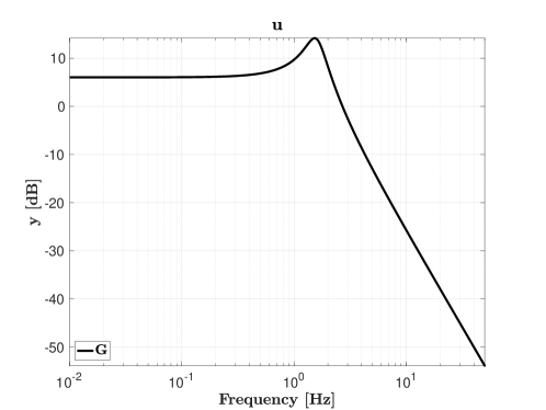
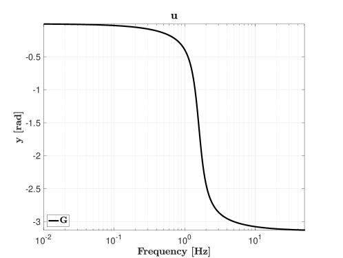
The associated realisation is represented by two first order ODE indicating that two storage states are embedded in the system. Note that the choice of the $({E},{A},{B},{C})$ quadruple, being constant linear matrices in $(\mathds{R}^{n\times n},\mathds{R}^{n\times n},\mathds{R}^{n\times n_{u}},\mathds{R}^{n_{y}\times n})$, has been done among an infinite set of possibilities. Indeed, by considering any full-rank matrix $V\in\mathds{R}^{n\times n}$, the projected realisation $(V^{-1}{E}V,V^{-1}{A}V,V^{-1}{B},{C}V)$ leads to the same transfer function, and thus input output relation. The following Matlab code provides a way to define such a system.

⬇

% Model description as Transfer Function and State-Space

d = .2;

k = 2;

w1 = 10; w0 = sqrt(w1^2+d^2);

G = tf(k,[1/w0^2 2*d/w0 1]); G.InputName = ’u’; G.OutputName = ’y’;

Gss = ss([-d*w0 w0*sqrt(1-d^2); -w0*sqrt(1-d^2) -d*w0],[0; w0^2],[k/(w0*sqrt(1-d^2)) 0],0);

./code/start.m

Listing 1: Example file start2ndOrder.m: $\mathbf{G}$ model description.

1.3 Reader target and some advertisement

As stated in the abstract, this reports tries to cover a wide spectrum of linear signal processing and control theory aspects, and reader should be aware that the present document is not complete at all and should be amended and enhanced in many ways. It is principally meant at providing very basic elements that may be considered as control starting points for non experts people. The report is centred on the engineering soundness and thus focuses on the practical aspects rather than on the theoretical ones, even if authors try paying attention in giving accurate explanations, especially in the transitions from a part to an other.

1.4 Report structure

The present report follows the - control engineer-like - classical flow: Section 2 exposes some elements about the generation of exciting signals, i.e. signals that can be used for model construction. Based on these excitation signals and the resulting measured outputs, Section 3 then explains how an (approximate) LTI model ($\mathbf{\hat{H}}$) $\mathbf{H}$ of the system $\mathbf{\Sigma}$ can be constructed. Hopefully, ($\mathbf{\hat{H}}$) $\mathbf{H}$ should be identical to $\mathbf{G}$ as defined in (5). As it is now well admitted that it is an efficient and versatile tool for linear model approximation and reduction, the lens of the model approximation and interpolatory framework is chosen to be the identification and approximation main tool. Section 4 then describes a model-based continuous-time linear controller $\mathbf{K}$ design approach, using the ${\mathcal{H}_{\infty}}$-norm minimisation criteria. Again, such a choice has been done purposely considering the author’s background in control theory, but (m)any other approach can be used and be somehow approached with the same philosophy. One major benefit of the ${\mathcal{H}_{\infty}}$ approach is that it is relatively simple to understand and the available tools for optimising the control structure and gains are powerful, very versatile and accessible to many engineers. This section closes with the discretisation $\mathbf{K}_{z}$ of the aforementioned controller and provides preliminary comments on the hybrid interconnection (continuous/sampled). Section 5 present an issue encountered by many practitioners, namely the modulation of the control signal to tackle the case where actuators are pulsed (on/off). This modulation choice is done considering the numerous discussions authors got from practitioners and therefore seems of interest. As it is a fairly complex point, this last section is mainly based on simulations and the discussion remains preliminary. Conclusions and some questions are discussed in Section 6.

2 Identification signals

The main aim of identification signals is to generate an input signal exciting enough to enable an accurate identification of the underlying system, here represented by a linear second order model $\mathbf{G}$. Such a signal should then satisfy some hypothesis such as applicability, be exciting enough and simple. In general for linear systems, the frequencies of identification signal should excite all the relevant frequencies of the system. Once again, as it is quite far from the main expertise of the authors, reader should take the following section as a naive, but simple to reproduce, approach.

2.1 Reminders on Fourier transform

As most of the report is based on the frequency-domain representation of dynamical systems, let us first recall some basic elements on Fourier transform. Given signal $\mathbf{x}(t)$ the Fourier transform reads

$$\begin{array}[]{rcl}\tilde{\mathbf{x}}(f)=\textbf{{TF}}\left(\mathbf{x}(t)\right)&=&\displaystyle\int_{\mathds{R}}\mathbf{x}(t)e^{-2\pi\imath ft}dt\\ &=&\left\lvert\tilde{\mathbf{x}}(f)\right\rvert e^{\imath\phi(f)},\end{array}$$ (6)

where the complex variable $\tilde{\mathbf{x}}(f)$ is the spectrum of $\mathbf{x}(t)$ and where $\phi(f)$ denotes the argument of $\tilde{\mathbf{x}}(f)$. The time $t$ and frequency $f$ are the variables embedded in the transform. Importantly, the Fourier transform exists for any finite energy signals $\mathbf{x}(t)$ (it is a sufficient condition). One may note that the dual inverse Fourier operator exists. As a remark, one can remember that signals with small support has a large spectrum. As an illustration, given the rectangle function (note tat such shape has some interest in application, as shown at the end of this report)

$$\mathbf{x}(t)=\textbf{rect}_{T}(t/T)\left\{\begin{array}[]{ll}1&\text{, $\forall t\in[-T/2,T/2]$}\\ 0&\text{, elsewhere}\end{array}\right.$$ (7)

the corresponding Fourier transform reads

$$\tilde{\mathbf{x}}(f)=\dfrac{\sin(\pi fT)}{\pi f}=T\mathbf{sinc}(\pi Tf).$$ (8)

2.2 Some exciting signal

Back to our problem, the first objective of a control engineer is to construct exciting signal that will allow us for constructing a linear model $\mathbf{H}$ of the system $\mathbf{\Sigma}$, here being $\mathbf{G}$ but considered as unknown. There exists a lot of identification signals and it is actually a complete research field in systems theory, but for simplicity, among them, one can mention the (fairly standard) following ones:

• Pseudo random binary signal (PRBS). It consists in on/off like signals used as input. The idea is to define a "random" sequence of these signals in order to emulate a white noise. The longest duration should last enough to reach steady state output and the shortest should be short enough to excite frequencies above the cut-off one of the system. The Fourier transform of such signal should be constant over frequencies. Note that for the same reason as the one mentioned above in the rectangular signal, to be a white (more accurately pink) noise, a whitening filter should be combined to the random rectangular sequence, avoiding the frequency-domain zeros embedded in the $\mathbf{sinc}$ function.

• Frequency chirp signal. It consists in a cosine-like function that sweeps from a low frequency up to a high one. The signal should sweep sufficiently slowly to excite all frequencies. Similarly to the above random binary signal, the Fourier transform covers all frequencies in the interval of the sweep. An illustration of such a signal and its response when fed in the example use case $\mathbf{G}$ is given in Figure 3.

  

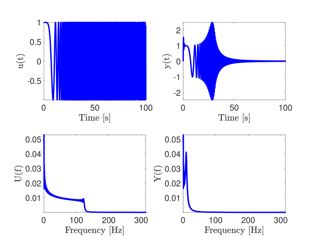
  Figure 3: Chirp (frequency sweep) signal. Top: time-domain input signal $\mathbf{u}(t)$ (left) and output measurement $\mathbf{y}(t)$ (right). Bottom: frequency-domain corresponding signals $\tilde{\mathbf{u}}(f)$ and $\tilde{\mathbf{y}}(f)$, respectively.

• Impulse signal. It consists in injecting a causal Dirac input, denoted $\delta(t)$. Theoretically, a Dirac signal reads

  $$\delta(t)=\left\{\begin{array}[]{ll}1&\text{, $t=0$}\\ 0&\text{, elsewhere}\end{array}\right..$$ (9)

  It naturally translates as

  $$\tilde{\mathbf{x}}(t)=\textbf{{TF}}\left(\mathbf{x}(t)\right)=\int_{-\infty}^{+\infty}\delta(t)dt=1.$$ (10)

  The Fourier transform of the Dirac function is a unitary gain over all frequencies. Thus, Dirac functions encompasses all frequencies (note that a continuous signal contains the frequency zero, only). In practical signal processing, it is used for frequency modulation. In practice, such a signal is impossible to generate and a rectangular signal with small width is preferred. The resulting spectrum is generally a cardinal sine like and thus also a pink noise. An illustration of such a signal and its response when fed in the example use case $\mathbf{G}$ is given in Figure 4.

  

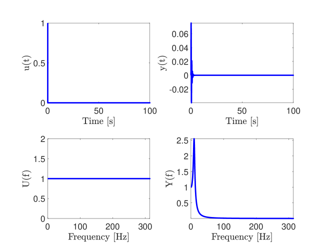
  Figure 4: Impulse signal. Top: time-domain input signal $\mathbf{u}(t)$ (left) and output measurement $\mathbf{y}(t)$ (right). Bottom: frequency-domain corresponding signals $\tilde{\mathbf{u}}(f)$ and $\tilde{\mathbf{y}}(f)$, respectively.

Note that as we consider linear systems only, one single amplitude is enough for identification. Obviously, in nonlinear cases, this statement is not true anymore. From the rest of the report, we will consider results obtained when using the second exciting signal, i.e. the frequency sweep one. The signals are obtained using the following Matlab code with inputExcitation=’chirp’.

⬇

switch inputExcitation % here = ’chirp’

case ’chirp’

Tsamp = 1e-2;

Tf = 1e2;

T = 0:Tsamp:Tf; % time sample

F0 = 1e-6; % lower chirp frequency

F1 = 2/Tsamp/10; % higher chirp frequency

T1 = T(end);

Uchi = mor_chirp(T,F0,T1,F1,’quadratic’);

U = Uchi;

case ’impulse’

Tsamp = 1e-2;

Tf = 1e1;

T = 0:Tsamp:Tf;

Uimp = mor_impulse(T);

U = Uimp;

case ’prbs’

Tsamp = 1e-1;

NN = 10;

Trep = 5;

Tseq = Trep*(2^NN-1);

Tf = 1*Tseq;

T = 0:Tsamp:Tf;

M = floor(Trep/Tsamp/NN);

Uprbs = mor_prbs(T,NN,M);

U = Uprbs;

end

Y = lsim(G,U,T); % simulate the system G with U, over T

./code/start.m

Listing 2: Example file start2ndOrder.m: generate and simulate a chirp signal excitation.

2.3 Transfer estimation

Based on the input $\mathbf{u}(t)$ and output $\mathbf{y}(t)$ signals and on their frequency equivalence $\tilde{\mathbf{u}}(f)$ and $\tilde{\mathbf{y}}(f)$, the cross correlation transfer can be computed. In opposition to the spectral energy density, the cross (or inter-correlated) spectral density is a complex number which gain represents the interaction power and which arguments represents the phase between $\tilde{\mathbf{u}}(f)$ and $\tilde{\mathbf{y}}(f)$. A simplified Matlab code allowing to obtain such frequency response is given in what follows.

⬇

% Frequency transfer estimation from U to Y

Fsamp = 1/Tsamp; % frequency sampling

Fnyq = Fsamp/2; % Nyquist frequency

NFFT = [];

L = numel(U);

FTy = fft(Y,NFFT); % Fourier transform of y

FTu = fft(U,NFFT); % Fourier transform of u

F = linspace(0, 1, fix(L/2)+1)*Fnyq;

Iv = 1:numel(F);

FTy = FTy(Iv);

FTu = FTu(Iv);

Txy = FTy./FTu; % discrete transfer estimation

H(1,1,:) = Txy;

W = 2*pi*F; % pulsation points

Listing 3: Example file start2ndOrder.m: a simplified frequency transfer response computation.

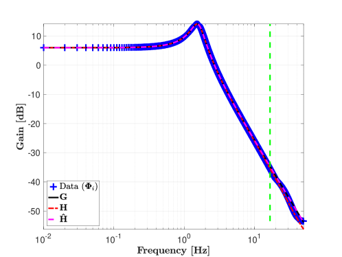
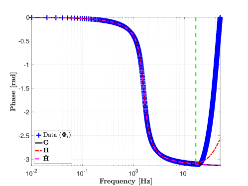
When applied on the chirp signal case presented above, the above discrete frequency response estimation $\mathbf{\Phi}_{i}=\mathbf{y}(\imath\omega_{i})/\mathbf{u}(\imath\omega_{i})\in\mathds{C}^{n_{y}\times n_{u}}$ (denoted H), estimated at samples $\imath\omega_{i}=\imath 2\pi f_{i}$ (W), where $i=1,\dots,N$, is obtained and leads to Figure 5. Interestingly, when comparing the the original linear system $\mathbf{G}$, the overall dynamic seems well cached, even if some errors appear in high frequencies (close to the Nyquist frequency). This observation is consistent with the fact that the chirp function is exciting enough. Note that the frequency plot stops at the Nyquist frequency $f_{\text{Nyquist}}=f_{s}/2=50$Hz, where $f_{s}=100$Hz. Due to the sampling effect, above this Nyquist, the spectrum repeats with this frequency periodicity.

Figure 5: Frequency response gain (top) and phase (bottom) of $\mathbf{G}$ (G) and its discrete estimation $\{\omega_{i},\mathbf{\Phi}_{i}\}$ ({W,H}) using the chirp excitation signal.

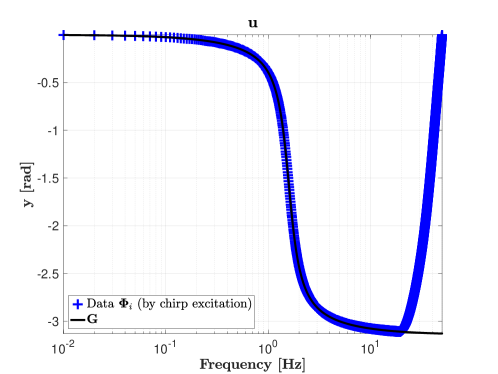
By analysing the frequency response of $\mathbf{G}$ and its estimated discrete samples $\mathbf{\Phi}_{i}$, some differences are observed, even with no noise considered in the measurements. Signal processing theory can bring answers to this discrepancies by considering the effect of sampling and reducing it by using more elaborate techniques. However, at this point, the transfer estimation seems acceptable. Note that in practice, an exact model appears to be a unicorn as model validity can only be considered through the lens of (experimental) data which are affected by many uncertainties. A model should be considered mainly w.r.t. what it will be used for. In our case, the model will mostly serve at designing a controller, and variability should always be considered. This remark is also linked with what people call robustness with respect to some model variability. This specific point is not directly addressed here but interested reader may find clues and more detailed theorems in the very complete book [11].

3 Reduced model construction

As rooted on the input-output collected data from the exciting signal followed by the Fourier transform and cross correlation transfer estimation, one now has access to the $\{\imath\omega_{i},\mathbf{\Phi}_{i}\}_{i=1}^{N}$ couple, denoted {W,H}. From this basis, we are now ready to perform the model construction step. Many techniques are tailored to this objective, but here, let us invoke the interpolatory framework to construct a rational model $\mathbf{H}$ as well as its approximation $\mathbf{\hat{H}}$ (see [2] for complete description and presentation of "interpolatory" problem and meaning).

3.1 Data-driven approximation

Given the complex-valued input-output data collection $\{z_{i},\mathbf{\Phi}_{i}\}_{i=1}^{N}$ or more specifically in our case $\{\imath\omega_{i},\mathbf{\Phi}_{i}\}_{i=1}^{N}$ (where $z_{i}\in\mathds{C}$, $\omega_{i}\in\mathds{R}$ and $\mathbf{\Phi}_{i}\in\mathds{C}^{n_{y}\times n_{u}}$) defined as,

$$\mathbf{y}(z_{i})=\mathbf{\Phi}_{i}\mathbf{u}(z_{i})\text{ or }\mathbf{y}(\imath\omega_{i})=\mathbf{\Phi}_{i}\mathbf{u}(\imath\omega_{i}),$$ (11)

the approximation problem aims at constructing the approximate rational transfer function matrix $\mathbf{\hat{H}}$ mapping inputs $\mathbf{u}$ to the approximate outputs $\mathbf{\hat{y}}$ such that

$$\mathbf{\hat{y}}(s)=\mathbf{\hat{H}}(s)\mathbf{u}(s).$$ (12)

Obviously, some objective are that (i) the reduced inputs to outputs map should be "close" to the original i.e. for the same $\mathbf{u}$, $\mathbf{\hat{y}}$ close to $\mathbf{y}$ in some sense, (ii) the critical system features and structure should be preserved, and, (iii) the strategies for computing the reduced system should be numerically robust and stable. Approximating $\mathbf{G}$ with (12) is a model-based approximation, while, approximating its input-output data $\{\imath\omega_{i},\mathbf{\Phi}_{i}\}_{i=1}^{N}$ with (12) belongs to the data-driven family (see [1, 9] for examples). Here we first follow the data-driven philosophy and secondly the model-based one. In both cases, the interpolation lens of is used.

In the data-driven model approximation, the main ingredient is the Loewner framework initially settled in [7]. Interested reader can also find details in [2] and practical clues and applications in [9]. In brief, the Loewner approach is a data-driven method building a rational descriptor LTI dynamical model $\mathbf{H}$ of dimension $m$ of the same form as (3), which interpolates frequency-domain data given as (11). It is rooted on the so-called Loewner and shifted Loewner matrices which provide information on the minimal order of the interpolating underlying rational function. The MOR toolbox provides an implementation of this method, which can be called as follows

⬇

% Approximation from data

opt = [];

opt.verbose = true;

opt.sample = floor(length(W)/256); % undersampling to fasten approximation

opt.freqBand = [0 Fnyq/3]*2*pi; % frequency band of approximation

opt.ensureStab = true; % enforce model stability

[Hi,info_i] = mor.lti({W,H},[],opt); % [] means that the exact order model is sought

Listing 4: Example file start2ndOrder.m: data-driven model construction.

On the basis of the frequency W (i.e. $\imath\omega_{i}$) and corresponding frequency responses H (i.e. $\mathbf{\Phi}_{i}$) set, the above code computes Hi (i.e. $\mathbf{H}$), a minimal order interpolating rational function equipped with a descriptor state-space realisation. With the arguments provided in the mor.lti routine, the approximation is done up to the frequency $f_{\text{Nyquist}}/3$ (indeed when analysing the data obtained during the transfer function estimation, strange behaviour is observed after this frequency and are thus discarded in this step), data are under-sampled (for numerical simplicity) and the output Hi model is forced to be input-output stable. The following information are also listed.

⬇

| Selected order : 58 |

| RHinf sigma/gamma : 0.3587/0.3587 (optimal) |

+——————————————————————————+

Listing 5: Example file start2ndOrder.m: generate and simulate a chirp signal excitation.

Briefly, the above information set displayed after executing this MOR toolbox code mainly indicates that an order $n=58$ of function $\mathbf{H}$ (Hi) has been obtained. This order is automatically computed by the procedure. At this point, a model $\mathbf{H}$ of dimension $n=58$ is then obtained. Of course, considering the original system $\mathbf{G}$ (of oder 2), such an order is way too large, but considering the interpolatory objective this not specifically strange. We won’t enter into details here and will focus our attention on its frequency response, later presented on Figure 5, showing that it really well capture the data collected, and restitute the behaviour of $\mathbf{G}$ (obviously with a way too large function). As this function is of high order, in view of control design, it is well admitted that a reduction step is necessary. Indeed, most of the control methods are very limited to model with low order models and numerical accuracy is expected with simpler models.

3.2 Model reduction

As rooted on the obtained interpolated model $\mathbf{H}$ (Hi), a $n_{u}$ inputs, $n_{y}$ outputs linear dynamical system described by the complex-valued function from $\mathbf{u}$ to $\mathbf{y}$, of order $n$ ($n$ large or $\infty$)

$$\mathbf{H}:\mathds{C}\rightarrow\mathds{C}^{n_{y}\times n_{u}},$$

the model approximation problem consists in finding $\mathbf{\hat{H}}$ of order $r\ll n$

$$\mathbf{\hat{H}}:\mathds{C}\rightarrow\mathds{C}^{n_{y}\times n_{u}},$$

that well reproduces the input-output behaviour and equipped with realisation

$$\mathbf{\hat{H}}(s)={\hat{C}}(s{\hat{E}}-{\hat{A}})^{-1}{\hat{B}},$$

where ${\hat{E}},{\hat{A}}\in\mathbb{R}^{r\times r}$, ${\hat{B}}\in\mathbb{R}^{r\times n_{u}}$ and ${\hat{C}}\in\mathbb{R}^{n_{y}\times nr}$, are constant matrices. One standard way to deal with this problem is to consider the ${\mathcal{H}_{2}}$ model approximation problem given as follows.

$$\mathbf{\hat{H}}:=\arg\min_{\small\begin{array}[]{c}\mathbf{G}\in{\mathcal{H}_{2}}\\ \mathbf{rank}(\mathbf{G})=r\ll n\end{array}\normalsize}||\mathbf{H}-\mathbf{G}||_{{\mathcal{H}_{2}}}$$

Such a problem can be solved using the MOR toolbox through the mor.lti interface, as detailed in the following code, where one aims at finding an optimal model $\mathbf{\hat{H}}$ (Hr) of dimension $r=2$, on the basis of $\mathbf{H}$ (Hi). Here the order two has been selected for illustration purpose, but as $\mathbf{H}$ (Hi) is of dimension $n=58$, different choice may also have been done. Still, as the considered example $\mathbf{G}$ is a second order, let us continue with this assumption.

⬇

% Model order reduction

[Hr,info_r] = mor.lti(Hi,2,opt);

Listing 6: Example file start2ndOrder.m: model reduction step.

Applied on the obtained $\mathbf{H}$ (Hi) model, the above code leads to the following output, illustrating among other, the iterative aspect of the approach.

⬇

| 3 0 0.14 |

+——————————————————————————+

Listing 7: Example file start2ndOrder.m: generate and simulate a chirp signal excitation.

After convergence, the obtained models $\mathbf{H}$ (Hi) and $\mathbf{\hat{H}}$ (Hr) Bode responses are shown on Figure 5. Clearly, it illustrates that the model $\mathbf{G}$ is well captured by $\mathbf{H}$ of dimension 58, but also by $\mathbf{\hat{H}}$ of order 2, being the same order as the original $\mathbf{G}$.

Figure 6: Frequency response gain (top) and phase (bottom) of the original data (blue $\mathbf{+}$), original model $\mathbf{G}$ (solid black), full order interpolated model $\mathbf{H}$ (Hi dashed red) and reduced order model $\mathbf{\hat{H}}$ (Hr dashed pink).

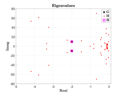
One interesting complement concerns the pencil associated to the dynamical matrices couple for all models, $\mathbf{G}$, $\mathbf{H}$ and $\mathbf{\hat{H}}$. While the interpolating full order model $\mathbf{H}$ exhibits 58 singularities, both the $\mathbf{G}$ ad $\mathbf{\hat{H}}$ have only two of them. Even more interestingly, these two last models have the exact same eigenvalues, as shown on Figure 7, meaning that on the sole basis of system $\mathbf{\Sigma}$ excitation plus model interpolation and approximation, one is able to recover the original model dynamical information without knowing it a priori. This last statement is a very strong one and is obviously valid in linear dynamical systems theory only. It is one of the real strength of model approximation in the linear domain.

Figure 7: Eigenvalues of the original model $\mathbf{G}(s)$ (black $\mathbf{\times}$), full order interpolated model $\mathbf{H}$ (red $\mathbf{\cdot}$) and reduced order model $\mathbf{\hat{H}}$ (pink square).

4 Control design (${\mathcal{H}_{\infty}}$-norm oriented)

On the basis of the simplified model obtained $\mathbf{\hat{H}}$ (Hr), being as accurate as possible but also as simple as possible, we are now ready to design a controller to achieve some closed-loop performances. Here, our simple objective is to make our output $\mathbf{y}$ track an exogenous reference signal denoted $\mathbf{r}$. Such an objective is a fairly standard one and our aim is more to illustrate in practice how this can be easily done using existing numerical tools. Indeed, authors believe that extension of this problem to more complex cases can be "easily" done once this one well mastered.

4.1 Preliminary words

The control design for linear systems is a wide problem on which many researchers and practitioners have proposed methodological results and numerical schemes to achieve different objectives. In this report we only focus on the so called ${\mathcal{H}_{\infty}}$ control approach, well known in the robust control community for its fantastic robustness and performance definition versatility (see e.g. [4, 11] for a very good starting point). Here we follow the ${\mathcal{H}_{\infty}}$ philosophy which objective is, on the basis of the simplified model $\mathbf{\hat{H}}$, to design a controller $\mathbf{K}$ such that,

$$\mathbf{K}:=\arg\min_{\small\begin{array}[]{c}\mathbf{\tilde{K}}\in{\mathcal{H}_{\infty}}\\ \mathbf{\tilde{K}}\in\mathcal{K}\end{array}\normalsize}||\mathcal{F}_{l}(\mathbf{\hat{H}},\mathbf{\tilde{K}})||_{{\mathcal{H}_{\infty}}}$$ (13)

where $\mathcal{F}_{l}(\cdot,\cdot)$ is the lower fractional operator (see [11, 6] for a good insight), $\mathcal{K}$ is the class of controller considered (we will come back to this later in this section) and ${\mathcal{H}_{\infty}}$ denotes either the space of complex-valued functions with bounded supremum over the imaginary axis or the norm associated. More specifically, $\mathbf{T}_{\mathbf{r}\mathbf{y}}(\mathbf{\hat{H}})=\left.\mathcal{F}_{l}(\mathbf{\hat{H}},\mathbf{\tilde{K}})\right\rvert_{\mathbf{\tilde{K}}=\mathbf{K}}$ is nothing but the closed-loop illustrated on Figure 8, when the controller is defined as

$$\mathbf{u}(s)=\mathbf{K}(s)\mathbf{e}(s)=\mathbf{K}(s)(\mathbf{r}(s)-\mathbf{y}(s)),$$

where $\mathbf{e}$ is the error signal and $\mathbf{r}$, the reference one.

Figure 8: Closed-loop scheme of $\mathbf{T}_{\mathbf{r}\mathbf{y}}(\mathbf{\hat{H}},\mathbf{K})$, being the interconnection of $\mathbf{K}$ with model $\mathbf{\hat{H}}$, involved in the synthesis step.

Remembering that for SISO systems the ${\mathcal{H}_{\infty}}$ norm is the peak value of the Bode gain response, as it problem (13) is not really interesting to solve. Indeed minimising the gain of the interconnection shown in Figure 8 is not specifically relevant. This why instead of solving (13), one aims at solving a modified version of it, through what is generally called, the generalised problem, involving the generalised plant. Such a notion is more detailed in the sequel.

4.2 The ${\mathcal{H}_{\infty}}$-norm oriented control design

One essential ingredient in linear control, and so it is in ${\mathcal{H}_{\infty}}$ control, is the generalised plant concept. Basically, it consists in constructing a plant including the model $\mathbf{\hat{H}}$ and a set of performance output $\mathbf{W}_{o}$ and input $\mathbf{W}_{i}$ weighting functions. These weighing functions are interconnected to the plant’s model and constitute the basis of the control optimisation process. Practically, they shape the interconnection to be minimised where performances and control objectives are encapsulated in these weighting functions (again, reader may refer to [11]). Before illustrating such a generalised plant and how it is constructed, let us just recast the original ${\mathcal{H}_{\infty}}$ control problem (13) now as

$$\mathbf{K}:=\arg\min_{\small\begin{array}[]{c}\mathbf{\tilde{K}}\in{\mathcal{H}_{\infty}}\\ \mathbf{\tilde{K}}\in\mathcal{K}\end{array}\normalsize}||\overbrace{\mathbf{W}_{o}\mathcal{F}_{l}(\mathbf{\hat{H}},\mathbf{\tilde{K}})\mathbf{W}_{i}}^{\mathbf{T}(\mathbf{\hat{H}},\mathbf{\tilde{K}})=\mathcal{F}_{l}(\mathbf{P},\mathbf{\tilde{K}})}||_{{\mathcal{H}_{\infty}}}$$ (14)

where $\mathbf{W}_{o}$ and $\mathbf{W}_{i}$ are designer parameters shaping the closed-loop transfer. At this point it is important to note that the selection of $\mathbf{W}_{o}$ and $\mathbf{W}_{i}$ can be viewed as an "art" since they completely affect the result in an indirect way. Indeed, engineers are often required to modify the weights and re-optimise, observe the result, and keeping iterating until the expected solution is reached. Still, as we will see in the considered example, some intuitions can be felt when practicing a bit. In the following code, and keeping in mind the tracking objective we construct such a generalised plant $\mathbf{T}(\mathbf{\hat{H}},\mathbf{\tilde{K}})=\mathcal{F}_{l}(\mathbf{P},\mathbf{\tilde{K}})$. This is done by first defining the $\mathbf{P}$ (P) operator as follows.

⬇

% Construction of the generalised plant embedding the performances

alpha = 1e3;

wc = 1;

Wu = tf([1/wc 1],[1/(wc*alpha) 1]); % weight the control signal

We = 10/tf([1 0],[1/1e0 1]); % weight the tracking error signal

systemnames = ’Hr We Wu’; % declare the dynamical systems

inputvar = ’[r; u]’; % declare the input signals sorted as [w u]

outputvar = ’[Wu; We; r-Hr]’; % declare the output signals sorted as [z y]

input_to_Hr = ’[u]’; % input of the system Hr

input_to_Wu = ’[u]’; % input of the control weigh Wu

input_to_We = ’[r-Hr]’; % input of the tracking error weight We

cleanupsysic = ’yes’; % remove from workspace sysic variables

P = sysic; % create the sysetm interconnection

./code/start.m

Listing 8: Example file start2ndOrder.m: $\mathbf{P}$ (P) matrix transfer construction.

Following the above code, we define and interconnect two functions $\mathbf{W}_{u}$ (Wu) and $\mathbf{W}_{e}$ (We) as weights on the control signal $\mathbf{u}$ and error signal $\mathbf{e}$ respectively. These weights lead to the new fictive outputs $\mathbf{z}_{u}$ and $\mathbf{z}_{e}$ and the resulting generalised model $\mathbf{P}$ now embeds the following input-output transfers

$$\left[\begin{array}[]{c}\mathbf{z}_{u}\\ \mathbf{z}_{e}\\ \mathbf{r}-\mathbf{y}\end{array}\right]=\left[\begin{array}[]{cc}0&\mathbf{W}_{u}\\ \mathbf{W}_{e}&-\mathbf{W}_{e}\mathbf{\hat{H}}\\ 1&-\mathbf{\hat{H}}\end{array}\right]\left[\begin{array}[]{c}\mathbf{r}\\ \mathbf{u}\end{array}\right]=\mathbf{P}\left[\begin{array}[]{c}\mathbf{r}\\ \mathbf{u}\end{array}\right],$$ (15)

where $\mathbf{P}\in\mathds{C}^{3\times 2}$ is a complex-valued matrix function completely defined by the model $\mathbf{\hat{H}}$ and the weights defined as

$$\mathbf{W}_{u}=\frac{s+1}{s/1000+1}\text{ and }\mathbf{W}_{e}=10\frac{s+1}{s},$$

being a high pass filter with cut-off frequency at $2\pi$Hz and an integral-like with cut-off also at $2\pi$Hz, respectively (we will come back later on the reason for using such performances). With reference to (15), reader may note that the first two outputs are the performances on the control signal tracking error respectively and that the last output is the measurement. Similarly, the first input is the reference while the second one is the control signal. A more systematic way to represent $\mathbf{P}$ is then given as

$$\left[\begin{array}[]{c}\mathbf{z}\\ \mathbf{e}\end{array}\right]=\mathbf{P}\left[\begin{array}[]{c}\mathbf{w}\\ \mathbf{u}\end{array}\right],$$

where $\mathbf{z}$ is the performance output vector gathering the variables to control, or more specifically to minimise (here $\mathbf{z}_{u}$ and $\mathbf{z}_{e}$) and $\mathbf{w}$ the exogenous signals vector gathering references, disturbances (here only the reference $\mathbf{r}$). Now $\mathbf{P}$ has been described, let us define Ktilde, the controller $\mathbf{\tilde{K}}$ structure we want to optimise. Here, without entering into technical considerations, we chose a SISO (we measure $\mathbf{e}=\mathbf{r}-\mathbf{y}$ and control $\mathbf{u}$) controller of dimension $n_{c}=2$. In addition we select a controller with no direct feedthrough, e.g. a full ${E}$ matrix. The following Matlab code stands.

⬇

% Controller structure definition

ncon = 1; % number of control variables

nmeas = 1; % number of measured variables

nc = 2; % number of internal variables

Ktile = ltiblock.ss(’Ktilde’,nc,ncon,nmeas);

Ktile.d.Free = zeros(ncon,nmeas);

Ktile.d.Value = zeros(ncon,nmeas);

./code/start.m

Listing 9: Example file start2ndOrder.m: definition of the controller $\mathbf{\tilde{K}}$ (Ktilde) structure. This script defines in some sense the $\mathcal{K}$ function space, giving the admissible $\mathbf{\tilde{K}}$ set.

Previously, in (14), the space $\mathcal{K}$ of admissible controllers was introduced. Such a space is somehow defined with the above code by considering the space of SISO controllers of dimension two with no direct feed-through. More specifically, one seeks a controller $\mathbf{K}$ embedding a state-space model as

$$\left(\left[\begin{array}[]{cc}1&0\\ 0&1\end{array}\right],\left[\begin{array}[]{cc}a_{1}&a_{2}\\ a_{3}&a_{4}\end{array}\right],\left[\begin{array}[]{c}b_{1}\\ b_{2}\end{array}\right],\left[\begin{array}[]{cc}c_{1}&c_{2}\end{array}\right],0\right),$$

where all coefficients $a_{i}$, $b_{i}$ and $c_{i}$ are real and considered as design variables. Up to now, one has $\mathbf{P}$, being a known transfer matrix solely defined by the model $\mathbf{\hat{H}}$ and the weighting functions ($\mathbf{W}_{i}=1$ and $\mathbf{W}_{i}=\textbf{blkdiag}(\mathbf{W}_{u},\mathbf{W}_{e})$), and $\mathbf{\tilde{K}}$, a structured controller with gains to be optimised. Then we have all the ingredients to set up our (once again modified) ${\mathcal{H}_{\infty}}$ control problem as follows.

⬇

% Model-based Hinf-controller oprimisation (hinfstruct)

T = lft(P,Ktile); % lower LFT

Wk = 1e-9*tf(1,1); % almost unconstrained gain

Text = append(T,Wk*Ktile); % enforce ’K’ stability

option = hinfstructOptions(’Display’,’iter’, …

’RandomStart’,0, …

’MaxIter’,500);

[CLopt,gamma,info] = hinfstruct(Text,option);

K = ss(CLopt.Blocks.Ktilde);

./code/start.m

Listing 10: Example file start2ndOrder.m: construction of the extended generalised plant $\mathbf{T}$ (both T and Text) and optimal values of $\mathbf{K}$ (K).

More in details, the above code now considers an extended version of the ${\mathcal{H}_{\infty}}$ problem, slightly different to (14), formulated as follows.

$$\mathbf{K}:=\arg\min_{\small\begin{array}[]{c}\mathbf{\tilde{K}}\in{\mathcal{H}_{\infty}}\\ \mathbf{\tilde{K}}\in\mathcal{K}\end{array}\normalsize}\begin{array}[]{c}||\mathbf{T}(\mathbf{\hat{H}},\mathbf{\tilde{K}})||_{{\mathcal{H}_{\infty}}}\\ ||\mathbf{\tilde{K}}\mathbf{W}_{k}||_{{\mathcal{H}_{\infty}}}\end{array}$$ (16)

where $\mathbf{W}_{k}$ is an additional weighting function (here a simple gain) applied directly on the controller $\tilde{\mathbf{K}}$ to enforce the transfer $\tilde{\mathbf{K}}\mathbf{W}_{k}$ to be stable. In the case described by (16), the two performance channels ${\mathbf{T}(\mathbf{\hat{H}},\mathbf{\tilde{K}})}$ and ${\mathbf{\tilde{K}}\mathbf{W}_{k}}$ are appended, leading to the Text variable, gathering the two objectives. Problem (16) is (NP-)hard to solve (so was also (14)) and has been the subject of many research contributions. However, thanks to the developments of the hinfstrut routine embedded in the Matlab software based on the seminal contribution [3], a numerically robust solution can be obtained in a resonable time. The above code first computes the extended generalised variable Text and then calls the hinfstruct routine to obtain K, the optimal controller $\mathbf{K}$, solving problem (16).

Then, such code leads to the following informations (note that values may differ from a version and computer to an other).

⬇

than physical instabilities.

Listing 11: Example file start2ndOrder.m: construction of the extended generalised plant $\mathbf{T}$ (both T and Text) and optimal values of $\mathbf{K}$ (K).

The last warning is not an issue in our case. Indeed, it states that some instabilities cannot be controlled. In our case, this is caused by the $\mathbf{W}_{e}$ weight function exhibiting an integral action and thus $\mathbf{P}$ has an eigenvalue in zero being uncontrollable.

Figure 9: Closed-loop scheme of $\mathbf{T}_{\mathbf{r}\mathbf{y}}(\mathbf{G},\mathbf{K})$, being the interconnection of $\mathbf{K}$ with model $\mathbf{G}$, involved in the validation step.

Now that an optimal controller $\mathbf{K}$ (denoted K) has been obtained, we can analyse the resulting closed-loop. More specifically, the following code constructs the closed-loop as shown on Figure 9, involving the original model $\mathbf{G}$. The associated Bode gain and step responses are shown on Figures 10 and 11.

⬇

% Closed-loop created with G instead of Hr, looped with K (continuous-time)

systemnames = ’G K’;

inputvar = ’[r]’;

outputvar = ’[G; r-G; K]’;

input_to_G = ’[K]’;

input_to_K = ’[r-G]’;

cleanupsysic = ’yes’;

CL = sysic;

CL = balreal(CL);

./code/start.m

Listing 12: Example file start2ndOrder.m: construction of te closed-loop model when original system $\mathbf{G}$ looped with $\mathbf{K}$.

Figure 10: Bode gain of the original model $\mathbf{G}$ (blue) and closed-loop $\mathbf{T}_{\mathbf{r}\mathbf{y}}(\mathbf{G},\mathbf{K})$ (red). Note the static gain and peak damping.

Figure 11: Step response of the original model $\mathbf{G}$ (blue) and closed-loop $\mathbf{T}_{\mathbf{r}\mathbf{y}}(\mathbf{G},\mathbf{K})$ (red). Note the static gain and peak damping.

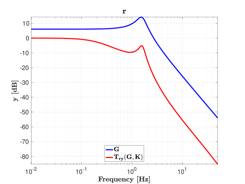
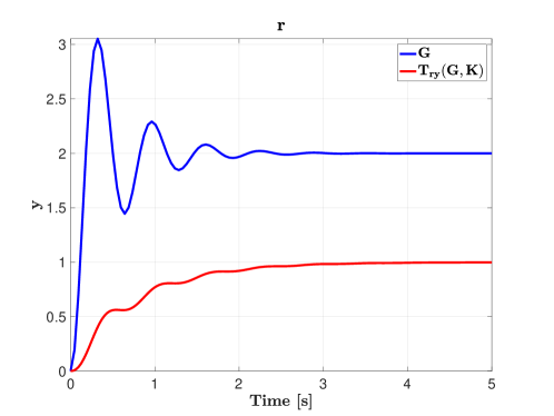
One observes on Figure 10 that the bump present on te open-loop original $\mathbf{G}$ model has been attenuated (i.e. damped) and the static gain is now at 0dB, meaning that the output $\mathbf{y}$ should track $\mathbf{r}$ in steady-state. In addition, Figure 11 assesses these observations, showing the step response of $\mathbf{G}$ and $\mathbf{T_{ry}}$ obtained using $\mathbf{G}$ looped with $\mathbf{K}$. One important validation when applying ${\mathcal{H}_{\infty}}$ control design is the validation of the weighting constraints. This is done on Figures 12 and 13, where the transfer $\mathbf{T_{re}}$ and $\mathbf{T_{ru}}$ are plotted, and compared to the weighting functions $\gamma/\mathbf{W}_{e}$ and $\gamma/\mathbf{W}_{u}$ respectively (where $\gamma$ denotes the ${\mathcal{H}_{\infty}}$ norm obtained when solving (16)).

Figure 12: Bode gain of the weighting function on the tracking performance $\gamma/\mathbf{W}_{e}$ (black dashed) and closed-loop $\mathbf{T_{rz_{e}}}(\mathbf{G},\mathbf{K})$ (red).

Figure 13: Bode gain of the weighting function on the control performance $\gamma/\mathbf{W}_{u}$ (black dashed) and closed-loop $\mathbf{T_{rz_{u}}}(\mathbf{G},\mathbf{K})$ (red).

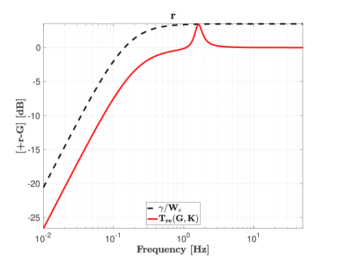
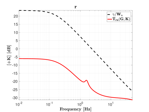
First, one should note that both transfers are upper bounded by the corresponding weighting functions (black dash dotted), assessing that the considered frequency templates $\mathbf{T(\mathbf{\hat{H}},K)}$ (indeed $\mathbf{T(\mathbf{G},K)}$) are satisfied, i.e. $||\mathbf{T(\mathbf{G},K)}||_{{\mathcal{H}_{\infty}}}\leq\gamma/\mathbf{W}_{x}$ where $x=\{u,e\}$. The second objective being $||\mathbf{K}||_{{\mathcal{H}_{\infty}}}\leq\gamma\mathbf{W}_{k}$ is also (largely since $W_{k}=10^{-9}$) satisfied. Remember that such a objective was used only to ensure that the obtained controller $\mathbf{K}\in{\mathcal{H}_{\infty}}$, i.e. is stable.

At this point, let us just make a quick remark on the section of $\mathbf{W}_{u}$ and $\mathbf{W}_{e}$. The first one affects the control signal $\mathbf{u}$ and is thus selected so that $1/\mathbf{W}_{u}$ rolls-off in high frequencies to avoid noise amplification. Similarly, the $\mathbf{W}_{e}$ function, acting on the error signal $\mathbf{r}-\mathbf{y}$, is standardly selected so that in low frequency $1/\mathbf{W}_{e}$ has a low (zero) gain to ensure no steady-state error up to a certain cut-off frequency (being the time response) and constant gain at infinity to monitor the margin performances (as shown in the next part).

4.3 A glimpse of margin

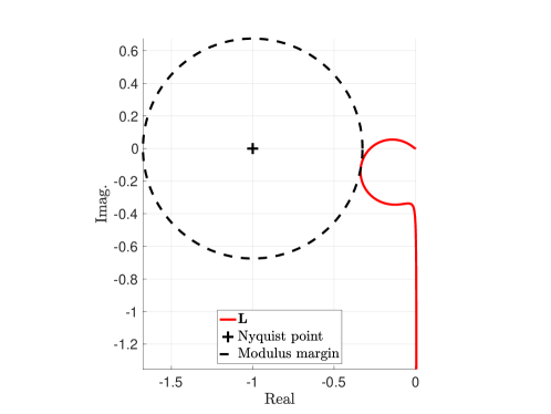
Entering in a complete margin analysis is not the objective of this simple report (interested reader should refer e.g. to [11, 6]). Still, to give a grasp of the concept, margins are generally computed on the following transfer (availability and/or complexity usually make the decision),

$$\mathbf{L}(s)=\mathbf{G}(s)\mathbf{K}(s)\text{ or }\mathbf{L}(s)=\mathbf{H}(s)\mathbf{K}(s)\text{ or }\mathbf{L}(s)=\mathbf{\hat{H}}(s)\mathbf{K}(s)$$

which represents the loop interconnection without closing the loop. This transfer is actually very important to monitor in practice. Actually, a whole class of design method, called loop-shaping, are rooted on this transfer and aim at shaping it through adequate filtering. Among interesting margin, the modulus margin, denoted ModMargin, is defined as

$$\textbf{MM}=\dfrac{1}{||1-\mathbf{T_{ry}}||_{{\mathcal{H}_{\infty}}}},$$

is a unifying quantity of the gain and phase margins and represents the maximal gain of the so-called sensitivity function, being the transfer from the reference to the error (and thus connected to the weighting function $\mathbf{W}_{e}$). These last components can be obtained through the allmargin routine embedded in Matlab and recalled hereafter.

⬇

% A glimpse of margin (continuous-time)

L = G*K;

[reNyq,imNyq] = nyquist(L);

allmargin(L)

ModMargin = 1/norm(CL(2,1),inf);

Listing 13: Example file start2ndOrder.m: some margins.

Note that complete books are dedicated to the robustness, margin, and related points in the control literature. It is quite hard sorting them, but reader should keep in mind that many numerical tools are embedded in the Matlab software, providing a good starting point.

⬇

Stable: 1

Listing 14: Example file start2ndOrder.m: construction of te closed-loop model when original system $\mathbf{G}$ looped with $\mathbf{K}$.

Figure 14 also shows the Nyquist plot of $\mathbf{L}$, as well as the Nyquist point and the modulus margin illustration. Usually, a modulus margin of $0.5$ is considered as a very good one (note that optimal LQ control for SISO systems ensures this modulus margin).

Figure 14: Nyquist plot of the loop transfer $\mathbf{L}$ (solid red), Nyquist stability point (black $+$) and modulus margin (black dashed circle).

4.4 Discrete-time controller and hybrid loop

Now the optimal continuous-time controller $\mathbf{K}$ (K) has been obtained, in view of implementation purpose, it is needed to discretise it to obtain a sampled-system. This step is subject to many research as well and one may refer to [10] for some insight. Without being too specific, the standard bilinear Mobius transform (also celebrated as Tustin stransformation) is used. It basically consists in a transformation from the $s$-plane to the $z$-plane using the following formulae

$$s=\dfrac{2}{T_{s}}\dfrac{z-1}{z+1},$$

where $T_{e}$ is the sampling time. In Matlab this transformation is implemented and can be obtained as follows.

⬇

% Controller continuous vs. sampled (discretisation using Matlab)

Ts = 1e-2; % sampling time of the controller

K_z = c2d(K,Ts,’tustin’); % bilinear discretisation method

FR_K_z = freqresp(K_z,W);

./code/start.m

Listing 15: Example file start2ndOrder.m: discretisation step using bilinear transformation.

Figure 15: Comparison of the controller Bode response. $\mathbf{K}$ (K) in continuous-time (solid blue) and $\mathbf{K}_{z}$ (K_z) in sampled-time at $T_{s}=10$ms (red dashed).

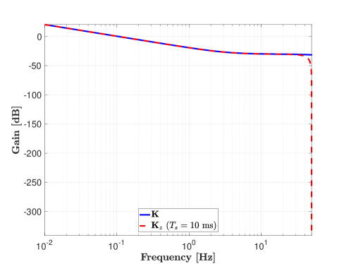
The above code then creates the discrete-time controller $\mathbf{K}_{z}$ (denoted K_z) obtained with a sampling time $T_{s}=10$ms defined as follows, and for which frequency response (Bode diagram) is given in Figure 15.

⬇

Discrete-time state-space model.

Listing 16: Example file start2ndOrder.m: discretisation step using bilinear transformation.

When analysing Figure 15, one first note that the continuous-time response of $\mathbf{K}$ is similar to the $\mathbf{K}_{z}$ up to $f_{\text{Nyquist}}=f_{s}/2=1/(2T_{s})=5$Hz. Moreover, as the bilinear transformation maps the vertical axis $\imath\mathds{R}$ onto the unit circle, the spectrum is naturally repeated every $f_{\text{Nyquist}}$, resulting in these sharp peaks in the Bode gain responses at this frequency (and its periodic multiplicities).

Figure 16: Comparison of the controller Bode response. $\mathbf{K}$ in continuous-time (solid blue) and $\mathbf{K}_{z}$ in sampled-time (red dashed). From top left to bottom right $T_{s}=50$, $T_{s}=100$, $T_{s}=200$ and $T_{s}=500$ms.

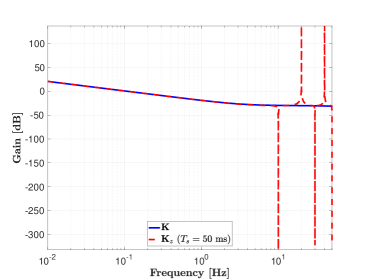
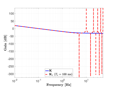
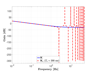
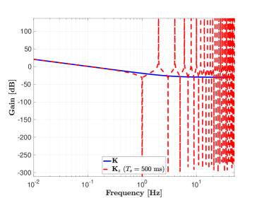
Obviously, one can reduce the sampling time as much as possible, leading to a better frequency response matching, but with a technical and practical limitation (and cost). A glimpse of the impact of the sampling frequency is shown on Figure 16 which highlights the effect of decreasing the sampling frequency. It is clear the slower the discretisation, the less the discrete controller $\mathbf{K}_{z}$ matches the (reference) continuous one $\mathbf{K}$. In addition, the phase plot is also affected, leading to shift and delay in the loop. This point is not reported here, but it may lead to instabilities (as illustrated in the next section). Many more remarks are available in [10] and references therein.

Figure 17: Closed-loop scheme of $\mathbf{T}_{\mathbf{r}\mathbf{y}}(\mathbf{G},\mathbf{K}_{z})$, being the interconnection of the sampled $\mathbf{K}_{z}$ with model $\mathbf{G}$, involved in the validation step.

One very complex and interesting question arising at this point is to analyse the impact of such discretisation in the closed-loop performances. With reference to Figure 17, the interconnection of the continuous-time model $\mathbf{G}$ with the sampled-time controller $\mathbf{K}_{z}$ is an hybrid system blending continuous and discrete variables. The analysis of such an interconnection is much more involved than the study of a purely continuous-time interconnection and dedicated methods, that go way over the scope of this report, are required.

In the following section, this sampled controller will be interconnected to a modulation box and analysis will be done on this (even more) complex loop. A sketch of solution and the main ideas will be discussed. Theoretical considerations are purposely left aside.

5 Signal modulation and hybrid closed-loop validation

The points evoked in the previous sections are related to dynamical systems theory with the main objective of constructing a digital sampled control law $\mathbf{K}_{z}$ achieving some performances. From now, we consider that such a controller has to be implemented with an additional limitation on the actuator capability. More specifically, here we consider the interconnection of a sampled-time controller with a continuous-time system and the effect of a pulsed width modulation in the actuator.

5.1 Preliminary words

Let us now consider that an actuator, between the system and the controller is no longer able to deliver a continuously value $\mathbf{u}(t)$, or more specifically $\mathbf{u}(t_{k})$ (at each sample $T_{s}$), but a pulsed value with varying duration only, being either $\mathbf{u}_{\textbf{min}}$ or $\mathbf{u}_{\textbf{max}}$. This case is illustrated on Figure 18, where the PWM (Pulsed Width Modulation) block is detailed in what follows. Note that in this section, no Matlab code is provided as this part is still under high investigation from the authors, and description of the code would be quite complicated for this tutorial.

Figure 18: Closed-loop scheme of $\mathbf{T}_{\mathbf{r}\mathbf{y}}(\mathbf{G},\mathbf{K}_{z}+\textbf{PWM})$, being the interconnection of the sampled $\mathbf{K}_{z}$ with model $\mathbf{G}$, where control is modulated by the PWM.

5.2 The pulsed width modulation case

The PWM block uses a rectangular impulsion signal taking values between $\mathbf{u}_{\text{min}}$ and $\mathbf{u}_{\text{max}}$ and which length is modulated. This modulation results in variation of the mean $\overline{\mathbf{u}^{\star}}(t_{k})$ of the signal $\mathbf{u}^{\star}(t_{k})$ to convert. If one considers an impulsion with a high frequency $f_{c}$ and a duty cycle $D\in[0~{}1]$, the mean value of the resulting signal is given by

$$\begin{array}[]{rcl}\overline{\mathbf{u}^{\star}}(t_{k})&=&\dfrac{1}{T_{c}}\displaystyle\int_{0}^{T_{c}}\mathbf{u}^{\star}(t_{k})dt_{k}\\ &=&\dfrac{1}{T_{c}}\bigg{(}\displaystyle\int_{0}^{DT_{c}}\mathbf{u}_{\text{max}}dt_{k}+\displaystyle\int_{DT_{c}}^{T_{c}}\mathbf{u}_{\text{min}}dt_{k}\bigg{)}\\ &=&D\mathbf{u}_{\text{max}}+(1-D)\mathbf{u}_{\text{min}}\\ &=&D\mathbf{u}_{\text{max}}\text{ (for $\mathbf{u}_{\text{min}}=0$)}.\end{array}$$ (17)

Obviously, the PWM should be $N\in\mathbb{N}$ times higher than the signal $\mathbf{u}^{\star}(t_{k})$ to be modulated. In practical applications, a simple way to generate the PWM is to use the intersection method which simply requires a saw-tooth carrier signal denoted $\mathbf{u}_{c}(t_{k})$, with frequency $f_{c}=f_{s}/N$ and amplitude from $\mathbf{u}_{\text{min}}=\min\mathbf{u}^{\star}(t_{k})$ to $\mathbf{u}_{\text{max}}=\max\mathbf{u}^{\star}(t_{k})$, that should be compared to the incoming signal $\mathbf{u}^{\star}(t_{k})$. When $\mathbf{u}_{c}(t_{k})>\mathbf{u}^{\star}(t_{k})$, then $\mathbf{u}(t_{k/N})=\mathbf{u}_{\text{max}}$, and $\mathbf{u}(t_{k/N})=\mathbf{u}_{\text{min}}$ otherwise. In our case, the carrier signal has the same period as the control $\mathbf{u}^{\star}(t_{k})$ and the modulated signal is $N=10$ times faster.

5.3 Time-domain simulations

On the basis of the above controller $\mathbf{K}_{z}$ connected to a PWM block as the one described in the previous section, following Figure 18, we are now ready to perform different time-domain simulations to illustrate the efficiency and limitations of the such an interconnection. In the following Figures 19 and 20-21, the outputs $\mathbf{y}$ and control signals $\mathbf{u}$, obtained using the different closed-loop schemes and different sampling times ($T_{s}=\{50,100,200,500\}$ms), namely the one on Figure 9, 17 and 18 are presented. In all cases, we use a PWM block that goes $N=10$ times faster. Moreover, the block provides $\mathbf{u}_{\text{min}}=0$ and $\mathbf{u}_{\text{max}}=1$ only. Note at this point that the amplitude of the PWM also plays an important role, but this is clearly out of the linear domain of this report.

Figure 19: From top left to bottom right: $T_{s}=50$ms, $T_{s}=100$, $T_{s}=200$ and $T_{s}=500$ms. Comparison of the controller step responses of the different closed-loop scheme. The continuous-time closed-loop $\mathbf{G}$-$\mathbf{K}$ (solid red), the hybrid continuous-sampled-time $\mathbf{G}$-$\mathbf{K}_{z}$ in (solid blue) and the hybrid continuous-sampled-time and modulated $\mathbf{G}$-$\mathbf{K}_{z}$-PWM (solid magenta).

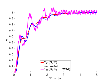
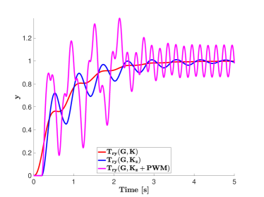
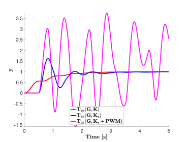
Clearly, when sampling time increases, as shown on Figure 19, the hybrid closed-loop is diverging from the continuous one (tuned in the previous section). This is first observed by comparing the red curve (reference) with the blue one (hybrid loop), where a loss of tracking performance is visible. This observation is even more visible when the control signal is modulated using the PWM block. In the last case ($T_{s}=500$ms), the closed-loop even becomes unstable!

Figure 20: From top left to bottom right: $T_{s}=50$ms, $T_{s}=100$, $T_{s}=200$ and $T_{s}=500$ms. Comparison of the controller control signal of closed-loop scheme. The continuous-time closed-loop $\mathbf{G}$-$\mathbf{K}$ (solid red) and the hybrid continuous-sampled-time $\mathbf{G}$-$\mathbf{K}_{z}$ in (solid blue).

Figure 21: From top left to bottom right: $T_{s}=50$ms, $T_{s}=100$, $T_{s}=200$ and $T_{s}=500$ms. Controller control signal of closed-loop scheme with the hybrid continuous-sampled-time and modulated $\mathbf{G}$-$\mathbf{K}_{z}$-PWM. The blue coloured areas represent the moments where the actuator is high.

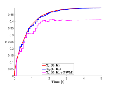
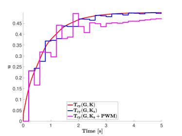
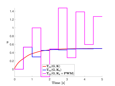
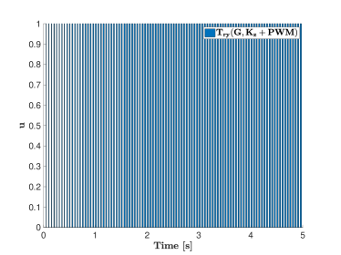
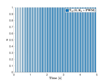
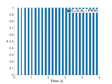
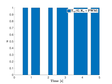
The above observations are completed with Figures 20 and 21 illustrating the control signal sent to the system. On Figure 20 the control signal of the discrete-time controller which sample time is being increased leads to noticeable differences from the reference continuous one. The same comment can be done on Figure 21 which illustrates the pulse sent to the system. These pulses, being larger and larger due to the sampling period increased. Obviously, these observation open the field for more investigation, that will be done in the future.

6 Conclusions

In this report, we aimed at presenting in a condensed and obviously incomplete way, a standard approach for controller design and implementation. We tried to follow what authors believe is a classical control-engineer approach, starting from the system excitation, model identification and reduction, followed by a control design, and ending with some implementation issues related to a pulsed modulation-driven actuator. The report is concentrated on linear problems and nonlinear issues are not really faced here (unless the modulation part). Still, reader should keep in mind that linear dynamical systems and control methods are largely enough for many applications and mastering them is already a nice step forward.

Obviously, the report may be amended, commented and discussed according the reader knowledge, but from the past discussions authors had with multiple users, we feel that such bundle of pages can be a simple but sufficiently good starting point for many practitioners and may be useful for starting discussions.

The objective of the authors was to provide a didactic overview for unfamiliar authors by providing a step by step overview of the general ideas, accompanied with Matlab code involving the MOR Toolbox and some functions available on demand.

References

- [1] A C. Antoulas. Approximation of Large-Scale Dynamical Systems. Advanced Design and Control, SIAM, Philadelphia, 2005.
- [2] A.C. Antoulas, C.A. Beattie, and S. Gugercin. Interpolatory methods for model reduction. SIAM Computational Science and Engineering, Philadelphia, 2020.
- [3] P. Apkarian and D. Noll. Nonsmooth Synthesis. IEEE Transaction on Automatic Control, 51(1):71–86, January 2006.
- [4] B.A. Francis. Lecture Notes in Control and Information, chapter A Course in Control Theory. Heidelberg. Springer-Verlag, February 1987.
- [5] K. Hoffman. Banach spaces of analytic functions. Prentice Hall, 1962.
- [6] J-F. Magni. Linear fractional representation toolbox for use with matlab. Technical report, Onera, Toulouse, France, 2006.
- [7] A J. Mayo and A C. Antoulas. A framework for the solution of the generalized realization problem. Linear Algebra and its Applications, 425(2):634–662, 2007.
- [8] I. Pontes. Large-scale and infinite dimensional dynamical model approximation. Ph.D. thesis, Onera, ISAE, Toulouse University, Toulouse, France, January 2017.
- [9] C. Poussot-Vassal. Large-scale dynamical model approximation and its applications. HDR, habilitation thesis, Onera, INP Toulouse, Toulouse, France, July 2019.
- [10] P. Vuillemin and C. Poussot-Vassal. Discretisation of continuous-time linear dynamical model with the Loewner interpolation framework. submitted (arXiv 1907.10956), 2019.
- [11] K. Zhou and J C. Doyle. Essentials Of Robust Control. Prentice Hall, 1997.