Exact equivalences and phase discrepancies between random matrix ensembles
Abstract.
We study two types of random matrix ensembles that emerge when considering the same probability measure on partitions. One is the Meixner ensemble with a hard wall and the other are two families of unitary matrix models, with weight functions that can be interpreted as characteristic polynomial insertions. We show that the models, while having the same exact evaluation for fixed values of the parameter, may present a different phase structure. We find phase transitions of the second and third order, depending on the model. Other relationships, via direct mapping, between the unitary matrix models and continuous random matrix ensembles on the real line, of Cauchy–Romanovski type, are presented and studied both exactly and asymptotically. The case of orthogonal and symplectic groups is studied as well and related to Wronskians of Chebyshev polynomials, that we evaluate at large .
1. Introduction
Random matrix theory [1] has developed enormously, especially in the last two decades, attracting attention from researchers in a multitude of different fields [2, 3, 4, 5, 6, 7, 8]. Indeed, one of its most exciting aspects is an inherent interdisciplinarity in the study of random matrices. Among the myriad of connections with other mathematical and physical areas, we have the important relationship with the study of random partitions, which in turn is deeply linked with problems in statistical mechanics, as we shall see.
In this work, we will see that random matrix ensembles which are related in different ways, either via direct mapping or emerging as two random matrix descriptions of the same object in the study of random partitions, have the same analytical evaluations for fixed values of the parameters yet, in some cases, the consideration of the large limit leads to a different phase structure.
Originally, we started by noting that the analysis of probabilities given by a finite ensemble with weight of the Meixner type, for example as in [9], could, in principle, equally be studied with a random unitary matrix model, with a distribution of eigenvalues supported on the unit circle. Indeed, we could check, as we shall see, that the corresponding unitary matrix model gives the same results. Furthermore, the equivalence holds for the calculation of correlations near the edge of the eigenvalue density, in a double-scaling limit. However, when studying the more general ensemble with Meixner weight and a hard wall [10] and the corresponding generalized unitary matrix model, while there is again an equivalence for fixed values of the parameter, a different asymptotic behaviour appears, with phase transitions of second order instead of third order. This discrepancy is a consequence of the complexification of the logarithm of the weight function of the more general unitary random matrix ensembles, studied in Section 2.4 below.
We further elaborate on this whole notion by studying other equivalences, with continuous random matrix ensembles on the real line, via direct mapping this time. We first introduce notions of random partitions and how either discrete random matrix ensembles, such as the Meixner ensemble with a hard wall, or continuous unitary random matrix ensembles appear.
Let , , be a partition, and the Schur polynomial associated to it [11], evaluated at . The Schur measure is the probability measure on the space of partitions defined as [12]
| (1.1) |
with normalization constant the inverse of the partition function
where last equality is the Cauchy identity. Here we are denoting the probability taken with respect to a given choice of parameters . Define the set
which encodes the shape of the partition . For a given subset , the probability
that, picking a random partition according to the Schur measure we get , has a determinantal representation. Such representation is the determinant of a known correlation kernel admitting an integral representation [12] (see also [13, Sec. 4]).
In the present work, we are interested in a special case of Schur measure, which is a particular sub-case of what is known in the literature as -measure [14, 15]. For any given the -measure is a probability measure on the partitions of (thus with ) depending on two parameters and . A probability measure over all partitions (with arbitrary) is obtained passing to the grand canonical ensemble, summing over . In defining the grand canonical ensemble, every is weighted with a negative binomial distribution [14].
We choose the parameters in (1.1) to be
| (1.2) |
so that the Schur measure (1.1) becomes a particular instance of -measure with , and the parameter of the binomial distribution being . This choice of is the degenerate case, i.e., non-negative measure, and positive definite when restricted to partitions of length at most . The probabilities
where by we understand the probability taken with specialization of parameters (1.2), admit a determinantal representation in terms of the so-called hypergeometric kernel [14]. The properties of the hypergeometric function were used in [14] to show that, when are integers, the hypergeometric kernel becomes proportional to the Meixner kernel. For a collection of results about the -measure, see the survey [16], and in particular Proposition 6.1 therein for the connection with the Meixner ensemble.
In the present work we are interested in the quantities
| (1.3) |
and (the sum is over all with )
| (1.4) |
with choice of parameter understood to be as in (1.2), and is the size of the partition , corresponding to the total number of boxes in its diagram, and is the dimension of the irreducible representation of the symmetric group labelled by . The meaning of the subscripts and will be clear in a moment. Notice that, due to the property if , the sums are effectively truncated to partitions of length at most . Furthermore, the ratio
is the probability that, picking a random partition with probability distribution as described above, the length of its rows is at most .
The -measure induces a determinantal point process on , thus the correlation functions have determinantal form
for , where is the operator whose kernel, the function on , is the hypergeometric kernel. Therefore we have a Fredholm determinant representation of :
where in the last line is the identity operator. Using the hook-length formula
for the dimension in eq. (1.4) and changing variables , we arrive to the expression
| (1.5) | ||||
where we also used the symmetry in the variables to remove the restriction to the Weyl chamber . is the Barnes -function [17], which, for integer values of the argument is . The expression (1.5) is a Meixner ensemble with summation restricted to and coincides with the partition function of the dimer model studied in [9, 10]111The dimer model is associated with the random tiling of an Aztec diamond with a square [9] or a rectangle [10] cut off. See e.g. the recent work [18] for an overview on dimers, random tilings and random matrices., and has also appeared in [19]. In the Coulomb gas picture, the restriction in the summation range corresponds to a hard wall for the charges (i.e. an infinite barrier) placed at . We assumed , but a completely analogous expression can be easily obtained in the converse case.
Let us introduce the generating functions of, respectively, the complete homogeneous polynomials and the elementary symmetric polynomials , specialized at :
The partition functions (1.3)-(1.4) admit a determinantal representation in terms of determinants of Toeplitz matrices, with symbol, respectively
See for example [20, 21] for the explicit derivation (see also [8] for an extensive account of Toeplitz determinants and their properties). In turn, using Andréief’s identity [22, 23] we have that these Toeplitz determinants admit a representation as unitary matrix integrals
| (1.6) | ||||
| (1.7) |
We will refer to (1.6) and (1.7) as the -model and the -model, respectively. Therefore we have two equivalent matrix model descriptions of the quantity , or, equivalently, of the probability : either as a discrete matrix model on the bounded subset , or as a continuous matrix model on the unit circle.
We stress that the equivalence between these two representations does not rely on a direct map, but rather on a two-step procedure relating the two matrix model formulations of to the same Toeplitz determinant. As a consequence, the quantity , which has the meaning of a deformation parameter, plays different roles in the two pictures. This will be reflected in the mismatch of the phase structure when with .
2. Random matrix ensembles on the unit circle
In the present Section, we consider the asymptotic behaviour of the unitary matrix models defined in eq. (1.6) and (1.7), when the rank is large and scale with . Before that, we comment on the already known aspects of the exact solvability of some of the models above.
2.1. Prologue: Exact evaluation
Following [24], the authors of [10] gave an explicit evaluation of the discrete matrix model (1.5) at the limit value . The exact formula of [10, Proposition 3.1] was obtained thanks to the fact that at the limit value the Meixner ensemble with a hard wall becomes a Hahn ensemble.
On the unitary matrix model side, at (or more generally ) the symbol develops a Fisher-Hartwig singularity, and it can be evaluated exactly thanks to a formula by Böttcher and Silbermann [25] (see also [26] for another proof):
| (2.1) |
This provides an exact check of the equivalence. We will provide a third independent derivation of this result later in Section 3.1.1. For ease of the reader, we report in table 1 the correspondence between the notation of [9, 10], that in [24] and ours.
| In [10] | ||||||
|---|---|---|---|---|---|---|
| In [24] | ||||||
| Here |
Note that, if we choose the symmetric model and modify the symbol by inserting a monomial factor , with , the exact evaluation of the corresponding matrix model at is again given by the formula of [25, 26], thanks to the simple identity
| (2.2) |
when , . The effect of the monomial insertion is to shift the Fourier coefficients of the symbol by : the Fourier coefficient of the symbol is the coefficient of . Therefore, we can evaluate exactly the partition function of the unitary ensemble with weight (2.2), and it is again given by formula (2.1), with .
It is worth mentioning that there are a wealth of analytical results on Toeplitz banded matrices, whose determinant is given by the -models above [27]. More generally, there are many analytical results on determinants of Toeplitz matrices generated by a rational symbol, but we will explore complementary approaches here and indicate possible open problems at the end, in the Outlook Section.
We just quote here that for (1.7) with we have the determinant of a symmetric tridiagonal Toeplitz matrix, known to be equal to a Chebyshev polynomial of the second type:
2.2. Unitary matrix models
Comparing the definition (1.4) of the -model with (1.3), one sees that its limit, with fixed coincides with the -model:
In the scaling limit with growing together with , it was found in [9, 10] that the presence of hard walls in the discrete matrix model (1.5) triggers a third order phase transition. For the case , starting from a result of Baik [28] we will prove the phase transition from the point of view of the unitary matrix model. This is done in Section 2.3. For the general case , however, the potential of the unitary matrix model is complex-valued, and the large asymptotic becomes more involved. This topic is analyzed in Section 2.4.
As the asymptotic behaviour at large does not depend on being integers, we consider the matrix models arising from Toeplitz determinants with more general symbols
and, without loss of generality, we assume . We also introduce the notation
| (2.3) |
where is the average power and measures the asymmetry in . We then take the limit with222This is the inverse of the usual ’t Hooft coupling as defined in gauge theories, but here we adopt to the notation of [29, 28]. Consistently, “weak” and “strong” coupling will refer to the values of .
| (2.4) |
As customary, when studying the large rank behaviour of matrix models, we introduce the density of eigenvalues
| (2.5) |
which at large becomes a continuous function of , with compact support and normalized so that
In each of the cases considered below, we will find the eigenvalue density and use it to evaluate the free energy in this limit, defined as:
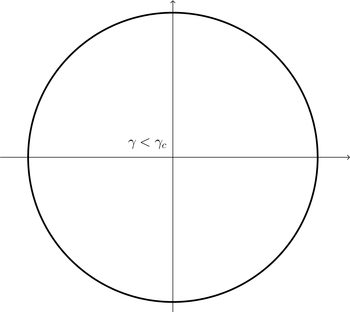
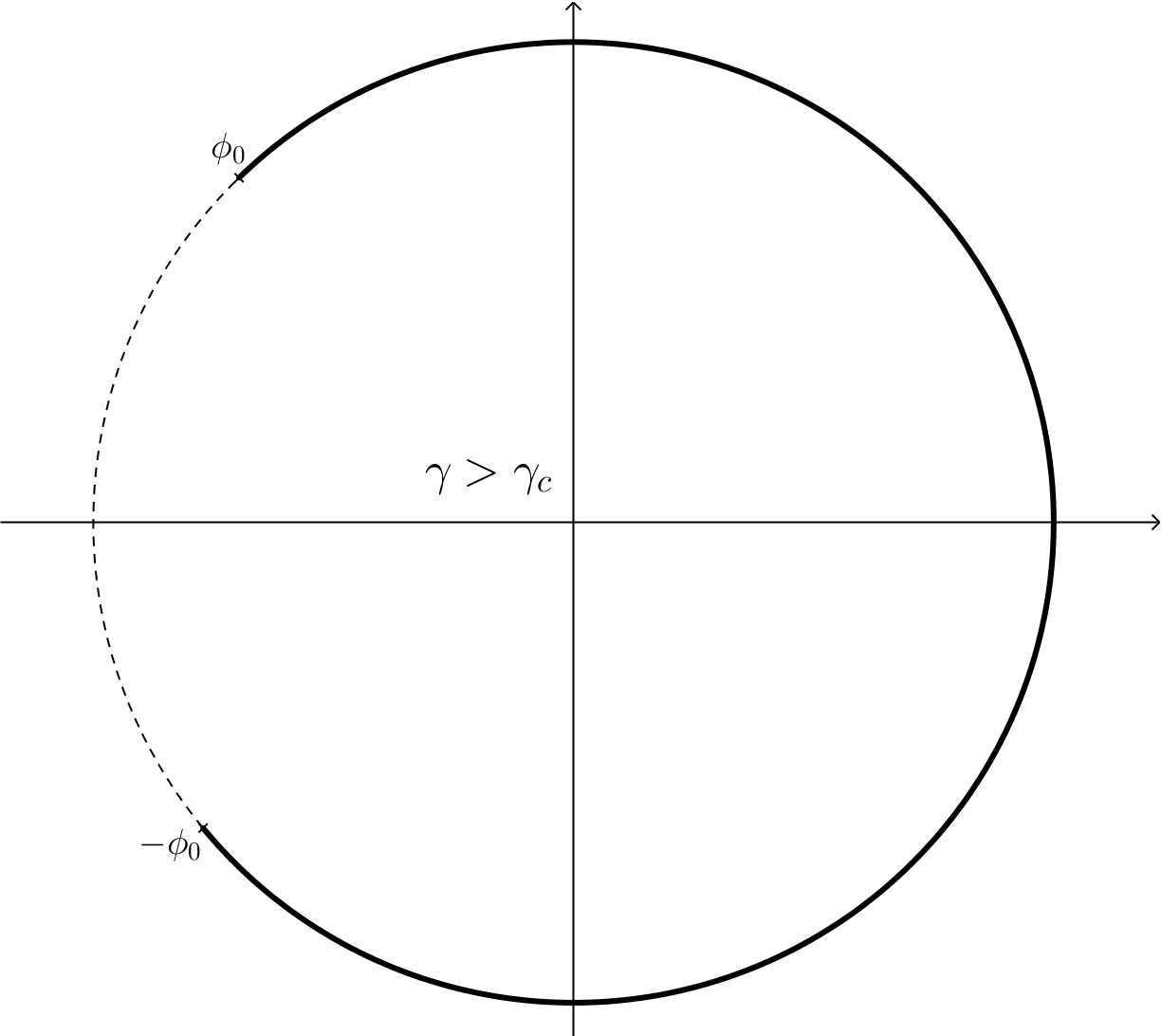
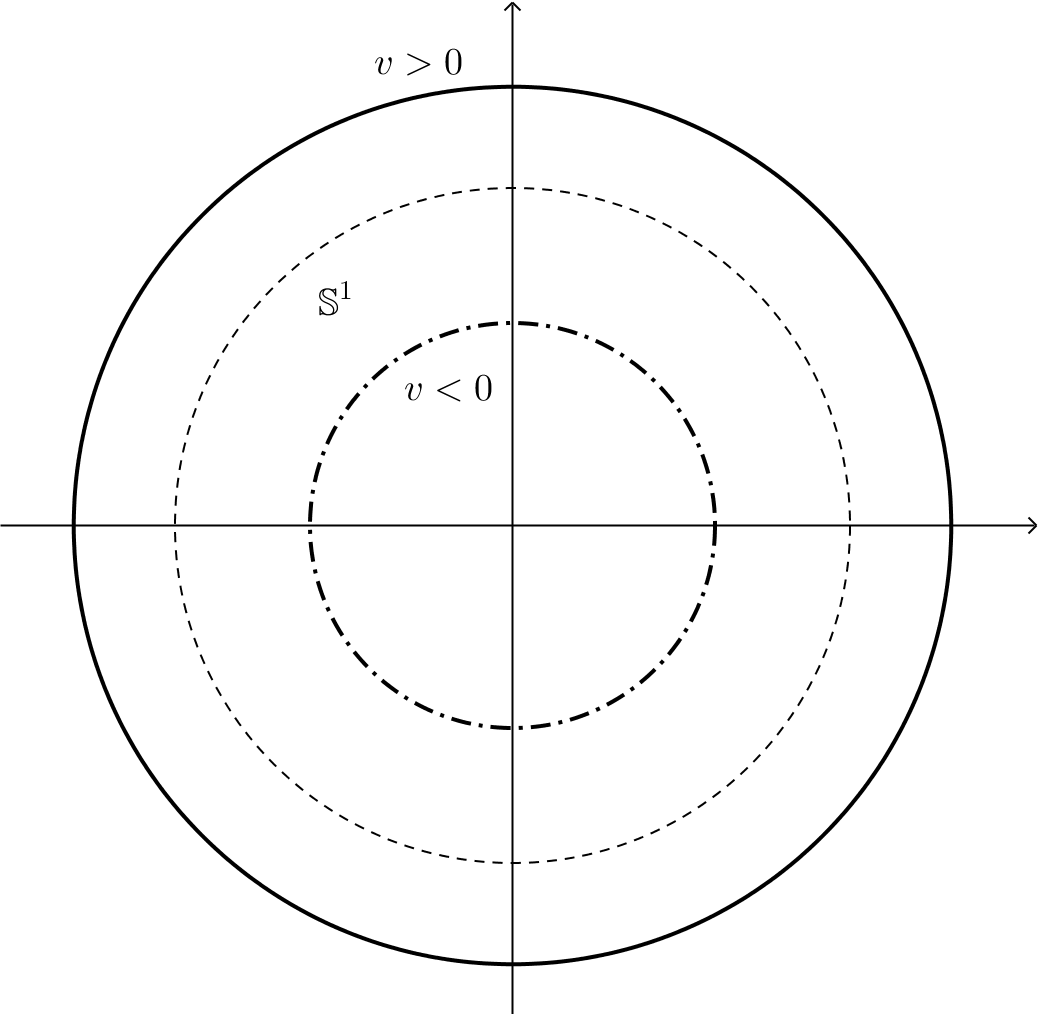
Our calculations are based on standard saddle point techniques, and we omit them from the main text and refer to the Appendices A and B. We will show that all the models undergo a phase transition when a gap opens in the support of the eigenvalue density, as schematized in Figure 1.
2.3. Phase transition: symmetric case
We first focus on the symmetric case , while the analysis of the more general case is undertaken later in Section 2.4.
Hence, the matrix models we analyze are:
| (2.6) | ||||
| (2.7) |
and we recall that admits an exact solution through the Cauchy identity, whilst does not. Nevertheless we have .
In [28], Baik proved that the first system, described by the partition function (2.6), and which we will call for simplicity the -model, undergoes a phase transition at large . We prove that the second system (2.7), which we call -model, undergoes the same phase transition. We prove it solving a singular integral equation in Appendix A, but in fact the result may also be directly obtained from [28], with minor changes.
2.3.1. The -model
Consider the matrix integral in (2.6), and take the limit with scaling as in (2.4). The leading contribution to comes from the solution to the system of saddle point equations that, with the help of the eigenvalue density as defined in (2.5), can be rewritten as a single singular integral equation:
| (2.8) |
where the symbol means principal value of the integral, and is the eigenvalue density for the specific model considered presently. The details of the solution to eq. (2.8) are spelled in Appendices A.1 and A.2. Two phases exists, separated by the critical curve [28]
The eigenvalue density, plotted in Figure 2 for various and , reads:
| (2.9) |
and allows to evaluate the free energy , obtaining:
| (2.10) |
where is -independent. See Appendices B.1 and B.2 for the calculation of the free energy. From the latter expression one sees that and are continuous functions for all values of , while
and therefore the system undergoes a third order phase transition at the critical curve .
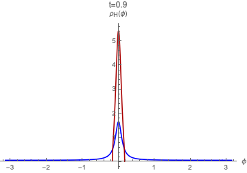
2.3.2. The -model
We now turn to the second matrix model, defined in eq. (2.7). The leading contribution in the large limit, with scaling (2.4), is obtained solving the saddle point equation
| (2.11) |
We solve this singular integral equation in Appendices A.3 and A.4. From direct comparison of the integral representation of and in (2.6) and (2.7), one would expect that, the solution to the second model is related to the solution to the first model by
Direct calculations prove that this is true and, in particular, the system undergoes a phase transition along the critical curve
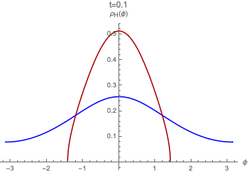
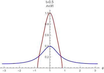
The eigenvalue density in the -model, plotted in Figure 3 for different values of and , is:
which allows to compute the free energy at large (see Appendices B.1 and B.2), and the final result is:
| (2.12) |
where is -independent. Taking derivatives, one finds again that first and second derivatives are continuous functions, while
thus the phase transition is of third order also in this case.
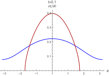
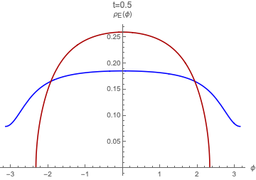
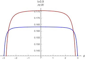
2.3.3. Double-scaling limit
We have shown that the free energy, and consequently the phase structure and the critical curve, of the matrix model with symmetric weight of type at large and large agrees with the equivalent descriptions as a Meixner ensemble with a hard wall studied in [9]. In fact, we find an even stronger agreement between the two pictures, as also the correlations among eigenvalues near the edge of the distributions in a double-scaling limit match. For the unitary ensemble, the double-scaling limit is described in [28], along the lines of [29]. On the other hand, in the discrete ensemble, if the critical region is approached from the small coupling phase, the hard wall is not active and the results of [24] directly apply. The double-scaling is the same in both cases, and leads to the Tracy–Widom law [30]. A third consistency check comes from the asymptotics of the hypergeometric kernel: standard computations using a steepest descend method (see for example [13, Sec. 4] for an introduction) show that the result in the double-scaling limit matches the Tracy–Widom behaviour.
2.4. Phase transition: general case
While in the previous Section 2.3 we focused on the analysis of two matrix models that are symmetric under , we now allow the more general situation , in which the symmetry is lost.
The matrix models we consider here are
| (2.13) | ||||
| (2.14) |
The weight functions are complex valued, thus we expect the eigenvalue densities at large to be complex-valued functions. We rewrite in terms of the parameters defined in (2.3), and consider the limit with scaling of as introduced in (2.4).
2.4.1. The -model
We first focus on the behaviour of the partition function (2.13) in the limit described above, and show how the discussion of the symmetric case in Section 2.3 is modified. Details of the calculations can be retrieved in Appendices A.5 and A.6 for weak and strong coupling respectively.
The leading contributions at large may be encoded in the eigenvalue density which solves the integral equation
| (2.15) |
The asymmetry parameter complexifies the left hand side of the latter equation, and the resulting eigenvalue density is complex (see Appendices A.5 and A.6):
with critical value , the same as in the symmetric case. The corresponding free energy , computed in Appendix B.3, can be written as:
| (2.16) |
The introduction of the asymmetry reduces the order of the phase transition from third to second, with:
2.4.2. The -model
Consider now the second matrix model, the -model of eq. (2.14), and take its scaled limit as in (2.3)-(2.4). The saddle point equation reads
| (2.17) |
The eigenvalue density is complexified by the presence of the asymmetry parameter (see Appendices A.7 and A.8):
with the same critical value as for the symmetric case: . The free energy is (see Appendix B.3):
| (2.18) |
The first derivative of the free energy is continuous, but the second derivative is not:
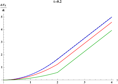
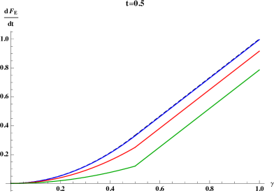
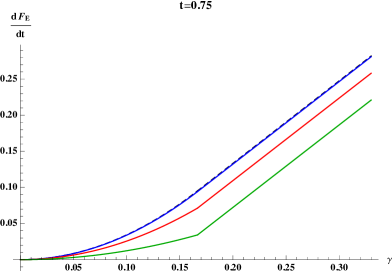
thus the phase transition is second order. We plot the first derivative of free energy as a function of , at different values of , in Figure 4.
2.5. The Gross–Witten limit
Consider the two matrix models of Section 2.3, defined in equations (2.6) and (2.7). The potential of those models can be written as:
with sign for the and for the . We send and , keeping their product fixed. This gives:
which is the potential of the Gross–Witten matrix model [31, 32]. Note that the limit is the same for both the - and the -model. In the more general, non-symmetric case, with potential
we pass from to as prescribed in (2.3), and define . The same limit as above gives:
which is the potential of the Gross–Witten model with a topological -term [33, 34]. Since, by construction, we are in the regime , the Gross–Witten phase transition is still present, as discussed in [34].
Within the setting laid down in the Introduction, the limit above with of the normalization of the -measure leads to the normalization of the Poissonized Plancherel measure on partitions [35, 16]. This is consistent with what we mentioned above, as the Poissonized Plancherel measure is mapped to the Gross–Witten unitary matrix model [36]. On the other side, the Poissonized Plancherel measure is the limit of the Meixner ensemble [37] as well.
2.6. Phase transition: from third to second order
For , the potential of the unitary matrix models (2.13)-(2.14) becomes complex-valued. We have studied the large limit and showed that the model undergoes a second order phase transition, which becomes third order turning off the asymmetry parameter, . Nevertheless, the phase transition in the Gross–Witten matrix model remains third order if the potential is modified into
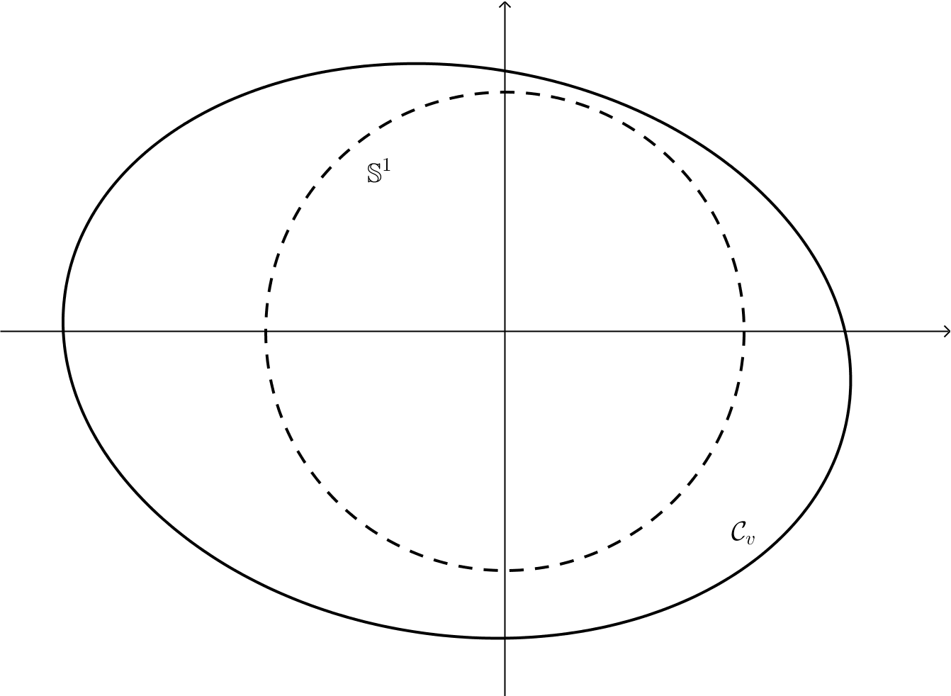
An alternative approach to face the matrix models with complexified potential is to analytically continue them in the sense of [38]. We relax the condition and deform the integration cycle in the complex plane so that the potential remains real along (see Figure 5). Of course, for the deformation to be smooth, should be a smooth Jordan curve, whose shape depends on and which is the unit circle when .
As a warm up, we apply the analytic continuation to the Gross–Witten model: we seek a contour such that
for all . We find that is simply a circle of radius . Moreover, the potential is
Hence, not only it is real-valued, but we also recover the original, symmetric Gross–Witten model sitting on a rescaled circle, see Figure 6. Furthermore, is sent to infinity or shrinks to a point as or respectively, and we cannot prolong beyond these values. This provides a new perspective on the result of [33, 34], where a drastic difference in the behaviour was observed crossing from to .
For a generic Laurent polynomial potential
the smooth integration cycle is determined as the locus in that solves the algebraic equation
Stated more formally, provided the potential is a Laurent polynomial, we determine a suitable contour as a rational algebraic curve of genus zero. If the curve has disconnected components, we simply retain as integration cycle the component homeomorphic to . Under the assumption that the coefficients are generic, this guarantees that the locus will be a small deformation of if is deformed by a small . See, for example, [39] for a textbook reference on affine algebraic curves.
However, the potentials of the matrix models with weights of and type are not polynomials but logarithms. The form of the potential is precisely the reason for the discontinuous behaviour as a function of , because then imposing
| (2.19) |
does not define an algebraic curve embedded in . For every real we find that the unique contour solving (2.19) is a half real line together with an open segment (the details depend on whether we consider the - or the -model), which is not a smooth deformation of .
It is perhaps instructive to look at the problem from the converse perspective. In general, the existence of a Jordan curve , depending on a collection of parameters , along which the potential is real-valued is not guaranteed. For non-polynomial potential , it requires to place the model at certain special points of the parameter space. For the weights of and type, this dictates , equivalently .
2.6.1. Phase transition and universality
To sum up our conclusions in one sentence, the unitary matrix models with symmetric and weight undergo a third order GW phase transition, but their more general, non-symmetric extensions have complex potentials and therefore fall out of the GW universality class. This ought to be contrasted with what happens in the equivalent description as a discrete ensemble with a hard wall. In that case, increasing the parameter from zero, the system undergoes a third order phase transitions at the value when the hard wall becomes active. This holds both in the symmetric and the more general setting: they belong to the same universality class. See [40, 41] for detailed discussion on the universality of the third order phase transition in presence of a hard wall. We also stress that the discrete topology further constrains the eigenvalue density, but the condition is satisfied for all values of the parameters [9, 10]. Thus, the discrete nature of the ensemble plays no role in determining the phase structure of this model.
It is worth mentioning that the symmetric -model has also been studied in the context of supersymmetric gauge theories, both with unitary [42] and orthogonal and symplectic symmetry [43], and the third order phase transition was observed also in the latter case [44]333The unitary matrix model of [42, Eq. (2.18)] corresponds to a generic choice , thus the weight function is complex. Setting in [42] combines chiral and anti-chiral matter fields: it would be interesting to interpret the change of order of the phase transition from second to third in that context..
3. Random matrix ensembles on the real line
We now discuss two random matrix models on the real line that follow from a change of variables of the unitary matrix models above described. One family of random matrix ensembles is obtained through the 1d stereographic projection, leading to a Cauchy–Romanovski type of ensembles and the other one is based on the mapping which is more useful when the original matrix model has a symplectic or orthogonal symmetry (that is, corresponding with ToeplitzHankel determinants, instead of Toeplitz determinants), but that also lead to explicit expressions for the symmetric unitary matrix models, in terms of Wronskians of Chebyshev polynomials of the four types.
3.1. Cauchy ensembles and Romanovski orthogonal polynomials
We analyse the matrix models and defined in eq. (2.6) and (2.7) and consider a change of topology, in which we remove a single point from the unit circle, to obtain . We expect the asymptotic behavior of these models at large to correspond to the “gapped” phase of the unitary matrix model (see Figure 1), which appears at strong coupling. We pass from angular variables to the real line using the stereographic projection [2, Sec. 2.5]:
as sketched in Figure 7.
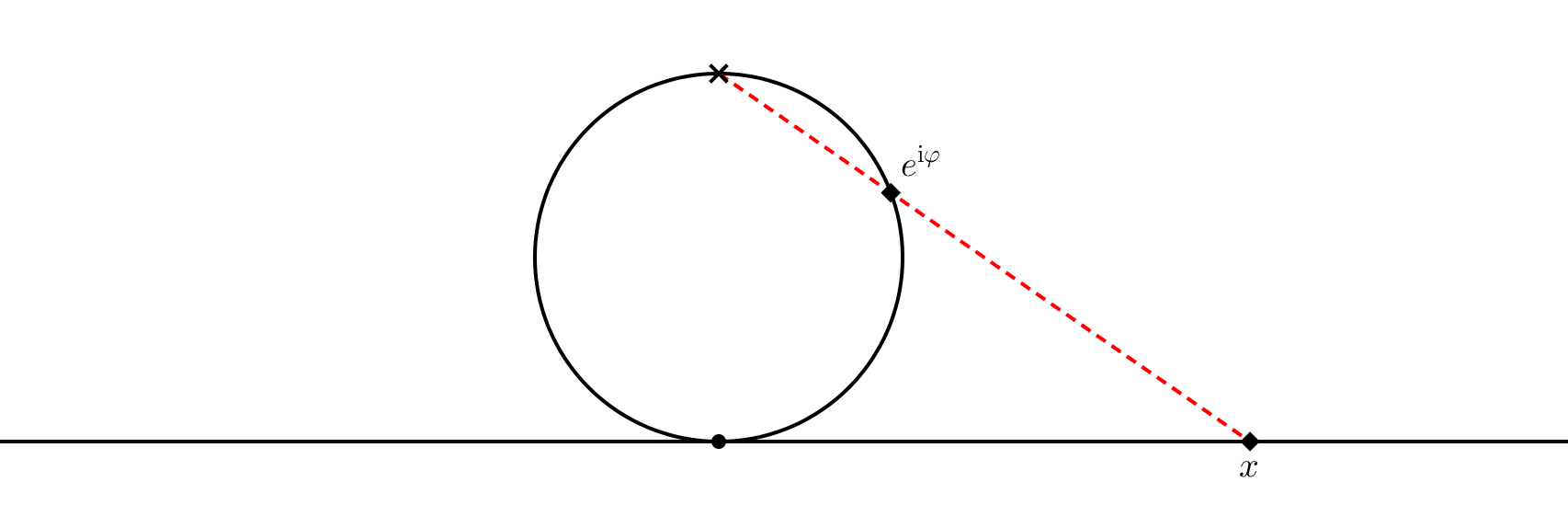
The Vandermonde determinant is mapped to:
and, with the corresponding transformation of the symbols, the resulting matrix models are:
| (3.1) | ||||
| (3.2) |
Likewise, we can also use the stereographic projection in the more general, non-symmetric, matrix models (2.13) and (2.14). We obtain:
| (3.3) | ||||
| (3.4) |
where we used the redefinition of parameters and .
3.1.1. Exact evaluation
In the limit case , the partition function of the symmetric -model, after stereographic projection, takes the simple form:
| (3.5) |
This random matrix ensemble has been studied as a Cauchy ensemble [45], Lorentz ensemble [46], and in this form it is a particular case of the classical ensemble with weight [2, 47]
This weight function satisfies the Pearson equation and hence the associated random matrix ensemble is classical [47, 48, 2], although in many references the listing of classical ensembles appears restricted to Hermite, Laguerre and Jacobi. See e.g. [48] for the expanded list of possible classical weights. The associated polynomials go under many names, including pseudo-Jacobi [49, 50, 51, 52, 53] due to their (non-trivial) relationship with Jacobi polynomials, and also appear in [54]. A proper name seems Romanovski polynomials given [55, 49], see [56] for a review. We evaluate now the matrix integral (3.5) using Romanovski polynomials. They satisfy (the dependence on is understood):
where we have chosen a normalization such that the polynomials are monic, and their norm squared is [57]
where the second square bracket is the change of normalization to obtain monic Romanovski polynomials from the normalization of [57]. Therefore, using
with specialized to the case of interest , we obtain
where the Barnes -function [17] is identified using
The result is the same indeed as eq. (2.1). Therefore, the is computed in three different ways: as a discrete ensemble on a finite set, as a unitary ensemble, and as the Cauchy ensemble on the real line. The tools used in each of the three approaches are, respectively: the Hahn polynomials [10], the Toeplitz determinant with symbol with a pure Fisher–Hartwig singularity [25], and the Romanovski polynomials, as represented in Figure 8.
3.1.2. Asymmetric Toeplitz matrix
A much studied symbol in spectral analysis of Toeplitz matrices [58, 59] is
| (3.6) |
for integer . As discussed in Section 2.1, this has the effect of shifting the Fourier coefficients of the symbol by , thus it shifts the diagonals of the Toeplitz matrix upward (if ) or downward () by and the Toeplitz banded matrix associated to our model becomes asymmetric, making it more similar to the generalized model in terms of this asymmetry of the associated Toeplitz matrix. The stereographic projection of this extra term is:
For , the resulting weight function is
| (3.7) |
This is the stereographic projection of the weight introduced in eq. (2.2), and it is still of the Romanovski form (see [47]) with the identification
We can therefore give explicit evaluation of the determinant of the Toeplitz banded matrix with symbol (3.7) using again Romanovksi polynomials:
| (3.8) |
Note that, if we consider the random matrix ensemble with weight (3.7) and keep the normalization such that it coincides with the stereographic projection of the unitary ensemble with weight (2.2), discussed in Section 2.1, the factor in bracket in (3.8) cancels exactly.
3.2. Large limit
We now focus on , in eq. (3.2), and study its large limit, with fixed. The saddle point equation is:
| (3.9) |
The parity symmetry of the matrix model guarantees that we can look for a symmetric solution with , . We expect that will be back-projected to of Section 2.3 undoing the stereographic projection.
We report the details of the computations in Appendix C.1. We arrive to the eigenvalue density:
with the boundary fixed by normalization:
This solution is well defined as long as
and sending , which would be back-projected to , corresponds to the limit . This matches the analysis on the circle.
We can do the same with the more general matrix model of eq. (3.4). In this case, as happened on the circle, turning on the asymmetry parameter complexifies the eigenvalue density, which becomes:
with same value of as above. The derivation of the result is given in Appendix C.2. For completeness, we also report the details of the large analysis of the matrix model with weight (3.6), corresponding to the determinant of an asymmetric Toeplitz matrix, in Appendix C.3.
3.3. Orthogonal and symplectic symmetries and Wronskians of Chebyshev polynomials
The other option, to pass from the unit circle to the real line, is to use . This works best for matrix integrals where the Haar measure is that of , or . That is, for ToeplitzHankel determinants. In that case the result [60, Lemma 2.7] holds, connecting ToeplitzHankel and Hankel determinants.
Lemma 3.1 ([60]).
Let be the Fourier coefficient of the symbol , , with444The symmetric symbols of and type satisfy the assumption, but the non-symmetric symbols do not. . Then,
where is the Hankel determinant on , with .
We give a new proof of this result following [61]. First, we set the notation for the rest of the Section. Denote the real orthogonal matrices with determinant , and
Note that the Haar measures on and coincide. Let us consider matrix integrals with weight over the group (see [2, Sec. 2.6] for details on the Haar measure on orthogonal and symplectic groups), which we denote by .
Proof of Lemma 3.1.
The change of variable gives
| (3.10) |
with depending on the symmetry of the original model,
| (3.11) |
|
and the overall normalization depends on the specific :
Using Andréief’s identity [22, 23], expression (3.10) gives the four Hankel determinants on the right hand sides in the Lemma, according to the choice of . The ToeplitzHankel determinants on the left hand sides in the Lemma correspond with matrix integration over orthogonal and symplectic group [62, 61]. Indeed, for
Furthermore, as noted in [61],
but then we have
This concludes the proof of the four identities. ∎
For the case of the symmetric and symbols considered in the paper, we have expressions of the general form:
| (3.12) |
with and as in (3.11). The signs are always the upper sign for the -model and the lower for the -model. Moreover, we take a positive integer. Thus, are averages of moments of characteristic polynomials, taken in a random matrix ensemble where the weight function is of the Jacobi type, , but always with the specific values of and above, corresponding to the Chebyshev subfamily. Hence, the corresponding orthogonal polynomials for
are Chebyshev polynomials of first, second, third and fourth kind respectively, denoted by
Their correspondence with group integration is (3.11). As mentioned, instead of interpreting the resulting model (3.12) as the partition function of a model with a semi-classical weight function (which in itself is an interesting possibility and may lead to connections with Painlevé equations and other integrable models), we adopt the characteristic polynomial point of view [63, 64], which, for the sign case in (3.12) (below we discuss the other choice), gives that
where denotes the Wronskian determinant and denotes one of the four Chebyshev polynomials. We also have defined the coefficients
( is for later use). The result follows immediately from Lemma 3.1 above (i.e. [60, Lemma 2.7]) together with the known characteristic polynomial results [63]. It has also been the specific subject of a later paper [65], where the same result is obtained, for a polynomial and, as above, even, symbol. Therefore it holds that:
In addition, we can also study the case with symbol in the same manner. For negative moments the characteristic polynomial description becomes involved, having to consider not the polynomials orthogonal w.r.t. the given weight, but the Cauchy transform of these polynomials [64]. In some cases this is a considerable complication, however, for Chebyshev polynomials, it is well known that the polynomials of first and second kind (and likewise the polynomials of third and fourth kind) are integral transforms of each other with respect to weighted Hilbert kernels [66]:
with the Cauchy principal value integral. The weighting is precisely the corresponding weight function, which is how it is required [64]. Note also that for , thus falls outside the integration region: in this case the Hilbert and Cauchy transform simply differ by a factor . Therefore, when we have:
Thus, we obtain a duality between the model with and the model with and conversely. The parameters are mapped , under the duality. We also obtain a tight relation between the model with and the model with and conversely, although it is not really a duality in the sense that we cannot recover one result from the other via a bijective map of the parameters.
So far, we have discussed the same models as above but with a symplectic or orthogonal symmetry (it would be interesting if such model had an interpretation in terms of a dimer problem, perhaps with boundaries, but we do not know of such an interpretation). The unitary case follows from the identity [67]:
which is used in matrix integral form in [61] and was used in [68] to precisely extend the Wronskian result [65] (again for a symbol of the type) to the unitary case. Therefore, from this Wronskian point of view, the unitary matrix model is more complicated than the orthogonal and symplectic ones, because it is the product of two Wronskians. The formulas for the symmetric symbol are555Note that in the odd case the two Wronskians correspond to and , not .:
and for the symbol
with coefficients
We obtain a duality for with and symbol, with parameters mapped according to and together with the factor in the -model. The relation between the model with and symbol and group is not a duality.
It is worth mentioning that Wronskians of orthogonal polynomials in general satisfy an interesting identity which expresses them as Hankel determinants, but with the roles of the and swapped [69]. In the case of the Chebyshev Wronskian of the first type, the Hankel determinant is in terms of Legendre polynomials and for the second type one is in terms of a Hankel of Gegenbauer polynomials (polynomials orthogonal w.r.t. ).
3.3.1. Large limit
The asymptotics of a Hankel determinant with symbol , with and Lipschitz continuous, has been obtained by Basor and Chen [70] when . They also showed that the resulting expression can be analytically continued to all , and therefore it applies to the matrix ensemble (3.12) for each of the four symmetry groups. In that case, and , with upper sign for the model and lower sign for the model. Recall also that , hence is admissible in both models. The formula of [70] for generic and is:
| (3.13) |
for large , where is independent of and is given by:
This expression directly gives the asymptotic behaviour of for both symbols. First, we notice that the numerical prefactor in (3.12) simplifies with the one coming from formula (3.13), exactly for and leaving behind a factor of when . Then, we use
and see that the contribution from the exponential in (3.13) cancels:
We are left with the contribution from . The ratio of products of Barnes -functions and the Gamma function is trivial for , and is for , thus cancelling the left over factor from the numerical coefficient. The exponential of the single integral gives
and in particular is trivial for odd rank symmetry, . The double integral which appears in the exponential in is universal for the four symmetries and takes the form
The last integral admits an exact solution in terms of hypergeometric functions, albeit involved. Instead, we write explicitly as and, using , we expand the logarithm:
After integration the term cancels, while for we use the Hilbert transform property of the Chebyshev polynomials to arrive at the final expressions
with upper sign for the -model and lower sign for the -model. Note that we cannot recast the series into a logarithm because .
We obtained the large limit with fixed , but we could also study the large and large limit with fixed, as we did in Section 2.3 for the matrix models with unitary symmetry. This scaled limit was analyzed in [44] (except for , which is nonetheless easily found following their argument), and a third order phase transition from a gapless to a gapped phase was observed, in agreement with the results in the unitary setting.
4. Outlook
It would be interesting if semiclassical polynomials can be used to obtain further analytical results on the model with orthogonal and symplectic symmetries, using the Wronskian representation presented here. Notice that computing these Wronskians is equivalent to computing determinants of banded matrices of the ToeplitzHankel type, which arise for example as Laplacian or difference matrices of problems with boundaries [71, 72].
Other analytical approaches could have been followed as well. For example, it is immediate to interpret (3.2) as a characteristic polynomial average over a Cauchy ensemble666Note that because the arguments of the polynomials would be purely imaginary, the determinantal expressions would be in terms of Jacobi polynomials, for this model.. It would be more interesting to use this approach for the case of the asymmetric symbol (3.6), which, when mapped on the real line, gives the full Cauchy–Romanovski weight. This could be studied in the context of asymmetrically banded Toeplitz matrices.
At large , it could be interesting to consider the recent results [73] on correlators of characteristic polynomials for classical ensembles. If a confluent limit of these results on correlators can be taken, that would directly evaluate the Wronskian description of the orthogonal and symplectic ensembles discussed in Section 3.3. On the other hand, the asymptotic formulas in [73] already could be directly applied to a -deformation of the -model, such as the one studied in [21, Sec. 4.3].
It is worth mentioning that the Cauchy ensemble has interesting connections with the Laguerre ensemble and Painlevé equations [74, 75] that may be further exploited in our context. We could also focus further on the exact equivalences part and see if other averages over the Meixner ensemble, such as the ones in [76], have a counterpart in terms of the and unitary random matrix ensembles.
With regards to the phase structure, it seems also worth exploring if the phase transitions obtained, which are phase transitions of the determinant in the Toeplitz matrix representation of the and models, are related to any spectral change of the Toeplitz matrices, which in the case of the -model is a banded matrix. The spectra of such matrices is still of very much interest and a rich subject [58, 59] and it could be a worthwhile direction to study the spectra in the natural scaling limit suggested by the random matrix representation, the one explored here.
We conclude by mentioning that passing from a third order to a second order phase transition opens up the possibility of intriguing interpretations. According to [77], the negative jump of the second derivative of the free energy when crossing the critical line is associated with the creation of a meta-stable state, and the second order phase transition corresponds to tunneling from the meta-stable vacuum to the stable one. This aspect may deserve further attention.
Acknowledgements
The work of MT was partially supported by the Fundação para a Ciência e a Tecnologia (FCT) through its program Investigador FCT IF2014, under contract IF/01767/2014. The work of LS is supported by the FCT through the doctoral grant SFRH/BD/129405/2017. The work is also supported by FCT Project PTDC/MAT-PUR/30234/2017.
Appendix A Solution to saddle point equations on the unit circle
Here we present the calculations to solve the saddle point equations obtained in the scaled large size limit of the unitary matrix models discussed in Section 2.
A.1. Solution for at weak coupling
We start with the solution of the saddle point equation (2.8), which we rewrite here for completeness:
| (A.1) |
The solution was originally obtained by Baik in [28], and the present derivation via saddle point equations was discussed in [78].
We make the ansatz . On the right hand side of (A.1) we use the expansion (for ):
thus the integration extracts the Fourier coefficients of the eigenvalue density:
where
For the left hand side we use:
where in the second equality we recognized the generating function of Chebyshev polynomials of second kind, . Exploiting the basic property , equation (A.1) is rewritten as:
and we immediately get:
| (A.2) |
for all . The only yet undetermined coefficient is fixed by normalization to . Putting all together:
which can be further simplified recognizing the generating function of Chebyshev polynomials of first kind , using the property . We finally arrive to:
| (A.3) |
The minima of this function are located at , and imposing the condition for all , we see that the present solution holds in the regime
Above the critical value , solution (A.3) ceases to be valid and we must drop the assumption and look for a different solution.
A.2. Solution for at strong coupling
In this Appendix we present the calculations to solve the saddle point equation (2.8) at strong coupling. The procedure follows [79, App. B] (see also [78, Sec. 4]). We look for a one-cut solution with , .
We introduce the following complex function, named resolvent:
Here, is the arc of the unit circle from to , oriented anti-clockwise, and the complex function is the continuation of to the complex plane, with . The eigenvalue density is recovered from the resolvent through the relation
with the subscript (resp. ) meaning the limit taken from outside (resp. inside) the unit circle.
Following standard methods, we introduce two auxiliary complex functions:
| (A.4) |
and a function , to be determined, such that
| (A.5) |
The saddle point equation (2.8) becomes a discontinuity equation for . We will use this discontinuity equation, together with the fact that, by definition, decays as as , to obtain an integral expression for (see [79, 78]). Explicitly:
where we denoted for shortness the left hand side of eq. (A.1), and the contour encloses the branch cut , the arc along the unit circle. See Figure 9.
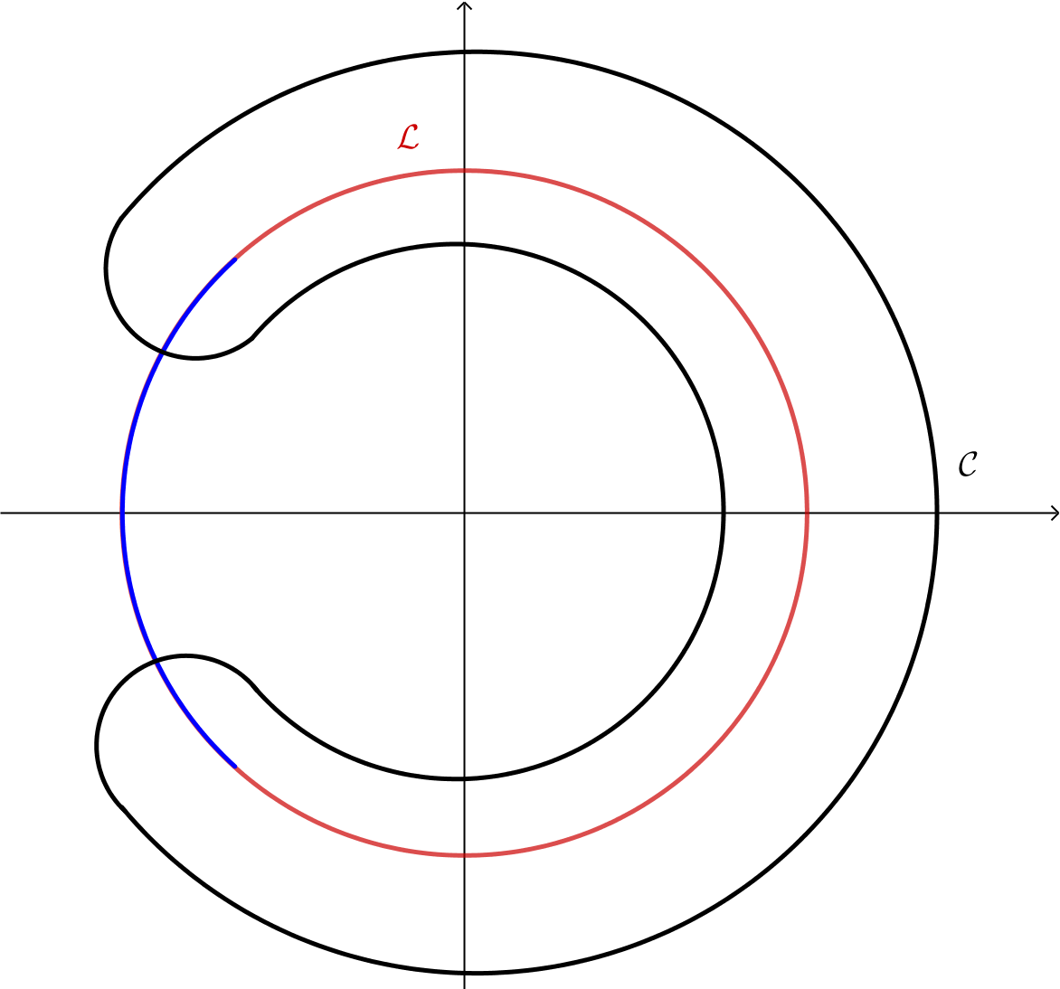
At this stage, we notice that the left hand side of eq. (A.1) has poles but no branch cuts, so we can manipulate the integration contour in a convenient way. We arrive to:
where the three contributions are:
The sum in runs over the poles of the derivative of the potential (that is, the poles of the left hand side of eq. (A.1)), in this case , and is a large circle of radius . We have and yields no discontinuity, so it is irrelevant for the evaluation of . The unique relevant contribution comes from:
| (A.6) | ||||
where for the last equality we used . In general, on the real axis if and if . Therefore, since , we bare in mind that .
Plugging the expression for into and taking its discontinuity along the arc , we arrive to:
| (A.7) |
The boundary of the support is fixed by normalization:
which provides
and hence, writing explicitly, we obtain:
Also, plugging the expression for in (A.7), we arrive to the final expression
A.3. Solution for at weak coupling
In this Appendix we solve the saddle point equation (2.11), which we rewrite here for completeness:
| (A.8) |
The analysis will follow closely Appendix A.1 for small coupling and Appendix A.2 for strong coupling, and we omit most of the details.
We again start with the ansatz , and manipulate the right hand side of (A.8) exactly as we did in Appendix A.1, and for the left hand side we use:
Then, eq. (A.8) becomes
with the Fourier coefficients of , and we immediately obtain:
where, as usual, is fixed by normalization. We recognize the generating function of Chebyshev polynomials of the first kind, using the standard identity , and arrive to the final expression for the eigenvalue density
The minima are placed at , and the non-negativity condition holds as long as:
We see that, as expected by naïve comparison of the integral representation of the matrix models (2.6) and (2.7), the eigenvalue densities and , as well as the respective critical points, are related through .
A.4. Solution for at strong coupling
The procedure at strong coupling is as in Appendix A.2, and we avoid the technical details here. We assume a one-cut solution supported on , , and introduce the resolvent
with integration contour meant to be the arc along the unit circle connecting to , and the function being the continuation of in , with . We introduce, as in Appendix A.2, the complex functions and , and the saddle point equation (A.8) becomes a discontinuity equation for . The only relevant contribution (for the computation of ) to is:
where for the last equality we used , with both understood to be negative. We get:
| (A.9) |
and is fixed by the normalization:
Thus,
Combining this latter expression with eq. (A.9), we finally arrive to:
supported in .
A.5. Solution for at weak coupling
This Appendix is dedicated to the solution, in the weak coupling regime, to the saddle point equation (2.15), which we rewrite here for convenience:
| (A.10) |
The procedure is similar to the one adopted in Appendix A.1, but now the parameter makes the left hand side complex-valued. Therefore, we expand the eigenvalue density in the exponential form:
while we also use777The expression holds for , which is guaranteed by the principal value of the integral.:
The right hand side of (A.10) then becomes:
For the left hand side we can expand the geometric series and obtain:
Putting all together, and taking into account the normalization condition that fixes , we arrive to:
We see that the parameter , which controls the asymmetry, introduces an imaginary part in the eigenvalue density. Since , the relevant minima are those of the real part, thus the critical value is the same as in the symmetric case:
and above this value the solution ceases to be valid.
A.6. Solution for at strong coupling
When we have to look for a different solution to the saddle point equation (A.10). At strong coupling, the procedure is exactly the same as in Appendix A.2, since we were already working in the complex plane, so the complexification of the left hand side of eq. (A.10) for does not alter the strategy. We assume a gapped one-cut solution supported on and introduce the resolvent
Everything goes trough exactly as in Appendix A.2, except for the factors of appearing in the left hand side of eq. (A.10). One easily finds:
The normalization fixes , through:
Notice that, due to the parity of the integral, the result is independent of , in particular it is equal to the symmetric case (). The final expression for the eigenvalue density:
with the same as in [28] and Appendix A.2, that is
A.7. Solution for at weak coupling
Here we solve the large limit of the second matrix model, eq. (2.14), in the general case. The saddle point equation (2.17) is:
| (A.11) |
The procedure is as in Appendix A.5. The right hand side reads:
while, expanding the geometric series, the left hand side becomes:
This gives:
Again, the validity of this solution extends up to:
as in the symmetric case.
A.8. Solution for at strong coupling
When , we drop the assumption and look for a one-cut solution with a gap. The procedure is clear from the previous Appendices, and the result is:
which, after imposing normalization and rewriting in terms of trigonometric functions, gives:
supported on
Appendix B Free energies
This Appendix contains the calculations to obtain the free energy of the unitary matrix models considered in the main text.
B.1. Free energy for and at weak coupling
The simplest way to obtain the free energy is to evaluate its derivative with respect to the parameter and then integrate. In the weak coupling phase, , we can use the boundary condition , which follows immediately from the normalization of the Haar measure on . At strong coupling we use the continuity of at .
For what concerns , at weak coupling we have:
Integrating with boundary condition gives
| (B.1) |
For at weak coupling we have:
which, after integration, gives
| (B.2) |
In particular, we see that the free energies of the two models are equal in the weak coupling phase. This is expected, since, in the weak coupling phase, the free energy equals the result provided by Szegő theorem, i.e. the limit without scaling (see e.g. [78] for a proof of this statement), and it is well known that the limits of the models (2.6) and (2.7) without scaling are equal.
B.2. Free energy for and at strong coupling
We now pass to the strong coupling phase, and use the form of the eigenvalue densities and at .
Starting with , we have:
where we used the change of variables and used the explicit form of . Immediate integration gives:
with a -independent integration constant fixed by continuity at .
For the calculations are almost the same, except for the change of sign in front of all factors of and . We get:
Notice that the final line here could not be inferred from the final line of with reversed signs. After integration we obtain the result:
| (B.3) |
where is -independent and fixed by continuity at the critical value .
B.3. Free energy for and
The free energies for the matrix models (2.13) and (2.14) are computed at weak coupling in exactly the same manner as in Appendix B.1. It is easy to check that, thanks to the parity of the integral, the free energies receive contribution from the terms proportional to but they remain real. Direct computations give:
At strong coupling we get:
where in the second line we changed variables , with boundary at , and in the last line we used the explicit form of to simplify the resulting expression. Notice that the term proportional to does not depend explicitly on .
Following the same steps, the free energy is computed at strong coupling as:
Appendix C Solution to the saddle point equations on the real line
Here we consider the solution to the saddle point equation obtained from the large limit of the matrix model after stereographic projection on the real line, as described in Section 3.2. We focus on and , and the solutions for the -models can be obtained in an analogous way.
C.1. Solution for
We consider first the matrix model defined in eq. (3.2). In the limit in which the number of variables, , is large, the leading contribution comes from the eigenvalue density that solves the saddle point equation (3.9), which we report here for convenience:
| (C.1) |
with
We proceed following standard methods for the analysis of Hermitian matrix models at large , as reviewed for example in [80]. We introduce the resolvent
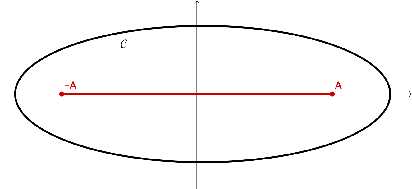
where now, assuming a solution with symmetric support , the path is the segment on the real line. The eigenvalue density is recovered as the jump of the resolvent along :
with meaning the limit taken approaching the real line from the upper (resp. lower) half plane.
A solution for the resolvent is the following: write
and the saddle point equation (C.1) becomes a discontinuity equation for , with solution:
where the contour is a closed curve surrounding the cut , as in Figure 10.
is a meromorphic function, with simple poles at:
We can thus deform the contour, to avoid the branch cut of the square root, and pick the poles of the integrand. This leaves a residual integral along an infinitely large circle. This latter contribution vanishes, since at large . The pole at generates the regular part of , thus yields no contribution to the eigenvalue density. Therefore, the relevant contributions to the arise from the poles of in the complex plane. For the calculations, one has to be careful with the signs in front of the square roots, according to the definition of . With our conventions,
After simple computations, one arrives to:
The eigenvalue density is obtained this function multiplied by the jump of :
The value of the boundary can be fixed by normalization, or equivalently looking at the large behaviour of the resolvent . From the definition, one has , as , while from the explicit evaluation, we have:
This provides the solution (recall that )
This is a positive quantity, and thus is supported on the real line, as long as
This is consistent with our general analysis: due to the change of topology, the stereographic projection should only provide the gapped phase of the unitary matrix model. We also notice that, undoing the stereographic projection, we obtain:
thus the boundary we obtain on the real line is in fact the stereographic projection of the boundary of the model on the unit circle, as expected.
C.2. Solution for
In this Appendix, we study the large limit of the matrix model defined in eq. (3.4). The saddle point equation is:
| (C.2) |
with in the present, more general case given by:
From this expression, it is clear that the asymmetry in the integrand introduces an imaginary part in the eigenvalue density, but does not introduce new poles of in the complex plane.
We proceed as in the previous Appendix, and find:
where now the residues at yield an extra term, proportional to the parameter . After some simple calculations, we see that this extra contribution is:
The final expression for the eigenvalue density is:
Imposing normalization, from the parity of the integral we obtain the same value of as above.
C.3. Solution for with modified symbol
We now solve the saddle point equation (C.1) with, on the right hand side, the modified function
The procedure follows closely that of Appendix C.1, but now we do not assume symmetry of the support for , and let
We therefore modify the definition of the auxiliary function
For later convenience, we also introduce the functions
| (C.3) | ||||
for . Note also that and . Following Appendix C.1, we introduce the resolvent and arrive to:
with poles at . Using
and similarly for , we arrive to:
and the eigenvalue density is:
for . The boundaries of the support are fixed by imposing the condition at large . Using
order in the expansion of gives the constraint
while from order , and using the previous expression to simplify the equation, we get the constraint
References
- [1] M. L. Mehta, Random Matrices, Pure and Applied Mathematics. Elsevier Science, 2004.
- [2] P. J. Forrester, Log-gases and random matrices, vol. 34 of London Mathematical Society Monographs Series. Princeton University Press, Princeton, NJ, 2010, 10.1515/9781400835416.
- [3] G. Blower, Random Matrices: High Dimensional Phenomena, London Mathematical Society Lecture Note Series. Cambridge University Press, 2009, 10.1017/CBO9781139107129.
- [4] G. W. Anderson, A. Guionnet and O. Zeitouni, An Introduction to Random Matrices, Cambridge Studies in Advanced Mathematics. Cambridge University Press, 2009, 10.1017/CBO9780511801334.
- [5] G. Akemann, J. Baik and P. Di Francesco, The Oxford Handbook of Random Matrix Theory, Oxford Handbooks in Mathematics. Oxford University Press, 2011.
- [6] L. Pastur and M. Shcherbina, Eigenvalue distribution of large random matrices, vol. 171 of Mathematical Surveys and Monographs. American Mathematical Society, Providence, RI, 2011, 10.1090/surv/171.
- [7] T. Tao, Topics in random matrix theory, vol. 132 of Graduate Studies in Mathematics. American Mathematical Society, Providence, RI, 2012, 10.1090/gsm/132.
- [8] J. Baik, P. Deift and T. Suidan, Combinatorics and random matrix theory, vol. 172 of Graduate Studies in Mathematics. American Mathematical Society, Providence, RI, 2016.
- [9] F. Colomo and A. G. Pronko, Third-order phase transition in random tilings, Phys. Rev. E88 (2013) 042125 [1306.6207].
- [10] F. Colomo and A. G. Pronko, Thermodynamics of the Six-Vertex Model in an L-Shaped Domain, Commun. Math. Phys. 339 (2015) 699 [1501.03135].
- [11] I. G. Macdonald, Symmetric Functions and Hall Polynomials, Oxford classic texts in the physical sciences. Clarendon Press, 1998.
- [12] A. Okounkov, Infinite wedge and random partitions, Selecta Math. (N.S.) 7 (2001) 57 [math/9907127].
- [13] A. Okounkov, The uses of random partitions, in XIVth International Congress on Mathematical Physics, pp. 379–403. World Sci. Publ., Hackensack, NJ, 2005. [math-ph/0309015].
- [14] A. Borodin and G. Olshanski, Distributions on partitions, point processes, and the hypergeometric kernel, Comm. Math. Phys. 211 (2000) 335 [math/9904010].
- [15] A. Okounkov, and -measures, in Random matrix models and their applications, vol. 40 of Math. Sci. Res. Inst. Publ., pp. 407–420. Cambridge Univ. Press, Cambridge, 2001. [math/0002135].
- [16] A. Borodin and G. Olshanski, -measures on partitions, Robinson-Schensted-Knuth correspondence, and random matrix ensembles, in Random matrix models and their applications, vol. 40 of Math. Sci. Res. Inst. Publ., pp. 71–94. Cambridge Univ. Press, Cambridge, 2001. [math/9905189].
- [17] E. Barnes, The theory of the g-function, Quart. J. Math. 31 (1899) 264.
- [18] J.-M. Stéphan, Extreme boundary conditions and random tilings, [2003.06339].
- [19] K. Johansson, A multi-dimensional markov chain and the meixner ensemble, Ark. Mat. 48 (2010) 79 [0707.0098].
- [20] K. Hikami and T. Imamura, Vicious walkers and hook Young tableaux, J. Phys. A 36 (2003) 3033 [cond-mat/0209512].
- [21] D. García-García and M. Tierz, Toeplitz minors and specializations of skew Schur polynomials, J. Combin. Theory 172 (2020) 105201 [1706.02574].
- [22] C. Andréief, Note sur une relation entre les intégrales définies des produits des fonctions, Mém . Soc. Sci. Phys. Nat. Bordeaux 2 (1886) 1.
- [23] P. J. Forrester, Meet Andréief, Bordeaux 1886, and Andreev, Kharkov 1882–-1883, Random Matrices: Theory and Applications 08 (2019) 1930001 [1806.10411].
- [24] K. Johansson, Shape fluctuations and random matrices, Comm. Math. Phys. 209 (2000) 437 [math/9903134].
- [25] A. Böttcher and B. Silbermann, Toeplitz matrices and determinants with Fisher-Hartwig symbols, J. Funct. Anal. 63 (1985) 178.
- [26] A. Böttcher and H. Widom, Two elementary derivations of the pure Fisher-Hartwig determinant, Integral Equations Operator Theory 53 (2005) 593 [math/0312198].
- [27] A. Böttcher and S. M. Grudsky, Spectral properties of banded Toeplitz matrices, vol. 96. Siam, 2005.
- [28] J. Baik, Random vicious walks and random matrices, Comm. Pure Appl. Math. 53 (2000) 1385 [math/0001022].
- [29] J. Baik, P. Deift and K. Johansson, On the distribution of the length of the longest increasing subsequence of random permutations, J. Amer. Math. Soc. 12 (1999) 1119 [math/9810105].
- [30] C. A. Tracy and H. Widom, Level spacing distributions and the Airy kernel, Commun. Math. Phys. 159 (1994) 151 [hep-th/9211141].
- [31] D. J. Gross and E. Witten, Possible Third Order Phase Transition in the Large N Lattice Gauge Theory, Phys. Rev. D21 (1980) 446.
- [32] S. R. Wadia, = Infinity Phase Transition in a Class of Exactly Soluble Model Lattice Gauge Theories, Phys. Lett. 93B (1980) 403.
- [33] M. Hisakado, Unitary matrix models and Painleve III, Mod. Phys. Lett. A11 (1996) 3001 [hep-th/9609214].
- [34] M. Hisakado, Unitary matrix models with a topological term and discrete time Toda equation, Phys. Lett. B395 (1997) 208 [hep-th/9611177].
- [35] A. Borodin, A. Okounkov and G. Olshanski, Asymptotics of Plancherel measures for symmetric groups, J. Amer. Math. Soc. 13 (2000) 481 [math/9905032].
- [36] K. Johansson, The longest increasing subsequence in a random permutation and a unitary random matrix model, Math. Res. Lett. 5 (1998) 63.
- [37] K. Johansson, Discrete orthogonal polynomial ensembles and the plancherel measure, Annals of Mathematics 153 (2001) 259 [math/9906120].
- [38] E. Witten, Analytic Continuation Of Chern-Simons Theory, AMS/IP Stud. Adv. Math. 50 (2011) 347 [1001.2933].
- [39] S. D. Cutkosky, Introduction to Algebraic Geometry, vol. 188 of Graduate Studies in Mathematics. American Mathematical Society, Providence, RI, 2018.
- [40] F. D. Cunden, P. Facchi, M. Ligabò and P. Vivo, Universality of the third-order phase transition in the constrained Coulomb gas, J. Stat. Mech. 1705 (2017) 053303 [1702.05071].
- [41] F. D. Cunden, P. Facchi, M. Ligabò and P. Vivo, Third-order phase transition: random matrices and screened Coulomb gas with hard walls, J. Stat. Phys. 175 (2019) 1262 [1810.12593].
- [42] Y. Chen and N. Mekareeya, The Hilbert series of U/SU SQCD and Toeplitz Determinants, Nucl. Phys. B850 (2011) 553 [1104.2045].
- [43] E. Basor, Y. Chen and N. Mekareeya, The Hilbert Series of and SQCD, Painlevé VI and Integrable Systems, Nucl. Phys. B860 (2012) 421 [1112.3848].
- [44] Y. Chen, N. Jokela, M. Jarvinen and N. Mekareeya, Moduli space of supersymmetric QCD in the Veneziano limit, JHEP 09 (2013) 131 [1303.6289].
- [45] N. S. Witte and P. J. Forrester, Gap probabilities in the finite and scaled Cauchy random matrix ensembles, Nonlinearity 13 (2000) 1965 [math-ph/0009022].
- [46] P. W. Brouwer, Generalized circular ensemble of scattering matrices for a chaotic cavity with non-ideal leads, Phys. Rev. B 51 (1995) 16878 [cond-mat/9501025].
- [47] W. Koepf and M. Masjed-Jamei, A generic polynomial solution for the differential equation of hypergeometric type and six sequences of orthogonal polynomials related to it, Integral Transforms Spec. Funct. 17 (2006) 559.
- [48] M. Masjed-Jamei, F. Marcellán and E. J. Huertas, A finite class of orthogonal functions generated by routh-romanovski polynomials, Complex Variables and Elliptic Equations 59 (2014) 162.
- [49] P. A. Lesky, Endliche und unendliche Systeme von kontinuierlichen klassischen Orthogonalpolynomen, Z. Angew. Math. Mech. 76 (1996) 181.
- [50] R. Koekoek, P. A. Lesky and R. F. Swarttouw, Hypergeometric orthogonal polynomials and their -analogues, Springer Monographs in Mathematics. Springer-Verlag, Berlin, 2010, 10.1007/978-3-642-05014-5.
- [51] K. Jordaan and F. Toókos, Orthogonality and asymptotics of pseudo-Jacobi polynomials for non-classical parameters, J. Approx. Theory 178 (2014) 1.
- [52] Z. Song and R. Wong, Asymptotics of pseudo-Jacobi polynomials with varying parameters, Stud. Appl. Math. 139 (2017) 179.
- [53] R. Wong, Asymptotics of orthogonal polynomials, Int. J. Numer. Anal. Model. 15 (2018) 193.
- [54] V. Aldaya, J. Bisquert and J. Navarro-Salas, The Quantum relativistic harmonic oscillator: Generalized Hermite polynomials, Phys. Lett. A156 (1991) 381.
- [55] V. Romanovski, Sur quelques classes nouvelles de polynomes orthogonaux, C. R. Acad. Sci. 188 (1929) 1023.
- [56] A. P. Raposo, H. J. Weber, D. E. Alvarez-Castillo and M. Kirchbach, Romanovski polynomials in selected physics problems, Central Eur. J. Phys. 5 (2007) 253 [0706.3897].
- [57] R. Askey, Beta integrals and the associated orthogonal polynomials, in Number theory, Madras 1987, vol. 1395 of Lecture Notes in Math., pp. 84–121. Springer, Berlin, 1989. DOI.
- [58] S.-E. Ekström, C. Garoni and S. Serra-Capizzano, Are the eigenvalues of banded symmetric toeplitz matrices known in almost closed form?, Experimental Mathematics 27 (2018) 478.
- [59] M. Barrera, A. Böttcher, S. M. Grudsky and E. A. Maximenko, Eigenvalues of even very nice Toeplitz matrices can be unexpectedly erratic, in The diversity and beauty of applied operator theory, vol. 268 of Oper. Theory Adv. Appl., pp. 51–77. Birkhäuser/Springer, Cham, 2018. [1710.05243]. DOI.
- [60] P. Deift, A. Its and I. Krasovsky, Asymptotics of Toeplitz, Hankel, and Toeplitz+Hankel determinants with Fisher-Hartwig singularities, Ann. of Math. (2) 174 (2011) 1243 [0905.0443].
- [61] D. García-García and M. Tierz, Matrix models for classical groups and ToeplitzHankel minors with applications to Chern-Simons theory and fermionic models, J. Phys. A in press (2020) [1901.08922].
- [62] J. Baik and E. M. Rains, Algebraic aspects of increasing subsequences, Duke Math. J. 109 (2001) 1 [math/9905083].
- [63] E. Brézin and S. Hikami, Characteristic polynomials of random matrices, Comm. Math. Phys. 214 (2000) [math-ph/9910005].
- [64] J. Baik, P. Deift and E. Strahov, Products and ratios of characteristic polynomials of random Hermitian matrices, J. Math. Phys. 44 (2003) 3657 [math-ph/0304016].
- [65] M. Elouafi, On a relationship between Chebyshev polynomials and Toeplitz determinants, Appl. Math. Comput. 229 (2014) 27.
- [66] J. C. Mason, Chebyshev polynomials of the second, third and fourth kinds in approximation, indefinite integration, and integral transforms, J. Comput. Appl. Math. 49 (1993) 169.
- [67] R. Vein and P. Dale, Determinants and their applications in mathematical physics, vol. 134 of Applied Mathematical Sciences. Springer-Verlag, New York, 1999, 10.1007/b98968.
- [68] M. Elouafi, A Widom like formula for some Toeplitz plus Hankel determinants, J. Math. Anal. Appl. 422 (2015) 240.
- [69] B. Leclerc, On certain formulas of Karlin and Szegö, Sém. Lothar. Combin. 41 (1998) Art. B41d, 21.
- [70] E. Basor and Y. Chen, Perturbed hankel determinants, J. Phys. A 38 (2005) 10101 [math-ph/0509043].
- [71] G. Strang and S. MacNamara, Functions of difference matrices are toeplitz plus hankel, SIAM Review 56 (2014) 525.
- [72] F. D. Cunden, F. Mezzadri and N. O’Connell, Free fermions and the classical compact groups, J. Stat. Phys. 171 (2018) 768 [1705.05932].
- [73] C. Charlier and R. Gharakhloo, Asymptotics of hankel determinants with a laguerre-type or jacobi-type potential and fisher-hartwig singularities, [1902.08162].
- [74] B. Winn, Derivative moments for characteristic polynomials from the CUE, Comm. Math. Phys. 315 (2012) 531 [1109.0227].
- [75] E. Basor, P. Bleher, R. Buckingham, T. Grava, A. Its, E. Its et al., A representation of joint moments of CUE characteristic polynomials in terms of painlevé functions, Nonlinearity 32 (2019) 4033 [1811.00064].
- [76] P. Cohen, F. D. Cunden and N. O’Connell, Moments of discrete orthogonal polynomial ensembles, [1907.12884].
- [77] M. Hanada and B. Robinson, Partial-symmetry-breaking phase transitions, [1911.06223].
- [78] L. Santilli and M. Tierz, Phase transition in complex-time Loschmidt echo of short and long range spin chain, JSTAT 6 (2020) [1902.06649].
- [79] S. Jain, S. Minwalla, T. Sharma, T. Takimi, S. R. Wadia and S. Yokoyama, Phases of large vector Chern-Simons theories on , JHEP 09 (2013) 009 [1301.6169].
- [80] P. Di Francesco, P. H. Ginsparg and J. Zinn-Justin, 2-D Gravity and random matrices, Phys. Rept. 254 (1995) 1 [hep-th/9306153].