Stress-driven spin-down of a viscous fluid within a spherical shell

Abstract

We investigate the linear properties of the steady and axisymmetric stress-driven spin-down flow of a viscous fluid inside a spherical shell, both within the incompressible and anelastic approximations, and in the asymptotic limit of small viscosities. From boundary layer analysis, we derive an analytical geostrophic solution for the 3D incompressible steady flow, inside and outside the cylinder $\mathcal{C}$ that is tangent to the inner shell. The Stewartson layer that lies on $\mathcal{C}$ is composed of two nested shear layers of thickness $O(E^{2/7})$ and $O(E^{1/3})$. We derive the lowest order solution for the $E^{2/7}$-layer. A simple analysis of the $E^{1/3}$-layer laying along the tangent cylinder, reveals it to be the site of an upwelling flow of amplitude $O(E^{1/3})$. Despite its narrowness, this shear layer concentrates most of the global meridional kinetic energy of the spin-down flow. Furthermore, a stable stratification does not perturb the spin-down flow provided the Prandtl number is small enough. If this is not the case, the Stewartson layer disappears and meridional circulation is confined within the thermal layers. The scalings for the amplitude of the anelastic secondary flow have been found to be the same as for the incompressible flow in all three regions, at the lowest order. However, because the velocity no longer conforms the Taylor-Proudman theorem, its shape differs outside the tangent cylinder $\mathcal{C}$, that is, where differential rotation takes place. Finally, we find the settling of the steady-state to be reached on a viscous time for the weakly, strongly and thermally unstratified incompressible flows. Large density variations relevant to astro- and geophysical systems, tend to slightly shorten the transient.

1 Introduction

One of the long-lasting problem in stellar astrophysics is the nature of the mechanisms responsible for the angular momentum and chemicals transport within the stably stratified radiative envelope of rotating massive stars. Such transport can result from various physical processes such as internal gravity waves (e.g., Rogers et al., 2013; Lee et al., 2014), turbulence from shear instabilities due to differential rotation (e.g., Zahn, 1974, 1992; Prat & Lignières, 2013, 2014; Prat et al., 2016; Garaud et al., 2017; Gagnier & Garaud, 2018; Kulenthirarajah & Garaud, 2018), and centrifugal driving of meridional circulations. The latter is usually associated with the steady baroclinic state of the radiative envelope of rotating massive stars (e.g., Garaud, 2002; Rieutord, 2006; Espinosa Lara & Rieutord, 2013; Rieutord & Beth, 2014; Hypolite & Rieutord, 2014; Hypolite et al., 2018). In such a state, isobar and isopycnic lines (or equipotentials) are different and result in a baroclinic torque $(\boldsymbol{\nabla}p\times\boldsymbol{\nabla}\rho)/\rho^{2}$. Because of the strength of the pressure and density gradients in stellar interiors, a slight misalignment of the two vectors is sufficient to drive a sizeable baroclinic flow. In fact, the misalignment remains less than a degree, even for the most rapidly rotating stars (Espinosa Lara & Rieutord, 2011). The effects of baroclinicity can however be supplemented by the meridional circulation induced by spin-up or spin-down flows resulting from stellar contraction or expansion (Hypolite & Rieutord, 2014). Furthermore, in massive stars, rapid rotation usually combines with strong radiation-driven winds that may lead to significant latitude-dependent outward mass flow and angular momentum flux (e.g., Pelupessy et al., 2000; Maeder & Meynet, 2000; Georgy et al., 2011; Gagnier et al., 2019a, b). When this is the case, typically for stars more massive than seven solar masses, the baroclinic flow is supplemented by a meridional circulation resulting from the surface stress induced by the mass-loss (Zahn, 1992). The transport of products of nuclear reactions in the stellar core can then enrich the surface layers in chemical elements, locally increasing opacity and thus enhancing the radiation-driven outward mass and angular momentum fluxes (Kudritzki et al., 1987; Puls et al., 2000, 2008). The physical process of wind-driven spin-down flow is therefore of crucial importance for the understanding of the secular evolution of rotating massive stars.

So far, however, there is still no consensus on the appropriate way to model the mixing induced by such fluid flows in stellar evolution codes. Indeed, while the transport of chemicals is always accounted for as a diffusive process (as justified by Chaboyer & Zahn, 1992), the angular momentum transport is either treated as an advection-diffusion process following Zahn (1992), Meynet & Maeder (1997), and Maeder & Zahn (1998) or as a purely diffusive process (Paxton et al., 2011). Moreover, when facing fast rotation, developments beyond the current 1D-model approximations become necessary. In this context, the achievement of the first self-consistent 2D models of rapidly-rotating early-type stars, worked out by Espinosa Lara and Rieutord (e.g. Espinosa Lara & Rieutord, 2013; Rieutord et al., 2016) and in which the differential rotation as well as the meridional circulation arising from baroclinicity are computed self-consistently, opens the door to the exploration of the evolution of fast stellar rotators. Because the sources of rotation-induced mixing are multiple, a meticulous study of each transport mechanism appears to be necessary for a better understanding of stellar evolution. In this paper we address this issue and investigate the properties of the primary and secondary flows driven by radiation-driven outward mass and angular momentum fluxes at the surface of rotating massive stars.

However, the complete modelling of astrophysical rotation-induced mixing is a complex problem. Hence, to understand its different facets, it is useful to study simplified set-ups which incorporate, step by step, the various physical phenomena that contribute to the whole realistic model. For instance, we shall be particularly interested in the scaling laws which control the viscous effects.

When a star loses mass, the associated wind extracts angular momentum. At some place inside the star, but close to the surface, this extraction generates a radial differential rotation that further extracts angular momentum from the deeper layers. The upper layers therefore impose a torque to the interior of the star, which slowly spins down. As is well-known (see Greenspan, 1968), the spin-down of an incompressible fluid inside a rigid container with no-slip boundaries occurs on a time scale P${}_{\rm rot}/\sqrt{E}$, where P_rot is the rotation period of the fluid and $E$ is the Ekman number (see below for its definition). Since in most situations $E\ll 1$, the spin-down time scale is much shorter that the viscous diffusion time scale P${}_{\rm rot}/E$. In stars however, boundary conditions are not rigid. Rather, the wind imposes a global angular momentum loss which amounts to a torque applied to the inner layers of the star. Hence, at some depth, the fluid is spun-down by a (turbulent) viscous stress. As in the no-slip case, secondary meridional flows arise as shown by Friedlander (1976).

The set-up is further complicated by the convective core of the massive stars at hands. Compared to the envelope, the core may be viewed as a very viscous region, since thermal convection is highly turbulent there. To simplify, we shall represent it with the limiting case of a solid ball. A solid boundary or an important jump in viscosity both lead to the formation of Stewartson shear layers staying along the tangent cylinder of the core, parallel to the rotation axis (e.g. Stewartson, 1966; Rieutord, 2006). Hence, the secondary flows are certainly more complex that those arising in a full sphere. Moreover, we wish to know how long it takes for chemical elements generated in the core by nucleosynthesis to reach the stellar surface, where they can be observed. Hence, it is important to know the meridional circulation turnover time and its dependence with viscosity. In addition thermal stratification and density variations between the core and the surface also influence the spin-down flow.

Our simplified model takes into account all these features of the problem so as to examine their particular role. Let us summarise this model: We consider a spherical shell containing a viscous fluid where the rotation of the core is imposed and where an imposed large-scale stress is applied on the outer surface. We first consider a fluid of constant density and temperature, then discuss the case with a stable thermal stratification (as requested by radiative envelopes), and finally, we allow for radial density variations using a polytropic envelope within the anelastic approximation (e.g. Jones et al., 2009). We further assume that the angular momentum extraction and the associated surface stress is weak enough that linearised equations can be used for the axisymmetric flow determinations.

The paper is organised as follows: in Sect. 2 we introduce our model and describe the numerical method used for solving the equations of motion. We then consider the case of an incompressible flow and we discuss the time scales governing the transient phase and the asymptotic properties of the stationary primary (differential rotation) and secondary (meridional circulation) flows in the limit of small Ekman numbers in Sect. 3. In Sect. 4, we discuss the role of thermal stratification using the Boussinesq approximation, and we finally include density variations of the background using the anelastic approximation in Sect. 5. Discussions and conclusions follow in Sect. 6.

2 Formulation of the problem

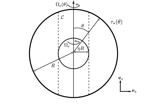
Figure 1: Schematic view of the system: the inner shell of radius $\eta R$ rotates with an angular velocity $\Omega_{c}$ while the outer one of radius $R$ rotates differentially at $\Omega_{s}(\theta)$ by means of a prescribed tangential surface stress $\tau_{*}(\theta)$. The dashed lines correspond to the edges of the tangent cylinder $\mathcal{C}$, circumscribing the inner sphere.

2.1 Description

A fluid of constant kinematic viscosity $\nu$ is enclosed between two spheres (see below). The inner one is rigidly rotating with a constant angular velocity $\Omega_{c}$ while the outer shell supports a prescribed tangential surface-stress $\tau_{*}(\theta)$. $R$ and $\eta R$ are the radii of the outer and inner shells, respectively, and $\theta$ is the colatitude. We sketch out this model in Fig. 1. We consider the driving stress to be sufficiently weak that the rotation period of the system is much shorter than the typical turn-over times associated with the flow in the rotating frame of reference. We thus consider the non-linear terms to be negligible, which we justify a posteriori in Appendix A. The dimensionless equation of vorticity and mass conservation equation in the rotating frame with angular velocity $\Omega_{c}$, and in the context of an “anelastic” flow, read

$$\begin{cases}\begin{aligned} &\frac{\partial}{\partial t}(\boldsymbol{\nabla}\times\rho{\boldsymbol{u}})+\boldsymbol{\nabla}\times({\boldsymbol{e}}_{z}\times\rho{\boldsymbol{u}})=E\boldsymbol{\nabla}\times{\boldsymbol{f}}_{\rm visc}\\ \\ &\boldsymbol{\nabla}\cdot\rho{\boldsymbol{u}}=0\ ,\end{aligned}\end{cases}$$ (1)

where we have used $R$ as the length scale, $(2\Omega_{c})^{-1}$ as the time scale, and $\rho_{c}$, the density at the inner shell, as the density scale. $E$ is the Ekman number defined as

$$E=\frac{\nu}{2\Omega_{c}R^{2}}\ ,$$ (2)

and

$${\boldsymbol{f}}_{\rm visc}=\rho\left(\Delta{\boldsymbol{u}}+\frac{1}{3}\boldsymbol{\nabla}{\rm div}{\boldsymbol{u}}\right)+2(\boldsymbol{\nabla}\rho\cdot\boldsymbol{\nabla}){\boldsymbol{u}}+\boldsymbol{\nabla}\rho\times(\boldsymbol{\nabla}\times{\boldsymbol{u}})-\frac{2}{3}\boldsymbol{\nabla}(\rho{\rm div}{\boldsymbol{u}})\ ,$$ (3)

is the dimensionless viscous force. This expression of the viscous force is meant to represent the case where the envelope is pervaded by some small-scale turbulence with constant diffusive properties as often used in stellar physics (Brandenburg et al., 1996; Käpylä et al., 2012). Centrifugal effects are neglected altogether, and the flows are considered axisymmetric.

This system is then completed by boundary conditions. On the outer shell, we impose a specified stress, which represents the torque resulting from the stellar wind. The simplest dimensionless expression of such a stress, which we take equatorially symmetric, is

$$\tau(\theta)=\sigma_{r\phi}/\rho=-A\sqrt{\frac{3}{4\pi}}\sin\theta,$$

where $[\sigma]$ is the dimensionless stress tensor and $A$ is a positive constant that sets the amplitude of the prescribed (braking) stress. Although the wind imposes a small radial flow at the surface, we shall ignore it in this first approach, and impose a vanishing normal velocity on the outer shell. Finally, we impose no-slip boundary conditions at the inner boundary, as justified by the important viscosity jump at the stellar envelope/core interface. Boundary conditions thus read

$$u_{r}=u_{\theta}=u_{\phi}=0\qquad{\rm at\quad}r=\eta$$ (4a)

$$\left\{\begin{array}[]{l}\displaystyle{u_{r}=r\frac{\partial}{\partial r}\left(\frac{u_{\theta}}{r}\right)=0}\ ,\\ \\ \displaystyle{\frac{\sigma_{r\phi}}{\rho}=r\frac{\partial}{\partial r}\left(\frac{u_{\phi}}{r}\right)=-A\sqrt{\frac{3}{4\pi}}\sin\theta}\end{array}\right.\qquad{\rm at\quad}r=1\ .$$ (4b)

2.2 Numerical method

We use a spectral decomposition and expand the fields in spherical harmonics for the angular part and Chebyshev polynomials for the radial part (see Rieutord & Valdettaro, 1997). We write

$${\boldsymbol{q}}=\rho{\boldsymbol{u}}=\sum^{+\infty}_{l=0}\sum^{+l}_{m=-l}u_{m}^{l}(r)\boldsymbol{R}^{m}_{l}+v_{m}^{l}(r)\boldsymbol{S}^{m}_{l}+w_{m}^{l}(r)\boldsymbol{T}^{m}_{l}\ ,$$ (5)

where

$$\boldsymbol{R}^{m}_{l}=Y^{m}_{l}{\boldsymbol{e}}_{r},\quad\boldsymbol{S}^{m}_{l}=\boldsymbol{\nabla}Y^{m}_{l},\quad\boldsymbol{T}^{m}_{l}=\boldsymbol{\nabla}\times\boldsymbol{R}^{m}_{l}\ ,$$ (6)

with $Y^{m}_{l}$ being the usual normalised scalar spherical harmonic function. Because the ${\boldsymbol{q}}$-flow is divergenceless both in the incompressible and anelastic models, $v_{m}^{l}$ can be expressed as a function of $u_{m}^{l}$ only (Rieutord, 1987). Projecting the vorticity equation (1) on $\boldsymbol{R}^{m}_{l}$ and $\boldsymbol{T}^{m}_{l}$ for an axisymmetric flow ($m=0$), we obtain the following system of equations for the radial parts

$$\begin{cases}\begin{aligned} &\frac{\partial w^{l}}{\partial t}-\left[A_{l-1}^{l}r^{l-1}\frac{\partial}{\partial r}\left(\frac{ru^{l-1}}{r^{l-1}}\right)+A_{l+1}^{l}r^{-l-2}\frac{\partial}{\partial r}(r^{l+3}u^{l+1})\right]=Eh^{l}\ ,\\ &\frac{\partial}{\partial t}\left(\Delta_{l}ru^{l}\right)+B_{l-1}^{l}r^{l-1}\frac{\partial}{\partial r}\left(\frac{w^{l-1}}{r^{l-1}}\right)+B_{l+1}^{l}r^{-l-2}\frac{\partial}{\partial r}(r^{l+2}w^{l+1})=-\frac{E}{r}\left(f^{l}-\frac{\partial rg^{l}}{\partial r}\right)\ ,\\ &v^{l}=\frac{1}{r\Lambda}\frac{\partial r^{2}u^{l}}{\partial r}\ ,\end{aligned}\end{cases}$$ (7)

where $\Lambda=l(l+1)$. $A_{l-1}^{l}$, $A_{l+1}^{l}$, $B_{l-1}^{l}$, and $B_{l+1}^{l}$ are the coupling coefficients defined as

$$A_{l-1}^{l}=A_{l}^{l-1}=\frac{1}{l}\sqrt{\frac{1}{(2l-1)(2l+1)}}\ ,\quad B_{l-1}^{l}=B_{l}^{l-1}=\sqrt{\frac{l(l^{2}-1)}{(2l-1)(2l+1)}}\ .$$ (8)

The viscous force is projected on the spherical harmonics basis as well, namely

$${\boldsymbol{f}}_{\rm visc}=\sum^{+\infty}_{l=0}\sum^{+l}_{m=-l}f_{m}^{l}(r)\boldsymbol{R}^{m}_{l}+g_{m}^{l}(r)\boldsymbol{S}^{m}_{l}+h_{m}^{l}(r)\boldsymbol{T}^{m}_{l}\ ,$$ (9)

where

$$f^{l}=2\frac{\partial\rho}{\partial r}\frac{\Lambda bv^{l}-2bu^{l}}{r}+\frac{\Lambda\rho}{r}z^{l}+\frac{\partial}{\partial r}\left(\frac{4\rho}{3}d^{l}\right)\ ,$$ (10)

$$g^{l}=\frac{1}{r}\frac{\partial}{\partial r}(r\rho z^{l})+\frac{2}{r}\frac{\partial\rho}{\partial r}(bu^{l}-bv^{l})+\frac{4\rho}{3r}d^{l}\ ,$$

$$h^{l}=\rho\Delta_{l}bw^{l}+r\frac{\partial\rho}{\partial r}\frac{\partial}{\partial r}\left(\frac{bw^{l}}{r}\right)\ ,$$

with

$$z^{l}=\frac{1}{r}\frac{\partial rbv^{l}}{\partial r}-\frac{bu^{l}}{r},\quad d^{l}=\frac{1}{r^{2}}\frac{\partial r^{2}bu^{l}}{\partial r}-\frac{\Lambda bv^{l}}{r}\ ,$$ (11)

and where $b(r)=1/\rho(r)$ is the inverse density function.

Finally, the boundary conditions in the rotating frame of reference are projected on the spherical harmonics and read

$$\begin{cases}\begin{aligned} &u^{l}=v^{l}=w^{l}=0\ ,&&{\rm at\ }r=\eta\\ \\ &u^{l}=r\frac{\partial}{\partial r}\left(\frac{bv^{l}}{r}\right)=0\ ,\quad r\frac{\partial}{\partial r}\left(\frac{bw^{l}}{r}\right)=-A\delta_{l1}\ ,\qquad&&{\rm at\ }r=1\ ,\end{aligned}\end{cases}$$ (12)

where $\delta_{ij}$ is the Kronecker symbol.

3 The incompressible flow

In this section, and as a first step, we solve equations (1) for constant density throughout the domain, namely for $\rho(r)=1$, with the boundary conditions (4), and with the initial condition ${\boldsymbol{u}}=\boldsymbol{0}$. Of course, before the steady-state is reached, the flow is in a transient state during which the driving surface stress has not yet been fully communicated to the interior of the fluid. We now briefly analyse this transitional stage so as to estimate the transient time scale.

3.1 The transient phase

As to assess the relevance of the steady-state approximation for geophysical and astrophysical applications, it is important to determine the time scales the flow characteristics are governed by. To do so, we measure the time at which the evolution of the total angular momentum in the rotating frame may be considered to its end. We note that the change in angular momentum of the fluid is due to the difference between the torque exerted on the fluid by the outer boundary condition and the torque that the fluid exerts on the steady inner sphere. Therefore, a stationary state is reached when

$$\Delta\Gamma\equiv\Gamma(1)-\Gamma(\eta)=0\ ,$$ (13)

where $\Gamma(1)$ and $\Gamma(\eta)$ are the torques about the $z$-axis exerted on the outer and inner boundary surface, respectively. The torque about the $z$-axis exerted on a layer located at some radius $r$ can be written

$$\Gamma(r)=\int_{\partial r}\boldsymbol{\sigma}\cdot{\boldsymbol{e}}_{z}dS\ ,$$ (14)

where $\boldsymbol{\sigma}$ is the local stress applied on the sphere of radius $r$. We expand $\boldsymbol{\sigma}$ on the spherical harmonics basis, hence the torque about the $z$-axis reads

$$\Gamma(r)=-\int_{\partial r}r\sin\theta\rho(r)\sum_{l}r^{2}t^{l}\frac{\partial Y_{l}}{\partial\theta}d\Omega\ ,$$ (15)

where

$$t^{l}=r\frac{\partial}{\partial r}\left(\frac{w^{l}}{r}\right)\ .$$ (16)

Using Legendre polynomials recurrence relations, (15) actually reads

$$\Gamma(r)=4\sqrt{\frac{\pi}{3}}r^{3}\rho(r)t^{1}(r)\ .$$ (17)

Applying boundary conditions (12), (13) can finally be written

$$\Delta\Gamma=-4\sqrt{\frac{\pi}{3}}\left(A\rho_{s}+\eta^{3}\frac{\partial w^{1}}{\partial r}\Bigg{|}_{r=\eta}\right)\ ,$$ (18)

where the adimensional surface density $\rho_{s}=\rho(1)=1$ for the considered incompressible model.

We monitor the evolution of the relative difference between the torques $\Delta\Gamma/\Gamma(1)$ for various Ekman numbers and show the result in Fig. 2. It shows that on a time scale $O(E^{-1})$ the stress is completely communicated to the interior flow, and a steady-state is reached.

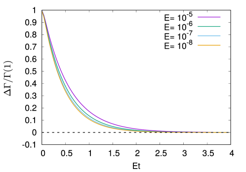
Figure 2: Relative difference between the torque applied on the outer sphere and the torque exerted by the fluid on the stationary inner sphere, as a function of the reduced time $Et$. We find the steady-state to be reached on a $O(E^{-1})$ time scale, that is on a viscous time scale, in the asymptotic regime of small Ekman numbers.

Of course in the astrophysical or geophysical context, it may become necessary to relax the constant rotation of the inner sphere. The torque exerted by the fluid on this boundary can make the inner sphere spin-down. According to the angular momentum theorem

$$\Gamma_{*}(\eta R)=\frac{dL^{\rm core}_{z}}{dt_{*}}=I_{c}\frac{d\Omega_{c}}{dt_{*}}\ ,$$ (19)

where $\Gamma_{*}$ is the dimensional torque, $I_{c}$ is the moment of inertia of the core assumed to be in solid-body rotation, and $L^{\rm core}_{z}$ is its total angular momentum. Starred quantities are dimensional.

The core spin-down then engenders an additional Euler force $\dot{\Omega_{c}}{\boldsymbol{e}}_{z}\times{\boldsymbol{r}}$ since our frame is attached to the core. This force can however be neglected if the timescale associated with the core spin-down is larger than the (viscous) timescale during which the angular momentum is redistributed. In that case, the flow can reach a quasi-steady state. In the present work, for simplicity, we shall use this assumption ($\dot{\Omega_{c}}=0$). Astrophysically, we justify its adoption by the Roche approximation, often used for massive stars, where the whole mass of the star is assumed to be in the core.

Another important time scale is that of the rise of the Stewartson layer. This layer appears as the result of the equatorial singularity of the inner Ekman boundary layer. It is well known that within an equatorial band of latitude $O(E^{1/5})$, the thickness of the Ekman boundary layer is $\delta_{E}=O(E^{2/5})$ (Roberts & Stewartson, 1963). Hence, this singular equatorial viscous boundary layer is expected to be fully developed, and to initiate the development of the Stewartson layer, on the $O(\delta_{E}^{2}/E)=O(E^{-1/5})$ time scale, that is much shorter than the $O(E^{-1})$ viscous time scale. Likewise, the central Stewartson layer of thickness $O(E^{1/3})$ is fully developed on the $O(E^{-1/3})$ time scale, again, much shorter than the viscous time scale. We therefore expect the Stewartson layer to start developing within a few revolutions of the inner shell and to be fully developed on a time scale that is much shorter than the viscous one on which we expect the shear flow inside it to evolve towards the steady-state. We verify this in Fig. 3 showing the amplitude of the stream function $\psi_{h}/\psi_{h,st}$, taken at cylindrical radius $s=\eta$ and $z=1/2$, and normalised by its value at the steady-state, as a function of the reduced time $Et$ for various Ekman numbers.

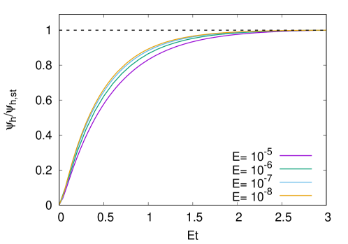
Figure 3: Amplitude of the stream function taken at $s=\eta$ and $z=1/2$ normalised by its value at the steady-state $\psi_{h}/\psi_{h,st}$, as a function of the reduced time $Et$ for various Ekman numbers. We find the Stewartson to appear within a few inner sphere revolutions and to evolve in a viscous time scale.

The analysis of the transient phase preceding the settling of a steady-state thus underlines that the entire meridional flow evolves on a viscous time scale of order $E^{-1}$. In the astrophysical context characterised by extremely small Ekman numbers (typically $E<10^{-10}$), such a scaling implies that a steady-state of the radiative envelope of massive stars is not reached during their lifetime.

3.2 The steady flow

Even if it is not reached during the lifetime of the star, the steady state is worth studying since it owns many simple features and its structure is very similar to that of the transient flow.

It is well known that the linear and stationary vorticity equation of an inviscid incompressible flow verifies Taylor-Proudman theorem (Proudman, 1916; Taylor, 1921), namely

$$({\boldsymbol{e}}_{z}\cdot\boldsymbol{\nabla}){\boldsymbol{u}}=\boldsymbol{0}\ .$$ (20)

For quasi-inviscid interior flows, that is for sufficiently small Ekman numbers, we thus expect a quasi-geostrophic solution for the velocity field. Fig. 4 shows the normalised angular velocity as a function of the cylindrical radial coordinate $s$ for $E=10^{-7}$, $\eta=0.35$, and for various radial distances $r$. Fig. 5 shows a 2D-view of the meridional circulation as well as the differential rotation in the rotating frame for the same model. The resulting flow is characterised by a nested Stewartson shear layer along the tangent cylinder $\mathcal{C}$ where the meridional circulation is essentially concentrated. This narrow shearing region separates two regions of quasi-geostrophic flow: the volume inside and outside $\mathcal{C}$. Inside $\mathcal{C}$, the no-slip conditions on the inner core impose an almost rigid rotation, while outside $\mathcal{C}$ a columnar differential rotation appears as a consequence of the surface stress.

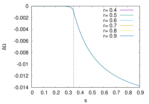
Figure 4: Normalised angular velocity as a function of the cylindrical radial coordinate $s$ for $E=10^{-7}$, $\eta=0.35$, $A=0.01$, and for various $r$.

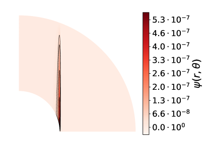
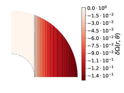
Figure 5: Meridional view of the stream function $\psi$ (left) and of the differential rotation in the rotating frame of reference $\delta\Omega=(\Omega-\Omega_{c})/2\Omega_{c}$ (right) for $E=10^{-7}$, $\eta=0.35$, and $A=0.01$. Three regions can be distinguished: a Stewartson layer on the outer boundary of a tangent cylinder $\mathcal{C}$ of radius $\eta$ separating two regions of weak amplitude circulation. The region inside the cylinder $\mathcal{C}$ corotates with the inner sphere and the region outside $\mathcal{C}$ rotates differentially with a columnar profile.

3.2.1 Flow outside the core tangent cylinder $\mathcal{C}$

We now seek for an analytical solution for both the primary and secondary flows outside $\mathcal{C}$ ($s>\eta$). In the limit of small Ekman numbers, the divergenceless velocity statisfies the Taylor-Proudman theorem, we thus seek a geostrophic solution for both primary and secondary flows outside the tangent cylinder $\mathcal{C}$. Such a solution usually does not satisfy the viscous boundary conditions, however. We thus decompose the dynamical variables as

$${\boldsymbol{u}}=\overline{{\boldsymbol{u}}}+\tilde{{\boldsymbol{u}}}\ ,\qquad{\rm and}\qquad p=\overline{p}+\tilde{p}\ ,$$ (21)

where overlined variable correspond to the interior geostrophic fields, and tilded variables are their boundary layer corrections. Introducing the $O(1)$ stretched boundary layer coordinate $\zeta=(1-r)/\sqrt{E}$, and using the geostrophic equilibrium relation ${\boldsymbol{e}}_{z}\times\overline{{\boldsymbol{u}}}=-\boldsymbol{\nabla}\overline{p}$, the equation of motions, or Ekman boundary layer equation, reads

$${\boldsymbol{e}}_{z}\times\tilde{{\boldsymbol{u}}}=-\frac{\partial\tilde{p}}{\partial\zeta}\boldsymbol{n}+\frac{\partial^{2}\tilde{{\boldsymbol{u}}}}{\partial\zeta^{2}}\ ,$$ (22)

where $\boldsymbol{n}\equiv{\boldsymbol{e}}_{r}$ is the outwardly directed normal vector at the outer shell. Integrating the azimuthal component of (22) from $0$ to $\infty$ yields, at the lowest order,

$$\cos\theta\tilde{Q}=-\frac{\partial\tilde{u}_{\phi}}{\partial\zeta}\Bigg{|}_{\zeta=0}\ {\qquad{\rm with}\qquad}\tilde{Q}=\int_{0}^{\infty}\tilde{u}_{\theta}d\zeta\;.$$ (23)

$\tilde{Q}$ is the outer Ekman layer $\theta$-directed volume flux. Using the boundary condition for the prescribed tangential stress on the outer shell (4), (23) can be rewritten, at the lowest order

$$\cos\theta\tilde{Q}=\sqrt{E}\left[\tau(\theta)-\frac{\partial}{\partial r}\left(\frac{F(s)}{r}\right)\Bigg{|}_{r=1}\right]\ ,$$ (24)

where $F(s)=\overline{u}_{\phi}$ is the geostrophic solution for the azimuthal velocity in the interior. To ensure mass conservation, the divergence of $\tilde{{\boldsymbol{u}}}$ in the boundary layer generates further interior motion by establishing a weak amplitude secondary normal flow $\tilde{u}_{r}$ known as Ekman pumping. This radial velocity can be determined by integrating the mass conservation equation in the outer Ekman boundary layer

$$\tilde{u}_{r} =-\frac{\sqrt{E}}{\sin\theta}\frac{\partial\sin\theta\tilde{Q}}{\partial\theta}$$ (25)

$$=-\frac{E}{\sin\theta}\frac{\partial}{\partial\theta}\frac{\sin\theta}{\cos\theta}\left[\tau(\theta)-\frac{\partial}{\partial r}\left(\frac{F(s)}{r}\right)\Bigg{|}_{r=1}\right]\ .$$

This equation shows that, near the outer shell, and in the Ekman layer, for the boundary condition on the tangential stress to be ensured, there must exist a $O(\sqrt{E})$ tangential flow that, in turn, generates a $O(E)$ circulation in the interior. We now express the geostrophic azimuthal velocity $F(s)$ as a function of the prescribed tangential surface-stress $\tau(\theta)$ driving differential rotation. To do so, we ensure that the no-penetration boundary condition $u_{r}=0$ at $r=1$ is enforced, namely

$$su_{s}+zu_{z}+\tilde{u}_{r}=0\qquad\rm at\;r=1\ ,$$ (26)

where $u_{s}$ and $u_{z}$ are obtained from the azimuthal component of the momentum equation and from the mass conservation equation, respectively. Eq. (26) finally yields a third order ordinary differential equation for $F(s)$

$$-\frac{1-s^{2}}{s^{2}}\frac{\partial}{\partial s}s\left(\nabla^{2}-\frac{1}{s^{2}}\right)F+s\left(\nabla^{2}-\frac{1}{s^{2}}\right)F+\frac{\partial}{\partial s}\left(s^{2}\frac{\partial}{\partial s}\frac{F}{s}\right)+sq\frac{\partial}{\partial s}\frac{F}{s}=-K(1+q(s))\ ,$$ (27)

where $K=A\sqrt{3/4\pi}$. The solutions of (27) can be expressed as an integral functional of the prescribed stress (Friedlander, 1976), that is

$$F(s)=-s\int\frac{ds}{s^{3}\sqrt{1-s^{2}}}\int sds\int\frac{\partial}{\partial s}\left(\frac{-Ks^{2}}{\sqrt{1-s^{2}}}\right)ds\ .$$ (28)

The solution for the geostrophic azimuthal velocity outside the tangent cylinder $\mathcal{C}$, avoiding singularities of the vorticity at $s=1$, and accounting for the no-slip boundary condition at the inner shell finally reads

$$F(s)=-\frac{K}{3}\left(s\ln s-\frac{1}{s}+\alpha(\eta)s\right)\ ,$$ (29)

with

$$\alpha(\eta)=\frac{1}{\eta^{2}}-\ln\eta\ ,$$ (30)

and for which

$$u_{s}=E\left(\Delta-\frac{1}{s^{2}}\right)F(s)=-\frac{2KE}{3s}\ ,\qquad{\rm and}\qquad u_{z}=-\int_{0}^{z}\frac{1}{s}\frac{\partial su_{s}}{\partial s}dz=0\ .$$ (31)

We compare the angular velocity profiles from full numerical solutions to the analytical expression $\delta\Omega=F(s)/s$, for various Ekman numbers and two inner core radii ($\eta=0.1$ and $0.35$) in Fig. 6. The analytical asymptotic solution reproduces rather well our numerical results when the Ekman number is below $10^{-9}$. Our boundary layer analysis also predicts the secondary meridional flow amplitude to be $O(E)$ outside the tangent cylinder $\mathcal{C}$. In Fig. 7 we show the stream function, defined as

$$\frac{\partial\psi}{\partial r}=r\sin\theta u_{\theta},\quad\frac{\partial\psi}{\partial\theta}=-r^{2}\sin\theta u_{r}\ ,$$ (32)

as a function of the cylindrical radial coordinate $s$ for various Ekman numbers. We note that $\psi$ indeed scales as $E$ outside the Stewartson layer, which appears as oscillations of $\psi$ near $s=\eta$. Furthermore, using (31), the stream function associated with the geostrophic solution for the velocity field reads

$$\overline{\psi}(s,z)=-\frac{2KE}{3}z\ ,$$ (33)

implying that streamlines are $z={\rm Cst}$ lines in a meridional plane. Hence, the outer Ekman boundary layer expels fluid in the $s$-direction, towards the Stewartson shear layer. The stream function $\psi$ as well as the corresponding streamlines, from Eq. (33) and from full numerical solutions are represented in Fig. 8, where we have masked the Stewartson layer. We see that the analytical and numerical solutions nicely match. Interestingly, the flow (31) reconnects with the Stewartson layer and partly sources the upwelling flow in this region (see below Sect. 3.2.3).

The foregoing solution shows that the stress-driven spin-down flow is rather different from the spherical Taylor-Couette flow outside the tangent cylinder. For such a flow, the amplitude of the meridional circulation in this region is vanishing exponentially away from the Stewartson layer (Proudman, 1956; Dormy et al., 1998). In our case there is a residual flow, exactly perpendicular to the rotation axis, directed to it, and which scales as the Ekman number.

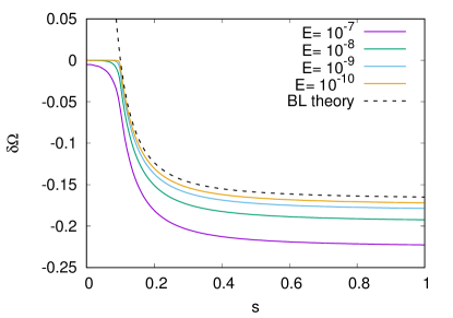
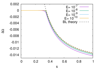
Figure 6: Angular velocity in the rotating frame of reference as a function of the cylindrical radial coordinate $s$ for various Ekman numbers, $r=0.7$, $\eta=0.1$ (left) and $\eta=0.35$ (right), and $A=0.01$. The black dashed line corresponds to the analytical solution $\delta\Omega=F(s)/s$ (see Eq. 29).

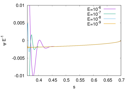
Figure 7: $\psi E^{-1}$ along a meridian at $r=0.7$ as a function of the cylindrical radial coordinate $s$ for various Ekman numbers, $\eta=0.35$, and $A=0.01$. The predicted $O(E)$ scaling of the secondary flow amplitude is verified outside the Stewartson layer, which is located at $s=0.35$.

Figure 8: Meridional view of the stream function and streamlines from full numerical simulations (left), and from the boundary layer analysis (right), for $E=10^{-8}$, $\eta=0.1$, and $A=0.01$. The tangent cylinder $\mathcal{C}$ as well as the adjacent reconnecting layer are masked.

3.2.2 Flow inside the tangent cylinder $\mathcal{C}$

Let us now investigate the geostrophic flow inside the tangent cylinder $\mathcal{C}$. Writing $u_{\phi}=\ell/(r\sin\theta)$ where $\ell$ is the specific angular momentum, the azimutal component of the momentum equation and vorticity equation respectively read (e.g. Goldstein, 1938, 1965; Proudman, 1956; Stewartson, 1966)

$$\begin{cases}\begin{aligned} &\frac{\partial\psi}{\partial r}\cos\theta-\frac{1}{r}\frac{\partial\psi}{\partial\theta}\sin\theta=ED^{2}\ell\\ \\ &-\frac{\partial\ell}{\partial r}\cos\theta+\frac{1}{r}\frac{\partial\ell}{\partial\theta}\sin\theta=ED^{4}\psi\end{aligned}\end{cases}$$ (34)

where

$$D^{2}=\frac{\partial^{2}}{\partial r^{2}}+\frac{\sin\theta}{r^{2}}\frac{\partial}{\partial\theta}\left(\frac{1}{\sin\theta}\frac{\partial}{\partial\theta}\right)\ .$$ (35)

The boundary conditions (4) in terms of streamfunction and specific angular momentum in turn read

$$\psi=\frac{\partial\psi}{\partial r}=\ell=0\qquad{\rm at\quad}r=\eta$$ (36a)

$$\left\{\begin{array}[]{l}\displaystyle{\psi=\frac{\partial^{2}\psi}{\partial r^{2}}-2\frac{\partial\psi}{\partial r}=0}\ ,\\ \\ \displaystyle{\frac{\partial\ell}{\partial r}-2\ell=-K\sin^{2}\theta}\end{array}\right.\qquad{\rm at\quad}r=1\ .$$ (36b)

In the Ekman boundary layers, (34) may be rewritten

$$\begin{cases}\begin{aligned} &\frac{\partial\psi}{\partial r}\cos\theta=E\frac{\partial^{2}\ell}{\partial r^{2}}\\ \\ &-\frac{\partial\ell}{\partial r}\cos\theta=E\frac{\partial^{4}\psi}{\partial r^{4}}\ .\end{aligned}\end{cases}$$ (37)

We integrate the first equation over $r$ to obtain the fourth-order differential equation on $\psi$

$$\frac{\partial^{4}\psi}{\partial r^{4}}=-\frac{\cos^{2}\theta}{E^{2}}(\psi-\overline{\psi})\ ,$$ (38)

where $\overline{\psi}$ is a function of $\theta$ only that can be determined by the boundary conditions (Proudman, 1956). Let us first focus on the outer Ekman layer localised near $r=1$. The solution of (38) satisfying the boundary conditions (36) as well as the condition $\psi(\xi\to\infty)=\overline{\psi}$, where $\xi=(1-r)\sqrt{\cos\theta/2E}$, reads

$$\psi=\overline{\psi}\left(1-e^{-\xi}\cos\xi\right)\ .$$ (39)

From the first equation of (37), we may further write

$$\ell-\overline{\ell}=\overline{\psi}\alpha e^{-\xi}\sin(\xi-\pi/4)\ ,$$ (40)

where $\alpha=\sqrt{\cos\theta/(2E)}\gg 1$ in the asymptotic limit of small Ekman numbers. The boundary condition (36b) then implies

$$\frac{\partial\ell}{\partial r}\Bigg{|}_{r=1}-2\ell(1)=-2\alpha^{2}\overline{\psi}-2\overline{\ell}+2\alpha\overline{\psi}=-K\sin^{2}\theta\ ,$$ (41)

where $\overline{\ell}$ is also a function of $\theta$ only that can be determined by the boundary conditions. Hence, the azimuthal and meridional components of the quasi-geostrophic velocity outside the Ekman and Stewartson shear layers, are not independent and satisfy the outer Ekman jump condition at the lowest order

$$\overline{\psi}=\frac{E}{\cos\theta}(K\sin^{2}\theta-2\overline{\ell})\ .$$ (42)

In a similar way, the study of the inner Ekman layer with boundary conditions (36a) yields

$$\psi=\overline{\psi}\left(1-e^{-\xi^{\prime}}(\cos\xi^{\prime}+\sin\xi^{\prime})\right)\ ,$$ (43)

where $\xi^{\prime}=(r-\eta)\alpha$, and the Ekman jump condition at the inner shell reads

$$\overline{\ell}=-2\overline{\psi}\alpha\ .$$ (44)

Hence (44) implies $\overline{\psi}=O(\overline{\ell}\sqrt{E})$ and thus (42) implies $\overline{\psi}=O(E)$ and $\overline{\ell}=O(\sqrt{E})$. We may therefore rewrite (42) as

$$\overline{\psi}=\frac{E}{\cos\theta}K\sin^{2}\theta+O(E^{3/2})\ .$$ (45)

Finally, the geostrophic solution for the velocity inside the tangent cylinder $\mathcal{C}$ ($s<\eta$) reads, at the lowest order,

$$\overline{\psi}(s)=\frac{EKs^{2}}{\sqrt{1-s^{2}}}\qquad{\rm and}\qquad\delta\Omega=\frac{\overline{\ell}(s)}{s^{2}}=-\frac{\sqrt{2E}K}{\sqrt{1-s^{2}}}\left(1-\frac{s^{2}}{\eta^{2}}\right)^{1/4}\ ,$$ (46)

and the meridional components of the geostrophic velocity at the lowest order

$$u_{s}=\frac{1}{s}\frac{\partial\overline{\psi}}{\partial z}=0\qquad{\rm and}\qquad u_{z}=-\frac{1}{s}\frac{\partial\overline{\psi}}{\partial s}=-\frac{EK}{\sqrt{1-s^{2}}}\left(1+\frac{1}{1-s^{2}}\right)\ .$$ (47)

We compare these analytical $z$-directed velocity and angular velocity profiles with full numerical solutions in Fig. 9, for various $E$. We find our analytical expression to be in good agreement with the numerical solutions. Remarkably, the meridional flow inside the tangent cylinder is parallel to the rotation axis and directed towards the inner core, which is quite different from the outer-${\cal C}$ meridional flow. Once inside the inner Ekman layer, the flow heads towards the equator where the Ekman layer thickens and eventually changes scale at the equatorial singularity (e.g., Roberts & Stewartson, 1963; Stewartson, 1966; Hollerbach, 1994; Dormy et al., 1998; Marcotte et al., 2016). The fluid then returns to the outer Ekman layer following the Stewartson layer. Fig. 10 shows the meridional view of two arbitrarily selected streamlines, one inside and one outside the tangent cylinder $\mathcal{C}$. It illustrates the different shape of the secondary flow in the two regions, as well as the reconnecting shear layer redirecting the $s$-direction flow outside $\mathcal{C}$ to the Stewartson layer where it flows parallel to the rotation axis towards the outer boundary.

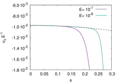
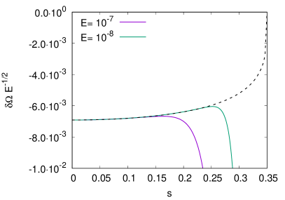
Figure 9: $z$-directed velocity $u_{z}E^{-1}$ (left) and angular velocity in the rotating frame of reference (right) inside the tangent cylinder $\mathcal{C}$ as a function of the cylindrical radial coordinate $s$, for $E=10^{-7}$ and $E=10^{-8}$, $r=0.7$, and $\eta=0.35$. The black dashed line corresponds to the analytical geostrophic solutions (46) and (47).

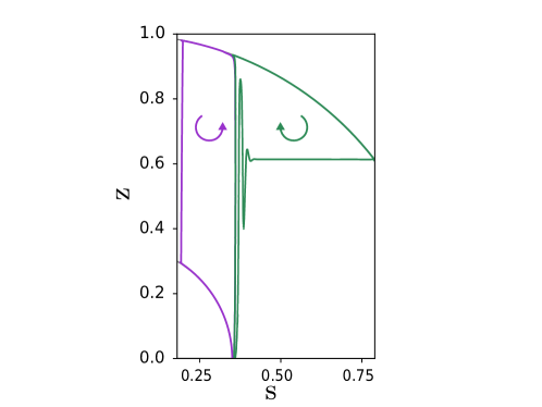
Figure 10: Meridional view of two arbitrarily selected streamlines, inside and outside the tangent cylinder $\mathcal{C}$. The arrows indicate the direction of propagation of the fluid along the streamlines.

3.2.3 Flow in the nested Stewartson shear layer

In Fig. 7 and Fig. 9 we see that the meridional flow strongly deviates from the analytical solution as one nears the Stewartson layer. From the numerical solution, the amplitude of the meridional circulation turns out to be much stronger in this layer than outside it. This is obvious if we compute the total meridional kinetic energy of the secondary flow

$$E_{k,\rm tot}=\int V_{m}^{2}dV\ ,$$ (48)

where $V_{m}^{2}=u_{r}^{2}+u_{\theta}^{2}$. In Fig. 11a we show $E_{k,\rm tot}$ as a function of the Ekman number. We find $E_{k,\rm tot}$ to scale as $E$ in the asymptotic regime $E\to 0$, whereas the contribution of the flows outside the Stewartson layer remains $O(E^{2})$. Hence, the Stewartson layer deserves some investigation.

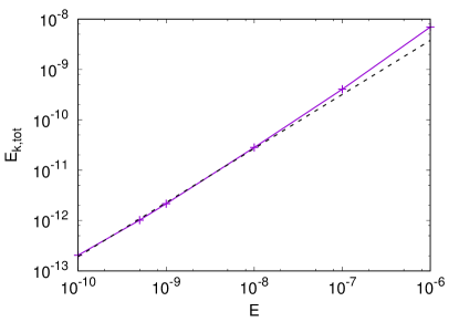
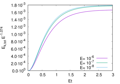
Figure 11: Left: Total meridional kinetic energy of the stationary flow as a function of the Ekman number, for $A=0.01$ and $\eta=0.1$. The black dashed line corresponds to the fit in the asymptotic regime ($E\lesssim 10^{-9}$) and yields $E_{k,\rm tot}\propto E^{1.074}$. Right: $E_{k,\rm tot}E^{-1.074}$ as a function of the reduced time $Et$ for various Ekman numbers, $A=0.01$, and $\eta=0.35$.

We first recall that in the Taylor-Couette flow the Stewartson layer is a nested shear layer that can be split into three layers of width $E^{2/7}$, $E^{1/3}$ and $E^{1/4}$ (Stewartson, 1966). The $E^{1/3}$-layer is the central layer, while the $E^{2/7}$-layer is on the inner side and the $E^{1/4}$ on the outer side. We now wish to find out if these three nested layers are present in our models. Let us start by noticing that, according to (25), the Ekman pumping may be written

$$\tilde{u}_{r}=-\sqrt{E}\left[\boldsymbol{\nabla}\times(\tilde{Q}{\boldsymbol{e}}_{\phi})\right]\cdot{\boldsymbol{e}}_{r}\ .$$ (49)

Hence, introducing the adimensional cartesian stretched coordinate of order $O(1)$ in a shear layer parallel to the rotation axis, outside the tangent cylinder, and of thickness $O(E^{\gamma})$, $\xi=E^{-\gamma}(s-\eta)$, we get

$$\tilde{u}_{r}=O\left[\left(E\boldsymbol{\nabla}\times\left(E^{-\gamma}\frac{\partial F}{\partial\xi}{\boldsymbol{e}}_{\phi}\right)\right)\right]\cdot{\boldsymbol{e}}_{r}=O(E^{1-2\gamma})\ ,$$ (50)

where $F=\overline{u}_{\phi}$. We conclude that, in such layers, the radial velocity resulting from the Ekman pumping/suction is of order $O(E^{1-2\gamma})$. The mass conservation equation, in turn, reads

$$E^{-\gamma}\frac{\partial u_{s}}{\partial\xi}+\frac{\partial u_{z}}{\partial z}=0\ ,$$ (51)

implying that in such a shear layer $u_{z}=O(E^{-\gamma}u_{s})$, that is $u_{z}\gg u_{s}$ in the asymptotic regime of small Ekman numbers.

Simple manipulations of the momentum and vorticity equations allow us to eliminate the velocity $\boldsymbol{u}$ and lead to the following sixth order partial differential equation for the pressure (Greenspan, 1968)

$$\frac{\partial^{2}p}{\partial z^{2}}+E^{2-6\gamma}\frac{\partial^{6}p}{\partial\xi^{6}}=0\ ,$$ (52)

representing a balance between Coriolis and viscous forces. The equality of these two terms thus requires $\gamma=1/3$, and indicates a shear layer of thickness $O(E^{1/3})$ as expected. Hence, in this central ageostrophic layer, we expect

$$u_{s}=O(E^{2/3})\ ,\qquad{\rm and}\qquad u_{z}=O(E^{1/3})\ .$$ (53)

Let us now recall that the quasi-geostrophic $E^{1/4}$ layer is associated with the equilibrium between the Ekman pumping flow, and the internal friction of the $O(1)$ azimuthal flow (e.g., Stewartson, 1966; Barcilon, 1968). This equilibrium is, in fact, exactly that which is in place in the entire region outside the tangent cylinder $\mathcal{C}$, and the $E^{1/4}$-layer is therefore not needed. Indeed, the azimuthal component of the momentum equation in the boundary layer of thickness $O(E^{\gamma})$ reads

$$u_{s}=E^{1-2\gamma}\frac{\partial^{2}u_{\phi}}{\partial\xi^{2}}\ ,$$ (54)

that is $u_{s}=O(E^{1-2\gamma})$ if we assume $u_{\phi}=O(1)$. In addition, (51) further implies $u_{z}=O(E^{1-3\gamma})$. However, the Ekman pumping still demands $u_{z}=O(E^{1-2\gamma})$ (see Eq. 49). Hence, $\gamma=0$ and the equilibrium between the Ekman pumping flow and the internal friction of the $O(1)$ azimuthal flow does indeed occur in a $O(1)$ “layer” that is the entire $s>\eta$ region. Note that if we had considered no-slip boundary conditions at the outer shell, that is the case of a spherical Taylor-Couette flow, the $z$-directed velocity resulting from the Ekman pumping would be of order $O(\sqrt{E}\boldsymbol{\nabla}\times\overline{u}_{\phi}{\boldsymbol{e}}_{\phi})=O(E^{1/2-\gamma})$. The matching of the $u_{z}$-flux and the Ekman pumping implies that $1/2-\gamma=1-3\gamma$, and thus $\gamma=1/4$ as expected.

Let us finally consider the case of a quasi-geostrophic $z$-directed free shear layer of thickness $O(E^{\gamma^{\prime}})$ located inside the tangent cylinder $\mathcal{C}$ and near $s=\eta$. It follows that in such a region, $\ell$ is a function of $s$ only. Note that in the case of a spherical Taylor-Couette flow, $\gamma^{\prime}=2/7$ and $u_{\phi}(s=\eta)=O(E^{1/28})$ (e.g. Stewartson, 1966; Marcotte et al., 2016). In this region, the azimuthal component of the moment equation (34a) integrated over $z$ reads

$$\psi=Ez\frac{\partial^{2}\ell}{\partial s^{2}}+f(s)\ ,$$ (55)

where $f(s)$ is determined by applying the inner Ekman layer jump condition (44) at $z=0$ and $s-\eta\ll 1$ (Stewartson, 1966), yielding

$$f(s)\simeq-\sqrt{\frac{E}{2}}\left[2\left(1-\frac{s}{\eta}\right)\right]^{-1/4}\ell\ .$$ (56)

In addition, at $z=\sqrt{1-\eta^{2}}$, that is at $r=1$ and $s=\eta$, (42) reads

$$\psi=\frac{EK\eta^{2}}{\sqrt{1-\eta^{2}}}\ ,$$ (57)

and (55) finally becomes

$$E^{1-2\gamma^{\prime}}\frac{\sqrt{1-\eta^{2}}}{\eta^{4}}\frac{d^{2}\ell}{dx^{2}}-E^{1/2-\gamma^{\prime}/4}(2x)^{-1/4}\ell=\frac{EK\eta^{2}}{\sqrt{1-\eta}}\ ,$$ (58)

where we have introduced the stretched $O(1)$ shear layer coordinate $x=(1-s/\eta)/E^{\gamma^{\prime}}$. At this point, it is interesting to determine the correct balancing in (58). We note that the only balance implying the existence of an asymptotically narrow shear layer is that of the first two terms, the third one being of higher order. This balance enforces $\gamma^{\prime}=2/7$, that is a standard inner Stewartson shear layer of thickness $O(E^{2/7})$. Hence, the second order ordinary differential equation for the specific angular momentum at the lowest order and in the $E^{2/7}$ shear layer reads

$$\frac{d^{2}\ell}{dx^{2}}-\beta x^{-1/4}\ell=0\ ,$$ (59)

where

$$\beta=\frac{\eta^{2}}{2^{3/4}\sqrt{1-\eta^{2}}}\ .$$ (60)

This equation can be transformed into a Bessel equation, and the solution asymptotically matching the solution (46), that is decaying to zero as $x\to+\infty$, reads (see also Stewartson, 1966; Moore & Saffman, 1968; Marcotte et al., 2016)

$$\ell(x)=\ell(0)C\sqrt{x}K_{4/7}\left(\frac{8}{7}\sqrt{\beta}x^{7/8}\right)\ ,$$ (61)

where $K_{\nu}(z)$ is the modified Bessel function of second kind and $C$ is a constant to be determined. We note that

$$\lim_{x\to 0}\sqrt{x}K_{4/7}\left(\frac{8}{7}\sqrt{\beta}x^{7/8}\right)=\frac{\Gamma\left(4/7\right)}{2\beta^{2/7}}\left(\frac{7}{4}\right)^{4/7}+O(x)$$

and thus, at the lowest order

$$C=\frac{2\beta^{2/7}}{\Gamma\left(4/7\right)}\left(\frac{4}{7}\right)^{4/7}\ .$$ (62)

Finally, $d\ell/ds$ is rendered continuous across $s=\eta$ in the two quasi-geostrophic regions, that is

$$\frac{d\ell}{ds}\Bigg{|}_{s=\eta^{-}}=\frac{d\ell}{ds}\Bigg{|}_{s=\eta^{+}}\ ,$$ (63)

which yields the specific angular momentum at $s=\eta$

$$\ell(0)=-\frac{K\eta^{2}E^{2/7}}{3\beta^{4/7}}\left(\frac{2}{\eta^{2}}+1\right)\left(\frac{7}{4}\right)^{1/7}\frac{\Gamma(4/7)}{\Gamma(3/7)}=O(E^{2/7})\ .$$ (64)

We verify the shear layer thickness as well as the analytical azimuthal velocity profile (61) comparing it with full numerical solutions in Fig. 12a. The lowest order solution for the azimuthal velocity in the entire $s\leq\eta$ domain is shown in Fig. 12b. Finally, using (55), the corresponding stream function reads

$$\psi(x)=-\frac{2K\eta^{2}E^{5/7}}{3\beta^{2/7}\Gamma(3/7)}\left(\frac{2}{\eta^{2}}+1\right)\left(\frac{4}{7}\right)^{3/7}x^{1/4}K_{4/7}\left(\frac{8}{7}\sqrt{\beta}x^{7/8}\right)\left[\frac{\beta z}{\eta^{2}}-\frac{1}{2^{3/4}}\right]\ ,$$ (65)

and thus

$$u_{s} =-\frac{B_{s}E^{5/7}}{1-xE^{2/7}}x^{1/4}K_{4/7}\left(\frac{8}{7}\sqrt{\beta}x^{7/8}\right)$$ (66)

$$u_{z} =\frac{B_{z}E^{3/7}}{x^{3/4}(1-xE^{2/7})}\left(K_{4/7}\left(\frac{8}{7}\sqrt{\beta}x^{7/8}\right)+4\sqrt{\beta}x^{7/8}K_{3/7}\left(\frac{8}{7}\sqrt{\beta}x^{7/8}\right)\right)\ ,$$

in the $E^{2/7}$-layer, where

$$B_{s}=\frac{2K\beta^{5/7}}{3\eta\Gamma(3/7)}\left(\frac{2}{\eta^{2}}+1\right)\left(\frac{4}{7}\right)^{3/7}$$ (67)

and

$$B_{z}=\frac{K\left(2+\eta^{2}\right)}{6\eta^{2}\beta^{2/7}\Gamma(3/7)}\left(\frac{4}{7}\right)^{3/7}\left(\frac{\beta z}{\eta^{2}}-\frac{1}{2^{3/4}}\right)\ .$$ (68)

We verify the validity of the solution (65) in the $E^{2/7}$-layer away from the $E^{1/3}$-layer in Fig. 13. We note that $\psi$ and its derivatives remain discontinuous across $s=\eta$, hence, contrary to the differential rotation (61), the solution (65) is not valid in the close vicinity of $s=\eta$, and it is the ageostrophic $E^{1/3}$-layer that smoothes them out. Furthermore, since $3/7>1/3$, the $z$-component of the velocity is expected to be maximum in the $E^{1/3}$ layer.

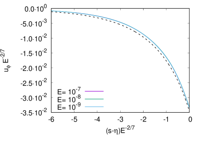
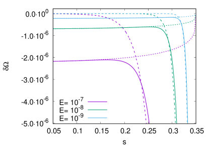
Figure 12: Left: $u_{\phi}E^{-2/7}$ as a function of the stretched cylindrical radial coordinate $(s-\eta)E^{-2/7}$ for various Ekman numbers, $\eta=0.35$, $z=0.7$, and $A=0.01$. The black dashed line corresponds to the analytical geostrophic solution (61). Right: Angular velocity in the rotating frame of reference as a function of the cylindrical radial coordinate $s$. The dashed lines correspond to the analytical solutions (46) and (61).

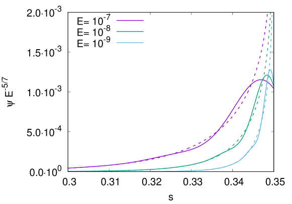
Figure 13: $\psi E^{-5/7}$ as a function of the cylindrical radial coordinate $s$ for various Ekman numbers, $\eta=0.35$, $z=0.7$, and $A=0.01$. The dashed lines correspond to the analytical geostrophic solutions (65).

We further verify the scalings for the thickness of the two Stewartson shear layers, as well as that of the amplitude of their associated $s$- and $z$-directed velocity numerically, in Fig. 14 and in Fig. 15. Though the amplitude of the $z$-directed velocity is, as expected, maximum in the central Stewartson layer, we find a slight discrepancy with the expected power laws for the velocity near $s=\eta$. This discrepancy is, in fact, not surprising as these two Stewartson shear layers are nested. The velocity in the region where the two coexist, that is the $E^{1/3}$-layer, is thus expected to follow both (53) and (66). In practice, we measure

$$u_{s}\simeq O(E^{0.7})\ ,\qquad{\rm and}\qquad u_{z}\simeq O(E^{0.37})\ ,$$ (69)

which lies in-between the velocity scalings in the two layers. For simplicity’s sake, we may consider the amplitude scaling of meridional velocity in the $E^{1/3}$-layer to be that of Eq. 53, that is $u_{s}=O(E^{2/3})$ and $u_{z}=O(E^{1/3})$.

Ultimately, we find our results to be consistent with the scaling of the kinetic energy $E_{k,\rm tot}\propto E$, which suggest that the main contribution comes from a $E^{1/3}$-velocity field spread over a free shear layer of width $E^{1/3}$. This $E^{1/3}$ amplitude scaling of the velocity field in the Stewartson layer is actually verified throughout the transient, as can be seen in Fig. 11b. This implies that despite a steady-state seemingly not being reached in the lifetime of massive stars, the time relevant for the advective transport of angular momentum and of chemicals within their radiative envelope scales as $E^{-2/3}$, since the the whole meridional velocity grows on a viscous time scale (e.g. Fig. 3).

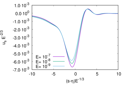
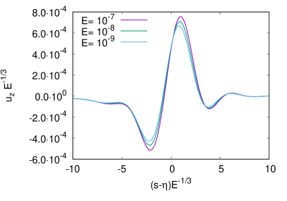
Figure 14: $u_{s}E^{-2/3}$ (left) and $u_{z}E^{-1/3}$ (right) as a function of the stretched cylindrical radial coordinate $(s-\eta)E^{-1/3}$ for various Ekman numbers, $\eta=0.35$, $z=0.7$, and $A=0.01$.

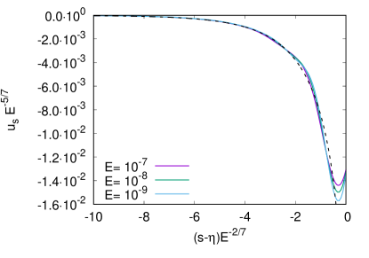
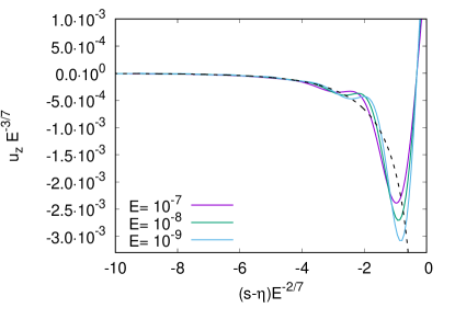
Figure 15: $u_{s}E^{-5/7}$ (left) and $u_{z}E^{-3/7}$ (right) as a function of the stretched cylindrical radial coordinate $(s-\eta)E^{-2/7}$ for various Ekman numbers, $\eta=0.35$, $z=0.7$, and $A=0.01$. The black dashed lines correspond to the solution (66).

3.3 Conclusions

The picture which results from the foregoing discussion is rather neat. The spherical shell is split into three domains:

1. The domain outside the tangent cylinder ${\cal C}$, $s>\eta$ where at first order, and outside any layer,

   $$u_{s}=-\frac{2KE}{3s},\quad u_{\phi}=-\frac{K}{3}\left(s\ln s/\eta-\frac{1}{s}+\frac{s}{\eta^{2}}\right),\quad u_{z}=0$$

   Thus for a braking torque, $u_{\phi}<0$ and $u_{s}<0$ so that there is a weak radial flow towards the Stewartson layer.

2. The domain inside the tangent cylinder, $s<\eta$ where we find that

   $$u_{s}=0,\quad u_{\phi}=-\frac{\sqrt{2E}Ks}{\sqrt{1-s^{2}}}\left(1-\frac{s^{2}}{\eta^{2}}\right)^{1/4},\quad u_{z}=-\frac{EK}{\sqrt{1-s^{2}}}\left(1+\frac{1}{1-s^{2}}\right)$$

3. In between, the Stewarston layer is composed of two nested shear layers of thickness $O(E^{2/7})$ and $O(E^{1/3})$, and is dominated by a flow parallel to the rotation axis and directed towards the outer shell. In the $E^{2/7}$-layer,

   $$u_{s}\sim E^{5/7},\qquad u_{\phi}\sim E^{2/7},\qquad u_{z}\sim E^{3/7}$$

   and in the $E^{1/3}$-layer,

   $$u_{s}\sim E^{2/3},\qquad u_{\phi}\sim E^{1/3},\qquad u_{z}\sim E^{1/3}$$

   Hence the meridional circulation is completely dominated by the shear flow of the $E^{1/3}$ Stewartson layer.

4 The role of thermal stratification

4.1 Description

Stable stratification introduces a restoring buoyancy force that acts to inhibit vertical motions and may partially or entirely eliminate the control of the flow exercised by the Ekman layers. Indeed, the tendency for viscous layers to generate secondary circulation is counteracted by the stable stratification. Thus, we may wonder to what extent the flow inside the stably stratified radiative envelope of a massive star losing angular momentum can remain properly modelled with a geostrophic solution. To investigate this question we introduce a radially stable stratification and use the Boussinesq approximation. We still neglect the centrifugal acceleration. The linearised and dimensionless vorticity, mass conservation, and heat equations read

$$\begin{cases}\begin{aligned} &\frac{\partial}{\partial t}\left(\boldsymbol{\nabla}\times{\boldsymbol{u}}\right)+\boldsymbol{\nabla}\times({\boldsymbol{e}}_{z}\times{\boldsymbol{u}}-\delta T{\boldsymbol{r}})=E\Delta\boldsymbol{\nabla}\times{\boldsymbol{u}}\ ,\\ \\ &\boldsymbol{\nabla}\cdot{\boldsymbol{u}}=0\ ,\\ \\ &\frac{\partial\delta T}{\partial t}+\Pran Sru_{r}=E\Delta\delta T\ ,\end{aligned}\end{cases}$$ (70)

where we have used $\Delta T(2\Omega_{c})^{2}/{\cal N}^{2}$ as the temperature scale. $\Delta T$ is the temperature difference between outer and inner shells, and $\mathcal{N}$ is the the Brunt-Väisälä frequency defined as

$${\cal N}^{2}=\frac{\alpha g\Delta T}{R}\ ,$$ (71)

where $\alpha$ is the coefficient of thermal expansion and $\boldsymbol{g}=-g{\boldsymbol{r}}$ is the gravitational field. We have assumed the equilibrium temperature gradient to be produced by a uniform distribution of heat source (Chandrasekhar, 1961), which implies that $\boldsymbol{\nabla}T_{\rm eq,*}=(\Delta T/R^{2})r{\boldsymbol{e}}_{r}$. $\delta T$ is the temperature perturbation from such thermal equilibrium, and $\Pran=\nu/\kappa_{T}$ is the Prandtl number, which only enters the equations of motion combined with $S={\cal N}^{2}/(2\Omega_{c})^{2}$, as actually noted by Barcilon & Pedlosky (1967). $\kappa_{T}$ is the heat diffusivity that we have assumed to be constant. In what follows, we use the dimensionless parameter introduced by Garaud (2002), namely

$$\lambda=\Pran\frac{{\cal N}^{2}}{(2\Omega_{c})^{2}}\ ,$$ (72)

as the parameter characterising the effective strength of thermal stratification.

We complete these equations with the boundary conditions (4) for the velocity field, and we impose $\delta T=0$ at the boundaries. The initial conditions are ${\boldsymbol{u}}=\boldsymbol{0}$, and $\delta T=0$. Projecting (70) on spherical harmonics yields the following system of equations for radial parts

$$\begin{cases}\begin{aligned} &\frac{\partial w^{l}}{\partial t}-\left[A_{l-1}^{l}r^{l-1}\frac{\partial}{\partial r}\left(\frac{ru^{l-1}}{r^{l-1}}\right)+A_{l+1}^{l}r^{-l-2}\frac{\partial}{\partial r}(r^{l+3}u^{l+1})\right]=E\Delta_{l}w^{l}\ ,\\ &\frac{\partial}{\partial t}\left(\Delta_{l}ru^{l}\right)+B_{l-1}^{l}r^{l-1}\frac{\partial}{\partial r}\left(\frac{w^{l-1}}{r^{l-1}}\right)+\frac{B_{l+1}^{l}}{r^{l+2}}\frac{\partial}{\partial r}(r^{l+2}w^{l+1})+\Lambda T^{l}=E\Delta_{l}\Delta_{l}ru^{l}\ ,\\ \\ &\frac{\partial T^{l}}{\partial t}+\lambda ru^{l}=E\Delta_{l}T^{l}\ ,\end{aligned}\end{cases}$$ (73)

where

$$\delta T(r,\theta)=\sum_{l=0}^{+\infty}T^{l}(r)Y_{l}(\theta)\ .$$ (74)

Fig. 16 shows the differential rotation in the rotating frame of reference and the meridional circulation for $E=10^{-7}$ and various $\lambda$ once the steady-state is settled. We see that the flow departs from the quasi-geostrophic equilibrium as $\lambda$ increases. At high $\lambda$ the angular velocity profile thus becomes shellular, namely it only depends on the radial distance.

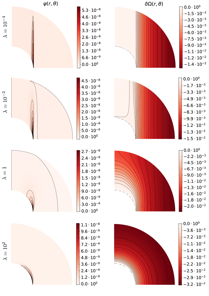
Figure 16: Meridional view of the stream function $\psi$ (left) and of the differential rotation in the rotating frame of reference $\delta\Omega=(\Omega-\Omega_{c})/(2\Omega_{c}$) (right) for $E=10^{-7}$, $\eta=0.35$, $A=0.01$, and various $\lambda$.

4.2 Horizontal boundary layers

In the case of a thermally homogeneous fluid, we have seen that horizontal boundary layers, and specifically Ekman layers play a crucial role on the interior dynamics of the flow. Hence, one may wonder how such layers impact the interior flow in a thermally stratified fluid. We first consider the condition of existence of such horizontal boundary layers and determine their thickness scaling with the relevant adimensional parameters.

Inside boundary layers, horizontal length scales are much larger than the transverse one. Radial derivatives are therefore expected to prevail. We thus write the simplified equations, assuming $\partial_{r}\gg\partial_{\theta}$ in horizontal boundary layers

$$\begin{cases}\begin{aligned} -u_{\phi}\sin\theta&\simeq-\frac{\partial p}{\partial r}+\delta Tr+E\frac{\partial^{2}u_{r}}{\partial r^{2}}\\ -u_{\phi}\cos\theta&\simeq-\frac{1}{r}\frac{\partial p}{\partial\theta}+E\frac{\partial^{2}u_{\theta}}{\partial r^{2}}\\ u_{\theta}\cos\theta+u_{r}\sin\theta&\simeq E\frac{\partial^{2}u_{\phi}}{\partial r^{2}}\\ \frac{\partial u_{r}}{\partial r}+\frac{1}{r}\frac{\partial u_{\theta}}{\partial\theta}&\simeq 0\\ ru_{r}&\simeq\frac{E}{\lambda}\frac{\partial^{2}\delta T}{\partial r^{2}}\ .\end{aligned}\end{cases}$$ (75)

Combining these equations, only keeping the highest order derivatives for each coefficient ($E^{2}$, $\lambda$ and 1) yields the general horizontal boundary layer equation

$$E^{2}r\frac{\partial^{6}u_{\theta}}{\partial r^{6}}+\lambda\frac{\partial^{2}u_{\theta}}{\partial\theta^{2}}-r\cos^{2}\theta\frac{\partial^{2}u_{\theta}}{\partial r^{2}}\simeq 0\ .$$ (76)

Introducing the $O(1)$ stretched radial coordinate $\zeta=(1-r)/\sqrt{E}$, (76) can be re-written, in the outer boundary layer and in the asymptotic regime of small Ekman numbers,

$$\frac{1}{E}\frac{\partial^{6}u_{\theta}}{\partial\zeta^{6}}+\lambda\frac{\partial^{2}u_{\theta}}{\partial\theta^{2}}-\frac{1}{E}\cos^{2}\theta\frac{\partial^{2}u_{\theta}}{\partial\zeta^{2}}\simeq 0\ .$$ (77)

We see that if $\lambda\ll 1/E$, we get the actual Ekman layer where the Coriolis force is balanced by the viscous shear. As remarked by Barcilon & Pedlosky (1967), we note that, whenever Ekman layers are present, their structure is independent of the stratification strength because the forces in balance in such layers essentially involve horizontal motions. Similarly, if $\lambda\gg 1$, introducing the stretched radial coordinate $\gamma=(1-r)\sqrt{\lambda}$, (76) can be re-written, in the outer boundary layer,

$$E^{2}\lambda^{2}\frac{\partial^{6}u_{\theta}}{\partial\gamma^{6}}+\frac{\partial^{2}u_{\theta}}{\partial\theta^{2}}-\cos^{2}\theta\frac{\partial^{2}u_{\theta}}{\partial\gamma^{2}}\simeq 0\ .$$ (78)

Hence, if $1\ll\lambda^{2}\ll 1/E^{2}$, the viscous term drops out and buoyancy balances the Coriolis force. This is typical of a thermal boundary layer of width $\delta_{\lambda}=O(1/\sqrt{\lambda})$. We note that in the parameter regime $\lambda\ll 1$, only Ekman layers are present at the boundaries, while in the regime $1\ll\lambda\ll 1/E$ both thermal and Ekman boundary layers coexist. In this latter case thermal boundary layers are always much thicker than Ekman layers.

4.3 Massive stars interior flows

From the foregoing discussion, it turns out that the dynamics of the flows may be quite different whether $\lambda\gg 1$ or $\lambda\ll 1$. Let us now place the case of rapidly rotating massive stars.

We note that, in the envelope of massive stars, the radiative viscosity and radiative heat diffusion largely dominate diffusion of collisional origin (Espinosa Lara & Rieutord, 2013). These two quantities read

$$\nu_{\rm rad}=\frac{4aT^{4}}{15c\kappa_{R}}\ ,\quad\ \kappa_{\rm rad}=\frac{4acT^{3}}{3\kappa_{R}c_{p}}\ ,$$ (79)

where $T$ is the temperature, $\kappa_{R}$ is the Rosseland mean opacity, $a=4\sigma/c$ is the radiation density constant with $\sigma$ the Stefan-Boltzmann constant, $c$ the speed of light and $c_{p}$ is the specific heat capacity at constant pressure. In such a radiation-dominated system, the radiative Prandtl number reads

$$\Pran_{\rm rad}=\frac{3}{10}\frac{c_{s}^{2}}{c^{2}}\ ,$$ (80)

where $c_{s}$ is the adiabatic sound speed, showing that, naturally, $\Pran_{\rm rad}\ll 1$.

However, the differential rotation of the radiative envelope is expected to drive some small-scale turbulence. Zahn (1992) proposes that the turbulent vertical kinematic viscosity associated with marginal shear stability reads as

$$\nu_{t}=\frac{\Ri_{c}\kappa_{T}}{3}\left(\frac{s}{{\cal N}}\frac{d\Omega}{ds}\right)^{2}\ ,$$ (81)

where $Ri_{c}\simeq 1/4$ is the critical Richardson number. In Fig. 17, we plot the radiative and turbulent Prandtl numbers radial profiles at the equator of a 15 solar mass star as given by a 2D-ESTER model (Rieutord et al., 2016) for various rotation rates defined as the ratio $\omega$ between the equatorial angular velocity and the equatorial Keplerian angular velocity. The associated radial profiles of $\lambda$ are also shown. Although the turbulent Prandtl number is a few orders of magnitude larger than the radiative one in fast rotating stars, turbulent $\lambda$ is just one order of magnitude larger.

We find that the turbulent $\lambda$-parameter is roughly independant of $\omega$, and never exceeds $10^{-3}$ in the considered models. The radiative $\lambda$-parameter, on the other hand, increases for decreasing $\omega$ to the point it may locally exceed $10^{-4}$ when $\omega\lesssim 0.1$. As massive stars are often considered to be fast rotators, we conclude that the thermal stratification regime of their radiative envelope corresponds to $\lambda\ll 1$.

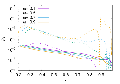
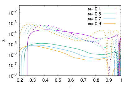
Figure 17: $\Pran$ and $\lambda$ radial profiles at the equator measured from ESTER 2D stellar models of a 15 $M_{\odot}$ star, for various angular velocity ratios $\omega$. The radiative Prandtl number $\Pran_{\rm rad}$ and the corresponding $\lambda$-parameter are represented in full lines, and their turbulent counterparts are represented in dashed lines.

4.4 Asymptotically weak thermal stratification regime

We now study the case of weak temperature stratification, relevant to the radiative envelope of rotating massive stars. In other context the $\lambda\ll 1$ regime may also be reached if the Brunt-Väisälä frequency is just small. We have seen that in this regime, only Ekman layers characterised by an $O(E)$ radial velocity at their edge, are present at the boundaries. We thus assume $\lambda\ll 1$ for the weak stratification, but also suppose that $E\ll\lambda$ as expected in stars.

4.4.1 The steady flow

We first focus on the steady flow. The radial component of the steady momentum equation reads

$$-u_{\phi}\sin\theta=-\frac{\partial p}{\partial r}+\delta Tr+E\left[\Delta u_{r}-\frac{2}{r^{2}}\left(u_{r}+\frac{1}{\sin\theta}\frac{\partial\sin\theta u_{\theta}}{\partial\theta}\right)\right]\ ,$$ (82)

where differential rotation is driven by the $O(1)$ surface stress, that is $u_{\phi}=O(1)$. In the asymptotic regime of small Ekman number, the temperature deviation from equilibrium is therefore, at most, $O(1)$. If that is the case, namely if $\delta T=O(1)$, the heat equation (70) implies that the interior radial velocity $u_{r}$ is $O(E/\lambda)$, namely larger than the $O(E)$ Ekman pumping (25), in the considered stratification regime. Because of the boundary conditions imposed by Ekman layers, an $O(E/\lambda)$ radial velocity must vanish at $r=\eta$ and $r=1$. Furthermore, the radial component of the vorticity equation reads

$$\frac{\partial u_{r}}{\partial z}=O(E)\ ,$$ (83)

implying that $u_{r}$ is $z$-independent up to $O(E)$ corrections (see Barcilon & Pedlosky, 1967). Hence, a consistent solution for the interior flow is $u_{r}=O(E)$ and consequently $\delta T=O(\lambda)$, which is completed by the classical Ekman boundary layer with $\tilde{u}_{r}=O(E)$ and $\tilde{u}_{\theta}=O(\sqrt{E})$.

Let us now write the variables of the interior flow, as a power expansion of the small parameter $\lambda$, in the asymptotic regime of small Ekman numbers. They read

$$u_{r} =E(u_{r,0}+\lambda u_{r,1}+...)$$ (84)

$$u_{\phi} =u_{\phi,0}+\lambda u_{\phi,1}+...$$

$$\delta T =\lambda\delta T_{1}+\lambda^{2}\delta T_{2}+...$$

$$p =p_{0}+\lambda p_{1}+...\ .$$

Injecting (84) into the momentum equation then yields, at zeroth and first order

$$u_{\phi,0}=\frac{\partial p_{0}}{\partial s},\quad{\rm and}\quad 0=\frac{\partial p_{0}}{\partial z}\ ,$$ (85)

and

$$u_{\phi,1}=\frac{\partial p_{1}}{\partial s}-s\delta T_{1},\quad{\rm and}\quad z\delta T_{1}=\frac{\partial p_{1}}{\partial z}\ .$$ (86)

Hence, at the lowest order, and identically to the homogeneous case, the Taylor-Proudman theorem is satisfied and the $O(1)$ geostrophic flow dynamics is consequently entirely controlled by the Ekman pumping. This is indeed verified in Fig. 16. On the other hand, the $O(\lambda)$ flow is affected by temperature deviation from equilibrium produced by the $O(E)$ radial velocity. We conclude that the thermal stratification regime in the radiative envelope of rotating massive stars has a negligible influence on the primary and secondary quasi-geostrophic and stationary flows.

4.4.2 The transient flow

As in the unstratified case, we now wish to determine the scaling of the transient time with the relevant non-dimensional parameters, that is, the Ekman number and the $\lambda$-parameter, in the $E\ll\lambda\ll 1$ limit. We write the radial component of the vorticity equation

$$\frac{\partial}{\partial t}\left(\frac{1}{r\sin\theta}\frac{\partial}{\partial\theta}\sin\theta u_{\phi}\right)-\frac{\partial u_{r}}{\partial z}-\frac{\sin\theta}{r}u_{\theta}=\frac{E}{r\sin\theta}\frac{\partial}{\partial\theta}\sin\theta\left(\nabla^{2}-\frac{1}{r^{2}\sin^{2}\theta}\right)u_{\phi}\ ,$$ (87)

as well as the $z$-derivative of the heat equation

$$\frac{\partial}{\partial t}\left(\frac{\cos\theta}{\lambda}\frac{\partial}{\partial z}\frac{\delta T}{z}\right)+\frac{\partial u_{r}}{\partial z}=\cos\theta\frac{E}{\lambda}\frac{\partial}{\partial z}\frac{1}{z}\Delta\delta T+\frac{\sin^{2}\theta}{r\cos\theta}u_{r}\ .$$ (88)

Adding (87) and (88), and using the $\phi$-component of the momentum equation, we get

$$\frac{\partial}{\partial t}\left(\frac{z}{\lambda}\frac{\partial}{\partial z}\frac{\delta T}{z}+\operatorname{cotan}\theta\frac{\partial}{\partial\theta}\tan\theta u_{\phi}\right)=$$

$$E\operatorname{cotan}\theta\frac{\partial}{\partial\theta}\tan\theta\left(\nabla^{2}-\frac{1}{r^{2}\sin^{2}\theta}\right)u_{\phi}+\frac{E}{\lambda}z\frac{\partial}{\partial z}\frac{1}{z}\Delta\delta T\ .$$ (89)

Hence, if $\delta T$ remains $O(\lambda)$ during the transient, we expect the quasi-geostrophic steady state to be reached on the $O(E^{-1})$ viscous time scale in the limit $\lambda\ll 1$.

We verify this conclusion with our numerical solution and measure the transient time scale $\tau_{t}$ as the time required for the relative difference between the torques at the boundaries to be less than $0.01\%$. We show the scaled values $E\tau_{t}$ as a function of $\lambda$ for $E=10^{-6}$ in Fig. 18. We find that indeed, as for the thermally homogeneous case, the transient time scale is $O(E^{-1})$ in the weakly stratified limit.

The thermal stratification regime in the interior of slowly rotating stars may, on the other hand, lie in the $\lambda\gg 1$ limit. In this regime, it is well known that the Eddington-Sweet time scale associated with the angular momentum redistribution by meridional circulation is so long that it is unlikely that the system would ever relax to a steady-state. Hence, the study of the time-dependent interior dynamics of slowly rotating stars, which may largely depend on initial conditions and on the damping rate of the baroclinic modes, is outside the scope of this work. However, for the sake of completeness and to appreciate some effects of a strong thermal stratification in the stress-driven barotropic spin-down flow, we give a short account of the $\lambda\gg 1$ regime in Appendix B.

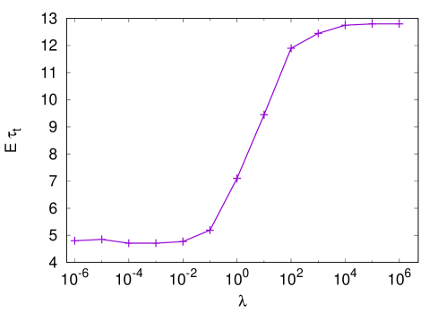
Figure 18: The scaled transient time scale $E\tau_{t}$ given by the numerical solution as a function of $\lambda$ for $E=10^{-6}$. The steady state is reached on a $O(E^{-1})$ time scale, both in the strongly and weakly stratified limits.

5 The flow in a polytropic envelope

5.1 The background

The next step towards a realistic model of the radiative envelope of a massive star is to include the strong density variations of the fluid between the convective core and the stellar surface. Typically density varies by a factor of $10^{9}$ in the envelope of a star of 15 solar masses. To take this density distribution into account in a simple way we assume that the gas can be described by a polytropic equation of state as usually done in stellar physics (e.g. Maeder, 2009). Hence the hydrostatic background state verifies:

$$-\frac{dp_{*}}{dr_{*}}-\frac{GM}{r_{*}^{2}}\rho_{*}=0\quad{\rm and}\quad\p_{*}=\kappa\rho_{*}^{\Gamma}\ ,$$ (90)

where $p_{*}$, $\rho_{*}$, and $r_{*}$ are the dimensional pressure, density, and radial coordinate, respectively. As previously, we also use the Roche approximation and assume that the core gathers all the mass $M$ of the star. In (90) $G$ is the gravitational constant, $\kappa$ is a constant related to the thermal conditions at the core boundary, and $\Gamma=1+1/n$, where $n$ is the so-called polytropic index. In the following we shall set $n=3$, which is typical for radiative envelopes. We note that for such an index the fluid is stably stratified (e.g. Dintrans & Rieutord, 2001; Rieutord & Dintrans, 2002, for instance), but as concluded from the previous section the small value of the Prandtl number allows us to neglect buoyancy effects. The following results therefore assume no buoyancy force.

Eq. (90) can be easily solved and gives the density profile

$$\rho_{*}(r_{*})=\rho_{c}(1+Bj(r_{*}))^{n}\ ,$$ (91)

where

$$B=\frac{\rho_{s}^{1/n}-1}{1/\eta-1},\qquad j(r_{*})=\frac{1}{\eta}-\frac{R}{r_{*}}\ .$$ (92)

Here $\rho_{c}=\rho_{*}(\eta R)$ is the density at the core boundary and $\rho_{s}=\rho_{*}(R)/\rho_{c}$ is the adimensional surface density. Note that such a background is also used in numerical simulations of convection in stellar envelope (Raynaud et al., 2018) or planetary atmospheres (Gastine & Wicht, 2012). Hence, in this section, we solve equations (1) with the background polytropic density profile (91), the boundary conditions (4), and with the initial condition ${\boldsymbol{u}}=\boldsymbol{0}$.

5.2 The transient phase

Again, we first focus on the transient phase preceding the settling of a steady-state. In particular, we aim at determining whether the scaling of the governing time scales are modified by density variations of the background. We measure the transient time as the time for which relative difference between the torque exerted by the fluid on the stationary inner sphere and the torque applied on the outer sphere, is less than $0.01\%$. We monitor the evolution of the relative difference between the torques $\Delta\Gamma/\Gamma(1)$ given by (18), for various surface density ratios. We show the resulting steady-state times in Fig. 19 for the polytropic indexes $n=3$ and $n=3/2$. The latter index corresponds to an isentropic monatomic gas, hence to a neutral thermal stratification. We find the steady state time to depend on the density ratio between the core and the surface. For the polytropic index $n=3$, relevant to the envelope of massive stars, we find $E\tau_{t}\propto\rho_{s}^{0.3}$ for $10^{-3}\leq\rho_{s}$, and $E\tau_{t}\propto\rho_{s}^{0.09}$ for $\rho_{s}<10^{-4}$. Of course, these power laws quantitatively depend on the chosen density profile, as can be seen with the $n=3/2$ case. Unlike thermal stratification, density stratification thus (mildly) influences the time scale required to reach a steady-state in a stellar envelope.

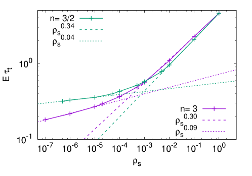
Figure 19: Scaled steady-state time scale $E\tau_{t}$ as a function of the surface density $\rho_{s}$, for $E=10^{-6}$ models with various values of $\rho_{s}$, $n=3/2$ and $n=3$. The dashed and dotted lines correspond to the steady-state time scalings with $\rho_{s}$.

5.3 The steady flow

We now focus on the steady flow. We may observe that if viscosity, non-linearity and buoyancy are neglected then the steady flow obeys a Taylor-Proudman theorem applied to the momentum $\rho{\boldsymbol{u}}$ instead of the velocity, namely

$$({\boldsymbol{e}}_{z}\cdot\boldsymbol{\nabla})\rho{\boldsymbol{u}}=\mathbf{0}\ .$$ (93)

Unfortunately we cannot reiterate the boundary layer analysis of the incompressible case since the viscous force (Eq. 3) now includes terms that depend on $r=\sqrt{s^{2}+z^{2}}$ and make the partial differential equation not separable. We may however observe that since the density variations do not add any new length scale, the viscous balance in the shear layers remains similar and we can still expect the presence of a Stewartson layer along the tangent cylinder.

We now revert to numerical solutions to make progress. We thus solve (1) with boundary condition (4). As already mentioned, we neglect the effects of buoyancy. We first focus on the differential rotation and the meridional circulation. It is convenient to introduce the stream function $\chi$ associated with the meridional momentum, namely

$$\frac{\partial\chi}{\partial r}=r\sin\theta\rho u_{\theta},\quad\quad\frac{\partial\chi}{\partial\theta}=-r^{2}\sin\theta\rho u_{r}\ .$$ (94)

Fig. 20 shows the differential rotation and this new stream function in the rotating frame of reference for $E=10^{-7}$.

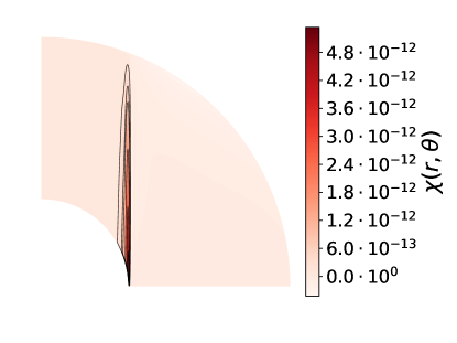
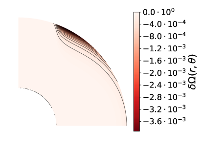
Figure 20: Meridional view of the stream function $\chi=\rho\psi$ (left) and of the differential rotation in the rotating frame of reference $\delta\Omega=(\Omega-\Omega_{c})/2\Omega_{c}$ (right) for $E=10^{-7}$, $\eta=0.35$, $\rho_{s}=10^{-4}$, and $A=0.01$.

We note that as for the incompressible flow, the amplitude of the secondary flow is dominated by the Stewartson layer located at the edge of the tangent cylinder $\mathcal{C}$. The differential rotation on the other hand, and as expected, is no longer cylindrical and very $z$-dependent, with a maximum value that is close to the outer shell and the tangent cylinder. Fig. 21a shows the differential rotation as a function of the cylindrical radial coordinate for $E=10^{-7}$ at different radii $r$, illustrating the $z$-dependence of $u_{\varphi}$, while Fig. 21b shows that $q_{\varphi}=\rho(r)u_{\varphi}$ verifies the Taylor-Proudman constraint.

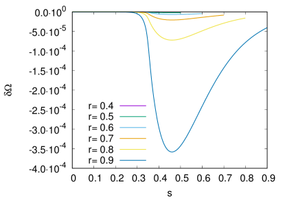
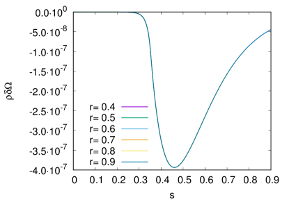
Figure 21: Normalised angular velocity (left) and normalised angular velocity multiplied by the density $\rho$ (right), and as a function of the cylindrical radial coordinate $s$ for $E=10^{-7}$, $\eta=0.35$, $\rho_{s}=10^{-4}$, $A=0.01$, and various radius.

As far as meridional circulation is concerned, this is still an ${\cal O}(E)$ flow outside the Stewartson layer as shown by Fig. 22a and 23a. We note that outside the tangent cylinder, streamlines are no longer straight lines, even for the ${\boldsymbol{q}}$ momentum field. In the inner cylinder and near the rotation axis we still get streamlines parallel to the rotation axis for the momentum ${\boldsymbol{q}}$. This latter feature comes from the fact that the Ekman layer has the same structure as in the constant density case and drives an Ekman circulation which has a unique component along the $z$-axis. From, Eq. 47 we deduce that

$$q_{z}=-\frac{EK\rho_{s}}{\sqrt{1-s^{2}}}\left(1+\frac{1}{1-s^{2}}\right)+O(E^{2})$$

in this region.

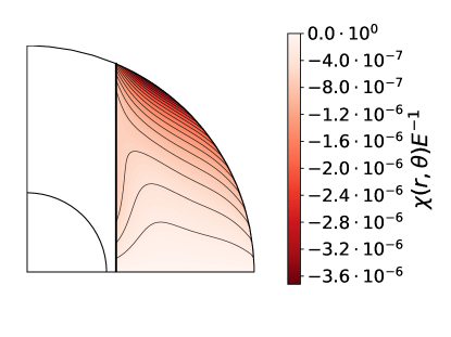
Figure 22: Left: $\chi E^{-1}$ as a function of the cylindrical radial coordinate $s$ for various Ekman numbers, $\eta=0.35$, $r=0.7$, $\rho_{s}=10^{-4}$, and $A=0.01$. The predicted $O(E)$ scaling of the secondary flow is verified away from the Stewartson nested layers. Right: Meridional view of the stream function $\chi E^{-1}$ outside $\mathcal{C}$, for the $E=10^{-9}$ model.

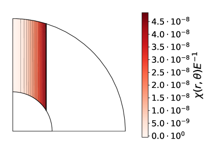
Figure 23: Left: $u_{z}E^{-1}$ as a function of the cylindrical radial coordinate $s$ for various Ekman numbers, $\eta=0.35$, $r=0.7$, $\rho_{s}=10^{-4}$, and $A=0.01$. Right: Meridional view of the stream function $\chi$ inside $\mathcal{C}$ and away from the $O(E^{2/7})$ Stewartson layer, for the $E=10^{-9}$ model.

Finally, the Stewartson layer seems to conserve its structure if we focus on the momentum, as shown by Figs 24 and 25. Hence, the $E^{1/3}$ scale is still the dominating scale.

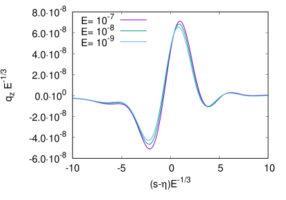
Figure 24: $q_{s}E^{-2/3}$ (left) and $q_{z}E^{-1/3}$ (right) as a function of the stretched cylindrical radial coordinate $(s-\eta)E^{-1/3}$ for various Ekman numbers, $\eta=0.35$, $z=0.7$, $\rho_{s}=10^{-4}$, and $A=0.01$.

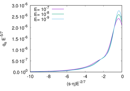
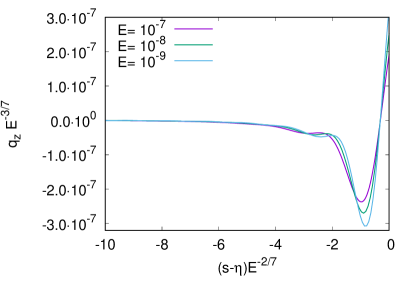
Figure 25: $q_{s}E^{-5/7}$ (left) and $q_{z}E^{-3/7}$ (right) as a function of the stretched cylindrical radial coordinate $(s-\eta)E^{-2/7}$ for various Ekman numbers, $\eta=0.35$, $z=0.7$, $\rho_{s}=10^{-4}$, and $A=0.01$.

6 Summary and conclusions

Aiming at a better description of the dynamics of the radiative envelopes of massive stars, which lose both mass and angular momentum through radiative winds, we have considered the problem of the spin-down flow of a viscous fluid inside a spherical shell. The spin-down is assumed to be driven by a tangential stress prescribed on the outer shell. This problem is quite close to the classical spherical Couette flow (Zikanov, 1996; Rieutord et al., 2012), but includes new features like density and thermal stratification, or stress driving, that needed new investigations.

To start with, we therefore considered this problem in the case of a mild driving so as to be able to deal with linear equations. After examining the case of constant density, we investigated the role of both density and thermal stable stratification. Since stars are large-size bodies, the Ekman number is very small. We therefore restricted our analysis to small Ekman numbers.

Our numerical solutions showed that the meridional kinetic energy is concentrated in the Stewartson shear layer that is tangent to the inner shell, both for incompressible and anelastic stationary flows assuming no thermal stratification. Outside this layer, a boundary layer analysis of the Ekman layers allowed us to exhibit analytical solutions for the quasi-geostrophic and incompressible primary and secondary stationary flows. We found the latter flow to be essentially perpendicular to the rotation axis outside the tangent cylinder, flowing from the outer Ekman layer towards the Stewartson layer. Inside the tangent cylinder, we found this poloidal flow to be parallel to the rotation axis, being pumped into the Ekman layer attached to the inner core. The mass-flux is then returned towards the outer Ekman layer through the Stewartson layer. Outside the Stewartson layer, the amplitude of the meridional flow (Ekman circulation) scales like $E$, as a consequence of the surface stress driving. In our model, the Stewartson layer is composed of two nested free shear layers of thickness $O(E^{2/7})$ and $O(E^{1/3})$. The analysis of the quasi-geostrophic $E^{2/7}$-layer located inside the tangent cylinder allowed us to derive asymptotic solutions for the primary and secondary flows, and a simple analysis of the ageostrophic $E^{1/3}$-layer indicates that it dominates the entire meridional circulation with a maximum amplitude of the $z$-directed velocity scaling as $E^{1/3}$.

We then accounted for a stable thermal stratification by introducing a radial temperature gradient using the Boussinesq approximation. Two limits of the parameter $\lambda=\Pran{\cal N}^{2}/(2\Omega_{c})^{2}$ show up. In the limit of strong thermal stratification, $\lambda\gg 1$, the angular velocity profile becomes shellular (only radially dependent), while the circulation is concentrated in thermal boundary layers and the radial motion is strongly inhibited outside of them. As a consequence, the Stewartson layer is suppressed. A more in-depth consideration of this regime, though certainly relevant to slowly rotating stars, has been deliberately left aside. Indeed, such slow rotators may never relax to a steady-state and thus might crucially depend on initial conditions. The study of the $\lambda\gg 1$ asymptotic regime, including the time-dependent baroclinic flow, certainly calls for a separate investigation. However, for rapidly rotating stars the relevant limit is $\lambda\ll 1$. In this case both the structure and amplitude of the incompressible and stationary flow are unaffected by the thermal stable stratification.

Radiative envelopes of massive stars exhibit however strong density variations between the convective core and the surface, making the incompressible and Boussinesq approximations too restrictive. But since thermal stratification has little impact for our stars, we can neglect buoyancy in the dynamics and concentrate on the effects of density stratification through the anelastic approximation. We chose to describe the gas of the stellar envelope by a polytropic equation of state with polytropic index $n=3$. We found that, assuming no further thermal stratification, the amplitude scaling of the stationary flow remains $O(E)$ outside the Stewartson layer and $O(E^{1/3})$ inside. However, outside the tangent cylinder, the streamlines are no longer straight lines and the flow becomes very dependent on the coordinate parallel to the rotation axis.

Because of the weakness of the meridional circulation, the stationary state of the flow is not quite relevant because it implies very long transients that might actually exceed the lifetime of the star. Massive stars are indeed short-lived (a few million years). We therefore checked the time scale associated with the transient phase and found it to be governed by the viscous diffusion time, that is $O(E^{-1})$ indeed. The density variations of the hydrostatic background seem to shorten it slightly. This implies that such a steady flow is typically reached on a time that is longer than the lifetime of the star. Fortunately, though the flow structure outside the tangent cylinder evolves during the transient, the dominating $E^{1/3}$ amplitude scaling of the meridional velocity stands. Hence, for all the models considered, the time relevant to the advective transport of chemicals within the radiative envelope of massive stars scales as $E^{-2/3}$, which is much shorter than the advection of angular momentum acting on $O(E^{-1})$ time scale.

The conclusion of the foregoing study is that the Stewartson layer is a key feature for the transport of chemical elements between the core and the surface of a massive star. The advective time scale is indeed $O(E^{-1/3})$ shorter than the spin-down time scale. In our case indeed, spin-down is driven by a stress and the steady state is reached on a viscous diffusion time, which is longer than the star’s life. The much shorter time associated with the meridional current of the Stewartson layer allows chemical elements produced in the core to be transported to the surface of the star and be possibly observable. We have shown that neither the stable stratification of the envelope, nor its strong density variations inhibit the rise of the Stewartson layer. The stable stratification is bypassed thanks to the low Prandtl number, while density variations have little influence on the mass flux $\rho{\boldsymbol{u}}$ basically because they occur on a large scale.

These conclusions are not the end of the story of course since other effects might complicate the scenario. The first effect one might think of is the local anisotropic turbulence of the envelope. Indeed, the differential rotation induces a local shear that is unstable. This shear instability is reduced by the stable stratification (Richarson criterion) but eased by the large heat diffusion. Zahn (1992) and Maeder & Zahn (1998) have argued that such instabilities will lead to a strongly anisotropic turbulence, making horizontal transport much more efficient than the vertical one. It is therefore an open question whether the Stewartson layer can resist to an anisotropic turbulent diffusion and in which circumstances.

If we still wish more realism, the interface between the core and the envelope will need a more detailed description. In this region, stable chemical stratification builds up in the course of stellar evolution. This so-called $\mu$-barrier might isolate the core from the envelope. However, the thermal gradient is still unstable and overstable double-diffusive convection is suspected to develop there (Garaud, 2020). The impact of rotation on the dynamics of this region is almost unknown and will also motivate future studies. Finally, magnetic fields, of fossil or core dynamo origin, may have a dramatic impact on massive stars interior dynamics. Indeed, depending on the field geometry, it can, for instance, amplify (Hollerbach, 1997) or suppress the Stewartson layer and yield a super-rotating jet (Kleeorin et al., 1997; Dormy et al., 1998). Their consideration is also a matter for future work.

Appendix A The linear approximation

A.1 Validity condition

This appendix presents an a posteriori justification for the use of linear approximation. For simplicity, we focus on the incompressible flow. In spherical coordinates and in the inertial frame, the non-linear dimensional momentum equation reads

$$\frac{\partial{\boldsymbol{u}}_{*}}{\partial t_{*}}+({\boldsymbol{u}}_{*}\cdot\boldsymbol{\nabla}){\boldsymbol{u}}_{*}=-\boldsymbol{\nabla}p_{*}+{\boldsymbol{F}}_{\rm visc}\ ,$$ (95)

where

$${\boldsymbol{F}}_{\rm visc}=\mu\left(\Delta{\boldsymbol{u}}_{*}+\frac{1}{3}\boldsymbol{\nabla}{\rm div}{\boldsymbol{u}}_{*}\right)+2(\boldsymbol{\nabla}\mu\cdot\boldsymbol{\nabla}){\boldsymbol{u}}_{*}+\boldsymbol{\nabla}\mu\times(\boldsymbol{\nabla}\times{\boldsymbol{u}}_{*})-\frac{2}{3}\boldsymbol{\nabla}(\mu{\rm div}{\boldsymbol{u}}_{*})$$ (96)

is the dimensional viscous force, and $\mu=\rho_{*}(r)\nu$ is the dynamical viscosity. Let us decompose the velocity field as the sum of the bulk component $\Omega_{c}{\boldsymbol{e}}_{z}\times{\boldsymbol{r}}$ and a residual velocity field ${\boldsymbol{u}}_{*}^{r}$

$${\boldsymbol{u}}_{*}=\Omega_{c}{\boldsymbol{e}}_{z}\times{\boldsymbol{r}}_{*}+{\boldsymbol{u}}_{*}^{r}\ .$$ (97)

For an axisymmetric flow, the non-linear term can be rewritten

$$({\boldsymbol{u}}_{*}\cdot\boldsymbol{\nabla}){\boldsymbol{u}}_{*}=\Omega_{c}^{2}{\boldsymbol{e}}_{z}\times({\boldsymbol{e}}_{z}\times r_{*})+2\Omega_{c}{\boldsymbol{e}}_{z}\times{\boldsymbol{u}}_{*}^{r}+({\boldsymbol{u}}_{*}^{r}\cdot\boldsymbol{\nabla}){\boldsymbol{u}}_{*}^{r}\ .$$ (98)

We further note that the centrifugal term derives from a potential that can be gathered with the pressure into $\Pi$. Finally, we write the non-linear adimensional momentum equation in the rotating frame

$$\frac{\partial{\boldsymbol{u}}^{r}}{\partial t}+({\boldsymbol{u}}^{r}\cdot\boldsymbol{\nabla}){\boldsymbol{u}}^{r}+{\boldsymbol{e}}_{z}\times{\boldsymbol{u}}^{r}=-\boldsymbol{\nabla}\Pi+E\Delta{\boldsymbol{u}}^{r}\ .$$ (99)

From now on the adimensional velocity field in the rotation frame ${\boldsymbol{u}}^{r}$ will be written ${\boldsymbol{u}}$ for simplicity. We now explicit the non-linear term as

$${\boldsymbol{u}}\cdot\boldsymbol{\nabla}{\boldsymbol{u}} =\begin{bmatrix}({\boldsymbol{u}}\cdot\boldsymbol{\nabla})u_{r}-(u_{\theta}^{2}+u_{\phi}^{2})/r\\ \\ ({\boldsymbol{u}}\cdot\boldsymbol{\nabla})u_{\theta}+(u_{\theta}u_{\phi}-u_{\phi}^{2}\cot\theta)/r\\ \\ ({\boldsymbol{u}}\cdot\boldsymbol{\nabla})u_{\phi}+(u_{r}u_{\phi}+u_{\theta}u_{\phi}\cot\theta)/r\end{bmatrix}\ .$$ (100)

The Ekman boundary layer analysis presented in Sect. 3.2.1 revealed $u_{r}$ and $u_{\theta}$ to be of order $E$ (except in the Stewartson layer). For an axisymmetric flow, and neglecting $O(E^{2})$ terms, (100) can be simplified as

$${\boldsymbol{u}}\cdot\boldsymbol{\nabla}{\boldsymbol{u}} =\begin{bmatrix}-u_{\phi}^{2}/r\\ \\ -u_{\phi}^{2}\cot\theta/r\\ \\ ({\boldsymbol{u}}\cdot\boldsymbol{\nabla})u_{\phi}+(u_{r}u_{\phi}+u_{\theta}u_{\phi}\cot\theta)/r\end{bmatrix}\ .$$ (101)

The Coriolis acceleration, in turn, reads

$${\boldsymbol{e}}_{z}\times{\boldsymbol{u}} =\begin{bmatrix}-\sin\theta u_{\phi}\\ \\ -\cos\theta u_{\phi}\\ \\ \cos\theta u_{\theta}+\sin\theta u_{r}\end{bmatrix}\ .$$ (102)

Since we work with the vorticity equation, we need

$$\boldsymbol{\nabla}\times({\boldsymbol{u}}\cdot\boldsymbol{\nabla}){\boldsymbol{u}} =\begin{bmatrix}1/(r\sin\theta)\partial_{\theta}\left[\sin\theta\left(({\boldsymbol{u}}\cdot\boldsymbol{\nabla})u_{\phi}+(u_{\phi}u_{r}+u_{\phi}u_{\theta})/r\right)\right]\\ \\ -1/r\partial_{r}\left[r({\boldsymbol{u}}\cdot\boldsymbol{\nabla})u_{\phi}+u_{\phi}u_{r}+u_{\phi}u_{\theta}\right]\\ \\ A_{\phi}\end{bmatrix}\ ,$$ (103)

and

$$\boldsymbol{\nabla}\times({\boldsymbol{e}}_{z}\times{\boldsymbol{u}}) =\begin{bmatrix}1/(r\sin\theta)\partial_{\theta}\left(\sin\theta\cos\theta u_{\theta}+\sin^{2}\theta u_{r}\right)\\ \\ -1/r\partial_{r}\left(r\cos\theta u_{\theta}+r\sin\theta u_{r}\right)\\ \\ B_{\phi}\end{bmatrix}\ ,$$ (104)

where

$$A_{\phi}=\frac{1}{r}\left(\frac{1}{r}\frac{\partial}{\partial\theta}-\cot\theta\frac{\partial}{\partial r}\right)u_{\phi}^{2}=-\frac{2u_{\phi}}{r^{2}}(s+z\cot\theta)\frac{\partial u_{\phi}}{\partial z}\ ,$$ (105)

and

$$B_{\phi}=\frac{1}{r}\left(\partial_{\theta}\sin\theta-\partial_{r}r\cos\theta\right)u_{\phi}=-\frac{\partial u_{\phi}}{\partial z}\ .$$ (106)

We note that in the steady-state, outside boundary layers $\partial u_{\phi}/\partial z=O(E)$ according to the Taylor-Proudman theorem, we can thus write the amplitude scaling of both terms

$$\mathinner{\!\left\lVert\boldsymbol{\nabla}\times({\boldsymbol{e}}_{z}\times{\boldsymbol{u}})\right\rVert}=\mathinner{\!\left\lVert\frac{\partial{\boldsymbol{u}}}{\partial z}\right\rVert}=O(E)\quad{\rm and}\quad\mathinner{\!\left\lVert\boldsymbol{\nabla}\times({\boldsymbol{u}}\cdot\boldsymbol{\nabla}){\boldsymbol{u}}\right\rVert}=O(u_{\phi}E)\ .$$ (107)

Hence, if $u_{\phi}=O(1)$ non-linear terms in the vorticity equation are of the same order as the curl of the Coriolis acceleration and therefore cannot be neglected. However, inside the tangent cylinder, we have found, in Sect. 3.2.2, that $u_{\phi}=O(\sqrt{E})$. In that region the non-linear terms can be neglected. Outside the tangent cylinder, the amplitude of the azimuthal velocity scales as $A$ (see eq. 29), and the non-linear terms are therefore $O(AE)$. Hence, for sufficiently small $A$, we expect the linear approximation to be relevant to our problem. We show the ratio between the Euclidian norm of (103) and that of (104) calculated a posteriori, for $A=0.01$ and $A=1$, in Fig. 26. We find, as expected, this ratio to be of order $A$ outside the tangent cylinder. The linear solution can therefore be considered as a good approximation to the non-linear and incompressible vorticity equation provided $A\ll 1$.

Figure 26: Meridional view of the ratio between the Euclidian norm of the vorticity equation non-linear term and that of the curl of the Coriolis acceleration, for $A=0.01$ (left) and $A=1$ (right), and for an incompressible flow.

Similarly, for the anelastic flow, we find

$$\frac{\mathinner{\!\left\lVert\boldsymbol{\nabla}\times\rho({\boldsymbol{u}}\cdot\boldsymbol{\nabla}){\boldsymbol{u}}\right\rVert}}{\mathinner{\!\left\lVert\boldsymbol{\nabla}\times({\boldsymbol{e}}_{z}\times\rho{\boldsymbol{u}})\right\rVert}}=O(u_{\phi})\ ,$$ (108)

where this time $u_{\phi}=O(A\rho_{s})$ outside the tangent cylinder. Since $\rho_{s}\ll 1$, the conditions of linearity are more easily met.

A.2 Application to massive stars

Let us now determine a typical value for $A$ when considering the differential rotation to be driven by a radiative wind at the surface of a massive star. We consider the outwardly accelerated outer layers to exert a viscous stress on the underlying layers of the star, spinning them down. Hence, we assume the local vertical angular momentum flux from the outwardly accelerated flow at the stellar surface to amount for the torque applied to the inner layers of the stars. That is

$$\dot{\ell}_{z}=R\sin\theta\sigma_{r\phi,*}\ ,$$ (109)

where $\dot{\ell}_{z}\equiv\dot{m}\Omega_{s}(R\sin\theta)^{2}$ is the local angular momentum flux, $\dot{m}$ is the associated local mass-flux that is assumed isotropic, $R$ is the stellar radius, and $[\sigma_{*}]$ is the dimensional stress tensor. Combining the expression for the imposed azimuthal stress Eq. (4) with Eq. (109) yields the adimensional amplitude of the surface stress resulting from the outward angular momentum flux

$$A=\sqrt{\frac{4\pi}{3}}\frac{\dot{m}\Omega_{s}(\theta)R(\theta)}{2\Omega_{c}\rho_{s,*}(\theta)\nu}\ ,$$ (110)

where $\rho_{s,*}=\rho_{s}\rho_{c}$ is the dimensional surface density. We compute all quantities with the ESTER 2D code (Rieutord et al., 2016; Gagnier et al., 2019a) for a $15~{}M_{\odot}$ stellar model with a rotation period of one day and we assume a (turbulent) kinematic viscosity at the surface $\nu=10^{12}cm^{2}.s^{-1}$ (Zahn, 1992; Espinosa Lara & Rieutord, 2013). We plot the amplitude of the surface stress weighed by surface density $A\rho_{s}$ as a function of co-latitude in Fig. 27. We further note that rotating stars are not strictly spherically symmetric because of the centrifugal force, in particular when rotation is rapid. Hence, the stellar radius as well as the surface density have latitudinal dependencies. Besides the resulting slight variation on the stellar surface, we see that $A\rho_{s}$ is of the order $5\cdot 10^{-8}\ll 1$ for this model. Hence, according to the results of Sect. A.1, the linear approximation can be used to model massive stars losing angular momentum, provided the kinematic viscosity at the surface is no less than $\sim 10^{7}cm^{2}.s^{-1}$, a typical value in radiation-dominated surface layers of massive stars (Espinosa Lara & Rieutord, 2013).

Figure 27: Amplitude of the surface stress weighed by the adimensional surface density $A\rho_{s}$ resulting from the angular momentum outward flux, as a function of co-latitude, for a $15~{}M_{\odot}$ 2D ESTER stellar model rotating with a period of one day.

Appendix B Asymptotically strong thermal stratification regime

In this appendix, we study the case of strong temperature stratification, that is in the $\lambda\gg 1$ asymptotic regime. We have seen, in Sect. 4.2, that in this regime, both Ekman and thermal horizontal boundary layers coexist, with respective thickness of order $\sqrt{E}$ and $1/\sqrt{\lambda}$.

B.1 The steady flow

In the asymptotic regime of small Ekman numbers, we have seen that because $u_{\phi}=O(1)$, the temperature deviation from equilibrium is at most $O(1)$. Unlike the weakly stratified case however, the associated $O(E/\lambda)$ interior radial velocity is less than the $O(E)$ stratification independent Ekman pumping, and is therefore a consistent solution for the interior flow. Let us now write the dynamical variables in the interior, as a power expansion of the small parameter $1/\sqrt{\lambda}$ corresponding to the width of the thermal boundary layer, in the asymptotic regime of small Ekman numbers. They read

$$u_{r} =E(\frac{1}{\sqrt{\lambda}}u_{r,1}+\frac{1}{\lambda}u_{r,2}+...)$$ (111)

$$u_{\theta} =E(\frac{1}{\sqrt{\lambda}}u_{\theta,1}+\frac{1}{\lambda}u_{\theta,2}+...)$$

$$u_{\phi} =u_{\phi,0}+\frac{1}{\sqrt{\lambda}}u_{\phi,1}+...$$

$$\delta T =\delta T_{0}+\frac{1}{\sqrt{\lambda}}\delta T_{1}+...$$

$$p =p_{0}+\frac{1}{\sqrt{\lambda}}p_{1}+...\ .$$

Injecting (111) in the momentum equation then yields the $O(1)$ and $O(1/\sqrt{\lambda})$ interior equations, that is

$$u_{\phi,0}=\frac{\partial p_{0}}{\partial s}-s\delta T_{0},\quad z\delta T_{0}=\frac{\partial p_{0}}{\partial z},\quad{\rm and}\quad\left(\nabla^{2}-\frac{1}{s^{2}}\right)u_{\phi,0}=0,\ ,$$ (112)

and

$$u_{\phi,1}=\frac{\partial p_{1}}{\partial s}-s\delta T_{1},\quad z\delta T_{1}=\frac{\partial p_{1}}{\partial z},\quad{\rm and}\quad\left(\nabla^{2}-\frac{1}{s^{2}}\right)u_{\phi,1}=u_{s,1}\ .$$ (113)

Hence, for large values of $\lambda$, thermal stratification inhibits vertical motions in the interior, and the Ekman layer pumping/suction no longer controls the dynamics of the interior flow. The Taylor-Proudman is not verified and is replaced by the thermal wind equation

$$({\boldsymbol{e}}_{z}\cdot\boldsymbol{\nabla}){\boldsymbol{u}}={\boldsymbol{r}}\times\boldsymbol{\nabla}\delta T\ ,$$ (114)

to $O(E{\boldsymbol{u}})$, and the $O(1)$ azimuthal velocity can be obtained solving

$$\left(\nabla^{2}-\frac{1}{s^{2}}\right)u_{\phi}=0\ .$$ (115)

This yields, using boundary conditions (12)

$$u_{\phi}\simeq\frac{K}{3}\left(\frac{1}{r^{3}}-\frac{1}{\eta^{3}}\right)r\sin\theta\ .$$ (116)

Hence, at the lowest order, $\delta\Omega=u_{\phi}/(r\sin\theta)$ is shellular in the asymptotic regime of large $\lambda$. Fig. 28 shows the angular velocity radial profiles at $\theta=\pi/2$, for $E=10^{-7}$ and for various $\lambda$. We see that the asymptotic limit where the $O(1/\sqrt{\lambda})$ terms can be neglected corresponds to $\lambda\gtrsim 10^{4}$.

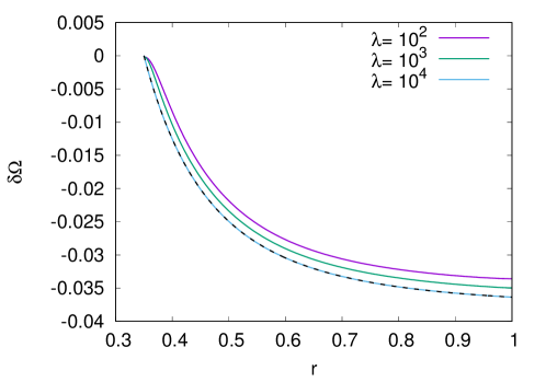
Figure 28: Angular velocity radial profiles in the rotating frame $\delta\Omega$, at $\theta=\pi/2$, $E=10^{-7}$, and for various $\lambda$. The black dashed line corresponds to the asymptotic solution (116).

Another interesting feature of the $\lambda\gg 1$ regime is that the circulation is concentrated in the boundary layers. This can be seen in Fig. 16 for $\lambda=10^{2}$. In the interior, the radial motion is so strongly inhibited by thermal stratification that it prevents the existence of the Stewartson layer, thus undermining rotation-induced advection.

In the thermal layers, radial gradients are increased by a factor $\sqrt{\lambda}$ which gives $\hat{u}_{r}=O(E)$, and from the continuity equation $\hat{u}_{\theta}=O(\sqrt{\lambda}E)$. In Fig. 29, we plot $u_{\theta}/(E\sqrt{\lambda})$ as a function of the stretched radial coordinate $(r-\eta)\sqrt{\lambda}$, for various combinations of Ekman numbers and $\lambda$ parameters. We find that, indeed, the latitudinal velocity scales as $\sqrt{\lambda E}$ in the outer part of the layer of thickness $\delta_{\lambda}$, that is in the thermal boundary layer region, outside the Ekman layer (typically for $(r-\eta)\sqrt{\lambda}\gtrsim 0.5$). Additionally, we verify the $O(\sqrt{E})$ amplitude scaling of the latitudinal velocity in the Ekman boundary layer. Indeed, Fig. 29 shows that provided fixed values of $\delta_{E}/\delta_{\lambda}$, that is fixed values of $\sqrt{\lambda E}$, the latitudinal velocity scales as $\sqrt{\lambda}E$ in the Ekman boundary layer as well. However, taking $\sqrt{\lambda E}=D$, where $D$ is some constant, implies that $\sqrt{\lambda}E=D\sqrt{E}$, hence $\hat{u}_{\theta}\propto\tilde{u}_{\theta}=O(\sqrt{E})$.

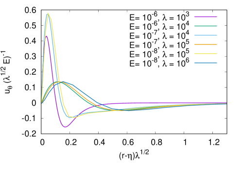
Figure 29: $u_{\theta}(\sqrt{\lambda}E)^{-1}$ as a function of the stretched radial coordinate $(r-\eta)\sqrt{\lambda}$, for various combinations of Ekman numbers and $\lambda$ parameters, $\eta=0.35$, $\theta=\pi/8$, and $A=0.01$.

B.2 The transient flow

We finally determine the scaling of the transient time with the Ekman number and the $\lambda$-parameter, in the $\lambda\gg 1$ limit. Assuming that in this regime, $\delta T$ remains $O(1)$ during the transient, (87) simplifies to

$$\frac{\partial}{\partial t}\left(\operatorname{cotan}\theta\frac{\partial}{\partial\theta}\tan\theta u_{\phi}\right)\simeq E\operatorname{cotan}\theta\frac{\partial}{\partial\theta}\tan\theta\left(\nabla^{2}-\frac{1}{r^{2}\sin^{2}\theta}\right)u_{\phi}\ ,$$ (117)

indicating that the (non-geostrophic) steady-state is reached on a $O(E^{-1})$ time scale as well. This is verified in Fig. 18. We note a weak $\lambda$ dependence of this time scale in the intermediate stratification regime.

References

- Barcilon (1968) Barcilon, V. 1968 Stewartson layers in transient rotating fluid flows. Journal of Fluid Mechanics 33, 815–825.
- Barcilon & Pedlosky (1967) Barcilon, V. & Pedlosky, J. 1967 A unified linear theory of homogeneous and stratified rotating fluids. Journal of Fluid Mechanics 29, 609–621.
- Brandenburg et al. (1996) Brandenburg, A., Jennings, R., Nordlund, Å., Rieutord, M., Stein, R. F. & Tuominen, I. 1996 Magnetic structures in a dynamo simulation. J. Fluid Mech. 306, 325–357.
- Chaboyer & Zahn (1992) Chaboyer, B. & Zahn, J.-P. 1992 Effect of horizontal turbulent diffusion on transport by meridional circulation. A&A 253, 173–177.
- Chandrasekhar (1961) Chandrasekhar, S. 1961 Hydrodynamic and hydromagnetic stability. Clarendon Press, Oxford.
- Dintrans & Rieutord (2001) Dintrans, B. & Rieutord, M. 2001 A comparison of the anelastic and subseismic approximations for low-frequency gravity modes in stars. MNRAS 324, 635–642.
- Dormy et al. (1998) Dormy, E., Cardin, P. & Jault, D. 1998 MHD flow in a slightly differentially rotating spherical shell, with conducting inner core, in a dipolar magnetic field. Earth and Planetary Science Letters 160, 15–30.
- Espinosa Lara & Rieutord (2011) Espinosa Lara, F. & Rieutord, M. 2011 Gravity darkening in rotating stars. A&A 533, A43.
- Espinosa Lara & Rieutord (2013) Espinosa Lara, F. & Rieutord, M. 2013 Self-consistent 2D models of fast rotating early-type stars. A&A 552, A35.
- Friedlander (1976) Friedlander, S. 1976 Quasi-steady flow of a rotating stratified fluid in a sphere. J. Fluid Mech. 76, 209–228.
- Gagnier & Garaud (2018) Gagnier, D. & Garaud, P. 2018 Turbulent Transport by Diffusive Stratified Shear Flows: From Local to Global Models. II. Limitations of Local Models. ApJ 862, 36, arXiv: 1803.10455.
- Gagnier et al. (2019a) Gagnier, D., Rieutord, M., Charbonnel, C., Putigny, B. & Espinosa Lara, F. 2019a Critical angular velocity and anisotropic mass loss of rotating stars with radiation-driven winds. A&A 625, A88.
- Gagnier et al. (2019b) Gagnier, D., Rieutord, M., Charbonnel, C., Putigny, B. & Espinosa Lara, F. 2019b Evolution of rotation in rapidly rotating early-type stars during the main sequence with 2D models. A&A 625, A89.
- Garaud (2002) Garaud, P. 2002 On rotationally driven meridional flows in stars. MNRAS 335, 707–711.
- Garaud (2020) Garaud, P. 2020 Double-diffusive processes in stellar astrophysics. In Multi-Dimensional Processes In Stellar Physics. Edts M. Rieutord, I. Baraffe & Y. Lebreton, p. 13.
- Garaud et al. (2017) Garaud, P., Gagnier, D. & Verhoeven, J. 2017 Turbulent Transport by Diffusive Stratified Shear Flows: From Local to Global Models. I. Numerical Simulations of a Stratified Plane Couette Flow. ApJ 837, 133, arXiv: 1610.04320.
- Gastine & Wicht (2012) Gastine, T. & Wicht, J. 2012 Effects of compressibility on driving zonal flow in gas giants. Icarus 219 (1), 428–442.
- Georgy et al. (2011) Georgy, C., Meynet, G. & Maeder, A. 2011 Effects of anisotropic winds on massive star evolution. A&A 527, A52, arXiv: 1011.6581.
- Goldstein (1938, 1965) Goldstein, S. 1938, 1965 Modern developments in Fluid Dynamics. Clarendon Press, Oxford, Dover.
- Greenspan (1968) Greenspan, H. P. 1968 The Theory of Rotating Fluids. Cambridge University Press.
- Hollerbach (1994) Hollerbach, R. 1994 Magnetohydrodynamic Ekman and Stewartson layers in a rotating spherical shell. Proc. R. Soc. Lond. 444, 333.
- Hollerbach (1997) Hollerbach, R. 1997 The influence of an axial field on magnetohydrodynamic ekman and stewartson layers, in the presence of a finitely conducting inner core. Acta Astronomica Geophysica Universitatis Comenianae 19, 263–275.
- Hypolite et al. (2018) Hypolite, D., Mathis, S. & Rieutord, M. 2018 The 2D dynamics of radiative zones of low-mass stars. A&A 610, A35, arXiv: 1711.08544.
- Hypolite & Rieutord (2014) Hypolite, D. & Rieutord, M. 2014 Dynamics of the envelope of a rapidly rotating star or giant planet in gravitational contraction. A&A 572, A15.
- Jones et al. (2009) Jones, C. A., Kuzanyan, K. M. & Mitchell, R. H. 2009 Linear theory of compressible convection in rapidly rotating spherical shells, using the anelastic approximation. J. Fluid Mech. 634, 291.
- Käpylä et al. (2012) Käpylä, Petri J., Mantere, Maarit J. & Brandenburg, Axel 2012 Cyclic Magnetic Activity due to Turbulent Convection in Spherical Wedge Geometry. ApJ Lett. 755 (1), L22.
- Kleeorin et al. (1997) Kleeorin, N., Rogachevskii, I., Ruzmaikin, A., Soward, A. M. & Starchenko, S. 1997 Axisymmetric flow between differentially rotating spheres in a dipole magnetic field. Journal of Fluid Mechanics 344 (1), 213–244.
- Kudritzki et al. (1987) Kudritzki, R. P., Pauldrach, A. & Puls, J. 1987 Radiation driven winds of hot luminous stars. II - Wind models for O-stars in the Magellanic Clouds. A&A 173, 293–298.
- Kulenthirarajah & Garaud (2018) Kulenthirarajah, L. & Garaud, P. 2018 Turbulent Transport by Diffusive Stratified Shear Flows: From Local to Global Models. III. A Closure Model. ApJ 864, 107, arXiv: 1803.11530.
- Lee et al. (2014) Lee, U., Neiner, C. & Mathis, S. 2014 Angular momentum transport by stochastically excited oscillations in rapidly rotating massive stars. MNRAS 443, 1515–1522, arXiv: 1404.5133.
- Maeder (2009) Maeder, A. 2009 Physics, Formation and Evolution of Rotating stars. Springer.
- Maeder & Meynet (2000) Maeder, A. & Meynet, G. 2000 Stellar evolution with rotation. VI. The Eddington and Omega -limits, the rotational mass loss for OB and LBV stars. A&A 361, 159–166, arXiv: astro-ph/0006405.
- Maeder & Zahn (1998) Maeder, A. & Zahn, J. P. 1998 Stellar evolution with rotation. iii. meridional circulation with mu -gradients and non-stationarity. A&A 334, 1000–1006.
- Marcotte et al. (2016) Marcotte, F., Dormy, E. & Soward, A. 2016 On the equatorial Ekman layer. Journal of Fluid Mechanics 803, 395–435, arXiv: 1602.08647.
- Meynet & Maeder (1997) Meynet, G. & Maeder, A. 1997 Stellar evolution with rotation. I. The computational method and the inhibiting effect of the -gradient. A&A 321, 465–476.
- Moore & Saffman (1968) Moore, D. & Saffman, P. 1968 The rise of a body through a rotating fluid in a container of finite length. J. Fluid Mech. 31, 635–642.
- Paxton et al. (2011) Paxton, B., Bildsten, L., Dotter, A., Herwig, F., Lesaffre, P. & Timmes, F. 2011 Modules for Experiments in Stellar Astrophysics (MESA). Astrophys. J. Supp. Ser. 192, 3.
- Pelupessy et al. (2000) Pelupessy, I., Lamers, H. J. G. L. M. & Vink, J. S. 2000 The radiation driven winds of rotating B[e] supergiants. A&A 359, 695–706, arXiv: astro-ph/0005300.
- Prat et al. (2016) Prat, V., Guilet, J., Viallet, M. & Müller, E. 2016 Shear mixing in stellar radiative zones. II. Robustness of numerical simulations. A&A 592, A59, arXiv: 1512.04223.
- Prat & Lignières (2013) Prat, V. & Lignières, F. 2013 Turbulent transport in radiative zones of stars. A&A 551, L3, arXiv: 1301.4151.
- Prat & Lignières (2014) Prat, V. & Lignières, F. 2014 Shear mixing in stellar radiative zones. I. Effect of thermal diffusion and chemical stratification. A&A 566, A110, arXiv: 1404.6199.
- Proudman (1956) Proudman, I. 1956 The almost-rigid rotation of viscous fluid between concentric spheres. Journal of Fluid Mechanics 1, 505–516.
- Proudman (1916) Proudman, J. 1916 On the Motion of Solids in a Liquid Possessing Vorticity. Proceedings of the Royal Society of London Series A 92, 408–424.
- Puls et al. (2000) Puls, J., Springmann, U. & Lennon, M. 2000 Radiation driven winds of hot luminous stars. XIV. Line statistics and radiative driving. A & A Suppl. Ser. 141, 23–64.
- Puls et al. (2008) Puls, J., Vink, J. S. & Najarro, F. 2008 Mass loss from hot massive stars. A&A Review 16, 209–325, arXiv: 0811.0487.
- Raynaud et al. (2018) Raynaud, R., Rieutord, M., Petitdemange, L., Gastine, T. & Putigny, B. 2018 Gravity darkening in late-type stars. I. The Coriolis effect. A&A 609, A124.
- Rieutord (1987) Rieutord, M. 1987 Linear theory of rotating fluids using spherical harmonics. I. Steady flows. Geophys. Astrophys. Fluid Dyn. 39, 163.
- Rieutord (2006) Rieutord, M. 2006 The dynamics of the radiative envelope of rapidly rotating stars. i. a spherical boussinesq model. A&A 451, 1025–1036.
- Rieutord & Beth (2014) Rieutord, M. & Beth, A. 2014 Dynamics of the radiative envelope of rapidly rotating stars: Effects of spin-down driven by mass loss. A&A 570, A42.
- Rieutord & Dintrans (2002) Rieutord, M. & Dintrans, B. 2002 More about the anelastic and subseismic approximations for low-frequency modes in stars. to be submitted to MNRAS 0, 1–5.
- Rieutord et al. (2016) Rieutord, M., Espinosa Lara, F. & Putigny, B. 2016 An algorithm for computing the 2D structure of fast rotating stars. Journal of Computational Physics 318, 277–304, arXiv: 1605.02359.
- Rieutord et al. (2012) Rieutord, M., Triana, S. A., Zimmerman, D. S. & Lathrop, D. P. 2012 Excitation of inertial modes in an experimental spherical Couette flow. Phys. Rev. E 86 (2), 026304.
- Rieutord & Valdettaro (1997) Rieutord, M. & Valdettaro, L. 1997 Inertial waves in a rotating spherical shell. J. Fluid Mech. 341, 77–99.
- Roberts & Stewartson (1963) Roberts, P. & Stewartson, K. 1963 On the stability of a Maclaurin spheroid of small viscosity. ApJ 137, 777–790.
- Rogers et al. (2013) Rogers, T. M., Lin, D. N. C., McElwaine, J. N. & Lau, H. H. B. 2013 Internal Gravity Waves in Massive Stars: Angular Momentum Transport. ApJ 772, 21.
- Stewartson (1966) Stewartson, K. 1966 On almost rigid rotations. part 2. J. Fluid Mech. 26, 131–144.
- Taylor (1921) Taylor, G. I. 1921 Experiments with Rotating Fluids. Proceedings of the Royal Society of London Series A 100, 114–121.
- Zahn (1974) Zahn, J.-P. 1974 Rotational instabilities and stellar evolution. In IAU Symp. 59: Stellar Instability and Evolution, pp. 185–194.
- Zahn (1992) Zahn, J.-P. 1992 Circulation and turbulence in rotating stars. A&A 265, 115–132.
- Zikanov (1996) Zikanov, O. Yu. 1996 Symmetry-breaking bifurcations in spherical Couette flow. J. Fluid Mech. 310, 293–324.