Steepest Neural Architecture Descent: Escaping Local Optimum with Signed Neuron Splittings

Abstract

Developing efficient and principled neural architecture optimization methods is a critical challenge of modern deep learning. Recently, Liu et al. [19] proposed a splitting steepest descent (S2D) method that jointly optimizes the neural parameters and architectures based on progressively growing network structures by splitting neurons into multiple copies in a steepest descent fashion. However, S2D suffers from a local optimality issue when all the neurons become “splitting stable”, a concept akin to local stability in parametric optimization. In this work, we develop a significant and surprising extension of the splitting descent framework that addresses the local optimality issue. The idea is to observe that the original S2D is unnecessarily restricted to splitting neurons into positive weighted copies. By simply allowing both positive and negative weights during splitting, we can eliminate the appearance of splitting stability in S2D and hence escape the local optima to obtain better performance. By incorporating signed splittings, we significantly extend the optimization power of splitting steepest descent both theoretically and empirically. We verify our method on various challenging benchmarks such as CIFAR-100, ImageNet and ModelNet40, on which we outperform S2D and other advanced methods on learning accurate and energy-efficient neural networks.

1 Introduction

Although the parameter learning of deep neural networks (DNNs) has been well addressed by gradient-based optimization, efficient optimization of neural network architectures (or structures) is still largely open. Traditional approaches frame the neural architecture optimization as a discrete combinatorial optimization problem, which, however, often lead to highly expensive computational cost and give no rigorous theoretical guarantees. New techniques for efficient and principled neural architecture optimization can significantly advance the-state-of-the-art of deep learning.

Recently, Liu et al. [19] proposed a splitting steepest descent (S2D) method for efficient neural architecture optimization, which frames the joint optimization of the parameters and neural architectures into a continuous optimization problem in an infinite dimensional model space, and derives a computationally efficient (functional) steepest descent procedure for solving it. Algorithmically, S2D works by alternating between typical parametric updates with the architecture fixed, and an architecture descent which grows the neural network structures by optimally splitting critical neurons into a convex combination of multiple copies.

In S2D, the optimal rule for picking what neurons to split and how to split is theoretically derived to yield the fastest descent of the loss in an asymptotically small neighborhood. Specifically, the optimal way to split a neuron is to divide it into two equally weighted copies along the minimum eigen-direction of a key quantity called splitting matrix for each neuron. Splitting a neuron into more than two copies can not introduce any additional gain theoretically and do not need to be considered for computational efficiency. Moreover, the change of loss resulted from splitting a neuron equals the minimum eigen-value of its splitting matrix (called the splitting index). Therefore, neurons whose splitting matrix is positive definite are considered to be “splitting stable” (or not splittable) in that splitting them in any fashion can increase the loss and hence would be “pushed back” by subsequent gradient descent. In this way, the role of splitting matrices is analogous to how Hessian matrices characterize local stability for typical parametric optimization, and the local stability due to positive definite splitting matrices can be viewed as a notation of local optimality in the parameter-structure joint space. Unfortunately, the presence of the splitting stable status leads to a key limitation of the practical performance of splitting steepest descent, since the loss can be stuck at a relatively large value when the splittings become stable and can not continue.

This work fills a surprising missing piece of the picture outlined above, which allows us to address the local optimality problem in splitting descent with a simple algorithmic improvement. We show that the notation of splitting stable caused by positive definite splitting matrices is in fact an artifact of splitting neurons into positively weighted copies. By simply considering signed splittings which allows us to split neurons into copies with both positive and negative weights, the loss can continue decrease unless the splitting matrices equals zero for all the neurons. Intriguingly, the optimal spitting rules with signed weights can have upto three or four copies (a.k.a. triplet and quartet splittings; see Figure 4(c-e)), even though signed binary splittings (Figure 4(a-b)), which introduces no additional neurons over the original positively weighted splitting, can work sufficiently well in practice.

Our main algorithm, signed splitting steepest descent (S3D), which outperforms the original S2D in both theoretical guarantees and empirical performance. Theoretically, it yields stronger notion of optimality and allows us to establish convergence analysis that was impossible for S2D. Empirically, S3D can learn smaller and more accurate networks in a variety of challenging benchmarks, including CIFAR-100, ImageNet, ModelNet40, on which S3D substantially outperforms S2D and a variety of baselines for learning small and energy-efficient networks [e.g. 20, 17, 13, 15].

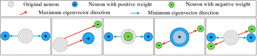
(a) Positive Binary Splitting

(b) Negative Binary Splitting

(c) Positive Triplet Splitting

(d) Negative Triplet Splitting

(e) Quartet Splitting

Figure 1: Different splitting strategies. The original splitting steepest descent [19] only uses positive binary splitting (a), which splits the neuron into two positively weighted copies. By allowing the neurons to split into output weighted by negative weights, we derive a host of new splitting rules (b,c,d,e), which can descent the loss more optimally, and avoid the appearance of splitting stability due to positive splitting matrices. In practice, we find that the combination of positive and negative binary splittings (a-b) works sufficiently well.

2 Background: Splitting Steepest Descent

Following Liu et al. [19], we start with the case of splitting a single-neuron network $f(x)=\sigma(\theta,x)$, where $\theta\in\mathbb{R}^{d}$ is the parameter and $x$ the input. On a data distribution $\mathcal{D}$, the loss function of $\theta$ is

$$L(\theta)=\mathbb{E}_{x\sim\mathcal{D}}\left[\Phi\left(\sigma(\theta,x)\right)\right],$$

where $\Phi(\cdot)$ denotes a nonlinear loss function.

Assume we split a neuron with parameter $\theta$ into $m$ copies whose parameters are $\{\theta_{i}\}_{i=1}^{m}$, each of which is associated with a weight $w_{i}\in\mathbb{R}$, yielding a large neural network of form $f(x)=\sum_{i}w_{i}\sigma(\theta_{i},x)$. Its loss function is

$${\mathcal{L}_{m}}(\boldsymbol{\theta},\boldsymbol{w})=\mathbb{E}_{x\sim\mathcal{D}}\left[\Phi\left(\sum_{i=1}^{m}w_{i}\sigma(\theta_{i},x)\right)\right],$$

where we write $\boldsymbol{\theta}=\{\theta_{i}\}_{i=1}^{m}$ $\boldsymbol{w}:=\{w_{i}\}_{i=1}^{m}$. We shall assume $\sum_{i}w_{i}=1$, so that we obtain an equivalent network, or a network morphism [35], when the split copies are not updated, i.e., $\theta_{i}=\theta$ for $\forall i$. We want to find the optimal splitting scheme ($\boldsymbol{\theta}$, $\boldsymbol{w}$, $m$) to yield the minimum loss ${\mathcal{L}_{m}}(\boldsymbol{\theta},\boldsymbol{w})$.

Assume the copies $\{\theta_{i}\}$ can be decomposed into $\theta_{i}=\theta+\epsilon(\delta_{0}+\delta_{i})$ where $\epsilon$ denotes a step-size parameter, $\delta_{0}:=\sum_{i}w_{i}\theta_{i}-\theta$ the average displacement of all copies (which implies $\sum_{i}w_{i}\delta_{i}=0$), and $\theta_{i}$ the individual “splitting” direction of $\theta_{i}$. Liu et al. [19] showed the following key decomposition:

$${\mathcal{L}_{m}}(\boldsymbol{\theta},\boldsymbol{w})=L(\theta+\epsilon\delta_{0})+\frac{\epsilon^{2}}{2}{\Pi_{m}}(\boldsymbol{\delta},\boldsymbol{w};\theta)+O(\epsilon^{3}),$$ (1)

where $L(\theta+\epsilon\delta_{0})$ denotes the effect of average displacement, corresponding to typical parametric $\theta\mapsto\theta+\epsilon\delta_{0}$ without splitting, and ${\Pi_{m}}(\boldsymbol{\delta},\boldsymbol{w};\leavevmode\nobreak\ \theta)$ denotes the effect of splitting the neurons; it is a quadratic form depending on a splitting matrix defined in Liu et al. [19]:

$$\begin{split}{\Pi_{m}}(\boldsymbol{\delta},\boldsymbol{w};\leavevmode\nobreak\ \theta)=\sum_{i=1}^{m}w_{i}\delta_{i}^{\top}S(\theta)\delta_{i},\leavevmode\nobreak\ \leavevmode\nobreak\ \leavevmode\nobreak\ \leavevmode\nobreak\ \leavevmode\nobreak\ \leavevmode\nobreak\ \leavevmode\nobreak\ \text{where\leavevmode\nobreak\ \leavevmode\nobreak\ \leavevmode\nobreak\ \leavevmode\nobreak\ }S(\theta)&=\mathbb{E}_{x\sim\mathcal{D}}[\Phi^{\prime}(\sigma(\theta,x))\nabla_{\theta\theta}^{2}\sigma(\theta,x)].\end{split}$$ (2)

Here $S(\theta)\in\mathbb{R}^{d\times d}$ is called the splitting matrix of $L(\theta)$. Because splitting increases the number of neurons and only contributes an $O(\epsilon^{2})$ decrease of loss following (1), it is preferred to decrease the loss with typical parametric updates that requires no splitting (e.g., gradient descent), whenever the parametric local optimum of $L(\theta)$ is not achieved. However, when we research a local optimum of $L(\theta)$, splitting allows us to escape the local optimum at the cost of increasing the number of neurons. In Liu et al. [19], the optimal splitting scheme is framed into an optimization problem:

$$G_{m}^{+}:=\min_{\boldsymbol{\delta},\boldsymbol{w}}\left\{{\Pi_{m}}(\boldsymbol{\delta},\boldsymbol{w};\theta)\colon\leavevmode\nobreak\ \boldsymbol{w}\in P_{m}^{+},\leavevmode\nobreak\ \boldsymbol{\delta}\in{\Delta}_{\boldsymbol{w}}\right\},$$ (3)

where we optimize the weights $\boldsymbol{w}$ in a probability simplex $P_{m}^{+}$ and splitting vectors $\boldsymbol{\delta}$ in set set $\Delta_{\boldsymbol{w}}$:

$$P_{m}^{+}=\big{\{}\boldsymbol{w}\in\mathbb{R}^{m}\colon\leavevmode\nobreak\ \sum_{i=1}^{m}w_{i}=1,\leavevmode\nobreak\ w_{j}\geq 0,\leavevmode\nobreak\ \leavevmode\nobreak\ \forall j\big{\}},$$ (4)

$$\Delta_{\boldsymbol{w}}=\big{\{}\boldsymbol{\delta}\in\mathbb{R}^{m\times d}\colon\sum_{i=1}^{m}w_{i}\delta_{i}=0,\leavevmode\nobreak\ \left\lVert\delta_{j}\right\rVert\leq 1,\leavevmode\nobreak\ \forall j\big{\}},$$

in which $\delta_{i}$ is constrained in the unit ball and the constraint $\sum_{i=1}^{m}w_{i}\delta_{i}=0$ is to ensure a zero average displacement. Liu et al. [19] showed that the optimal gain $G_{m}^{+}$ in (3) depends on the minimum eigen-value $\lambda_{\min}$ of $S(\theta)$ in that

$$G_{m}^{+}=\min\left(\lambda_{\min},0\right).$$

If $\lambda_{\min}<0$, we obtain a strict decrease of the loss, and the maximum decrease can be achieved by a simple binary splitting scheme ($m=2$), in which the neuron is split into two equally weighted copies along the minimum eigen-vector direction $v_{\min}$ of $S(\theta)$, that is,

$$m=2, w_{1}=w_{2}=1/2, \delta_{1}=-\delta_{2}=v_{\min}.$$ (5)

See Figure 1(a) for an illustration. This binary splitting $(m=2)$ defines the best possible splitting in the sense of (3), which means that it can not be further improved even when it is allowed to split the neuron into an arbitrary number $m$ of copies.

On the other hand, if $\lambda_{\min}>0$, we have $G_{m}^{+}=0$ and the loss can not be decreased by any splitting scheme considered in (3). This case was called being splitting stable in Liu et al. [19], which means that even if the neuron is split into an arbitrary number of copies in arbitrary way (with a small step size $\epsilon$), all its copies would be pushed back to the original neuron when gradient descent is applied subsequently.

2.1 Main Method: Signed Splitting Steepest Descent

Following the derivation above, the splitting process would get stuck and stop when the splitting matrix $S(\theta)$ is positive definite ($\lambda_{\min}>0$), and it yields small gain when $\lambda_{\min}$ is close to zero. Our key observation is that this phenomenon is in fact an artifact of constraining the weights $w_{i}$ to be non-negative in optimization (3)-(4). By allowing negative weights, we can open the door to a much richer class of splitting schemes, which allows us to descent the loss more efficiently. Interestingly, although the optimal positively weighted splitting is always achievable by the binary splitting scheme ($m=2$) shown in (5), the optimal splitting schemes with signed weights can be either binary splitting ($m=2$), triplet splitting ($m=3$), or at most quartet splitting ($m=4$).

Specifically, our idea is to replace (3) with

$$\!\!\!\!\!\!G_{m}^{-c}:=\min_{\boldsymbol{\delta},\boldsymbol{w}}\left\{{\Pi_{m}}(\boldsymbol{\delta},\boldsymbol{w};\theta)\colon\leavevmode\nobreak\ \boldsymbol{w}\in P_{m}^{-c},\leavevmode\nobreak\ \boldsymbol{\delta}\in{\Delta}_{\boldsymbol{w}}\right\},$$ (6)

where the weight $\boldsymbol{w}$ is constrained in a larger set $P_{m}^{-c}$ whose size depends on a scalar $c\in[1,\infty)$:

$$\!\!\!\!P_{m}^{-c}=\big{\{}\boldsymbol{w}\in\mathbb{R}^{m}\colon\sum_{i=1}^{m}w_{i}=1,\leavevmode\nobreak\ \sum_{i=1}^{m}|w_{i}|\leq c\big{\}}.$$ (7)

We can see that $P_{m}^{-c}$ reduces to $P_{m}^{+}$ when $c=1$, and contains negative weights when $c>1$. By using $c>1$, we enable a richer class of splitting schemes with signed weights, hence yielding faster descent of the loss function.

The optimization in (6) is more involved than the positive case (3), but still yield elementary solutions. We now discuss the solution when we split the neuron into $m=2,3,4$ copies, respectively. Importantly, we show that no additional gain can be made by splittings with more than $m=4$ copies.

For notation, we denote by $\lambda_{\min}$, $\lambda_{\max}$ the smallest and largest eigenvalues of $S(\theta)$, respectively, and $v_{\min}$, $v_{\max}$ their corresponding eigen-vectors with unit norm.

Theorem 2.1 (Binary Splittings).

For the optimization in (6) with $m=2$ and $c\geq 1$, we have

$$G_{2}^{-c}=\min\left(\lambda_{\min},\leavevmode\nobreak\ \leavevmode\nobreak\ -\frac{c-1}{c+1}\lambda_{\max},\leavevmode\nobreak\ \leavevmode\nobreak\ 0\right),$$

and the optimum is achieved by one of the following cases:

i) no splitting ($\delta_{1}=\delta_{2}=0$), which yields $G_{2}^{-c}=0$;

ii) the positive binary splitting in (5), yielding $G_{2}^{-c}=\lambda_{\min}$;

iii) the following “negative” binary splitting scheme:

$$\begin{split}w_{1}=-\frac{c-1}{2},\leavevmode\nobreak\ \leavevmode\nobreak\ \leavevmode\nobreak\ \leavevmode\nobreak\ \delta_{1}=v_{\max},\leavevmode\nobreak\ \leavevmode\nobreak\ \leavevmode\nobreak\ \leavevmode\nobreak\ \leavevmode\nobreak\ \leavevmode\nobreak\ \leavevmode\nobreak\ \leavevmode\nobreak\ \leavevmode\nobreak\ \leavevmode\nobreak\ \leavevmode\nobreak\ \leavevmode\nobreak\ w_{2}=\frac{c+1}{2},\leavevmode\nobreak\ \leavevmode\nobreak\ \leavevmode\nobreak\ \leavevmode\nobreak\ \delta_{2}=\frac{c-1}{c+1}v_{\max}.\end{split}$$ (8)

which yields $G_{2}^{-c}=-\frac{c-1}{c+1}\lambda_{\max}.$ This amounts to splitting the neuron into two copies with a positive and a negative weight, respectively, both of which move along the eigen-vector $v_{\max}$, but with different magnitudes (to ensure a zero average displacement). See Figure 1(b) for an illustration.

Recall that the positive splitting (5) follows the minimum eigen-vector $v_{\min}$, and achieves a decrease of loss only if $\lambda_{\min}<0$. In comparison, the negative splitting (8) exploits the maximum eigen-direction $v_{\max}$ and achieves a decrease of loss when $\lambda_{\max}>0$. Hence, unless $\lambda_{\min}=\lambda_{\max}=0$, or $S(\theta)=0$, a loss decrease can be achieved by either the positive or negative binary splitting.

Theorem 2.2 (Triplet Splittings).

For the optimization in (6) with $m=3$ and $c\geq 1$, we have

$$G_{3}^{-c}=\min\left(\frac{c+1}{2}\lambda_{\min},\leavevmode\nobreak\ \leavevmode\nobreak\ -\frac{c-1}{2}\lambda_{\max},\leavevmode\nobreak\ \leavevmode\nobreak\ 0\right),$$

and the optimum is achieved by one of the following cases:

i) no splitting ($\delta_{1}=\delta_{2}=\delta_{3}=0$), with $G_{3}^{-c}=0$;

ii) the following “positive” triplet splitting scheme with two positive weights and one negative weights that yields $G_{3}^{-c}=\frac{c+1}{2}\lambda_{\min}$:

$$\begin{array}[]{*3{>{\displaystyle}l}}w_{1}=\frac{c+1}{4},\ \ \ w_{2}=\frac{c+1}{4},\ \ \ w_{3}=-\frac{c-1}{2},\ \ \ \delta_{1}=v_{\min},\ \ \ \delta_{2}=-v_{\min},\ \ \ \delta_{3}=0.\end{array}$$ (10)

iii) the following “negative” triplet splitting scheme with two negative weights and one positive weights that yields $G_{3}^{-c}=-\frac{c-1}{2}\lambda_{\max}$:

$$\begin{array}[]{*3{>{\displaystyle}l}}w_{1}=-\frac{c-1}{4},&w_{2}=-\frac{c-1}{4},&w_{3}=\frac{c+1}{2},\ \ \ \delta_{1}=v_{\max},\ \ \ \delta_{2}=-v_{\max},\ \ \ \delta_{3}=0,\end{array}$$ (12)

Similar to the binary splittings, the positive and negative triplet splittings exploit the minimum and maximum eigenvalues, respectively. In both cases, the triplet splittings achieve larger descent than the binary counterparts, which is made possible by placing a copy with no movement ($\delta_{3}=0$) to allow the other two copies to achieve larger descent with a higher degree of freedom.

See Figure 1(c)-(d) for illustration of the triplet splittings. Intuitively, the triplet splittings can be viewed as giving birth to two off-springs while keeping the original neuron alive, while the binary splittings “kill” the original neuron and only keep the two off-springs.

We now consider the optimal quartet splitting ($m=4$), and show that no additional gain is possible with $m\geq 4$ copies.

Theorem 2.3 (Quartet Splitting and Optimality).

For any $m\geq 4$, $m\in\mathbb{Z}_{+}$ and $c\geq 1$, we have

$$G_{m}^{-c}=G_{4}^{-c}=\frac{c+1}{2}\lambda^{\mathrm{th}}_{\min}\leavevmode\nobreak\ -\leavevmode\nobreak\ \frac{c-1}{2}\lambda^{\mathrm{th}}_{\max},$$

where $\lambda_{\max}^{\mathrm{th}}=\max(\lambda_{\max},0)$ and $\lambda_{\min}^{\mathrm{th}}=\min(\lambda_{\min},0)$. In addition, the optimum is achieved by the following splitting scheme with $m=4$:

$$\begin{split}w_{1}=w_{2}=\frac{c+1}{4},&\ \ \ \ \ \ w_{3}=w_{4}=-\frac{c-1}{4},\ \ \ \ \ \ \delta_{1}=-\delta_{2}=v_{\min}^{\mathrm{th}},\ \ \ \ \ \ \delta_{3}=-\delta_{4}=v_{\max}^{\mathrm{th}},\end{split}$$ (13)

where $v_{\min}^{\mathrm{th}}:=\mathbb{I}_{[\lambda_{\min}<0]}\times v_{\min}$,   $v_{\max}^{\mathrm{th}}:=\mathbb{I}_{[\lambda_{\max}>0]}\times v_{\max}$, and $\mathbb{I}_{[\cdot]}$ denotes the indicator function.

Therefore, if $\lambda_{\min}=\lambda_{\max}=0$, we have $v_{\min}^{\mathrm{th}}=v_{\max}^{\mathrm{th}}=0$, and (13) yields effectively no splitting ($\delta_{i}=0$, $\forall i\in[4]$). In this case, no decrease of the loss can be made by any splitting scheme, regardless of how large $m$ is.

If $\lambda_{\max}\geq\lambda_{\min}>0$ (resp. $\lambda_{\min}\leq\lambda_{\max}<0$), we have $v^{\mathrm{th}}_{\min}=0$ (resp. $v^{\mathrm{th}}_{\max}=0$), and (13) reduces to the positive (resp. negative) triplet splitting in Theorem 2.2. There is no additional gain to use $m=4$ over $m=3$.

If $\lambda_{\min}<0<\lambda_{\max}$, this yields a quartet splitting (Figure 1(e)) which has two positively weighted copies split along the $v_{\min}$ direction, and two negative weighted copies along the $v_{\max}$ direction. The advantage of this quartet splitting is that it exploits both maximum and minimum eigen-directions simultaneously, while any binary or triplet splitting can only benefit from one of the two directions.

Algorithm 1 Signed Splitting Steepest Descent (S3D) for Progressive Training of Neural Networks

  Starting from a small initial neural network. Repeat the following steps until a convergence criterion is reached:

  1. Parametric Updates: Optimize the neuron weights using standard optimizer (e.g., stochastic gradient descent) to reach a local optimum, on which the parametric update can not make further improvement.

  2. Growing by Splitting: Evaluate the maximum and minimum eigenvalues of each neuron; select a set of neurons with most negative values of $G_{m}^{-c}$ with $m=2$, 3, or 4, using a heuristic of choice, and split these neurons using the optimal schemes specified in Theorem 2.1-2.3.

Remark A common feature of all the splitting schemes above ($m=2,3$ or $4$) is that the decrease of loss is all proportional to the spectrum radius of splitting matrix, that is,

$$G_{m}^{-c}\leq-\kappa_{m}\rho(S(\theta)),\leavevmode\nobreak\ \leavevmode\nobreak\ \leavevmode\nobreak\ \leavevmode\nobreak\ \leavevmode\nobreak\ \leavevmode\nobreak\ \leavevmode\nobreak\ \leavevmode\nobreak\ \text{where}\leavevmode\nobreak\ \leavevmode\nobreak\ \leavevmode\nobreak\ \leavevmode\nobreak\ \leavevmode\nobreak\ \leavevmode\nobreak\ \leavevmode\nobreak\ \leavevmode\nobreak\ \leavevmode\nobreak\ \leavevmode\nobreak\ \rho(S(\theta)):=\max(|\lambda_{\max}(S(\theta))|,\leavevmode\nobreak\ |\lambda_{\min}(S(\theta))|),$$ (14)

where $\kappa_{2}=\frac{c-1}{c+1}$ and $\kappa_{m}=\frac{c-1}{2}$ for $m\geq 3$. Hence, unless $\rho(S(\theta))=0$, which implies $S(\theta)=0$, we can always decrease the loss by the optimal splitting schemes with any $m\geq 2$. This is in contrast with the optimal positive splitting in (5), which get stuck when $S(\theta)$ is positive semi-definite ($\lambda_{\min}\geq 0$).

We can see from Eq (14) that the effects of splittings with different $m\geq 2$ are qualitatively similar. The improvement of using the triplet and quartet splittings over the binary splittings is only up to a constant factor of $\kappa_{3}/\kappa_{2}=(c+1)/2$, and may not yield a significant difference on the final optimization result. As we show in experiments, it is preferred to use binary splittings ($m=2$), as it introduces less neurons in each splitting and yields much smaller neural networks.

Algorithm

Similar to Liu et al. [19], the splitting descent can be easily extended to general neural networks with multiple neurons, possibly in different layers, because the effect of splitting different neurons are additive as shown in Theorem 2.4 of Liu et al. [19].

This yields the practical algorithm in (1), in which we alternate between i) the standard parametric update phase, in which we use traditional gradient-based optimizers until no further improvement can be made by pure parametric updates, and ii) the splitting phase, in which we evaluate the minimum and maximum eigenvalues of the splitting matrices of the different neurons, select a subset of neurons with the most negative values of $G_{m}^{-c}$ with $m=2$, 3, or 4, and split these neurons using the optimal schemes specified in Theorem 2.1-2.3.

The rule for deciding how many neurons to split at each iteration can be a heuristic of users’ choice. For example, we can decide a maximum number $k$ of neurons to split and a positive threshold $\eta$, and select the top $k$ neurons with the most negative values of $G_{m}^{-c}$, and satisfy $G_{m}^{-c}\leq-\eta$.

Computational Cost

Similar to Liu et al. [19], the eigen-computation of signed splittings requires $\mathcal{O}(md^{3})$ in time and $\mathcal{O}(md^{2})$ in space, where $m$ is the number of neurons and $d$ is the parameter size of each neuron. However, this can be significantly improved by using the Rayleigh-quotient gradient descent for eigen-computation introduced in Wang et al. [33], which has roughly the same time and space complexity as typical parametric back-propagation on the same network (i.e., $\mathcal{O}(md^{2})$ in time and $\mathcal{O}(md)$ in space). See Appendix E.3 for more details on how we apply Rayleigh-quotient gradient descent in signed splittings.

Convergence Guarantee

The original S2D does not have a rigours convergence guarantee due to the local minimum issue associated with positive definite splitting matrices. With more signed splittings, the loss can be minimized much more thoroughly, and hence allows us to establish provably convergence guarantees. In particular, we show that, under proper conditions, by splitting two-layer neural networks using S3D with only binary splittings starting from a single-neuron network, we achieve a training MSE loss of $\eta$ by splitting at most $\mathcal{O}((n/(d\eta))^{3/2})$ steps, where $n$ is data size and $d$ the dimension of the input dimension. The final size of the network we obtain, which equals $\mathcal{O}((n/(d\eta))^{3/2})$, is smaller than the number of neurons required for over-parameterization-based analysis of standard gradient descent training of neural networks, and hence provides a theoretical justification of that splitting can yield accurate and smaller networks than standard gradient descent. For example, the analysis in Du et al. [7] requires $\mathcal{O}(n^{6})$ neurons, or $\mathcal{O}(n^{2}/d)$ in Oymak & Soltanolkotabi [22], larger than what we need when $n$ is large. The detailed results are shown in Appendix due to space constraint.

3 Experiments

We test our algorithm on various benchmarks, including CIFAR-100, ImageNet and ModelNet40. We apply our signed splitting steepest descent (S3D) following Algorithm 1 and compare it with splitting steepest descent (S2D) [19], which is the same as Algorithm 1 except that only positive splittings are used. We also consider an energy-aware variant following Wang et al. [33], in which the increase of energy cost for splitting each neuron is estimated at each splitting step, and the set of neurons to split is selected by solving a knapsack problem to maximize the total splitting gain subject to a constraint on the increase of energy cost. See Wang et al. [33] for details.

We tested S3D with different splitting sizes ($m=2,3,4$) and found that the binary splitting ($m=2$) tends to give the best performance in practical deep learning tasks of image and point cloud classification. This is because $m=3,4$ tend to give much larger networks while do not yield significant improvement over $m=2$ to compensate the faster growth of network size. In fact, if we consider the average gain of each new copy, $m=2$ provides a better trade-off between the accuracy and network sizes. Therefore, we only consider $m=2$ in all the deep learning experiments. Due to the limited space, we put more experiment details in Appendix.

Toy RBF neural networks

We revisit the toy RBF neural network experiment described in [19] to domenstrate the benefit of introducing signed splittings. Liu et al. [19], it still tends to get stuck at local optima when the splitting matrices are positive definite. By using more general signed splittings, our S3D algorithm allows us to escape the local optima that S2D can not escape, hence yielding better results. For both S2D and S3D, we start with an initial network with a single neuron and gradually grow it by splitting neurons. We test both S2D which includes only positive binary splittings, and S3D with signed binary splittings ($m=2$), triplet splittings ($m=3$), and quartet splittings ($m=4$), respectively. More experiment setting can be found in Appendix D.1.

As shown in Figure 2 (a), S2D gets stuck in a local minimum, while our signed splitting can escape the local minima and fit the true curve well in the end. Figure 2 (b) shows different loss curves trained by S3D ($m=2$) with different $c$. The triangle remarks in Figure 2 (b) indicate the first time when positive and signed splittings pick differ neurons. Figure 2 (d) further provides evidence showing that S3D can pick up a different but better neuron (with large $\lambda_{\max}$) to split compared with S2D, which helps the network get out of local optima.

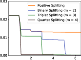
Loss	Loss
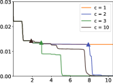
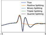
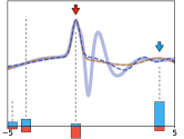
Iterations $(\times 10^{4})$	Iterations $(\times 10^{4})$
(a)	(b)	(c)	(d)

Figure 2: Results on a one-dimensional RBF network. (a) Loss curve of different splitting methods when $c=3$. (b) Loss curves of signed binary splittings ($m=2$) with different values of $c$. Note that $c=1$ reduces to positive splitting. The triangle markers indicate the first time when S2D and S3D give different splitting results. (c) The curve fitted by different splitting methods when the network grow into 5 neurons. (d) The centers of the RBF neurons (indicated by the bar centers) of the curve learned when applying signed binary splittings ($m=2$) for 4 steps, and their corresponding maximum and minimum eigenvalues (the blue and red bars). The blue and red arrows indicate the location of splitting according to the maximum and minimum eigenvalues, respectively, and the blue and orange dashed lines are the corresponding curves of binary splittings and positive splittings $(m=2)$ we obtained after the splittings.

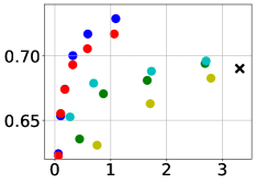
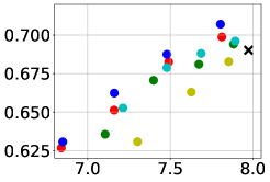
Test Accuracy	Test Accuracy		Test Accuracy
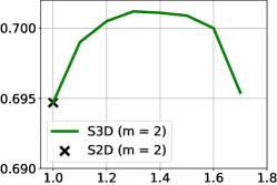
(a) # Params (M)	(b) Log10 (FLOPs)		(c) Value of c

Figure 3: Results of MobileNetV1 on CIFAR-100. (a) Testing accuracy v.s. the number of parameters of the models learned by S3D with binary splittings ($m=2$) and other baselines. (b) Results in the energy-aware setting by S3D with binary splittings ($m=2$) and other baselines. (c) Results of S2D and S3D ($m=2$) when $c$ varies in the same setting as that in (a) at the $5$th spitting step.

Results on CIFAR-100

We apply S3D to grow DNNs for the image classification task. We test our method on MobileNetV1 [16] on CIFAR-100 and compare our S3D with S2D [19] as well as other pruning baselines, including L1 Pruning [20], Bn Pruning [20] and MorphNet [13]. We also apply our algorithm in an energy-aware setting discussed in Wang et al. [33], which decides the best neurons to split by formulating a knapsack problem to best trade-off the splitting gain and energy cost; see Wang et al. [33] for the details. To speedup the eigen-computation in S3D and S2D, we use the fast gradient-based eigen-approximation algorithm in [33] (see Appendix E.3). Our results show that our algorithm outperforms prior arts with higher accuracy and lower cost in terms of both model parameter numbers and FLOPs. See more experiment detail in Appendix D.2

Figure 3 (a) and (b) show that our S3D algorithm outperforms all the baselines in both the standard-setting and the energy-aware setting of Wang et al. [33]. Table 2 reports the testing accuracy, parameter size and FLOPs of the learned models. We can see that our method achieves significantly higher accuracy as well as lower parameter sizes and FLOPs. We study the relation between testing accuracy and the hyper-parameter $c$ in Figure 3 (c), at the 5th splitting step in Figure 3 (a) (note that $c=1.0$ reduces to S2D). We can see that $c\approx 1.3$ is optimal in this case.

Method	Accuracy	# Param (M)	# Flops (M)
Full Size Baseline	69.04	3.31	94.13
L1 [20]	69.41	2.69	76.34
Bn [20]	69.61	2.71	78.15
MorphNet [13]	68.27	2.79	71.63
S2D-5 [19]	69.69	0.31	79.94
S3D-5	70.19	0.30	73.69

Table 1: Comparison of different methods when the testing accuracy is around 69%. S2D-5 and S3D-5 represent applying S2D and S3D $(m=2)$ for 5 splitting steps, respectively.

Model	MACs (G)	Top-1	Top-5
MobileNetV1 (1.0x)	0.569	72.93	91.14
S2D-4	0.561	73.96	91.49
S3D-4	0.558	74.12	91.50
MobileNetV1 (0.75x)	0.317	70.25	89.49
AMC [15]	0.301	70.50	89.30
S2D-3	0.292	71.47	89.67
S3D-3	0.291	71.61	89.83
MobileNetV1 (0.5x)	0.150	65.20	86.34
S2D-2	0.140	68.26	87.93
S3D-2	0.140	68.72	88.19
S2D-1	0.082	64.06	85.30
S3D-1	0.082	64.37	85.49
Seed	0.059	59.20	81.82

Table 2: Results of ImageNet classification using MobileNetV1. S2D-$k$ and S3D-$k$ denote we split the network $k$ times using S2D and S3D ($m=2$), respectively.

Model	Acc.	Forward time (ms)	# Param (M)
PointNet [25]	89.2	32.19	2.85
PointNet++ [26]	90.7	331.4	0.86
DGCNN (1.0x)	92.6	60.12	1.81
DGCNN (0.75x)	92.4	48.06	1.64
DGCNN (0.5x)	92.3	38.90	1.52
DGCNN-S2D-4	92.7	42.83	1.52
DGCNN-S3D-4	92.9	42.06	1.51

Table 3: Results on the ModelNet40 classification task. DGCNN-S2D-4 and DGCNN-S3D-4 denote applying S2D and S3D ($m=2$) for 4 splitting steps, respetively.

Results on ImageNet

We apply our method in ImageNet classification task. We follow the setting of [33], using their energy-aware neuron selection criterion and fast gradient-based eigen-approximation. We also compare our methods with AMC [15] , full MobileNetV1 and MobileNetV1 with $0.75\times$, $0.5\times$ width multipliers on each layers. We find that our S3D achieves higher Top-1 and Top-5 accuracy than other methods with comparable multiply-and-accumulate operations (MACs). See details of setting in Appendix D.3. Table 2 shows that our S3D obtains better Top-1 and Top-5 accuracy compared with the S2D in Wang et al. [33] and other baselines with the same or smaller MACs. We also visualize the filters after splitting on ImageNet; see Appendix D.4.

Results on Point Cloud Classification

We consider point cloud classification with Dynamic graph convolution neural network (DGCNN) [34]. DGCNN one of the best networks for point cloud, but tends to be expensive in both speed and space, because it involves K-nearest-neighbour (KNN) operators for aggregating neighboring features on the graph. We apply S3D to search better DGCNN structures with smaller sizes, hence significantly improving the space and time efficiency. Following the experiment in Wang et al. [34], we choose ModelNet40 as our dataset. See details in Appendix D.5. Table 3 shows the result compared with PointNet [25], PointNet++ [26] and DGCNN with different multiplier on its EgdConv layers. We compare the accuracy as well as model size and time cost for forward processing. For forward processing time, we test it on a single NVIDIA RTX 2080Ti with a batch size of 16. We can see that our S3D algorithm obtains networks with the highest accuracy among all the methods, with a faster forward processing speed than DGCNN ($0.75\times$) and a smaller model size than DGCNN ($0.5\times$).

4 Related Works

Neural Architecture Search (NAS) has been traditionally framed as a discrete combinatorial optimization and solved based on black-box optimization methods such as reinforcement learning [e.g. 39, 40], evolutionary/genetic algorithms [e.g., 31, 27], or continuous relaxation followed with gradient descent [e.g., 18, 38]. These methods need to search in a large model space with expensive evaluation cost, and can be computationally expensive or easily stucked at local optima. Techniques such as weight-sharing [e.g. 24, 5, 2] and low fidelity estimates [e.g., 40, 10, 28] have been developed to alleviate the cost problem in NAS; see e.g., Elsken et al. [9], Wistuba et al. [36] for recent surveys of NAS. In comparison, splitting steepest descent is based on a significantly different functional steepest view that leverages the fundamental topological information of deep neural architectures to enable more efficient search, ensuring both rigorous theoretical guarantees and superior practical performance.

The idea of progressively growing neural networks has been considered by researchers in various communities from different angles. However, most existing methods are based on heuristic ideas. For example, Wynne-Jones [37] proposed a heuristic method to split neurons based on the eigen-directions of covariance matrix of the gradient. See e.g., Ghosh & Tumer [12], Utgoff & Precup [32] for surveys of similar ideas in the classical literature.

Recently, Chen et al. [6] proposed a method called Net2Net for knowledge transferring which grows a well-trained network by splitting randomly picked neurons along random directions. Our optimal splitting strategies can be directly adapted to improve Net2Net. Going beyond node splitting, more general operators that grow networks while preserving the function represented by the networks, referred to as network morphism, have been studied and exploited in a series of recent works [e.g., 6, 35, 4, 8].

A more principled progressive training approach for neural networks can be derived using Frank-Wolfe [e.g., 29, 3, 1], which yields greedy algorithms that iteratively add optimal new neurons while keeping the previous neurons fixed. Although rigorous convergence rate can be established for these methods [e.g., 1], they are not practically applicable because adding each new neuron requires to solve an intractable non-convex global optimization problem. In contrast, the splitting steepest descent approach is fully computationally tractable, because the search of the optimal node splitting schemes amounts to an tractable eigen-decomposition problem (albeit being non-convex). The original S2D in Liu et al. [19] did not provide a convergence guarantee, because the algorithm gets stuck when the splitting matrices become positive definite. By using signed splittings, our S3D can escape more local optima, ensuring both strong theoretical guarantees and better empirical performance.

An alternative approach for learning small and energy-efficient networks is to prune large pre-trained neural networks to obtain compact sub-network structures [e.g., 14, 17, 20, 21, 11]. As shown in our experiments and Liu et al. [19], Wang et al. [33], the splitting approach can outperform existing pruning methods, without requiring the overhead of pre-traininging large models. A promising future direction is to design algorithms that adaptively combine splitting with pruning to achieve better results.

5 Conclusion

In this work, we develop an extension of the splitting steepest descent framework to avoid the local optima by introducing signed splittings. Our S3D can learn small and accurate networks in challenging cases. For future work, we will develop further speed up of S3D and explore more flexible ways for optimizing network architectures going beyond neuron splitting.

Appendix A Derivation of Optimal Splitting Schemes with Negative Weights

Lemma A.1.

Let $(\boldsymbol{\delta}^{*},\boldsymbol{w}^{*})$ be an optimal solution of (6). Then $\delta_{i}^{*}$ must be an eigen-vector of $S(\theta)$ unless $w_{i}^{*}=0$ or $\delta_{i}^{*}=0$.

Proof.

Write $S=S(\theta)$ for simplicity. With fixed weights $\boldsymbol{w}$, the optimization w.r.t. $\boldsymbol{\delta}$ is

$$\min_{\boldsymbol{\delta}}\sum_{i=1}^{m}w_{i}\delta_{i}^{\top}S\delta_{i}\leavevmode\nobreak\ \leavevmode\nobreak\ \leavevmode\nobreak\ s.t.\leavevmode\nobreak\ \leavevmode\nobreak\ \leavevmode\nobreak\ \left\lVert\sum_{i=1}^{m}w_{i}\delta_{i}\right\rVert=0,\leavevmode\nobreak\ \leavevmode\nobreak\ \left\lVert\delta_{i}\right\rVert=1.$$

By KKT condition, the optimal solution must satisfy

$$w_{i}^{*}S\delta_{i}^{*}-\lambda_{1}w_{i}^{*}\bar{\delta}^{*}-\lambda_{2}^{*}\delta_{i}=0$$

$$\bar{\delta}^{*}:=\sum_{i=1}^{m}w_{i}^{*}\delta_{i}^{*}=0,$$

where $\lambda_{1}$ and $\lambda_{2}$ are two Lagrangian multipliers. Canceling out $\bar{\delta}^{*}$ gives

$$w_{i}^{*}S\delta_{i}^{*}-\lambda_{2}\delta_{i}^{*}=0.$$

Therefore, if $w_{i}^{*}\neq 0$ and $\delta_{i}\neq 0$, then $\delta_{i}^{*}$ must be the eigen-vector of $S$ with eigen-value $\lambda_{2}/w_{i}^{*}$. ∎

A.1 Derivation of Optimal Binary Splittings ($m=2$)

Theorem A.2.

1) Consider the optimization in (6) with $m=2$ and $c\geq 1$. Then the optimal solution must satisfy

$$\delta_{1}=r_{1}v,\leavevmode\nobreak\ \leavevmode\nobreak\ \leavevmode\nobreak\ \leavevmode\nobreak\ \delta_{2}=r_{2}v,$$

where $v$ is an eigen-vector of $S(\theta)$ and $r_{1},r_{2}\in\mathbb{R}^{2}$ are two scalars.

2) In this case, the optimization reduces to

$$\begin{split}G_{2}^{-c}:=\min_{\boldsymbol{w},r,v}(w_{1}r_{1}^{2}&+w_{2}r_{2}^{2})\times\lambda\\ s.t.\leavevmode\nobreak\ \leavevmode\nobreak\ \leavevmode\nobreak\ &w_{1}+w_{2}=1\\ &w_{1}r_{1}+w_{2}r_{2}=0\\ &|w_{1}|+|w_{2}|\leq c\\ &|r_{1}|,|r_{2}|\leq 1\\ &\text{$\lambda$ is an eigen-value of $S(\theta)$}.\end{split}$$ (15)

3) The optimal value above is

$$G_{2}^{-c}=\min\left(\lambda_{\min},\leavevmode\nobreak\ \leavevmode\nobreak\ -\frac{c-1}{c+1}\lambda_{\max},\leavevmode\nobreak\ \leavevmode\nobreak\ 0\right).$$ (16)

If $-\frac{c-1}{c+1}\lambda_{\max}<\min(\lambda_{\min},0)$, the optimal solution is achieved by

$$w_{1}=-\frac{c-1}{2},\leavevmode\nobreak\ \leavevmode\nobreak\ \leavevmode\nobreak\ \leavevmode\nobreak\ \delta_{1}=v_{\max}, w_{2}=\frac{c+1}{2},\leavevmode\nobreak\ \leavevmode\nobreak\ \leavevmode\nobreak\ \leavevmode\nobreak\ \delta_{2}=\frac{c-1}{c+1}v_{\max}.$$

If $\lambda_{\min}<\min(-\frac{c-1}{c+1}\lambda_{\max},0)$ the optimal solution is achieved by

$$w_{1}=\frac{1}{2},\leavevmode\nobreak\ \leavevmode\nobreak\ \leavevmode\nobreak\ \leavevmode\nobreak\ \delta_{1}=v_{\min}, w_{2}=\frac{1}{2},\leavevmode\nobreak\ \leavevmode\nobreak\ \leavevmode\nobreak\ \leavevmode\nobreak\ \delta_{2}=-v_{\min}.$$

If $0\leq\min(\lambda_{\min},-\frac{c-1}{c+1}\lambda_{\max})$, and hence $\lambda_{\min}=\lambda_{\max}=0$, the optimal solution is achieved by no splitting: $\delta_{1}=\delta_{2}=0.$

Proof.

1) The form of $\delta_{1}=r_{1}v$ and $\delta_{2}=r_{2}v$ is immediately implied by the constraint $w_{1}\delta_{1}+w_{2}\delta_{2}=0$. By Lemma A.1, $v$ must be an eigen-vector of $S(\theta)$.

2) Plugging $\delta_{1}=r_{1}v$ and $\delta_{2}=r_{2}v$ into (6) directly implies (15).

3) Following (15), we seek to minimize the product of $t(\boldsymbol{w},r):=w_{1}r_{1}^{2}+w_{2}r_{2}^{2}$ and $\lambda$. If $\lambda\geq 0$, we need to minimize $t(\boldsymbol{w},r)$, while if $\lambda\leq 0$, we need to maximize $t(\boldsymbol{w},r)$. Lemma A.3 and A.4 below show that the minimum and maximum values of $t(\boldsymbol{w},r)$ equal $-\frac{c-1}{c+1}$ and $1$, respectively. Because the range of $\lambda$ is $[\lambda_{\min},\lambda_{\max}]$, we can write

$$G_{2}^{-c} =\min_{t,v}\left\{t\times\lambda\colon\leavevmode\nobreak\ \leavevmode\nobreak\ \leavevmode\nobreak\ -\frac{c-1}{c+1}\leq t\leq 1,\leavevmode\nobreak\ \leavevmode\nobreak\ \leavevmode\nobreak\ \lambda_{\min}\leq\lambda\leq\lambda_{\max}\right\}$$

$$=\min\left(\lambda_{\min},\leavevmode\nobreak\ \leavevmode\nobreak\ -\frac{c-1}{c+1}\lambda_{\max}\right).$$

From $\lambda_{\min}\leq\lambda_{\max}$, we can easily see that $G_{2}^{-c}\leq 0$, and hence the form above is equivalent to the result in Theorem 2.1. The corresponding optimal solutions follow Lemma A.3 and A.4 below, which describe the values of $(w_{1},w_{2},r_{1},r_{2})$ to minimize and maximize $w_{1}r_{1}^{2}+w_{2}r_{2}^{2}$, respectively. ∎

Lemma A.3.

Consider the following optimization with $c\geq 1$:

$$\begin{split}R_{2}^{\min}:=\min_{(\boldsymbol{w},r)\in\mathbb{R}^{4}}w_{1}r_{1}^{2}&+w_{2}r_{2}^{2}\\ \leavevmode\nobreak\ \leavevmode\nobreak\ \leavevmode\nobreak\ \leavevmode\nobreak\ s.t.\leavevmode\nobreak\ \leavevmode\nobreak\ \leavevmode\nobreak\ &w_{1}+w_{2}=1\\ &w_{1}r_{1}+w_{2}r_{2}=0\\ &|w_{1}|+|w_{2}|\leq c\\ &|r_{1}|,|r_{2}|\leq 1.\end{split}$$ (17)

Then we have $R_{2}^{\min}=-\frac{c-1}{c+1}$ and the optimal solution is achieved by the following scheme:

$$\begin{split}&w_{1}=-\frac{c-1}{2},\leavevmode\nobreak\ \leavevmode\nobreak\ \leavevmode\nobreak\ \leavevmode\nobreak\ r_{1}=1\\ &w_{2}=\frac{c+1}{2},\leavevmode\nobreak\ \leavevmode\nobreak\ \leavevmode\nobreak\ \leavevmode\nobreak\ r_{2}=\frac{c-1}{c+1}.\end{split}$$ (18)

Proof.

Case 1 ($w_{2}\leq 0$, $w_{1}\geq 1$)   Assume $w_{2}=-a$. We have $w_{1}=1+a>1$.

$$\min_{a,r_{1},r_{2}}(1+a)r_{1}^{2} -ar_{2}^{2}$$

$$\leavevmode\nobreak\ \leavevmode\nobreak\ \leavevmode\nobreak\ \leavevmode\nobreak\ s.t.\leavevmode\nobreak\ \leavevmode\nobreak\ \leavevmode\nobreak\ (1+a)r_{1}=ar_{2}$$

$$a\leq\frac{c-1}{2}$$

$$|r_{1}|,|r_{2}|\leq 1.$$

Eliminating $r_{1}$, we have

$$\min_{a,r_{2}}\left(-\frac{a}{1+a}\right)r_{2}^{2}\leavevmode\nobreak\ \leavevmode\nobreak\ \leavevmode\nobreak\ \leavevmode\nobreak\ \leavevmode\nobreak\ s.t.\leavevmode\nobreak\ \leavevmode\nobreak\ \leavevmode\nobreak\ \leavevmode\nobreak\ \leavevmode\nobreak\ a\leq\frac{c-1}{2},\leavevmode\nobreak\ \leavevmode\nobreak\ \leavevmode\nobreak\ \leavevmode\nobreak\ \leavevmode\nobreak\ |r_{2}|\leq 1.$$

The optimal solution is $r_{2}=1$ or $-1$, and $a=\frac{c-1}{2}$, for which we achieve a minimum value of $w_{1}r_{1}^{2}+w_{2}r_{2}^{2}=-\frac{c-1}{c+1}$.

Case 2 ($w_{1}\geq 0$, $w_{2}\geq 0$)   This case is obviously sub-optimal since we have $w_{1}r_{1}^{2}+w_{2}r_{2}^{2}\geq 0\geq-\frac{c-1}{c+1}$ in this case.

Overall, the minimum value is $-\frac{c-1}{c+1}$. This completes the proof. ∎

Lemma A.4.

Consider the following optimization with $c\geq 1$:

$$\begin{split}R_{2}^{\max}:=\max_{(\boldsymbol{w},r)\in\mathbb{R}^{4}}w_{1}r_{1}^{2}&+w_{2}r_{2}^{2}\\ \leavevmode\nobreak\ \leavevmode\nobreak\ \leavevmode\nobreak\ \leavevmode\nobreak\ s.t.\leavevmode\nobreak\ \leavevmode\nobreak\ \leavevmode\nobreak\ &w_{1}+w_{2}=1\\ &w_{1}r_{1}+w_{2}r_{2}=0\\ &|w_{1}|+|w_{2}|\leq c\\ &|r_{1}|,|r_{2}|\leq 1.\end{split}$$ (19)

Then we have $R_{2}^{\max}=1$, which is achieved by the following scheme:

$$\begin{split}&w_{1}=\frac{1}{2},\leavevmode\nobreak\ \leavevmode\nobreak\ \leavevmode\nobreak\ \leavevmode\nobreak\ r_{1}=1\\ &w_{2}=\frac{1}{2},\leavevmode\nobreak\ \leavevmode\nobreak\ \leavevmode\nobreak\ \leavevmode\nobreak\ r_{2}=-1.\end{split}$$ (20)

Proof.

It is easy to see that $R_{2}^{\max}\leq 1$. On the other hand, this bound is achieved by the scheme in (20). ∎

A.2 Derivation of Triplet Splittings ($m=3$)

Theorem A.5.

Consider the optimization in (6) with $m=3$ and $c\geq 1$.

1) The optimal solution of (6) must satisfy

$$\delta_{i}=\sum_{\ell=1}^{d_{\lambda}}r_{i,\ell}v_{\ell},$$

where $\{v_{\ell}\colon i=1,\ldots,{d_{\lambda}}\}$ is a set of $d_{\lambda}$ orthonormal eigen-vectors of $S(\theta)$ that share the same eigenvalue $\lambda$, and $\{r_{i,\ell}\}_{i,\ell}$ is a set of coefficients.

2) Write $r_{i}=[r_{i,1},\ldots,r_{r,d_{\lambda}}]\in\mathbb{R}^{d_{\lambda}}$ for $i=1,2,3$. The optimization in (6) is equivalent to

$$\begin{split}G_{3}^{-c}:=\min_{\boldsymbol{w},\boldsymbol{r},\lambda}(w_{1}\left\lVert r_{1}\right\rVert^{2}&+w_{2}\left\lVert r_{2}\right\rVert^{2}+w_{3}\left\lVert r_{3}\right\rVert^{2})\times\lambda\\ s.t.\leavevmode\nobreak\ \leavevmode\nobreak\ \leavevmode\nobreak\ &w_{1}+w_{2}+w_{3}=1\\ &w_{1}r_{1}+w_{2}r_{2}+w_{3}r_{3}=0\\ &|w_{1}|+|w_{2}|+|w_{3}|\leq c\\ &\left\lVert r_{1}\right\rVert,\left\lVert r_{2}\right\rVert,\left\lVert r_{3}\right\rVert\leq 1\\ &\text{$\lambda$ is an eigen-value of $S(\theta)$ with $d_{\lambda}$ orthogonal eigen-vectors}.\end{split}$$ (21)

3) The optimal value above is

$$G_{3}^{-c}=\min\left(\frac{c+1}{2}\lambda_{\min},\leavevmode\nobreak\ \leavevmode\nobreak\ -\frac{c-1}{2}\lambda_{\max},\leavevmode\nobreak\ \leavevmode\nobreak\ 0\right).$$ (22)

If $-\frac{c-1}{2}\lambda_{\max}<\frac{c+1}{2}\min(\lambda_{\min},0)$, the optimal solution is achieved by

$$\left(w_{1}=-\frac{c-1}{4},\leavevmode\nobreak\ \leavevmode\nobreak\ \leavevmode\nobreak\ \leavevmode\nobreak\ \delta_{1}=v_{\max}\right), \left(w_{2}=-\frac{c-1}{4},\leavevmode\nobreak\ \leavevmode\nobreak\ \leavevmode\nobreak\ \leavevmode\nobreak\ \delta_{2}=-v_{\max}\right), \left(w_{3}=\frac{c+1}{2},\leavevmode\nobreak\ \leavevmode\nobreak\ \leavevmode\nobreak\ \leavevmode\nobreak\ \delta_{3}=0\right).$$

If $\frac{c+1}{2}\lambda_{\min}<-\frac{c-1}{2}\max(\lambda_{\max},0)$

the optimal solution is achieved by

$$\left(w_{1}=\frac{c+1}{4},\leavevmode\nobreak\ \leavevmode\nobreak\ \leavevmode\nobreak\ \leavevmode\nobreak\ \delta_{1}=v_{\min}\right), \left(w_{2}=\frac{c+1}{4},\leavevmode\nobreak\ \leavevmode\nobreak\ \leavevmode\nobreak\ \leavevmode\nobreak\ \delta_{2}=-v_{\min}\right), \left(w_{3}=-\frac{c-1}{2},\leavevmode\nobreak\ \leavevmode\nobreak\ \leavevmode\nobreak\ \leavevmode\nobreak\ \delta_{3}=0\right).$$

If $0\leq\min\left(\frac{c+1}{2}\lambda_{\min},\leavevmode\nobreak\ -\frac{c-1}{2}\lambda_{\max}\right)$, and hence $\lambda_{\min}=\lambda_{\max}=0$, the optimal solution can be achieved by no splitting: $\delta_{1}=\delta_{2}=\delta_{3}=0$.

Proof.

1-2) Following Lemma A.1, the optimal $\delta_{1},\delta_{2},\delta_{3}$ are eigen-vectors of $S(\theta)$. Because eigen-vectors associated with different eigen-values are linearly independent, we have that $\delta_{1},\delta_{2},\delta_{3}$ must share the same eigen-value (denoted by $\lambda$) due to the constraint $w_{1}\delta_{1}+w_{2}\delta_{2}+w_{3}\delta_{3}=0$. Assume $\lambda$ is associated with $d_{\lambda}$ orthonormal eigen-vectors $\{v_{\ell}\}_{\ell=1}^{d_{\lambda}}$. Then we can write $\delta_{i}=\sum_{\ell}r_{i,\ell}v_{\ell}$ for $i=1,2,3$, for which $\left\lVert\delta_{i}\right\rVert=\left\lVert r_{i}\right\rVert$ and $\delta_{i}^{\top}S(\theta)\delta_{i}=\lambda\left\lVert r_{i}\right\rVert^{2}$. It is then easy to reduce (6) to (21). 3) Following Lemma A.6 and A.7, the value of $w_{1}\left\lVert r_{1}\right\rVert^{2}+w_{2}\left\lVert r_{2}\right\rVert^{2}+w_{3}\left\lVert r_{3}\right\rVert^{2}$ in (21) can range from $-\frac{c-1}{2}$ to $\frac{c+1}{2}$, for any positive integer $d_{\lambda}$. In addition, the range of the eigen-value $\lambda$ is $[\lambda_{\min},\lambda_{\max}]$. Therefore, we can write

$$G_{3}^{-c} =\min_{t,v}\left\{t\times\lambda\colon\leavevmode\nobreak\ \leavevmode\nobreak\ \leavevmode\nobreak\ -\frac{c-1}{2}\leq t\leq\frac{c+1}{2},\leavevmode\nobreak\ \leavevmode\nobreak\ \leavevmode\nobreak\ \lambda_{\min}\leq\lambda\leq\lambda_{\max}\right\}$$

$$=\min\left(-\frac{c-1}{2}\lambda_{\max},\leavevmode\nobreak\ \leavevmode\nobreak\ \leavevmode\nobreak\ \frac{c+1}{2}\lambda_{\min}\right).$$

Because $\lambda_{\min}\leq\lambda_{\max}$, we have $G_{3}^{-c}\leq 0$ and hence the result above is equivalent to the form in (22). The corresponding optimal solutions follow Lemma A.6 and A.7.

∎

Lemma A.6.

For any $c\geq 1$ and any positive integer $d_{r}$, define

$$\begin{split}R_{3,c,d_{\lambda}}^{\max}=\max_{\boldsymbol{w}\in\mathbb{R}^{3},r\in\mathbb{R}^{3\times d_{\lambda}}}(w_{1}\left\lVert r_{1}\right\rVert^{2}&+w_{2}\left\lVert r_{2}\right\rVert^{2}+w_{3}\left\lVert r_{3}\right\rVert^{2})\\ s.t.\leavevmode\nobreak\ \leavevmode\nobreak\ \leavevmode\nobreak\ &w_{1}+w_{2}+w_{3}=1\\ &|w_{1}|+|w_{2}|+|w_{3}|\leq c\\ &w_{1}r_{1}+w_{2}r_{2}+w_{3}r_{3}=0,\leavevmode\nobreak\ \leavevmode\nobreak\ \leavevmode\nobreak\ \forall\ell\\ &\left\lVert r_{i}\right\rVert\leq 1\leavevmode\nobreak\ \leavevmode\nobreak\ \leavevmode\nobreak\ \forall i=1,2,3.\end{split}$$ (23)

Then we have $R_{3,c,d_{\lambda}}^{\max}=\frac{c+1}{2}$ and the optimum is achieved by

$$\left(w_{1}=\frac{c+1}{4},\leavevmode\nobreak\ \leavevmode\nobreak\ \leavevmode\nobreak\ r_{1}=e\right) \left(w_{2}=\frac{c+1}{4},\leavevmode\nobreak\ \leavevmode\nobreak\ \leavevmode\nobreak\ r_{2}=-e\right) \left(w_{3}=-\frac{c-1}{2},\leavevmode\nobreak\ \leavevmode\nobreak\ \leavevmode\nobreak\ r_{3}=\boldsymbol{0}\right),$$ (24)

where $e$ is any vector whose norm equals one, that is, $\left\lVert e\right\rVert=1$.

Proof.

First, it is easy that verify that $R_{3,c,d_{\lambda}}^{\max}\geq\frac{c+1}{2}$ by taking the solution in (24). We just need to show that $R_{3,c,d_{\lambda}}^{\max}\leq\frac{c+1}{2}$.

Define $w_{i}^{+}=\max(w_{i},0)=({w_{i}+|w_{i}|})/{2}$. From $w_{1}+w_{2}+w_{3}=1$ and $|w_{1}|+|w_{2}|+|w_{3}|\leq c$, we have

$$w_{1}^{+}+w_{2}^{+}+w_{3}^{+}=\frac{(w_{1}+|w_{1}|+w_{2}+|w_{2}|+w_{3}+|w_{3}|)}{2}\leq\frac{c+1}{2}.$$

Therefore, under the constraints in (23), we have

$$R_{3,c,d_{\lambda}}^{\max} =\max_{\boldsymbol{w},r}(w_{1}\left\lVert r_{1}\right\rVert^{2}+w_{2}\left\lVert r_{2}\right\rVert^{2}+w_{3}\left\lVert r_{3}\right\rVert^{2})$$

$$\leq\max_{\boldsymbol{w},r}(w_{1}^{+}\left\lVert r_{1}\right\rVert^{2}+w_{2}^{+}\left\lVert r_{2}\right\rVert^{2}+w_{3}^{+}\left\lVert r_{3}\right\rVert^{2})$$

$$\leq\max_{\boldsymbol{w},r}(w_{1}^{+}+w_{2}^{+}+w_{3}^{+})$$

$$\leq\frac{c+1}{2}.$$

∎

Lemma A.7.

For any $c\geq 1$ and any positive integer $d_{r}$, define

$$\begin{split}R_{3,c,d_{\lambda}}^{\min}=\min_{\boldsymbol{w}\in\mathbb{R}^{3},r\in\mathbb{R}^{3\times d_{\lambda}}}(w_{1}\left\lVert r_{1}\right\rVert^{2}&+w_{2}\left\lVert r_{2}\right\rVert^{2}+w_{3}\left\lVert r_{3}\right\rVert^{2})\\ s.t.\leavevmode\nobreak\ \leavevmode\nobreak\ \leavevmode\nobreak\ &w_{1}+w_{2}+w_{3}=1\\ &|w_{1}|+|w_{2}|+|w_{3}|\leq c\\ &w_{1}r_{1}+w_{2}r_{2}+w_{3}r_{3}=0,\leavevmode\nobreak\ \leavevmode\nobreak\ \leavevmode\nobreak\ \forall\ell\\ &\left\lVert r_{i}\right\rVert\leq 1\leavevmode\nobreak\ \leavevmode\nobreak\ \leavevmode\nobreak\ \forall i=1,2,3.\end{split}$$ (25)

Then we have $R_{3,c,d_{\lambda}}^{\min}=-\frac{c-1}{2}$ and the optimum is achieved by

$$\left(w_{1}=-\frac{c-1}{4},\leavevmode\nobreak\ \leavevmode\nobreak\ \leavevmode\nobreak\ r_{1}=e\right) \left(w_{2}=-\frac{c-1}{4},\leavevmode\nobreak\ \leavevmode\nobreak\ \leavevmode\nobreak\ r_{2}=-e\right) \left(w_{3}=\frac{c+1}{2},\leavevmode\nobreak\ \leavevmode\nobreak\ \leavevmode\nobreak\ r_{3}=\boldsymbol{0}\right),$$ (26)

where $e$ is any vector whose norm equals one, that is, $\left\lVert e\right\rVert=1$.

Proof.

First, it is easy that verify that $R_{3,c,d_{\lambda}}^{\min}\leq-\frac{c-1}{2}$ by taking the solution in (26). We just need to show that $R_{3,c,d_{\lambda}}^{\min}\geq-\frac{c-1}{2}$.

Define $w_{i}^{-}=\min(w_{i},0)=({w_{i}-|w_{i}|})/{2}$. From $w_{1}+w_{2}+w_{3}=1$ and $|w_{1}|+|w_{2}|+|w_{3}|\leq c$, we have

$$w_{1}^{-}+w_{2}^{-}+w_{3}^{-}=\frac{(w_{1}-|w_{1}|+w_{2}-|w_{2}|+w_{3}-|w_{3}|)}{2}\geq-\frac{c-1}{2}.$$

Therefore, under the constraints in (25), we have

$$R_{3,c,d_{\lambda}}^{\min} =\min_{\boldsymbol{w},r}(w_{1}\left\lVert r_{1}\right\rVert^{2}+w_{2}\left\lVert r_{2}\right\rVert^{2}+w_{3}\left\lVert r_{3}\right\rVert^{2})$$

$$\geq\min_{\boldsymbol{w},r}(w_{1}^{-}\left\lVert r_{1}\right\rVert^{2}+w_{2}^{-}\left\lVert r_{2}\right\rVert^{2}+w_{3}^{-}\left\lVert r_{3}\right\rVert^{2})$$

$$\geq\min_{\boldsymbol{w},r}(w_{1}^{-}+w_{2}^{-}+w_{3}^{-})$$

$$\geq-\frac{c-1}{2}.$$

∎

A.3 Derivation of the Optimal Quartet Splitting $(m=4)$

Theorem A.8.

Let $\lambda_{\min}$, $\lambda_{\max}$ be the smallest and largest eigenvalues of $S(\theta)$, respectively, and $\lambda_{\min}$, $\lambda_{\max}$ their corresponding eigen-vectors. For the optimization in (6), we have for any positive integer $m$ and $c\geq 1$,

$$G_{m}^{-c}\geq\frac{c+1}{2}\min(\lambda_{\min},0)+\frac{1-c}{2}\max(\lambda_{\max},0).$$

In addition, this lower bound is achieved by splitting the neuron to $m=4$ copies, with

$$\begin{split}w_{1}=w_{2}=\frac{c+1}{4},&\ \ \ \ \ \ w_{3}=w_{4}=\frac{1-c}{4}\\ \delta_{1}=-\delta_{2}=\mathbb{I}(\lambda_{\min}\leq 0)v_{\min},&\ \ \ \ \ \ \delta_{3}=-\delta_{4}=\mathbb{I}(\lambda_{\max}\geq 0)v_{\max},\end{split}$$ (27)

where $\mathbb{I}(\cdot)$ denotes the indicator function.

Proof.

Denote by $I_{\boldsymbol{w}}^{+}:=\{i\in[m]\colon w_{i}>0\}$ and $I_{\boldsymbol{w}}^{-}:=\{i\in[m]\colon w_{i}<0\}$ the index set of positive and negative weights, respectively. And $S_{\boldsymbol{w}}^{+}=\sum_{i\in I_{\boldsymbol{w}}^{+}}w_{i}$ the sum of the positive weights. We have $\sum_{i}|w_{i}|=2S_{\boldsymbol{w}}^{+}-1\leq c$, yielding $0\leq S_{\boldsymbol{w}}^{+}\leq(c+1)/2$.

Note that we have $\delta_{i}^{\top}S(\theta)\delta_{i}\in[\min(\lambda_{\min},0),\leavevmode\nobreak\ \max(\lambda_{\max},0)]$ for $\left\lVert\delta_{i}\right\rVert\leq 1$. we have

$$G_{m}^{-c} =\min\left\{\sum_{i\in I_{\boldsymbol{w}}^{+}}w_{i}\delta_{i}^{\top}S(\theta)\delta_{i}+\sum_{i\in I_{\boldsymbol{w}}^{-}}w_{i}\delta_{i}^{\top}S(\theta)\delta_{i}\right\}$$

$$\geq S_{\boldsymbol{w}}^{+}\min(\lambda_{\min},0)\leavevmode\nobreak\ +\leavevmode\nobreak\ (1-S_{\boldsymbol{w}}^{+})\max(\lambda_{\max},0)$$

$$\geq\frac{c+1}{2}\min(\lambda_{\min},0)+\frac{1-c}{2}\max(\lambda_{\max},0).$$

On the other hand, it is easy to verify that this bound is achieved by the solution in (27). This completes the proof. ∎

Appendix B Convergence Analysis

We provide a simple analysis of the convergence of the training loss of signed splitting steepest descent (Algorithm 1) on one-hidden-layer neural networks. We show that our algorithm allows us to achieve a training MSE loss of $\eta$ by splitting at most $\mathcal{O}((n/(d\eta))^{3/2})$ steps, starting from a single-neuron network, where $n$ is data size and $d$ the dimension of the input dimension.

To set up, consider splitting a one-hidden-layer network,

$$f(x;\leavevmode\nobreak\ \boldsymbol{\theta},\boldsymbol{w})=\sum_{i=1}^{m}w_{i}\sigma(\theta_{i}^{\top}x),$$ (28)

where $\sigma\colon\mathbb{R}\to\mathbb{R}$ is an uni-variate activation function. Each of the $m$ neurons can be the offspring of some earlier neuron, and will be split further. Consider a general loss of form

$$L(\boldsymbol{\theta},\boldsymbol{w})=\mathbb{E}_{x\sim\mathcal{D}_{n}}[\Phi(f(x;\boldsymbol{\theta},\boldsymbol{w}))].$$

The splitting matrix of the $i$-th neuron can be shown to be

$$S_{i}(\boldsymbol{\theta},\boldsymbol{w})=w_{i}\mathbb{E}_{x\sim\mathcal{D}_{n}}\left[\Phi^{\prime}(f(x;\leavevmode\nobreak\ \boldsymbol{\theta},\boldsymbol{w}))\sigma^{\prime\prime}(\theta_{i}^{\top}x)xx^{\top}\right].$$

For an empirical dataset $\mathcal{D}_{n}=\{x^{(\ell)}\}_{\ell=1}^{n}$, define

$$\textbf{X}=\left[\textbf{{Vec}}(x^{(1)}x^{(1)\top}),...,\textbf{{Vec}}(x^{(n)}x^{(n)\top})\right]\in\mathbb{R}^{d^{2}\times n}.$$

where $\textbf{{Vec}}(A)$ denotes the vectorization of matrix $A$.

We start with showing that the training loss can be controlled by the spectrum radius $\rho(S_{i}(\boldsymbol{\theta},\boldsymbol{w}))$ of the splitting matrix of any neuron. This allows us to establish provable bounds on the loss because $\rho(S_{i}(\boldsymbol{\theta},\boldsymbol{w}))$ is expected to be zero or small when the signed splitting descent converges.

Assumption B.1.

Consider the network in (28) with mean square loss $\Phi(f(x)):={\color[rgb]{0,0,0}\frac{1}{2}}(f(x)-y(x))^{2}$, where $y(x)$ denotes the label associated with $x$. Assume $\lambda_{\textbf{X}}:=\lambda_{\min}\left(\textbf{X}^{\top}\textbf{X}/d^{{2}}\right)>0$, and $|\sigma^{\prime\prime}(\theta_{i}^{\top}x^{(\ell)})|\geq h$ for $i\in[m]$ and $\ell\in[n]$. Assume $\left\lVert\nabla^{3}_{\boldsymbol{\theta}^{3}}L(\boldsymbol{\theta},\boldsymbol{w})\right\rVert_{\infty}\leq 6C$ for all the values of $\boldsymbol{\theta}$ and $\boldsymbol{w}$ reachable by our algorithm.

Remark

Notice that the assumption $\lambda_{\textbf{X}}>0$ requires that $d^{2}>0$, which holds for most computer vision dataset, e.g. , CIFAR and ImageNet.

Lemma B.2.

Under Assumption B.1, denote by $\rho({S_{i}}):=\max\left\{\left|\lambda_{\max}\left(S_{i}(\boldsymbol{\theta},\boldsymbol{w})\right)\right|,\left|\lambda_{\min}\left(S_{i}(\boldsymbol{\theta},\boldsymbol{w})\right)\right|\right\}$ the spectrum radius of $S_{i}(\boldsymbol{\theta},\boldsymbol{w})$, and $\alpha={n}/({dh^{2}\lambda_{\textbf{X}}})$. We have

$$\mathbb{E}_{x\sim\mathcal{D}_{n}}\left[(f(x;\boldsymbol{\theta},\boldsymbol{w})-y(x))^{2}\right]\leq\alpha{(\rho(S_{i})/w_{i})^{2}},\leavevmode\nobreak\ \leavevmode\nobreak\ \forall i\in[m].$$

Assumption B.3.

Assume Assumption B.1 holds. Let $\eta$ be any positive constant, and define $\rho_{0}:=(\eta/\alpha)^{1/2}=h(\lambda_{\textbf{X}}\eta d/n)^{1/2}$. Assume we apply Algorithm 1 to the neural network in (28), following the guidance below:

1) At each splitting step, we pick any neuron with $w_{i}^{2}\geq 1$ and $\rho(S_{i})\geq\rho_{0}$ and split it with the optimal splittings in Theorem 2.1-2.3 (with $m=2,3\text{\leavevmode\nobreak\ or\leavevmode\nobreak\ }4$). The algorithm stops when either $L(\boldsymbol{\theta},\boldsymbol{w})\leq\eta$, or such neurons can not be found.

2) Assume the step-size $\epsilon$ used in the splitting updates satisfies $\epsilon\leq\frac{1}{4C}\kappa_{m}\rho_{0}=\mathcal{O}((d\eta/n)^{1/2})$.

3) Assume we only update $\boldsymbol{\theta}$ during the parametric optimization phase while keeping $\boldsymbol{w}$ unchanged, and the parametric optimization does not deteriorate the loss.

Theorem B.4.

Assume we run Algorithm 1 with triplet or quartet splittings $(m=3\text{\leavevmode\nobreak\ or\leavevmode\nobreak\ }4)$ and $c\geq 3$, and Assumption B.3 holds. If we initialize the network with a single neuron that satisfies $w_{i}^{2}\geq 1$, then the algorithm achieves $L(\boldsymbol{\theta},\boldsymbol{w})\leq\eta$ with at most $T:=\left\lceil\beta\epsilon^{-2}\left(\frac{n}{d\eta}\right)^{1/2}\right\rceil$ iterations, where

$$\beta=4(\kappa_{3}h\sqrt{\lambda_{\textbf{X}}})^{-1}\max(L(\boldsymbol{\theta}_{0},\boldsymbol{w}_{0})-\eta,0).$$

In this case, we are able to obtain a neural network that achieves $L(\boldsymbol{\theta},\boldsymbol{w})\leq\eta$ with $2T+1$ neurons via triplet splitting, and $3T+1$ neurons via quartet splitting.

Since $\epsilon=\mathcal{O}((d\eta/n)^{1/2})$ by Assumption B.3, our result suggests that we can learn a neural network with $\mathcal{O}((n/(d\eta))^{3/2})$ neurons to achieve a loss no larger than $\eta$. Note that this is much smaller than the number of neurons required for over-parameterization-based analysis of standard gradient descent training of neural networks. For example, the analysis in Du et al. [7] requires $\mathcal{O}(n^{6})$ neurons, or $\mathcal{O}(n^{2}/d)$ in Oymak & Soltanolkotabi [22], much larger than what we need when $n$ is large.

Similar result can be established for binary splittings ($m=2$), but extra consideration is needed. The problem is that the positive binary splitting halves the output weight of the neurons at each splitting, which makes $w_{i}$ of all the neurons small and hence yields a loose bound in (B.2). This problem is sidestepped in Theorem B.4 for triplet and quartet splittings by taking $c\geq 3$ to ensure $(c+1)/4\geq 1$, so that there always exists at least one off-spring whose output weight is larger than 1 after the splitting. There are several different ways for addressing this issue for binary splittings. One simple approach is to initialize the network to have $T$ neurons with $w_{i}^{2}\geq 1$, so that there always exists neurons with $w_{i}^{2}\geq 1$ during the first $T$ iterations, and yields a neural network with $2T$ neurons at end. We provide a throughout discussion of this issue in the Appendix.

Appendix C Proof of Theoretical Analysis

C.1 Proof of Lemma B.2

Lemma B.2   Under Assumption B.1, denote by $\rho({S_{i}}):=\max\left\{\left|\lambda_{\max}\left(S_{i}(\boldsymbol{\theta},\boldsymbol{w})\right)\right|,\left|\lambda_{\min}\left(S_{i}(\boldsymbol{\theta},\boldsymbol{w})\right)\right|\right\}$ the spectrum radius of $S_{i}(\boldsymbol{\theta},\boldsymbol{w})$, and $\alpha={n}/({dh^{2}\lambda_{\textbf{X}}})$. We have

$$\mathbb{E}_{x\sim\mathcal{D}_{n}}\left[(f(x;\boldsymbol{\theta},\boldsymbol{w})-y(x))^{2}\right]\leq\alpha{(\rho(S_{i})/w_{i})^{2}},\leavevmode\nobreak\ \leavevmode\nobreak\ \forall i\in[m].$$

Proof.

We want to bound the mean square error using the spectrum radius of the splitting matrix. For the mean square loss, a derivation shows that the splitting matrix of the $i$-th neuron is

$$S_{i}=\frac{1}{n}\sum_{\ell=1}^{n}w_{i}e_{\ell}h_{i,\ell}\left(x^{(\ell)}x^{(\ell)\top}\right), e_{\ell}:=f(x^{(\ell)};\leavevmode\nobreak\ \boldsymbol{\theta},\boldsymbol{w})-y(x^{(\ell)}), h_{i,\ell}:=\sigma^{\prime\prime}(\theta_{i}^{\top}x^{(\ell)}).$$

Denote $\left\lVert\cdot\right\rVert_{F}$ as the Frobenius norm. We have

$$\left\lVert S_{i}\right\rVert_{F}=\left\lVert\textbf{{Vec}}(S_{i})\right\rVert_{2} =\frac{1}{n}\left\lVert\sum_{\ell=1}^{n}w_{i}e_{\ell}h_{i,\ell}\textbf{{Vec}}\left(x^{(\ell)}x^{(\ell)^{\top}}\right)\right\rVert_{2}$$

$$\geq d\sqrt{\lambda_{\textbf{X}}}\frac{1}{n}\sqrt{\sum_{\ell=1}^{n}(w_{i}e_{\ell}h_{i,\ell})^{2}}$$

$$\geq d\sqrt{\lambda_{\textbf{X}}}\frac{1}{n}|w_{i}|h\sqrt{\sum_{\ell=1}^{n}(e_{\ell})^{2}},\leavevmode\nobreak\ \leavevmode\nobreak\ \leavevmode\nobreak\ \leavevmode\nobreak\ \leavevmode\nobreak\ \leavevmode\nobreak\ \leavevmode\nobreak\ \text{{\color[rgb]{1,0,1}//because $|h_{i,\ell}|\geq h$, $\forall i,\ell$}}.$$

On the other hand,

$$\left\lVert S_{i}\right\rVert_{F}^{2}=\mathrm{tr}(S_{i}^{2})\leq d\rho(S_{i}^{2})=d\rho(S_{i})^{2},$$

where $\rho(S_{i}^{2})=\rho(S_{i})^{2}$ holds because $S_{i}$ is a symmetric matrix. This gives

$$\mathbb{E}_{x\sim D_{n}}\left[(f(x;\boldsymbol{\theta},\boldsymbol{w})-y(x))^{2}\right]=\frac{1}{n}{\sum_{\ell=1}^{n}(e_{\ell})^{2}}\leq\frac{n\rho(S_{i})^{2}}{h^{2}d\lambda_{\textbf{X}}w_{i}^{2}}.$$

∎

C.2 Convergence Rate of Triplet and Quartet Splittings

Proof of Theorem B.4.

First, when $c\geq 3$, note that the triplet and quartet splittings always yield at least one off-spring whose weight’s absolute value is no smaller than 1 (because $(c+1)/2\geq(c+1)/4\geq 1$ when $c\geq 3$). Since there is at least one neuron satisfies $w_{i}^{2}\geq 1$ in the initialization, there always exist neurons with $w_{i}^{2}\geq 1$ throughout the algorithm.

If there exists a neuron $i$ such that $w_{i}^{2}\geq 1$ and $\rho(S_{i})\leq|w_{i}|(\eta/\alpha)^{1/2}$ within the first $T$ iterations of signed splitting, we readily have by Lemma B.2

$$L(\boldsymbol{\theta},\boldsymbol{w})\leq\alpha(\rho(S_{i})/w_{i})^{2}\leq\eta.$$

If this does not hold, then $\alpha(\rho(S_{i})/w_{i})^{2}\geq\eta$ holds for every neuron in the first $T$ iterations. This means that the neurons with $w_{i}^{2}\geq 1$ must have $\rho(S_{i})\geq(\eta/\alpha)^{1/2}$.

Let $(\boldsymbol{\theta}^{\prime},\boldsymbol{w}^{\prime})$ be the parameter and weights we obtained by applying an optimal triplet splitting on $(\boldsymbol{\theta},\boldsymbol{w})$. We have by the Taylor expansion in Theorem 2.2 and Theorem 2.4 of Liu et al. [19], we have

$$L(\boldsymbol{\theta}^{\prime},\boldsymbol{w}^{\prime}) \leq L(\boldsymbol{\theta},\boldsymbol{w})+\frac{\epsilon^{2}}{2}G_{m}^{-c}+C\epsilon^{3}$$

$$\leq L(\boldsymbol{\theta},\boldsymbol{w})-\frac{\epsilon^{2}}{2}\kappa_{3}\rho(S_{i})+C\epsilon^{3}$$

$$\leq L(\boldsymbol{\theta},\boldsymbol{w})-\frac{\epsilon^{2}}{2}\kappa_{3}({\eta/\alpha})^{1/2}+C\epsilon^{3}.$$

Therefore, through the first $T$ iterations of splitting descent, we have

$$L(\boldsymbol{\theta}_{T},\boldsymbol{w}_{T}) \leq L(\boldsymbol{\theta}_{0},\boldsymbol{w}_{0})-T\left(\frac{\epsilon^{2}}{2}\kappa_{3}({\eta/\alpha})^{1/2}-C\epsilon^{3}\right)$$

$$\leq L(\boldsymbol{\theta}_{0},\boldsymbol{w}_{0})-T\left(\frac{\epsilon^{2}}{4}\kappa_{3}({\eta/\alpha})^{1/2}\right)\leavevmode\nobreak\ \leavevmode\nobreak\ \leavevmode\nobreak\ \leavevmode\nobreak\ \leavevmode\nobreak\ \leavevmode\nobreak\ \leavevmode\nobreak\ \text{{\color[rgb]{1,0,1}//because we assume $\epsilon\leq\frac{1}{4C}\kappa_{3}(\eta/\alpha)^{1/2}$}}$$

$$\leq\eta.\leavevmode\nobreak\ \leavevmode\nobreak\ \leavevmode\nobreak\ \leavevmode\nobreak\ \leavevmode\nobreak\ \leavevmode\nobreak\ \leavevmode\nobreak\ \text{{\color[rgb]{1,0,1}//because we assume $T=\left\lceil 4\left(\epsilon^{2}\kappa_{3}(\eta/\alpha)^{1/2}\right)^{-1}(L(\boldsymbol{\theta}_{0},\boldsymbol{w}_{0})-\eta)\right\rceil$}}$$

This completes the proof. ∎

C.3 Convergence of Binary Splitting

Theorem C.1.

Assume we run Algorithm 1 with signed binary splittings $(m=2)$ and $c\geq 1$, and Assumption B.3 holds. Assume we initialize the network with $(\boldsymbol{\theta}_{0},\boldsymbol{w}_{0})$ with $m_{0}$ neurons such that there is at least

$$T:=\left\lceil\beta n^{1/2}d^{-1/2}\epsilon^{-2}\eta^{-1/2}\right\rceil$$

neurons satisfying $w_{i}^{2}\geq 1$, where $\beta=4(\kappa_{2}h^{2}\lambda_{\textbf{X}}^{2})^{-1}\max(L(\boldsymbol{\theta}_{0},\boldsymbol{w}_{0})-\eta,0)$.

Then the algorithm determines within at most $T$ iterations, and return a neural network that achieves $L(\boldsymbol{\theta},\boldsymbol{w})\leq\eta$ with $T+m_{0}$ neurons.

As shown in Lemma C.2, we require the initialization condition of Lemma C.2 in Theorem C.1 with $m_{0}=\mathcal{O}(n^{3/2}d^{-3/2}\eta^{-3/2})$, which implies that signed binary splitting can learn neural networks with $\mathcal{O}(n^{3/2}d^{-3/2}\eta^{-3/2})$ neurons to achieve $L(\boldsymbol{\theta},\boldsymbol{w})\leq\eta$.

Remark

Indeed, if the initialization condition in Lemma C.2 holds, Theorem C.1 can be generalized for triplet and quartet splitting easily for any $c>1$.

Proof of Theorem C.1.

First, because there are at least $T$ neurons with $w_{i}^{2}\geq 1$ and each splitting step splits only one such neurons, there must exist neurons with $w_{i}^{2}\geq 1$ throughout the first $T$ iterations.

If there exists a neuron $i$ such that $w_{i}^{2}\geq 1$ and $\rho(S_{i})\leq|w_{i}|(\eta/\alpha)^{1/2}$ within the first $T$ iterations of signed splitting, we readily have by Lemma B.2

$$L(\boldsymbol{\theta},\boldsymbol{w})\leq\alpha(\rho(S_{i})/w_{i})^{2}\leq\eta.$$

If this does not hold, then $\alpha(\rho(S_{i})/w_{i})^{2}\geq\eta$ holds for every neuron in the first $T$ iterations. This means that the neurons with $w_{i}^{2}\geq 1$ must have $\rho(S_{i})\geq(\eta/\alpha)^{1/2}$.

Let $(\boldsymbol{\theta}^{\prime},\boldsymbol{w}^{\prime})$ be the parameter and weights we obtained by applying an optimal trplet splitting on $(\boldsymbol{\theta},\boldsymbol{w})$. By the Taylor expansion in Theorem 2.2 and Theorem 2.4 of Liu et al. [19], we have

$$L(\boldsymbol{\theta}^{\prime},\boldsymbol{w}^{\prime}) \leq L(\boldsymbol{\theta},\boldsymbol{w})+\frac{\epsilon^{2}}{2}G_{2}^{-c}+C\epsilon^{3}$$

$$\leq L(\boldsymbol{\theta},\boldsymbol{w})-\frac{\epsilon^{2}}{2}\kappa_{2}\rho(S_{i})+C\epsilon^{3}$$

$$\leq L(\boldsymbol{\theta},\boldsymbol{w})-\frac{\epsilon^{2}}{2}\kappa_{2}({\eta/\alpha})^{1/2}+C\epsilon^{3}.$$

Therefore, through the first $T$ iterations of splitting descent, we have

$$L(\boldsymbol{\theta}_{T},\boldsymbol{w}_{T}) \leq L(\boldsymbol{\theta}_{0},\boldsymbol{w}_{0})-T\left(\frac{\epsilon^{2}}{2}\kappa_{2}({\eta/\alpha})^{1/2}-C\epsilon^{3}\right)$$

$$\leq L(\boldsymbol{\theta}_{0},\boldsymbol{w}_{0})-T\left(\frac{\epsilon^{2}}{4}\kappa_{2}({\eta/\alpha})^{1/2}\right)\leavevmode\nobreak\ \leavevmode\nobreak\ \leavevmode\nobreak\ \leavevmode\nobreak\ \leavevmode\nobreak\ \leavevmode\nobreak\ \leavevmode\nobreak\ \text{{\color[rgb]{1,0,1}//because we assume $\epsilon\leq\frac{1}{4C}\kappa_{3}(\eta/\alpha)^{1/2}$}}$$

$$\leq\eta.\leavevmode\nobreak\ \leavevmode\nobreak\ \leavevmode\nobreak\ \leavevmode\nobreak\ \leavevmode\nobreak\ \leavevmode\nobreak\ \leavevmode\nobreak\ \text{{\color[rgb]{1,0,1}//because we assume $T=\left\lceil 4\left(\epsilon^{2}\kappa_{3}(\eta/\alpha)^{1/2}\right)^{-1}(L(\boldsymbol{\theta}_{0},\boldsymbol{w}_{0})-\eta)\right\rceil$}}$$

This completes the proof. ∎

Lemma C.2.

Assume $\sigma(0)=0$, $\left\lVert\sigma\right\rVert_{\mathrm{Lip}}<\infty$, and $r_{\mathcal{D}_{n}}=\max_{(x,y)\sim\mathcal{D}_{n}}(\left\lVert x\right\rVert,|y|)<\infty$. Let $r$ be any positive constant and $\ell_{0}=r_{\mathcal{D}_{n}}(1+r\left\lVert\sigma\right\rVert_{\mathrm{Lip}})$.

If we initialize $(\boldsymbol{\theta}_{0},\boldsymbol{w})$ with $m_{0}:=\left\lceil\left(4\epsilon^{2}\kappa_{2}(\eta/\alpha)^{1/2}\right)^{-1}(\ell_{0}-\eta)\right\rceil$ neurons, such that $w_{i,0}^{2}=1$ and $\left\lVert\theta_{i}\right\rVert\leq\frac{r}{m_{0}}$, then there exists at least

$$T=m_{0}\geq\left\lceil\left(4\epsilon^{2}\kappa_{2}(\eta/\alpha)^{1/2}\right)^{-1}(L(\boldsymbol{\theta}_{0},\boldsymbol{w}_{0})-\eta)\right\rceil$$

neurons that satisfies $w_{i,0}^{2}\geq 1$.

Proof.

$$L(\boldsymbol{\theta}_{0},\boldsymbol{w}_{0}) =\mathbb{E}_{(x,y)\sim\mathcal{D}_{n}}\left[\left(y-\sum_{i=1}^{m_{0}}w_{i,0}\sigma(\theta_{i,0}^{\top}x)\right)^{2}\right]$$

$$\leq\mathbb{E}_{(x,y)\sim\mathcal{D}_{n}}\left[\left(|y|+m_{0}\left\lVert\sigma\right\rVert_{\mathrm{Lip}}\left\lVert\theta\right\rVert\left\lVert x\right\rVert\right)^{2}\right]$$

$$\leq r_{\mathcal{D}_{n}}(1+k\left\lVert\sigma\right\rVert_{\mathrm{Lip}})$$

$$=\ell_{0}.$$

This obviously concludes the result. ∎

Appendix D Experiment Detail

D.1 Toy RBF neural network

Following Liu et al. [19], we consider the following one-hidden-layer RBF neural network with one-dimensional inputs:

$$\!\!\!\!\!\!\!f(x)=\sum_{i=1}^{m}w_{i}\sigma(\theta_{i1}x+\theta_{i2}), \sigma(x)=\exp(-\frac{x^{2}}{2}),$$ (29)

where $x,w_{i}\in\mathbb{R}$ and $\theta_{i}=[\theta_{i1},\theta_{i2}]\in\mathbb{R}^{2}$ for $\forall i\in[m]$. We define an underlying true function by taking $m=15$ neurons and drawing $w_{i}$ and the elements of $\theta_{i}$ i.i.d. from $\mathcal{N}(0,3)$. We then simulate a dataset $\{x^{(\ell)},y^{(\ell)}\}_{\ell=1}^{1000}$ by drawing $x^{(\ell)}$ from $\mathrm{Uniform}([-5,5])$ and $y^{(\ell)}=f(x^{(\ell)})$.

Because different $m$ yields different numbers of new neurons at each splitting, we set the number of gradient descent iterations during the parametric update phase to be $(m-1)\times 10k$ for each $m\in\{2,3,4\}$, so that neural networks of the same size is trained with the same number of gradient descent iterations. We use Adam optimizer with learning rate 0.005 for parametric gradient descent in all the splitting methods.

D.2 CIFAR-100

We train MobileNetV1 starting from a small network with 32 filters in each layer. MobileNetV1 contains two type of layers: the depth-wise layer and the point-wise layer. We grow the network by splitting the filters in the point-wise layers following Algorithm 1. In parametric update phase, we train the network for 160 epochs with batch size 128. We use stochastic gradient descent with momentum 0.1, weight decay $10^{-4}$, and learning rate $0.1$. We apply a decay rate 0.1 on the learning rate when we reach 50$\%$ and 75$\%$ of the total training epochs. In the splitting phase, we set the splitting step size $\epsilon=0.01$, choose $c=1.3$, and split the top $35\%$ of the current filters at each splitting phase. Our experiments in the energy-aware setting follows Wang et al. [33] closely, by keeping their code unchanged expect replacing positive splitting schemes with binary signed splittings with $c=1.3$.

D.3 ImageNet

We test different methods on MobileNetV1 following the same setting in Wang et al. [33]: when we update parameters, we set the batch size to be 128 for each GPU and use 4 GPUs in total, we use stochastic gradient descent with the cosine learning rate scheduler and set the initial learning rate to be 0.2. We also use label-smoothing (0.1) and 5 epochs warm-up. When splitting the networks, we set the splitting step size $\epsilon=0.01$ and keep the number of MACs close to the MACs of S2D reported in Wang et al. [33].

D.4 Filter Visualization Result

We visualize the filters picked by S2D/S3D when splitting VGG19. We take the pre-trained VGG19 on ImageNet, and evaluate the splitting matrices of the filters in the last convolution layer on a randomly picked image. We then pick the filters with the largest or smallest $\lambda_{\min}$ or $\lambda_{\max}$ and visualize them before and after splitting. We use guided gradient back-propagation [30] as the visualization tool and apply a gray-scale on the output image to have a better visualization. During the splitting, we set the splitting step size $\epsilon=0.01$.

Figure 4 visualizes the filters on an image whose label is “bulldog” (see Appendix 5 for more examples). We see that the filters with large $\rho:=\max(|\lambda_{\min}|,|\lambda_{\max}|)$ tend to change significantly after splitting. In contrast, the filters with small $\rho$ tend to keep unchanged after splitting. This suggests that the spectrum radius $\rho$ provides a good estimation of the benefit of splitting. We further include three more visualization of the splitting of filters on ImageNet in Figure 5. All the cases show similar consistent patterns illustrated above.

\begin{overpic}[width=433.62pt]{figure/visualization/dog_vis_new2.pdf} \put(22.0,19.0){$\theta\pm\epsilon v_{\min}$} \put(22.0,16.0){$\lambda_{\min}\text{=-}0.5$} \put(33.5,19.0){$\theta\pm\epsilon v_{\max}$} \put(33.0,16.0){$\lambda_{\max}\text{=}22.1$} \par\put(41.7,19.0){$\theta\pm\epsilon v_{\min}$} \put(41.7,16.0){$\lambda_{\min}\text{=-}29.2$} \put(53.2,19.0){$\theta\pm\epsilon v_{\max}$} \put(53.2,16.0){$\lambda_{\max}\text{=}10^{\text{-7}}$} \par\put(61.3,19.0){$\theta\pm\epsilon v_{\min}$} \put(61.3,16.0){$\lambda_{\min}\text{=-}23.6$} \put(72.8,19.0){$\theta\pm\epsilon v_{\max}$} \put(72.8,16.0){$\lambda_{\max}\text{=}0.3$} \par\put(80.9,19.0){$\theta\pm\epsilon v_{\min}$} \put(80.9,16.0){$\lambda_{\min}\text{=-}10^{\text{-}8}$} \put(92.3,19.0){$\theta\pm\epsilon v_{\max}$} \put(92.0,16.0){$\lambda_{\max}\text{=}10^{\text{-}2}$} \par\put(5.0,-1.5){(a) Original Image} \put(25.0,-1.5){(b) Largest $\lambda_{\max}$} \put(45.0,-1.5){(c) Smallest $\lambda_{\min}$} \put(65.0,-1.5){(d) Smallest $G_{4}^{-c}$} \put(83.0,-1.5){(e) Smallest $\rho(S(\theta))$} \end{overpic}

Figure 4: Filter visualization result. The filters are visualized by guided backpropagation. The center figures in (b)-(d) are the visualization of the different filters before splitting. The four surrounding figures in each panel are the results we get after split the neurons with $\theta\leftarrow\theta\pm\epsilon v_{\min}$ (left) and $\theta\leftarrow\theta\pm\epsilon v_{\max}$ (right), respectively. The figures with colored dashed boxes are the cases with significant changes after splitting, whose corresponding eigen-values tend to be far away from zero comparing with the other cases.

\begin{overpic}[width=429.28616pt]{figure/visualization/hat_vis_new2.pdf} \put(21.0,17.3){$\theta\pm\epsilon v_{\min}$} \put(21.0,14.3){$\lambda_{\min}\text{=-}10^{\text{-7}}$} \put(32.5,17.3){$\theta\pm\epsilon v_{\max}$} \put(32.0,14.3){$\lambda_{\max}\text{=}17.4$} \par\put(41.1,17.3){$\theta\pm\epsilon v_{\min}$} \put(41.1,14.3){$\lambda_{\min}\text{=-}44.7$} \put(52.6,17.3){$\theta\pm\epsilon v_{\max}$} \put(52.6,14.3){$\lambda_{\max}\text{=}10^{\text{-7}}$} \par\put(61.0,17.3){$\theta\pm\epsilon v_{\min}$} \put(61.0,14.3){$\lambda_{\min}\text{=-}23.5$} \put(72.5,17.3){$\theta\pm\epsilon v_{\max}$} \put(72.5,14.3){$\lambda_{\max}\text{=}10^{\text{-7}}$} \par\put(80.9,17.3){$\theta\pm\epsilon v_{\min}$} \put(80.9,14.3){$\lambda_{\min}\text{=-}10^{\text{-}8}$} \put(92.3,17.3){$\theta\pm\epsilon v_{\max}$} \put(92.0,14.3){$\lambda_{\max}\text{=}0.3$} \par\par\end{overpic}
\begin{overpic}[width=433.62pt]{figure/visualization/snake_vis_new2.pdf} \put(22.0,19.0){$\theta\pm\epsilon v_{\min}$} \put(22.0,16.0){$\lambda_{\min}\text{=-}10^{\text{-2}}$} \put(33.5,19.0){$\theta\pm\epsilon v_{\max}$} \put(33.0,16.0){$\lambda_{\max}\text{=}12.5$} \par\put(41.7,19.0){$\theta\pm\epsilon v_{\min}$} \put(41.7,16.0){$\lambda_{\min}\text{=-}21.3$} \put(53.2,19.0){$\theta\pm\epsilon v_{\max}$} \put(53.2,16.0){$\lambda_{\max}\text{=}10^{\text{-7}}$} \par\put(61.3,19.0){$\theta\pm\epsilon v_{\min}$} \put(61.3,16.0){$\lambda_{\min}\text{=-}16.2$} \put(72.8,19.0){$\theta\pm\epsilon v_{\max}$} \put(72.8,16.0){$\lambda_{\max}\text{=}10^{\text{-7}}$} \par\put(80.9,19.0){$\theta\pm\epsilon v_{\min}$} \put(80.9,16.0){$\lambda_{\min}\text{=-}10^{\text{-}9}$} \put(92.3,19.0){$\theta\pm\epsilon v_{\max}$} \put(92.0,16.0){$\lambda_{\max}\text{=}10^{\text{-}4}$} \par\par\end{overpic}
\begin{overpic}[width=437.95381pt]{figure/visualization/bottle_vis_new2.pdf} \put(22.7,17.0){$\theta\pm\epsilon v_{\min}$} \put(22.7,14.0){$\lambda_{\min}\text{=-}10^{\text{-8}}$} \put(34.2,17.0){$\theta\pm\epsilon v_{\max}$} \put(33.7,14.0){$\lambda_{\max}\text{=}4.7$} \par\put(42.4,17.0){$\theta\pm\epsilon v_{\min}$} \put(42.4,14.0){$\lambda_{\min}\text{=-}7.5$} \put(53.9,17.0){$\theta\pm\epsilon v_{\max}$} \put(53.9,14.0){$\lambda_{\max}\text{=}10^{\text{-8}}$} \par\put(62.0,17.0){$\theta\pm\epsilon v_{\min}$} \put(62.0,14.0){$\lambda_{\min}\text{=-}5.6$} \put(73.3,17.0){$\theta\pm\epsilon v_{\max}$} \put(73.3,14.0){$\lambda_{\max}\text{=}10^{\text{-}5}$} \par\put(81.6,17.0){$\theta\pm\epsilon v_{\min}$} \put(81.5,14.0){$\lambda_{\min}\text{=-}10^{\text{-}9}$} \put(93.0,17.0){$\theta\pm\epsilon v_{\max}$} \put(92.7,14.0){$\lambda_{\max}\text{=}0.2$} \par\put(5.0,-1.5){(a) Original Image} \put(26.0,-1.5){(b) Largest $\lambda_{max}$} \put(46.0,-1.5){(c) Smallest $\lambda_{min}$} \put(66.0,-1.5){(d) Smallest $G_{4}^{-c}$} \put(84.0,-1.5){(e) Smallest $\rho(S(\theta))$} \end{overpic}

Figure 5: More visualization results similar to Figure 4.

D.5 Point Cloud Classification

DGCNN [34] has two types of layers, the EdgeConv layers and the fully-connected layers. We keep the fully-connected layers unchanged, and apply S3D to split the filters in the EdgeConv layers which contain expensive dynamic KNN operations. The smaller number of filters can substantially speed up the KNN operations, leading a faster forward speed in the EdgeConv layers.

The standard DGCNN has $(64,64,128,256)$ channels in its 4 EdgeConv layers. We initialize our splitting process starting from a small DGCNN with 16 channels in each EdgeConv layer. In the parametric update phase, we follow the setting of Wang et al. [34] and train the network with a batch size of 32 for 250 epochs. We use the stochastic gradient descent with an initial learning rate of $0.1$, weight decay $10^{-4}$, and momentum $0.9$. We use the cosine decay scheduler to decrease the learning rate. In each splitting phase, we ue the gradient-based eigen-approximation following Wang et al. [33] and increase the total number of filters by $40\%$. The splitting step size $\epsilon$ is $0.01$.

Appendix E Algorithm in Practice

E.1 Selecting Splittings with Knapsack

The different splitting schemes provide a trade-off between network size and loss descent. Although we mainly use binary splittings $(m=2)$ in the experiment, there can be cases when it is better to use different splitting schemes (i.e., different $m$) for different neurons to achieve the best possible improvement under a constraint of the growth of total network size. We can frame the optimal choice of the splitting schemes of different neurons into a simple knapsack problem.

Specifically, assume we have a network with $N$ different neurons. Let $S_{\ell}$ be the splitting matrix of the $\ell$-th neuron and $G_{m,\ell}^{-c}$ the loss decrease obtained by splitting the $\ell$-th neuron into $m$ copies. We want to decide an optimal splitting size $m_{\ell}\in\{1,2,3,4\}$ (here $m_{\ell}=1$ means the neuron is not split) of the $\ell$-th neuron for each $\ell\in[N]$, subject to a predefined constraint of the total number of neurons after splitting ($m_{total}$). The optimum $\{m_{\ell}\}_{\ell=1}^{N}$ solve the following constrained optimization:

$$\min_{\{m_{\ell}\}}\sum_{\ell=1}^{N}G_{m_{\ell},\ell}^{-c},\leavevmode\nobreak\ \leavevmode\nobreak\ s.t.\leavevmode\nobreak\ \leavevmode\nobreak\ \sum_{\ell=1}^{N}m_{\ell}\leq m_{total},\leavevmode\nobreak\ \leavevmode\nobreak\ m_{\ell}\in\{1,2,3,4\}.$$

This is an instance of knapsack problem. In practice, we can solve it using convex relaxation. Specifically, let $p_{m,\ell}$ be a probability of splitting the $\ell$-th neuron into $m$ copies, we have

$$\min_{p}\sum_{\ell=1}^{N}\sum_{m=1}^{4}p_{m,\ell}G_{m,\ell}^{-c},\leavevmode\nobreak\ \leavevmode\nobreak\ \leavevmode\nobreak\ \leavevmode\nobreak\ \leavevmode\nobreak\ s.t.\leavevmode\nobreak\ \leavevmode\nobreak\ \leavevmode\nobreak\ \leavevmode\nobreak\ \leavevmode\nobreak\ \sum_{\ell=1}^{N}\sum_{m=1}^{4}m\times p_{m,\ell}\leq m_{total}$$

$$\sum_{m=1}^{4}p_{m,\ell}=1,\leavevmode\nobreak\ \leavevmode\nobreak\ \leavevmode\nobreak\ \leavevmode\nobreak\ \leavevmode\nobreak\ \forall\ell\in[N]$$

$$p_{m,\ell}\geq 0\leavevmode\nobreak\ \leavevmode\nobreak\ \leavevmode\nobreak\ \leavevmode\nobreak\ \leavevmode\nobreak\ \forall\ell\in[N],\leavevmode\nobreak\ \leavevmode\nobreak\ m\in[4].$$

In practice, we can solve the above problem using linear programming.

E.2 Result on CIFAR-100 using Knapsack

We also test the result on CIFAR-100 using MobileNetV1, in which we decide the splitting schemes by formulating it as the knapsack problem. In this scenario, we consider all the situations we described in Section 2.1. We show the result using the same setting as that in Table 2. As shown in Table 4, the S3D with knapsack gives comparable accuracy as the Binary splitting, with slightly lower Flops.

Method	Accuracy	# Param (M)	# Flops (M)
S2D-5	69.69	0.31	79.94
S3D-5 (m = 2)	70.19	0.30	73.69
S3D-5 (knapsack)	70.01	0.30	72.19

Table 4: Comparison of different methods near the full-size accuracy. S2D-5 denotes running splitting steepest descent (S2D) for 5 steps. S3D-5 ($m=2$) and S3D-5 (knapsack) represent running S3D for 5 steps use binary splitting and knapsack, respectively.

E.3 Fast Implementation via Rayleigh Quotient

Wang et al. [33] developed a Rayleigh-quotient gradient descent method for fast calculation of the minimum eigenvalues and eigenvectors of the splitting matrices. We extend it to calculate both minimum eigenvalues and maximum eigenvalues.

Define the Rayleigh quotient [23] of a matrix $S$ is

$$\mathcal{R}_{S}(v):=\frac{v^{\top}Sv}{v^{\top}v}.$$

The maximum and minimum of $\mathcal{R}_{S}(v)$ equal the maximum and minimum eigenvalues, respectively, that is,

$$\lambda_{\min}=\min_{v}\mathcal{R}_{S}(v), v_{\min}\propto\operatorname*{arg\,min}_{v}\mathcal{R}_{S}(v)$$

$$\lambda_{\max}=\max_{v}\mathcal{R}_{S}(v), v_{\min}\propto\operatorname*{arg\,max}_{v}\mathcal{R}_{S}(v).$$

Therefore, we can apply gradient descent and gradient ascent on Rayleigh quotient to approximate the minimum and maximum eigenvalues. In practice, we use the automatic differentiation trick proposed by Wang et al. [33] to simultaneously calculate the gradient of Rayleigh quotient of all the neurons without using for loops, by only evaluating the matrix-vector products $Sv$, without expanding the full splitting matrices.

References

• Bach [2017] Bach, F. Breaking the curse of dimensionality with convex neural networks. Journal of Machine Learning Research, 18(19):1–53, 2017.
• Bender et al. [2018] Bender, G., Kindermans, P.-J., Zoph, B., Vasudevan, V., and Le, Q. Understanding and simplifying one-shot architecture search. In Proceedings of the 35th International Conference on Machine Learning, volume 80, pp.  550–559, 2018.
• Bengio et al. [2006] Bengio, Y., Roux, N. L., Vincent, P., Delalleau, O., and Marcotte, P. Convex neural networks. In Advances in neural information processing systems, pp. 123–130, 2006.
• Cai et al. [2018] Cai, H., Chen, T., Zhang, W., Yu, Y., and Wang, J. Efficient architecture search by network transformation. In Thirty-Second AAAI conference on artificial intelligence, 2018.
• Cai et al. [2019] Cai, H., Zhu, L., and Han, S. ProxylessNAS: Direct neural architecture search on target task and hardware. In International Conference on Learning Representations (ICLR), 2019.
• Chen et al. [2016] Chen, T., Goodfellow, I., and Shlens, J. Net2net: Accelerating learning via knowledge transfer. In International Conference on Learning Representations (ICLR), 2016.
• Du et al. [2019] Du, S. S., Zhai, X., Poczos, B., and Singh, A. Gradient descent provably optimizes over-parameterized neural networks. In International Conference on Learning Representations (ICLR), 2019.
• Elsken et al. [2019a] Elsken, T., Metzen, J. H., and Hutter, F. Efficient multi-objective neural architecture search via lamarckian evolution. International Conference on Learning Representation (ICLR), 2019a.
• Elsken et al. [2019b] Elsken, T., Metzen, J. H., and Hutter, F. Neural architecture search: A survey. Journal of Machine Learning Research, 20(55):1–21, 2019b.
• Falkner et al. [2018] Falkner, S., Klein, A., and Hutter, F. BOHB: Robust and efficient hyperparameter optimization at scale. In Proceedings of the 35th International Conference on Machine Learning (ICML), volume 80, pp.  1437–1446, 2018.
• Frankle & Carbin [2018] Frankle, J. and Carbin, M. The lottery ticket hypothesis: Finding sparse, trainable neural networks. arXiv preprint arXiv:1803.03635, 2018.
• Ghosh & Tumer [1994] Ghosh, J. and Tumer, K. Structural adaptation and generalization in supervised feedforward networks. Journal of Artificial Neural Networks, 1(4):431–458, 1994.
• Gordon et al. [2018] Gordon, A., Eban, E., Nachum, O., Chen, B., Wu, H., Yang, T.-J., and Choi, E. Morphnet: Fast & simple resource-constrained structure learning of deep networks. In Proceedings of the IEEE Conference on Computer Vision and Pattern Recognition (CVPR), pp.  1586–1595, 2018.
• Han et al. [2016] Han, S., Mao, H., and Dally, W. J. Deep compression: Compressing deep neural networks with pruning, trained quantization and huffman coding. International Conference on Learning Representations (ICLR), 2016.
• He et al. [2018] He, Y., Lin, J., Liu, Z., Wang, H., Li, L.-J., and Han, S. Amc: Automl for model compression and acceleration on mobile devices. In Proceedings of the European Conference on Computer Vision (ECCV), pp.  784–800, 2018.
• Howard et al. [2017] Howard, A. G., Zhu, M., Chen, B., Kalenichenko, D., Wang, W., Weyand, T., Andreetto, M., and Adam, H. Mobilenets: Efficient convolutional neural networks for mobile vision applications. arXiv preprint arXiv:1704.04861, 2017.
• Li et al. [2017] Li, H., Kadav, A., Durdanovic, I., Samet, H., and Graf, H. P. Pruning filters for efficient convnets. International Conference on Learning Representations (ICLR), 2017.
• Liu et al. [2019a] Liu, H., Simonyan, K., and Yang, Y. Darts: Differentiable architecture search. International Conference on Learning Representations, 2019a.
• Liu et al. [2019b] Liu, Q., Wu, L., and Wang, D. Splitting steepest descent for growing neural architectures. Neural Information Processing Systems (NeurIPS), 2019b.
• Liu et al. [2017] Liu, Z., Li, J., Shen, Z., Huang, G., Yan, S., and Zhang, C. Learning efficient convolutional networks through network slimming. In Proceedings of the IEEE International Conference on Computer Vision (ICCV), pp.  2736–2744, 2017.
• Liu et al. [2019c] Liu, Z., Sun, M., Zhou, T., Huang, G., and Darrell, T. Rethinking the value of network pruning. International Conference on Learning Representations, 2019c.
• Oymak & Soltanolkotabi [2019] Oymak, S. and Soltanolkotabi, M. Towards moderate overparameterization: global convergence guarantees for training shallow neural networks. arXiv preprint arXiv:1902.04674, 2019.
• Parlett [1998] Parlett, B. N. The Symmetric Eigenvalue Problem. Prentice-Hall, Inc., USA, 1998. ISBN 0898714028.
• Pham et al. [2018] Pham, H., Guan, M. Y., Zoph, B., Le, Q. V., and Dean, J. Efficient neural architecture search via parameter sharing. In Proceedings of the 35th International Conference on Machine Learning (ICML), 2018.
• Qi et al. [2017a] Qi, C. R., Su, H., Mo, K., and Guibas, L. J. Pointnet: Deep learning on point sets for 3d classification and segmentation. In The IEEE Conference on Computer Vision and Pattern Recognition (CVPR), July 2017a.
• Qi et al. [2017b] Qi, C. R., Yi, L., Su, H., and Guibas, L. J. Pointnet++: Deep hierarchical feature learning on point sets in a metric space. In Guyon, I., Luxburg, U. V., Bengio, S., Wallach, H., Fergus, R., Vishwanathan, S., and Garnett, R. (eds.), Advances in Neural Information Processing Systems 30, pp.  5099–5108. 2017b.
• Real et al. [2018] Real, E., Aggarwal, A., Huang, Y., and Le, Q. V. Regularized evolution for image classifier architecture search. ICML AutoML Workshop, 2018.
• Runge et al. [2019] Runge, F., Stoll, D., Falkner, S., and Hutter, F. Learning to design RNA. In International Conference on Learning Representations (ICLR), 2019.
• Schwenk & Bengio [2000] Schwenk, H. and Bengio, Y. Boosting neural networks. Neural computation, 12(8):1869–1887, 2000.
• Springenberg et al. [2015] Springenberg, J., Dosovitskiy, A., Brox, T., and Riedmiller, M. Striving for simplicity: The all convolutional net. In International Conference on Learning Representation (ICLR) workshop track, 2015.
• Stanley & Miikkulainen [2002] Stanley, K. O. and Miikkulainen, R. Evolving neural networks through augmenting topologies. Evolutionary computation, 10(2):99–127, 2002.
• Utgoff & Precup [1998] Utgoff, P. E. and Precup, D. Constructive function approximation. In Feature Extraction, Construction and Selection, pp. 219–235. Springer, 1998.
• Wang et al. [2019a] Wang, D., Li, M., Wu, L., Chandra, V., and Liu, Q. Energy-aware neural architecture optimization with fast splitting steepest descent. arXiv preprint arXiv:1910.03103, 2019a.
• Wang et al. [2019b] Wang, Y., Sun, Y., Liu, Z., Sarma, S. E., Bronstein, M. M., and Solomon, J. M. Dynamic graph cnn for learning on point clouds. ACM Transactions on Graphics (TOG), 38(5):1–12, 2019b.
• Wei et al. [2016] Wei, T., Wang, C., Rui, Y., and Chen, C. W. Network morphism. In International Conference on Machine Learning (ICML), pp. 564–572, 2016.
• Wistuba et al. [2019] Wistuba, M., Rawat, A., and Pedapati, T. A survey on neural architecture search. arXiv preprint arXiv:1905.01392, 2019.
• Wynne-Jones [1992] Wynne-Jones, M. Node splitting: A constructive algorithm for feed-forward neural networks. In Advances in neural information processing systems, pp. 1072–1079, 1992.
• Xie et al. [2018] Xie, S., Zheng, H., Liu, C., and Lin, L. SNAS: stochastic neural architecture search. International Conference on Learning Representations (ICLR), 2018.
• Zoph & Le [2017] Zoph, B. and Le, Q. V. Neural architecture search with reinforcement learning. Proceedings of the 35th International Conference on Machine Learning (ICML), 2017.
• Zoph et al. [2018] Zoph, B., Vasudevan, V., Shlens, J., and Le, Q. V. Learning transferable architectures for scalable image recognition. In Proceedings of the IEEE conference on computer vision and pattern recognition (CVPR), pp.  8697–8710, 2018.