Extended lens reconstructions with Grale: exploiting time domain, substructural and weak-lensing information

Abstract

The information about the mass density of galaxy clusters provided by the gravitational lens effect has inspired many inversion techniques. In this article, updates to the previously introduced method in Grale are described, and explored in a number of examples. The first looks into a different way of incorporating time delay information, not requiring the unknown source position. It is found that this avoids a possible bias that leads to “over-focusing” the images, i.e. providing source position estimates that lie in a considerably smaller region than the true positions. The second is inspired by previous reconstructions of the cluster of galaxies MACS J1149.6+2223, where a multiply-imaged background galaxy contained a supernova, SN Refsdal, of which four additional images were produced by the presence of a smaller cluster galaxy. The inversion for the cluster as a whole, was not able to recover sufficient detail interior to this quad. We show how constraints on such different scales, from the entire cluster to a single member galaxy, can now be used, allowing such small scale substructures to be resolved. Finally, the addition of weak lensing information to this method is investigated. While this clearly helps recover the environment around the strong lensing region, the mass sheet degeneracy may make a full strong and weak inversion difficult, depending on the quality of the ellipticity information at hand. We encounter ring-like structure at the boundary of the two regimes, argued to be the result of combining strong and weak lensing constraints, possibly affected by degeneracies.

1 Introduction

Due to their extended and particularly massive nature, gravitational lensing by clusters of galaxies can provide various clues about their matter distributions. In the so-called strong-lensing regime a massive central region can produce multiply imaged sources, currently exceeding 100 images in some cases, as in the study of Abell 1689 (Broadhurst et al., 2005), and many of the Hubble Frontier Fields clusters (HFF; Lotz et al. (2017)). As first recognized by Tyson et al. (1990) in the context of galaxy lensing, further away from the centre there is still a systematic distortion in the shape of background galaxies, an effect described as weak lensing. Furthermore, the gravitational deflection of light also has an effect on the distribution of these background objects on the sky.

While calculating the effect a known gravitational lens has on one or more background objects is relatively straightforward, in practice one has only very little information about both sources and lens. The real life situation is therefore such that one has only observed the gravitational lensing effect, but wants to obtain information about the lensing mass distribution as well as about the background sources, information that lies encoded in the observation. The effects above depend on the precise distribution of the matter, both luminous and dark, and have in turn led to many so-called lens inversion methods attempting to reconstruct this distribution, varying in the kind of information they use as constraints, underlying assumptions about the mass model, and optimization techniques.

The methods using information from the strong, weak or both lensing regimes, can be classified as parametric, or non-parametric. The former, sometimes also referred to as simply parameterized models, pre-suppose a particular shape of the mass distribution, of which a relatively small number of parameters still needs to be optimized to match the observations; examples include Lenstool (Jullo et al., 2007; Jullo & Kneib, 2009), glafic (Oguri, 2010), Glee (Suyu & Halkola, 2010; Grillo et al., 2015) and the light-traces-mass technique by Zitrin & Broadhurst (2009). The other class, also called free-form methods, attempt to avoid a bias towards a particular shape of the mass density, typically needing a large number of parameters to do so. These can describe the mass density directly, like in PixeLens (Saha & Williams, 1997; Williams & Saha, 2004), WSLAP+ (Diego et al., 2005; Diego et al., 2007; Sendra et al., 2014), and the work of Bridle et al. (1998), or alternatively indirectly using the so-called lensing potential. The weak-lensing only work of Bartelmann et al. (1996) that parameterized this potential was extended to include strong lensing information through available image systems in in SWUnited (Bradač et al., 2005; Bradač et al., 2009), and through estimates of the critical lines in SaWLens (Cacciato et al., 2006; Merten et al., 2009). Free-form inversion methods that model neither the potential nor the mass density directly include the strong lensing method LensPerfect (Coe et al., 2008), which considers models that precisely reproduce the images by exploring curl-free interpolations of the deflection field, and weak lensing methods based on Kaiser & Squires (1993) that investigate how the mass distribution can be obtained directly from the measured deformation field. Accurate determination of the ellipticities of background galaxies form the cornerstone of weak lens inversions, stimulating comparisons of different techniques in e.g. the Shear TEsting Programme (STEP, Heymans et al. (2006)) and GRavitational lEnsing Accuracy Testing (GREAT) challenges (e.g. Mandelbaum et al. (2014)).

In this article we describe additions to the strong lensing, non-parametric inversion algorithm that was first introduced in Liesenborgs et al. (2006), and was later christened Grale. The code does not only include the aforementioned inversion algorithm to reconstruct the lensing mass density from observations, but also includes a variety of tools to perform and analyze simulations, that are helpful in evaluating the performance of the inversion procedure.

The inversion method uses a genetic algorithm as the underlying optimization procedure, a technique from the wider class of evolutionary algorithms (see e.g Eiben & Smith (2015)) which are all inspired by the way natural evolution produces individuals that are increasingly adapted to their environment. While more traditional optimization techniques, like Markov Chain Monte Carlo (MCMC), explore the parameter space through a sequence of points that are by some metric adjacent, genetic algorithms allow the parameter space to be searched in a non-local way as well, by combining or exchanging parameters from multiple trial solutions (in biology, this corresponds to new chromosomes having properties based on both parents). The kinds of problems a genetic algorithm may handle, are less restricted, allowing e.g. combinatorial problems or problems with discrete parameter spaces to be tackled as well, as long as one can identify which solution is the better one from two or more trial solutions. An additional advantage, which will also be revisited later, is the way multiple objectives can be handled: classically, these are combined into a single number which is then optimized, but this requires one to carefully choose the weights for each objective as they are combined. In a multi-objective genetic algorithm, no such weights need to be assigned however. The major downside of this added flexibility is the lack of mathematical and statistical rigor. Not only are analyses of genetic algorithms only available in the simplest of cases, there is no guarantee that the solutions produced by the technique will be related to some desired probability distribution, as is the case with MCMC.

After summarizing the relevant lensing formalism in section 2, we describe this inversion procedure in section 3. Over the years, several modifications and extensions have been described, and for this reason the current state of the algorithm is first reviewed. Further generalizations and additions are detailed, which are subsequently explored in the article. The first of these, an improved time delay criterion, is the subject of section 4. In section 5, the problem with the presence of small scale substructures, as well as possible solutions, is investigated, and in section 6 the inclusion of weak lensing data is explored. The article concludes with a discussion in section 7. Unless otherwise stated, a flat $\Lambda\textrm{CDM}$ cosmological model is used throughout the text with $H_{0}=70\,\mathrm{km}\,\mathrm{s}^{-1}\,\mathrm{Mpc}^{-1}$ and $\Omega_{m}=0.3$.

2 Gravitational lensing formalism

Gravitational lensing is commonly modelled as a two-dimensional, projected mass distribution in a single so-called lens plane, which instantaneously deflects light rays over an angle $\hat{\alpha}$ . This deflection causes points $\beta$ in the source plane to be transformed into image plane points $\theta$ according to the lens equation or ray-trace equation (see e.g. Schneider et al. (1992)):

$$\mbox{\boldmath$\beta$}=\mbox{\boldmath$\theta$}-\frac{D_{\rm ds}}{D_{\rm s}}\mbox{\boldmath$\hat{\alpha}$}(\mbox{\boldmath$\theta$})\mathrm{.}$$ (1)

Here, $D_{\rm s}$ and $D_{\rm ds}$ represent the angular diameter distances from observer to source and lens to source respectively. Often, with a single reference source plane in mind, the scaled deflection angle $\mbox{\boldmath$\alpha$}=D_{\rm ds}/D_{\rm s}\mbox{\boldmath$\hat{\alpha}$}$ is used instead; it is however important to keep in mind that this implicitly refers to a specific source distance. The deflection angle originates from the projected potential $\psi$:

$$\mbox{\boldmath$\alpha$}(\mbox{\boldmath$\theta$})=\mbox{\boldmath$\nabla$}\psi(\mbox{\boldmath$\theta$})\mathrm{.}$$ (2)

It is of course the two-dimensional mass distribution $\Sigma(\mbox{\boldmath$\theta$})$ that determines the deflection angle, and it can be shown that

$$\kappa(\mbox{\boldmath$\theta$})\equiv\frac{\Sigma(\mbox{\boldmath$\theta$})}{\Sigma_{\rm crit}}=\frac{1}{2}\left(\frac{\partial\alpha_{x}}{\partial\theta_{x}}+\frac{\partial\alpha_{y}}{\partial\theta_{y}}\right)\mathrm{,}$$ (3)

in which

$$\Sigma_{\rm crit}=\frac{c^{2}}{4\pi GD_{\rm d}}\frac{D_{\rm s}}{D_{\rm ds}}\mathrm{.}$$ (4)

In the equation above, $\kappa$ is called the convergence and $\Sigma_{\rm crit}$ the critical density, both with respect to the source distance under consideration. Apart from the speed of light $c$ and the gravitational constant $G$, this last expression also contains $D_{\rm d}$, the angular diameter distance to the lens plane.

In the strong lensing regime, the lens equation above transforms a single source into multiple images. If the source itself is variable, these variations will appear at different times in different images. The time delay between image points $\mbox{\boldmath$\theta$}_{i}$ and $\mbox{\boldmath$\theta$}_{j}$ of the same source point $\beta$, is then given by $\Delta t_{ij}\equiv t(\mbox{\boldmath$\theta$}_{i},\mbox{\boldmath$\beta$})-t(\mbox{\boldmath$\theta$}_{j},\mbox{\boldmath$\beta$})$ where

$$t(\mbox{\boldmath$\theta$},\mbox{\boldmath$\beta$})=\frac{1+z_{d}}{c}\frac{D_{\rm d}D_{\rm s}}{D_{\rm ds}}\left(\frac{1}{2}(\mbox{\boldmath$\theta$}-\mbox{\boldmath$\beta$})^{2}-\psi(\mbox{\boldmath$\theta$})\right)$$ (5)

(Schneider, 1985; Schneider et al., 1992). Here, the pre-factor also includes the redshift $z_{d}$ of the gravitational lens.

From a first order approximation of the lens equation one obtains

$$\Delta\mbox{\boldmath$\beta$}=\mathcal{A}(\mbox{\boldmath$\theta$})\cdot\Delta\mbox{\boldmath$\theta$}\mathrm{,}$$ (6)

in which $\mathcal{A}$ is called the magnification matrix with elements

$$\mathcal{A}_{ij}(\mbox{\boldmath$\theta$})=\frac{\partial\beta_{i}}{\partial\theta_{j}}\mathrm{.}$$ (7)

This matrix is also written as

$$\mathcal{A}(\mbox{\boldmath$\theta$})=(1-\kappa)\left(\begin{array}[]{cc}1&0\\ 0&1\end{array}\right)-\left(\begin{array}[]{cc}\gamma_{1}&\gamma_{2}\\ \gamma_{2}&-\gamma_{1}\end{array}\right)\mathrm{,}$$ (8)

showing a uniform scaling as well as deformation by the shear components $\gamma_{1}$ and $\gamma_{2}$, where

$$\gamma_{1}\equiv\frac{1}{2}\left(\frac{\partial\alpha_{x}}{\partial\theta_{x}}-\frac{\partial\alpha_{y}}{\partial\theta_{y}}\right)\textrm{, and }\gamma_{2}\equiv\frac{\partial\alpha_{x}}{\partial\theta_{y}}=\frac{\partial\alpha_{y}}{\partial\theta_{x}}\mathrm{.}$$ (9)

In the weak lensing regime, one no longer has multiple images of the same source, but the deformations of background galaxies are still well described by these first order approximations, thereby providing information about convergence and shear. Unfortunately, the information comes in the form of a combination, the so-called reduced shear $g_{1}$ and $g_{2}$, where

$$g_{i}=\frac{\gamma_{i}}{1-\kappa}\mathrm{.}$$ (10)

The effect of weak lensing on source shapes is investigated in e.g. Schneider & Seitz (1995) and Seitz & Schneider (1997), and they show that using a complex notation where $g=g_{1}+ig_{2}$, a source ellipticity $\epsilon^{{\rm(s)}}=\epsilon^{{\rm(s)}}_{1}+i\epsilon^{{\rm(s)}}_{2}$ is transformed into an image ellipticity $\epsilon$ according to

$$\epsilon=\left\{\begin{array}[]{cl}\dfrac{\epsilon^{{\rm(s)}}+g}{1+g^{*}\epsilon^{{\rm(s)}}}&\textrm{if }|g|\leq 1\mathrm{,}\\ \dfrac{1+g\epsilon^{{\rm(s)}*}}{\epsilon^{{\rm(s)}*}+g^{*}}&\textrm{if }|g|>1\mathrm{.}\end{array}\right.$$ (11)

For an elliptical source with axes $a$ and $b$, where $b<a$, rotated over an angle $\varphi$, the source ellipticity would be

$$\epsilon^{{\rm(s)}}=\frac{1-b/a}{1+b/a}e^{i2\varphi}$$ (12)

with an analogous expression for the image ellipticity $\epsilon$. For a more general expression in terms of the quadrupole moments of the shape, the reader is referred to the aforementioned references. As is shown there, assuming that the source ellipticities average out to zero, the averaged image ellipticities then provide an estimate for the reduced shear:

$$\langle\epsilon\rangle=\left\{\begin{array}[]{cl}g&\textrm{if }|g|\leq 1\mathrm{,}\\ \vspace{-0.3cm}\hfil\\ \dfrac{1}{g^{*}}&\textrm{if }|g|>1\mathrm{.}\end{array}\right.$$ (13)

A common approach is therefore to obtain observations of many background galaxies, determine their ellipticity values $\epsilon$, and average these to obtain estimates of the reduced shear.

While both strong lensing information, i.e. the positions of multiple images of one or more sources, and weak lensing information, i.e. measured ellipticities of background galaxies, encode aspects of the mass distribution of the gravitational lens, unfortunately in practice degeneracies remain: multiple mass distributions will be equally acceptable reconstructions, but may differ in non-trivial ways. The most well known degeneracy is undoubtedly the mass sheet degeneracy (Falco et al., 1985) which in the context of strong lensing is also called the steepness degeneracy (Saha & Williams, 2006). It was soon found to be a special case of several classes of invariance transformations that leave the observables in multiple-image configurations invariant (Gorenstein et al., 1988a; Schneider & Sluse, 2014). Making the lens reconstruction independent of specific (parametric) lens models, it was found that these degeneracies that had been treated as global transformations of the entire lens and source plane properties, can be further generalised, such that they locally apply to each system of multiple images individually (Liesenborgs et al., 2008a; Liesenborgs & De Rijcke, 2012; Wagner, 2018). It is clear that these degeneracies cause difficulties in constraining the mass density of a specific lensing object at a certain redshift from such lensing observations, with the integration of mass along the line of sight further confounding the issue (Wagner, 2019).

The core insight to understand the mass sheet degeneracy is that for a single source distance, both a convergence $\kappa_{0}$ as well as the derived

$$\kappa_{1}(\mbox{\boldmath$\theta$})=\lambda\kappa_{0}(\mbox{\boldmath$\theta$})+(1-\lambda)$$ (14)

are compatible with the same image positions, and this for any choice of $\lambda$. The scale of the source plane is different however, where a larger mass sheet or less steep profile corresponds to a smaller source, scaled by a factor $\lambda$ in each dimension. A similar relation for the lensing potentials causes the time delays between images to be rescaled as well, providing an opportunity to break this degeneracy if time delay measurements are available.

The convergence refers to a specific source distance, and the simple construction above is therefore no longer available when multiple sources at different distances are involved. The more local variants of the degeneracy mentioned above however still allow similar degeneracies, only causing a difference in densities at the locations of the images, where a similar relation as equation (14) still holds. Allowing minor deviations in the source to images correspondences only make this degeneracy even more difficult to break.

The mass sheet degeneracy is of course not only a nuisance in strong lensing, but also in weak lensing as first described by Schneider & Seitz (1995). If a single input shear field is used, a similar degeneracy as in (14) is present, where the constant depends on the redshift distribution of the observed background ellipticities (Seitz & Schneider, 1997). When the individual redshift information of these background sources is available however, Bradač et al. (2004) argue that the degeneracy can be lifted, at least in principle.

The effect of such types of degeneracy is to rescale the source planes involved, and to modify the densities in a similar way as in (14). For this reason, we will simply refer to this entire class of degeneracies as the mass sheet degeneracy (MSD), even when it is not restricted to a single source distance or corresponds to perfect rescalings. When comparing different gravitational lens models, the two effects, on source plane scales and densities, can be used to assess if the difference in models is due to the MSD. The example model from Fig. 1 that we shall encounter later illustrates this: the right hand panel of the reconstruction in the first row of Fig. 2 shows a difference in source plane scale, where the corresponding top-left panel of Fig. 3 shows how steepness and density offset, here sampled only at the positions of the images, differ accordingly.

3 Lens inversion with Grale

3.1 Genetic algorithm based inversion procedure

The inversion procedure that Grale uses, has been designed with strong lensing scenarios in mind. Being a non-parametric, or free-form inversion method, there is no presupposed distribution of the lens plane mass; instead, the weights of a number of basis functions will be determined, thereby allowing a wide variety of projected mass densities to be modelled. The amount, type and and location of the basis functions still need to be fixed, and to keep a handle on the complexities allowed in this regard, a strategy inspired by the work of Diego et al. (2005) was used. This approach starts by laying out basis functions on a uniform grid, and letting an optimization procedure determine their weights. Based on the resulting mass distribution a new grid is defined, in which regions with more mass are subdivided into finer grid squares. The optimization again tries to locate appropriate weights, and this entire procedure can be repeated a number of times as desired; usually after a number of subdivision steps the amount of weights becomes larger than the observations can constrain, and the optimization procedure ceases to produce improvements. Figure 1 of Liesenborgs et al. (2006) illustrates this dynamic subdivision grid. In our approach, the basis functions used are projected Plummer spheres (Plummer, 1911), of which the width is set proportional to the width of a grid cell.

A single inversion run thus consists of a number of steps that increase the resolution of the grid, where in each step an optimization procedure determines the weights of the basis functions. Inspired by the work of Brewer & Lewis (2005), a genetic algorithm (GA) is used as the optimization routine. As the name suggests, this optimization method mimics natural evolution, and starts by initializing a first set – called a population – of random trial mass maps (randomly initialized weights of Plummer basis functions) – often referred to as genomes or chromosomes. In a GA, each trial solution is assigned some measure for how successful the solution is – called its fitness – and a new population will be created by combining, cloning and mutating existing genomes. The key ingredient to evolve towards increasingly better solutions is to ensure that better trial solutions create more offspring, i.e. to apply selection pressure. By default, the weights are all required to be positive, to ensure a positive mass density everywhere, although negative weights can be allowed as well, e.g. to provide corrections to a base model.

In the original GA, a single fitness measure was used to estimate how compatible a trial mass distribution was with the observations, in essence by measuring the fractional overlap of the back-projected images. In a next step, it was found that the so-called null space could provide valuable information as well: the reconstruction should not only predict the observed images, but should also prevent the prediction of extra, unobserved images (Liesenborgs et al., 2007). To handle two (or more) fitness criteria simultaneously, a multi-objective genetic algorithm (e.g. Deb (2001)) is employed, thereby looking for a solution that optimizes several fitness criteria at the same time. In the most general multi-objective optimization there will be a trade-off between fitness measures. For example, if the first criterion would be how well the images can be predicted and a second criterion would encode how low the average density of the lens is, then a lens with zero density would optimize the second but clearly not the first; vice versa a mass distribution which is able to predict the images will certainly not have the lowest density. In our applications however, we employ fitness measures that are in this sense compatible with each other, that are believed to have an optimum at the same time. In the null space example there should exist a solution that not only predicts the observed images but also does not predict extra images that would have been detected in the observations.

Within the GA, each trial solution or genome encodes the weights of the Plummer basis functions. More precisely, the stored values do not determine the Plummer weights directly, but only up to a certain scale factor. The genome therefore only describes the relative shape of the mass distribution. The scale factor to use for a genome is the one that produces the best overlap fitness of the back-projected images. In case a multi-objective GA is used and multiple fitness criteria are present, the scale is still fixed based on the overlap of back-projected images, and once this is obtained the other fitness values are calculated as well. The rationale behind this approach is that the other fitness criteria available, e.g. the null space, do not make more sense if the source estimate is worse. In Liesenborgs et al. (2009), an extra mass sheet basis function was introduced to allow for a mass density offset in the strong lensing region. Contrary to the Plummer weights, the weight of this basis function is used directly and does not take part in the rescaling procedure just described. The Plummer weights so describe the shape of the mass density, on top of an offset described directly by the mass sheet weight.

The procedure of different refinements of the grid will produce one mass map that is considered the best one for this run. Because much randomness is involved in the GA itself and random offsets are introduced in the grid placements, performing this procedure again will produce a somewhat different mass distribution. Therefore, typically several tens of such individual inversion runs are performed, where the average of these solutions will highlight the common features while suppressing random fluctuations. The variation between the results of each run can provide some insight into the degree to which the mass density in different regions is constrained.

The average as well as the individual models are built from Plummer basis functions and are therefore always smooth and continuous. Therefore no post-processing needs to be done to visualize the resulting mass distribution: the one that is shown corresponds to the lens effect that is visible.

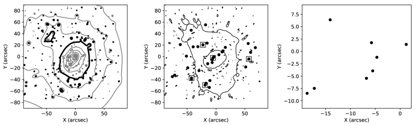
Figure 1: For the time delay test an existing model for Abell 1689 was used (Limousin et al., 2007), the mass distribution of which is depicted by contours in the left panel. There, the solid lines indicate $\kappa=1$ (for a source redshift of $z=3$); the spacing between contours is $\Delta\kappa=0.2$. The filled circles in the centre panel show the 32 image positions generated by the eight point sources in the right panel, the squares indicate the multiple image system that is used in the left panel of Fig 4. The critical lines shown in the centre panel also refer to a redshift of $z=3$.

3.2 Generalizations

The dynamic grid that is used in the inversion strategy serves to fix the positions and sizes of the Plummer basis functions, for which the GA will subsequently determine the weights. For the GA itself, it is however irrelevant that the positions and sizes originate from a grid layout, and this has been made explicit: while the user of the inversion code can still work with the existing and tried subdivision procedure, there is now the option of using a different way to determine this layout of basis functions. In sections 5 and 6 this is used to facilitate handling both small scale substructure and large scale weak lensing measurements.

In a similar way, the choice of basis function is not relevant to the GA, in the sense that once the necessary deflection angles have been calculated, it does not matter from which type of basis function they originate. The specific choice will certainly have an effect on how well the GA will converge to a solution and how well this solution will perform, but it does not change the inner workings of the GA. Therefore, the inversion code can not only be instructed where to place the basis functions in a more flexible way, but the type of basis function can be specified as well. Any type that is supported by the Grale simulation code can be used here, ranging from simple models like a projected Plummer sphere, a square pixel (Abdelsalam et al., 1998) or a singular isothermal sphere (SIS) over rotated elliptical models to even complex composite models. Moreover, different basis functions need not originate from the same underlying models, different ones can be used, e.g. Plummer basis functions augmented by a few SIS models. The use of the mass sheet basis function can be generalized as well: if desired, any other supported model can be used instead. While this can be a model with a similar effect, e.g. a mass disc instead of a mass sheet, this does not need to be the case. Note that the GA still treats this type of basis function slightly differently, as its weight is not included in the rescaling step mentioned earlier.

3.3 Fitness criteria

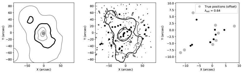
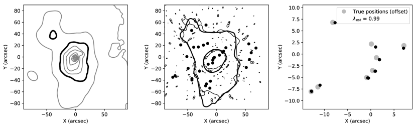
Figure 2: Results for the time delay test, where the multiple images from Fig. 1 are used as constraints, augmented by time delay information for all image locations, as well as null space information. The top half corresponds to the use of $\textrm{fitness}_{\rm TD,2009}$, the bottom half to $\textrm{fitness}_{\rm TD,NoSrc}$. The recovered critical lines are shown as thick solid lines, the ones of the input lens as thin lines for comparison. In the right panels, which show the back-projected images (i.e. the estimate of the sources), the true source positions are indicated as well, as filled gray circles with a diameter of 1”, but offset to have the same centre as the recovered positions. This allows one to compare the relative sizes of input and reconstructed source planes, thereby visualizing a rescaling due to the MSD. The estimated scale factor $\lambda_{\rm est}$ corresponds to this fraction of recovered to true source plane areas, and would quantify the relation between the reconstructed and real mass densities according to equation (14) in case the exact MSD would apply. The older time delay fitness measure causes over-focusing of the images, while the new fitness criterion allows the MSD scale factor be recovered accurately. This MSD difference is also hinted at by the difference in number of density contours, indicating that one solution is steeper than the other.

Central to the optimization procedure are the fitness criteria: each one provides a measure of how well a trial solution performs for some specific aspect. In the GA that is used in Grale, the precise value of these fitness measures does not matter, they are only used when comparing two genomes to determine which one is better. If more than one fitness measure is used, roughly speaking, a genome is said to dominate another one if it is better with respect to all these fitness values. In a set of genomes one can then identify the subset that is not dominated by any other genome: the non-dominated set. After excluding this subset, a new non-dominated set can be determined and so on. If only a single fitness measure is specified, the trial solutions can be ranked accordingly; if more than one fitness type is used, the population of genomes is subdivided into these non-dominated sets. At the core however, one only needs to be able to tell which solution is better regarding a single fitness criterion, there is no need for differentiability or even continuity of these fitness measures.

In a strong lensing scenario, the central requirement is that different images originate from the same source. If extended images are used as input to the inversion routine, this requirement is translated into a fitness measure that projects the images onto their source planes, and for these back-projected images measures how well they overlap. This is done by measuring the distances between the corners of rectangles surrounding the back-projected images, and the distances between corresponding image points when available. Such distances are not measured on an absolute scale however, instead, the average size of the back-projected images is used. As described in Liesenborgs et al. (2006), this helps guard against solutions that over-focus the images. Note that in this approach differently sized images are matched to a single source size, thereby incorporating information about the magnification of the images as a whole as well (the magnification of unresolved points is not used). For the more complex situation of merging images on a critical line, some care should be taken so that these partial source shapes are not compared directly to the full source shape from another, complete image. One could either use only part of the full image, the part that is visible in the merging ones, or, if the images are particularly extended and corresponding points can be identified in all images, only use these to determine the overlap and not the rectangles.

The identification of extended images is not always straightforward however, and it is actually more common to have point image information instead. If this type of input is used, the back-projected image sizes are no longer available to base a distance scale on. Instead, as described in Zitrin et al. (2010), the size of the area of all back-projected image points is used. This places some control over the GA in the hands of the outermost sources, as they determine this scale, which in turn affects the calculated fitness value. If one wants to guard against this, it is possible to base this scale on the median absolute deviation (MAD) of the back-projected positions, at the expense of some additional computations. In this point image approach, using magnification information of the point images is not available as a constraint in the optimization procedure.

These ‘overlap’ fitness measures work in the source plane, and while the choice of the distance scale used for measuring overlap avoids preferring trial solutions that merely over-focus the images, in essence it remains a source plane optimization. The back-projected images will not coincide perfectly, and because only a source plane criterion is used, there is no guarantee that these differences will stay small in the image plane (see also Kochanek (2006)). The root-mean-square (RMS) value of the predicted vs provided image positions can be used to measure this, and in practice this has turned out to be very acceptable using the fitness measure above. In case a relatively bad RMS is obtained, or if one would like to improve it even more, a fitness measure based on the differences in the image plane instead of the source plane can be used. To do so, these differences in the image plane $\Delta\mbox{\boldmath$\theta$}$ are approximated by multiplying the corresponding difference in the source plane $\Delta\mbox{\boldmath$\beta$}$ with the inverse of the magnification matrix $\mathcal{A}$ (see equation (6)), similar to the approach in Oguri (2010), appendix 2. Specifically, for a set of corresponding image points, each of the back-projected points in turn is used as a possible source position, and differences with other back-projected positions are translated into image plane differences using the magnification matrix. The sum of these squared differences is the basis for the fitness measure. To avoid sources with more images having a disproportionally large influence during the optimization, per source the average of this sum is used. The complete fitness value, for all sources, then consists of the sum of these single source contributions. By itself this fitness criterion does not seem to yield source plane points that overlap as well as the other overlap fitness measures, but using both fitness measures together in the multi-objective GA usually provides solutions which perform well on both accounts – at the expense of an extra fitness criterion however.

Depending on the number of observed images that can be used for the lens inversion, it may be possible for the GA to evolve towards a solution that, while correctly predicting the input images, also predicts unobserved extra images. To help the GA steer clear of such sub-optimal solutions, an additional null space fitness measure can be specified. For a source with extended images, one typically creates a grid of triangles encompassing a part of the image plane, where not only regions containing the observed images are cut out, but also regions where unobserved images are possible, e.g. behind bright cluster galaxies. By projecting these triangles onto the source plane and determining the amount of overlap with the estimated source, a value is obtained that expresses if there are extra images and how prominent they are (Liesenborgs et al., 2007). For point images, a more straightforward approach is used: there, a simple uniform grid of triangles is used, i.e. no regions are cut out, and the number of back-projected triangles that overlap with the estimated source are counted, thereby providing a rough estimate of the number of images of the source (Zitrin et al., 2010). For both approaches, the grids have typically been based on a uniform subdivision of an image plane area ranging from $48\times 48$ to $64\times 64$ square grid cells, each cell consisting of two triangles. Specific regions, e.g. the observed images, can be removed from this uniform grid automatically. The grid is taken to be larger than the area of the images themselves to avoid failing to detect extra images that lie farther away from the central region – which would not overlap with any of the triangles.

In Liesenborgs et al. (2009), a fitness measure was described in case time delay information is available, to study the constraints provided in the SDSS J1004+4112 lensing system. In section 4 we shall introduce an alternative formulation and investigate the performance of the existing and new fitness measures.

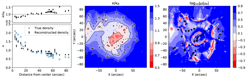
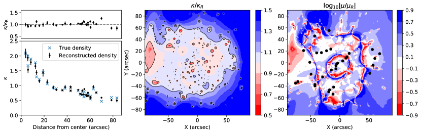
Figure 3: In each of the three panels, the top figure corresponds to the solution obtained with $\textrm{fitness}_{\rm TD,2009}$ and the bottom figure to the one obtained with $\textrm{fitness}_{\rm TD,NoSrc}$. Left panel: the larger plots show both input and recovered densities measured at the positions of the images, while the smaller ones show the fraction of the recovered density $\kappa$ to the real density $\kappa_{R}$. For visualisation purposes, only the distance of a point to the coordinate centre is shown on the horizontal axis. Whereas the newly proposed fitness measure yields densities that match the true ones well, the other one produces solutions which are less steep, and which have a more prominent density offset, i.e. that differ by the MSD. Centre panel: these maps show the $\kappa/\kappa_{R}$ fraction in the region under consideration. The solid black line marks the 10% boundaries. While the $\textrm{fitness}_{\rm TD,2009}$ solution has clear difference in both the central and outer regions, similar as what can be seen in the left panel, the solution obtained with the new fitness measure is well constrained over a large area. Right panel: these plots compare the magnification of the recovered lens model $\mu$ to the true magnification $\mu_{R}$, both for a redshift of $z=9$. The consistently larger magnification for the older fitness measure is again a sign of the MSD. The new $\textrm{fitness}_{\rm TD,NoSrc}$ on the other hand produces a much more consistent map.

While Grale is designed for the inversion of strong lensing systems, having information about the larger, weak lensing region is becoming increasingly common. It would therefore be desirable to be able to integrate the available weak lensing measurements into the inversion procedure. Section 6 formulates a fitness measure that can be added to the multi-objective GA, and investigates the information that can be retrieved in this way, for various degrees of correctness of the weak lensing shear estimates.

4 Time delays

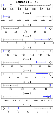
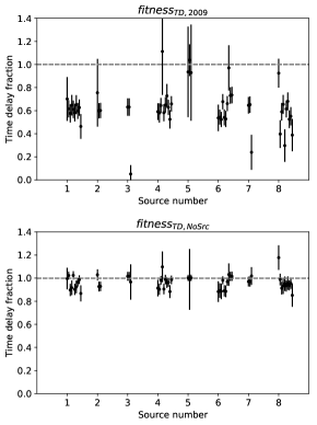
Figure 4: Left panel: this figure compares the predicted time delays to the input ones (diamond symbol) for all image pairs of one particular source, indicated by squares in the centre panel of Fig. 1; the time delays are shown as a number of days. The dotted black line shows the average and standard deviation when the existing $\textrm{fitness}_{\rm TD,2009}$ is used, whereas the solid blue lines correspond to the new $\textrm{fitness}_{\rm TD,NoSrc}$. For this system, as well as the ones that are not shown in the figure, the latter fitness measure produces time delay predictions that correspond better to the input time delays. Right panels: instead of showing the time delays themselves for all image pairs, these figures show the fraction of predicted time delay to true time delay for all sources, and for all image pairs per source. The error bars again indicate averages and standard deviations. Clearly, the new fitness measure provides much better correspondence with the true time delays. The fact that $\textrm{fitness}_{\rm TD,2009}$ produces time delays that are consistently shorter can be largely attributed to the MSD, which would scale time delays by a certain factor.

When available, time delay measurements between images of the same source provide especially valuable information. As shown in equation (5), they directly probe (non-local) differences of the projected potential. The image positions themselves only provide information about its gradient (equation (2)), and local image deformations even only sample the curvature of the projected potential. As explicitly demonstrated in Liesenborgs & De Rijcke (2012), time delay information is therefore very useful in breaking the MSD.

The original fitness measure for including time delay information is based directly on (5). That equation mentions a single source position however, which is not known at optimization time, and for this reason each of the back-projected image points $\mbox{\boldmath$\beta$}_{k}=\mbox{\boldmath$\beta$}(\mbox{\boldmath$\theta$}_{k})$ is used as a possible source position. Calling

$$\Delta t_{ij,kl}\equiv t(\mbox{\boldmath$\theta$}_{i},\mbox{\boldmath$\beta$}_{k})-t(\mbox{\boldmath$\theta$}_{j},\mbox{\boldmath$\beta$}_{l})\mathrm{,}$$ (15)

the time delay fitness contribution for a single source was given by

$$\textrm{fitness}_{\rm TD,2009}=\sum_{i\in T}\sum_{\begin{subarray}{c}j\in T\\ j\neq i\end{subarray}}\sum_{k=1}^{N}\sum_{l=1}^{N}\left(\frac{\Delta t_{ij,kl}-\Delta t_{{\rm obs},ij}}{S_{ij}}\right)^{2}\mathrm{,}$$ (16)

where the subscript 2009 refers to Liesenborgs et al. (2009), where this equation was introduced. The set $T$ is the subset of image positions for which a time delay measurement exists, $N$ is the number of images of the source under consideration, and in case multiple sources with time delays are available these contributions are simply added. The comparison scale $S_{ij}$ is by default set to $\Delta t_{{\rm obs},ij}$, administering all time delays the same relative importance. As this may be impractical in case a time delay is close to zero for example, a different scale value may be set instead.

Remembering that this fitness measure will be used in conjunction with the default positional fitness, the effort to compensate for the unknown source position in the expression above actually appears to incorporate this overlap requirement as well. Interestingly it has been shown in e.g. Borgeest & Refsdal (1984) and Gorenstein et al. (1988b) that the source position can be eliminated from the time delay expression: expanding the expression for $\Delta t_{ij}$ and noting that $\mbox{\boldmath$\beta$}=\mbox{\boldmath$\theta$}_{i}-\mbox{\boldmath$\alpha$}_{i}=\mbox{\boldmath$\theta$}_{j}-\mbox{\boldmath$\alpha$}_{j}$, one finds

$$\Delta t_{ij}\propto\frac{1}{2}(\mbox{\boldmath$\theta$}_{i}-\mbox{\boldmath$\theta$}_{j})\cdot(\mbox{\boldmath$\alpha$}_{i}+\mbox{\boldmath$\alpha$}_{j})-\psi(\mbox{\boldmath$\theta$}_{i})+\psi(\mbox{\boldmath$\theta$}_{j})\mathrm{,}$$ (17)

where $\mbox{\boldmath$\alpha$}_{i}\equiv\mbox{\boldmath$\alpha$}(\mbox{\boldmath$\theta$}_{i})$ and the proportionality factor is the same as in (5). Comparable to the fitness measure above, we can now base the time delay fitness on

$$\textrm{fitness}_{\rm TD,NoSrc}=\sum_{i\in T}\sum_{\begin{subarray}{c}j\in T\\ j\neq i\end{subarray}}\left(\frac{\Delta t_{ij}-\Delta t_{{\rm obs},ij}}{S_{ij}}\right)^{2}\mathrm{.}$$ (18)

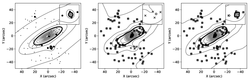
Figure 5: Left panel: the mass distribution used to study the situation where small scale substructure causes an extra quad to appear. Both large scale distribution and small perturbation are modelled using NSIE lenses, placed at $z=0.4$. The contours indicate lines of equal convergence $\kappa$, calculated for a redshift of $z=1.5$, which is the redshift of the multiple image system containing the quad (filled circles); the inset shows this region in more detail. The thick solid line indicates $\kappa=1$, the spacing between contours corresponds to $\Delta\kappa=0.25$. Small points indicate the other point images. Centre panel: the default subdivision procedure leads to this reconstruction, an average of 20 individual reconstructions. The input point images are shown as crosses, the corresponding images predicted by the model as open circles. As shown in the inset, the quad images cannot be reproduced, as the required density perturbation is not recovered. Right panel: similar to the centre panel, but this time extra basis functions were used to allow for a smaller resolution in between the quad images (see text). This time, the quad can indeed be reproduced.

Below we shall explore the relative performance of these two fitness measures, where the inversions were performed using the default grid-based approach to lay out the Plummer basis functions, and with a mass sheet basis function enabled. Apart from the positional and time delay fitness measures, the null space criterion was used as well. The lens model used is the Lenstool one for Abell 1689 (Limousin et al., 2007), which is merely used as a an example of an underlying true mass density, i.e. the simulated images have no relation with the images observed in that cluster. Instead, eight source positions were chosen, generating 32 images. To assess the effect of adding the time delay fitness measures, in these tests all of the multiple image systems were equipped with time delay information.

Neither in this test, nor in the ones in the next sections, the true lens model originates from an N-body simulation. The non-parametric inversion method uses a multitude of basis functions to be able to model mass distributions with rather arbitrary shapes, implying that the origin of the observed images should not matter. The images can be based on simulations using an analytical model, as in this example, using more complex N-body simulations, e.g. as in Meneghetti et al. (2017), or, of course, real world observations. To assess properties of the reconstruction procedure in general, one would not want to be restricted by the kinds of models that N-body simulations produce, but allow more flexible mass distributions, e.g. differing by an MSD-like scale factor, as well.

The true lens as well as the generated images and corresponding sources can be seen in Fig. 1. The reconstructions for this system, for both fitness measures, are depicted in Fig. 2. In the top half, where $\textrm{fitness}_{\rm TD,2009}$ was used, the contours of the recovered density indicate a distribution that is less steep, and has a larger density offset than in the bottom half, for $\textrm{fitness}_{\rm TD,NoSrc}$. A similar effect can be seen when comparing both reconstructions in the left panel of Fig. 3, where the densities at the locations of the images are shown, and is highly suggestive of the presence of the MSD. The centre panel of the same figure shows the fraction of the recovered density $\kappa$ to the real density $\kappa_{R}$, in the part of the lens plane under consideration. Whereas the recovered density using $\textrm{fitness}_{\rm TD,2009}$ only lies within 10% of $\kappa_{R}$ in a relatively small region, the correspondence for the newly proposed fitness measure clearly covers a much larger region, with main differences where the mass peaks in the true model are located.

This MSD effect can also be seen in the right panel, where the magnification is shown for a source at a redshift of $z=9$, similar to figs 21 and 22 of Meneghetti et al. (2017). Note that this redshift dependence causes the actual magnification of the images, which correspond to other redshifts, to differ. As the magnification can change over orders of magnitude, we have chosen to plot the logarithm. The consistently different magnification for the old fitness measure is again a manifestation of the MSD, which is far less problematic with the new fitness measure. Still, being dependent on second derivatives of the projected potential, the magnification can be rather sensitive to small differences in models. For the new fitness measure, differences can therefore also be seen, although far less consistently, and most pronounced where there are no image constraints.

In the right panels of Fig. 2, the recovered sources are compared to the input source positions, where the latter are offset to have the same centre location. In a gravitational lensing scenario, the overall offset of the source positions cannot be constrained, as is explained in more detail in appendix A. By using this offset in the plots, the scales of the recovered vs. input source planes can however easily be compared visually. The exact MSD from equation (14) as well as the generalized versions cause differently scaled source planes to correspond to the same observed images, and the estimated $\lambda_{\rm est}$ from these recovered and real source plane scales can therefore be used to indicate the degree to which the correct solution has been retrieved. Note that the relation between source sizes and image sizes is precisely what the magnification corresponds to, so the consistently larger magnification in the top-right part of Fig. 3 is to be expected based on this difference in source plane scales.

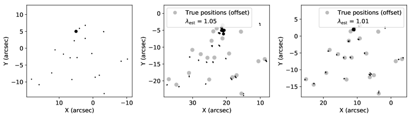
Figure 6: Left panel: the 20 true source positions, that generate the multiple image systems shown in the left panel of Fig. 5. Here too, the source responsible for the quad is shown as a filled circle. Centre panel: the back-projected images using the reconstruction in the centre panel of the same figure, compared to the true source positions; the diameter of the gray circles is 1”. Similar to a previous example, the true source positions are shown with an offset, to be able to compare true and recovered source plane scales. While the overall scale is recovered well, as are most sources, especially the images of the quad system do not coincide satisfactorily. Right panel: same, but using the reconstruction of the right panel of Fig. 5. The agreement of the source plane scales is even more similar, but especially noticeable is the fact that the points of the quad system now overlap to a much better degree.

Based on these results, using the newly proposed fitness measure appears to be advantageous, as both densities at the images positions and scale of the source planes are recovered more accurately. To further assess the performance of the two time delay fitness measures, the time delays that were provided as input will be compared to the predicted time delays, which are calculated as follows. First, the image points for the same source are projected back onto their source plane and their average – the straightforward average, not using weights based on the magnification – is used as the source position $\beta$. The image positions $\theta$ that correspond to this $\beta$ are recalculated, yielding image position predictions that differ somewhat from the input positions. This $\beta$ and these $\theta$ positions are subsequently used to calculate time delay differences using equation (5), and finally compared to the input time delays. In this experiment 40 individual solutions were generated to estimate accuracy and precision.

The left panel of Fig. 4 shows the averages and standard deviations, based on the 40 individual solutions, of the time delay predictions for this test, for the images of a single source. The dotted black line shows these quantities for the existing fitness measure, whereas the solid blue line shows those for the newly proposed one. Plots for the other sources show the same trends, which can in fact be more clearly seen in the other parts of the figure, where for each source, and each image pair, the time delay fraction $\Delta t_{ij}/\Delta t_{ij,{\rm obs}}$ is shown. The quite consistently smaller time delay sizes for $\textrm{fitness}_{\rm TD,2009}$ can again be seen as an MSD effect, rescaling the projected potential as well as the density. For this test, the effect is quite clear: the new fitness measure which eliminates the unknown source position produces predictions that match the input time delays to a much better degree.

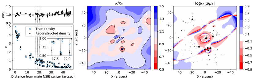
Figure 7: Left panel: using the recovered mass map shown in the right panel of Fig. 5, the densities $\kappa$ at the positions of the images are compared to the densities of the real lens, $\kappa_{R}$; the positions of the quad images are indicated by vertical lines, more clearly discernible in the inset. While there are certainly differences, the overall steepness as well as the density offset appear to be recovered correctly. Centre panel: the relative density, $\kappa/\kappa_{R}$, of recovered and true lens models, over the lens plane region; the black line again indicates a change of 10%. This boundary covers a large part of the region, with a notable exception at the position of the quad, indicating that further, more local degeneracies can play a role. Right panel: comparison of the recovered magnification $\mu$ to the one of the real lens model, $\mu_{R}$. The correspondence shows much less variation as compared to the example in Fig. 3, undoubtedly due to a less complex mass model needing to be recovered.

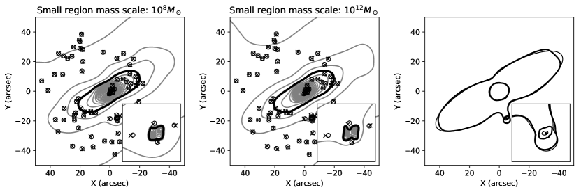
Figure 8: The first two panels show results similar to the right panel of Fig. 5, but for different settings of the mass scale in the region of the small density peak (see text). The right panel shows the critical lines at the redshift $z=1.5$ of the source, for both the reconstruction from the right panel of Fig. 5, and the true lens.

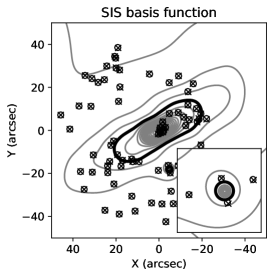
Figure 9: Instead of using a grid of Plummer basis functions to account for the small scale substructure, one can imagine that based on the visible light a single basis function is used. In this example, a SIS lens was placed at the centre of the mass peak inside the quad, and its weight was subsequently optimized during the inversion procedure. As shown, the resulting model is also capable of explaining the observed images, including the quad. For this inversion to succeed consistently, the extra RMS fitness measure needed to be enabled.

Source	1	2	3	4	5	6	7	8	9	10
Default RMS	0.17	0.22	0.16	0.25	0.27	0.12	0.11	0.14	0.17	0.067
Substructure RMS	0.24	0.19	0.15	0.26	0.20	0.15	0.092	0.14	0.15	0.078
Source	11	12	13	14	15	16	17	18	19	20
Default RMS	0.32	0.41	0.23	0.14	0.19	0.11	0.25	0.10	0.076	2.8
Substructure RMS	0.32	0.42	0.18	0.17	0.14	0.081	0.15	0.17	0.061	0.22

Table 1: For each of the sources used in the substructure test, the RMS comparing the true image locations to the predicted ones is specified in arc seconds. The first line, “Default RMS” shows the RMS that results from the default procedure, corresponding to the reconstruction in the centre panel of Fig. 5. The second line, “Substructure RMS”, are the values for the model in the right panel of the same figure. Only source 20, the one containing the small scale quad, shows a clear difference.

5 Substructure

The default procedure which uses the subdivision grid to arrange basis functions can have problems recovering small scale substructure: for basis functions with the required resolution to be present, one would need the mass threshold responsible for splitting a grid cell into four new cells to be relatively low, as such small scale substructure would not enclose a particularly massive region. This in turn causes other regions to be subdivided quite finely as well, leading to a very large number of basis functions. Without an adequate number of available constraints, the GA would easily evolve to a sub-optimal solution, essentially getting lost in the parameter space.

As mentioned in Williams & Liesenborgs (2019), this insufficient resolution was the case in the inversion of MACS J1149.6+2223. In that cluster, a well resolved background galaxy can be seen as three separate large images, and a supernova, SN Refsdal (Kelly et al., 2015), in one of the spiral arms was actually visible four times in one of these three images. This quad, with a relatively small separation, is generated by a cluster galaxy that overlaps with one of the larger images. The increased flexibility for placing basis functions that was described earlier, allows one to handle such cases with small scale substructure, where one has a strong indication that extra mass needs to be present at a particular location, for example because of the presence of a cluster galaxy as in MACS J1149, combined with a lack of accuracy in the initial reconstruction. While it has now become easy to add small scale substructure throughout the lensing region, in our opinion one should only make use of this when the default inversion procedure fails to recover something fundamental, e.g. the multiplicity of a lensed source.

To study a similar situation, the simulated gravitational lens shown in the left panel of Fig. 5 was used: the overall elliptical mass distribution at $z=0.4$ causes 81 images of 20 point sources, where four of the images are created by the presence of a carefully placed small mass clump at $(-4.8",-18.1")$, also shown in the inset. For both the main component and the small perturbation a non-singular isothermal ellipse (NSIE) model was used. The true source positions can be seen in the left panel of Fig. 6.

The centre panel of Fig. 5 shows the recovered mass distribution, an average of 20 individual solutions, when the default procedure using the dynamic subdivision grid is used. While the solution does hint at the presence of extra mass in between the quad images, a comparison of the input image positions (crosses) to the predicted image positions (circles) shows that the reconstruction does not have the required resolution to predict all images of the quad – in fact, only a single image position is recovered. The back-projected image positions, i.e. the estimated source positions, are shown in the centre panel of Fig. 6. While the overall scale of the situation is very similar to the one for the input sources, as can be seen from the $\lambda_{\rm est}$ value which expresses the fraction of these scales, and which indicates that the MSD scale factor and offset are recovered well, the back-projected images of the system containing the quad clearly overlap less well than the other ones.

To allow this source and the quad images to be recovered more accurately, in a small region in between these images other basis functions were added. Overall, the same subdivision steps were used as in the default inversions, but at each subdivision step basis functions based on a small, uniform $15\times 15$ grid were added as well. Given the paucity of constraints for the quad region, these extra basis functions should provide more than adequate flexibility. The result of this slightly modified procedure can be seen in the right panel of Fig. 5. Thanks to the extra basis functions available in between the quad images, mass could be placed there allowing the reconstructed lens to predict the existence of these images as well.

In the right panel of Fig. 6 the back-projected images are shown for this reconstruction, showing that the images of the system with the quad now overlap to a much better degree. The overall scale of the recovered sources still corresponds very well to that of the true sources, indicating that the MSD scale factor is found accurately. This is further supported by the left panel of Fig. 7 that compares the mass densities of the input lens to this reconstruction. While there certainly are differences, mostly near the main mass peak, the overall steepness appears very similar, as does the density offset. In fact, the similarity is within 10% of the true mass density for a considerable part of the lens plane area, as can be seen in the centre panel of the figure. The right panel compares the magnifications of the recovered and true densities, indicating a correspondence that could be expected from the matching source plane scales.

When comparing all back-projected images to the true sources, it does appear that the reconstruction in the right panel of Fig. 6 performs in general better than the one without the small scale basis functions in the centre panel. The true source positions are never an observable however, and as described in appendix A cannot be fixed. The only true criteria one can use to ascertain how well a reconstructed model fits the observations are how well the back-projected images correspond to a single source, and more importantly how well the re-traced images from the estimated source positions correspond to the observed images. For all multiple image systems except for the quad, both solutions, with and without the small scale substructure, perform similarly. This can be seen explicitly in Table 1, where the RMS for each system has been calculated in the following way: the average of the back-projected images is used as the source position, and starting from the observed image positions, these are modified to correspond to that source position. The table shows a clear difference for source 20, the one containing the quad, while the images of the other sources all have a very similar RMS in the two reconstructions.

For each set of basis functions, the GA will look for appropriate weights. The initial weights, e.g. the initial masses of the Plummer basis functions, as well as their relative contributions will of course affect this search. For the overall mass distribution, the total mass required is automatically estimated from the separations in the multiple image systems, and the initial weights are chosen to correspond to this total mass. For the extra basis functions, which are needed to reproduce the quad images, no such automated procedure is provided however, and an extra mass scale for this region needs to be provided manually. In the reconstruction shown in the left panel of Fig. 5, this mass scale was set to $10^{10}M_{\odot}$.

Fortunately, the procedure does not appear to be very sensitive to the choice of this initial mass scale, as can be seen in Fig. 8. There, similar reconstructions are shown, only differing in this mass scale for the small region, changing over four orders of magnitude, from $10^{8}M_{\odot}$ to $10^{12}M_{\odot}$. The details are different, as there are only very few constraints for the small region, but in each case a reconstruction could be found. The addition of a small null space constraint, only for the region around the quad, was helpful in preventing the optimization from placing too much mass there, mainly for the larger mass scales. The right-most panel compares the recovered critical lines to the ones of the true lens. While there are some differences, which can be expected due to the lack of constraints in the region of the small mass density peak, the overall correspondence is good.

Instead of using a grid of Plummer basis functions to be able to account for a wide variety of mass distributions in between the quad images, one could imagine using a single, more simple density profile. To illustrate that the extensions to Grale now make it possible to combine the default, Plummer basis functions with a different one, here we use a single SIS basis function inside the quad. While the previous approach certainly aligns better with the non-parametric philosophy of this inversion procedure, there may be cases where a lack of constraints suggests such an approach. The result of this, again an average of 20 individual reconstructions, is shown in Fig. 9. In this case, the null space in the quad region was no longer enabled, but unfortunately only using the overlap fitness did not consistently predict the quad with acceptable accuracy. Enabling the RMS fitness measure in conjunction with the standard overlap fitness improved the results considerably, and, as the image shows, the resulting model can successfully reproduce the quad.

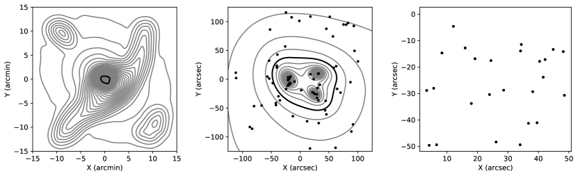
Figure 10: The simulated gravitational lens, at $z=0.4$, used in the weak lensing tests. Left panel: the large scale mass structure that will be probed by ellipticity measurements with varying degrees of accuracy. The thick line corresponds to $\kappa=1$ for a redshift $z=3$. To make the large scale structure more clearly visible, the contours are separated by a small $\Delta\kappa=0.025$. Centre panel: the strong lensing region of the same mass distribution. The thick line again corresponds to $\kappa=1$, while the contour spacing is now $\Delta\kappa=0.2$. The dots indicate the positions of the 75 point images that are included as constraints. Right panel: the 25 point sources that cause the images from the centre panel.

Figure 11: Illustrations of the input ellipticity data used in the three scenarios for the weak lensing tests. First (left most) panel: in scenario (A), the input is the exact ellipticity information calculated from the true model, on a $48\times 48$ grid. Here, the orientation and sizes for $z=1$ are shown; the inset shows the size of $|\epsilon|=1$. Second panel: similar, but for scenario (B), where 25 random source ellipticities were transformed at the grid points, and averaged. The result is a more noisy version of the previous ellipticities. Third panel: for scenario (C), 12,000 source ellipticities at different redshifts were transformed. These were binned according to redshift, and on a $48\times 48$ grid the weighted averages were calculated. The last panel shows the result for the bin corresponding to $z=1.5$, one of the inputs in scenario (C). To avoid the less correct weak lensing data affecting the more accurate strong lensing constraints, the central $2^{\prime}$ region was excluded.

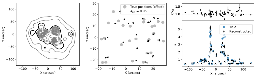
Figure 12: Using only the strong lensing constraints for the simulated lens of Fig. 10, these results are obtained. Left panel: the average mass map of 20 individual runs, where the mass sheet basis function was included. The general features of the true mass distribution could be recovered. Centre panel: comparing the true source positions to the back-projected images shows that overall, the scales correspond well, although there is slight over-focusing. The diameter of the filled gray circles is 2”. Right panel: a comparison of the true and recovered densities at the image positions, of which the $x$-coordinate is used on the horizontal axis, shows no obvious differences in density offset or steepness.

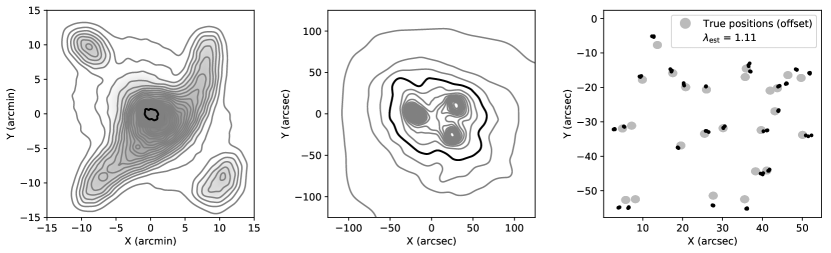
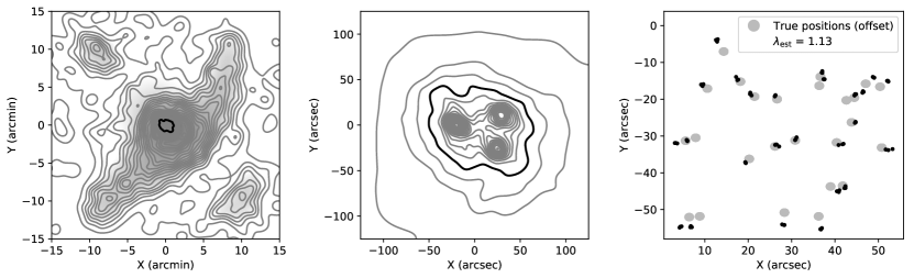
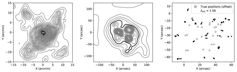
Figure 13: The three rows correspond to inputs (A), (B) and (C), obtained when the mass sheet basis function is not used. The left panels show the wide area reconstruction, mainly due to the weak lensing data, where the background shows the shape of the true mass density for comparison. To make the small features better visible, a logarithmic gray scale was used. The centre panels show the reconstructions of the strong lensing regions, all having quite similar features. While the overall shapes are similar, the contour spacing in scenario (C) shows a steeper mass map. The right panels show the back-projected images in each case. While consistent source positions as well as the source plane scales could be recovered for scenarios (A) and (B), the scales differing by 11 and 13% respectively, for scenario (C) neither do the back-projected images overlap well, nor is the scale of the back-projected images consistent with the true source plane scale. The size of the filled gray circles is again 2”.

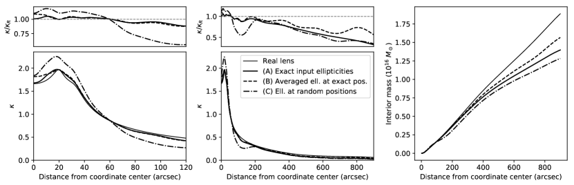
Figure 14: When no mass sheet basis function is used, these profiles are recovered in the weak lensing test. Left panel: the circularly averaged densities in the strong lensing region show a good correspondence for inputs (A) and (B), as can also be seen from looking at the relative density $\kappa/\kappa_{R}$, however, the steepness and density offset are quite different when the input from scenario (C) is used. Centre panel: the circularly averaged densities over the entire weak lensing area. Interestingly, even though the strong lensing region is recovered incorrectly for scenario (C), beyond $\sim 200"$ the profile matches the other ones quite well visually, yet upon inspection of the $\kappa/\kappa_{R}$ ratio is becomes clear that actually all reconstructions underestimate the real density. Right panel: the integrated mass profiles as well show that in each one of the reconstructions the total mass is underestimated.

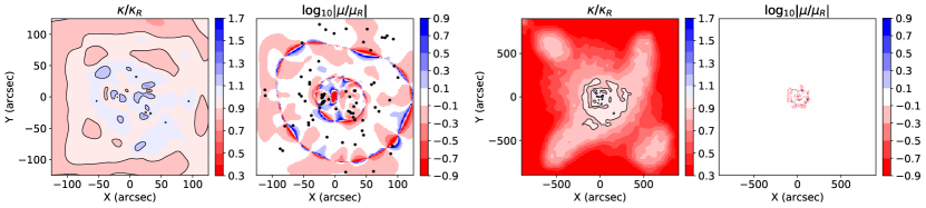
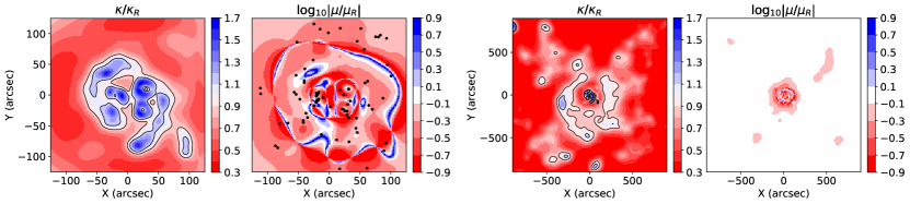
Figure 15: The three rows again correspond to scenarios (A), (B) and (C), and, for the inversions without enabling the mass sheet basis function, show the fractions of recovered densities and magnifications compared to the true ones. The left panels show these fractions for the strong lensing region, the right ones for the weak lensing region. Similar to the circularly averaged profiles, scenarios (A) and (B) show that in the strong lensing region the the density traces the true one within 10% (black solid lines) in the central part, while the weak lensing maps reveal a consistently lower reconstructed density. Not only is this underdensity present in (C) as well, but the different steepness in the strong lensing region manifests itself as only a very small part in the 10% range. The strong lensing magnifications confirm what could be seen in the plots of the source plane scales (right panels of Fig. 13: matching scales, and therefore magnifications, for (A) and (B), while the larger source plane scale for (C) corresponds to a lower magnification. For the wider weak lensing regions, the magnifications are more similar, in case (C) suggestive of different MSD scale factors for both strong and weak lensing regions.

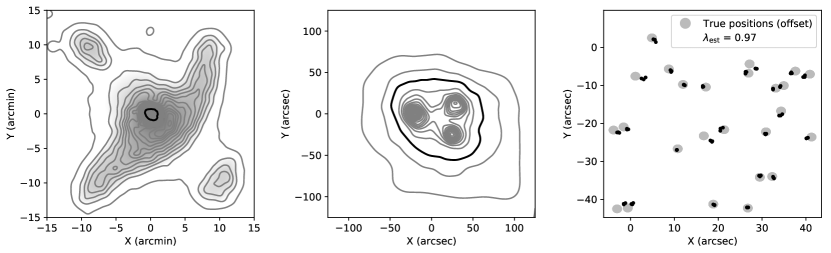
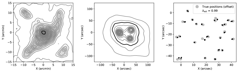
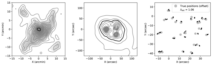
Figure 16: Similar to Fig. 13, but with the mass sheet basis function enabled. In all cases the structure shape in the weak lensing region is recovered (left panels), albeit with different levels of accuracy and somewhat different density offsets. The recovered strong lensing mass (centre panels) is very similar in each case, and the back-projected images overlap well (right panels). The recovered source plane scales match the true ones in all three cases, as can be seen from their $\lambda_{\rm est}$ estimates, indicating that the MSD scale factor is recovered well in the strong lensing region.

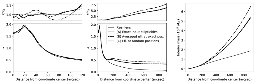
Figure 17: Similar to Fig. 14, but with the mass sheet basis function enabled. The circularly averaged profiles in the strong lensing region (left panel) show a very good correspondence to the true profile in all cases, as can also be seen from the plot of the relative density $\kappa/\kappa_{R}$. The profiles for the entire area (centre panel) not only show a considerable mass sheet for scenario (C), where the back-projected images show an improved reconstruction, but also for (A) and (B). The presence of a considerable mass sheet basis function in each case, does not only cause a large ratio of recovered versus true density in the outer regions, but also causes the integrated mass profiles to overestimate the correct enclosed masses in all scenarios (right panel).

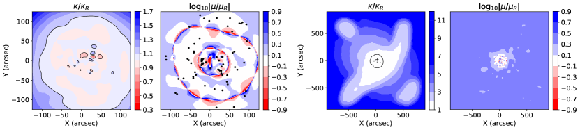
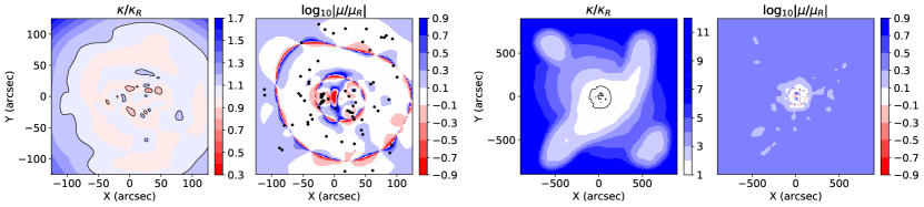
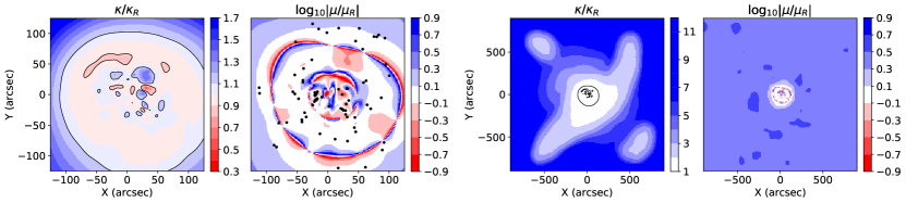
Figure 18: Similar to Fig. 15 but for the inversions where the mass sheet basis function was enabled. The strong lensing figures indicate a very good correspondence of reconstructed and real mass densities over most of the strong lensing region; the matching source plane scales can also be seen as matching magnifications. As can be expected from the circularly averaged density profiles, the situation is different when considering the weak lensing region. Not only is there a considerable relative overdensity in all three scenarios, the magnification is also larger than the true one in all three cases, different from the one in the strong lensing region.

6 Weak lensing

The positions of the multiply imaged sources that can be used to constrain the mass density in the strong lensing region, are often available with very good accuracy. The region in which multiple images are produced is limited however, but beyond this, the deformations of background galaxies may still provide additional information about the gravitational lens. As the intrinsic orientation of the background galaxies cannot be known, this weak lensing signal is statistical in nature.

To work with such information within the inversion framework of Grale, it is assumed that in a pre-processing step, the ellipticity information of the available background galaxies has led to estimates of the average ellipticity $\langle\epsilon\rangle^{\rm measured}_{i}$ at a number of positions $\mbox{\boldmath$\theta$}_{i}$. By calculating the reduced shear at these positions, equation (13) allows one to compare these measured values to the ones predicted by the model, $\langle\epsilon\rangle^{\rm model}_{i}$. This suggests the use of the fitness measure

$$\textrm{fitness}_{\rm WL}=\sum_{i=1}^{N}w_{i}\left|\langle\epsilon\rangle^{\rm measured}_{i}-\langle\epsilon\rangle^{\rm model}_{i}\right|^{2}\mathrm{,}$$ (19)

where there are assumed to be $N$ such measurements, and weights $w_{i}$ allow control over their relative importances if desired. Alternatively one could imagine using all ellipticity measurements directly, preventing overfitting the noise by an appropriate choice of a low number of basis functions. While the same fitness measure could still be used, this approach will not be explored in this article.

As the reduced shear is calculated by dividing the regular shear values $\gamma$ by the factor $(1-\kappa)$, these values can become large in regions where $\kappa$ is near its critical value, possibly even triggering a division by zero error during the optimization. To avoid such regions having a large effect during the course of the optimization, when the GA is still in the process of determining the very $\kappa$ map and a near-critical part of an otherwise good trial solution could cause it to be discarded, a threshold can be set for $|1-\kappa|$. Only points where $|1-\kappa|$ exceeds this threshold are included in the summation. In the reconstructions below, this threshold was set to $0.1$.

6.1 Simulated lens and reconstructions

To study the use of weak lensing data in Grale, the simulated gravitational lens shown in Fig. 10 was used. The shape in the strong lensing region (centre panel) is based on a lens model used in Liesenborgs et al. (2009), but embedded in the large scale structure shown in the left panel. Due to the use of this existing lens model, contrary to the other simulations this one used a matter density $\Omega_{m}=0.27$. The centre panel shows the 75 point images generated by the sources in the right panel. Three scenarios for the weak lensing input will be used, each time providing sets of $48\times 48$ values for $\langle\epsilon\rangle^{\rm measured}_{i}$, arranged on a uniform grid, covering the $30^{\prime}\times 30^{\prime}$ region.

In scenario (A), the ideal yet unrealistic case, these ellipticity values are in fact the exact values calculated from the model using equation (13). Furthermore, as weak lensing data at a single redshift do not provide enough constraints to fix the MSD scale, not even in the case of the exact MSD, let alone a generalization, three different redshifts, $z=1$, $2$ and $4$, were used to calculate the ellipticities for all grid points. The first panel of Fig. 11 shows the orientations (see equation (12)) and sizes of these data points, where the length of $|\epsilon|=1$ is shown in the inset. For scenario (B), a first degree of randomness was introduced: for each grid point, 25 random source ellipticities were transformed using equation (11), and these were subsequently averaged. As in the previous scenario, this was in fact done for the three redshifts of $z=1$, $2$, and $4$. This leads to a more noisy version of the true ellipticity field, as can be seen in the second panel of the figure.

In the third scenario, (C), a situation like one that could be encountered in practice is considered: similar to the weak lensing information that was made available for the mock clusters Ares and Hera (Meneghetti et al., 2017), 12,000 random source ellipticities at random redshifts were transformed by the real gravitational lens model, the result of which is shown in the third panel of the figure. These ellipticities were then distributed over a number of redshift bins, chosen to contain the same interval $0.1$ in $D_{ds}/D_{s}$ space. For each bin, for each of the grid points, the ellipticities were averaged using a gaussian weight function of size 1’; the right panel of the figure shows the result for one of the resulting redshift bins. The use of a gaussian weight function was also mentioned in Lombardi & Bertin (1998), to assign more importance to measurements close to the grid point under consideration. Other averaging methods exist as well, e.g. based on the points that lie inside a grid rectangle as in Cacciato et al. (2006), or even circular regions that are different in size, so as to contain a certain number of ellipticity measurements (Merten et al., 2009). To illustrate the issues that may arise from combining strong and weak lensing measurements, the chosen method suffices. To avoid the lower accuracy weak lensing signal inside the strong lensing region interfering with the more accurate strong lensing data, a central circular region with a $2^{\prime}$ radius was excluded in this case. As the central region tends to contain bright cluster galaxies, it is furthermore not unlikely that only little ellipticity information of background galaxies would be gathered there.

Note that in all scenarios the ellipticity measurements themselves are still assumed to be entirely correct. The only sources of error are the number of measurements available to obtain an estimate of the average value (scenario (B)), as well as the spatial distribution of the measured ellipticities (scenario (C)). In settings (A) and (B), no different weights were provided; in (C) the number of ellipticity measurements in the redshift bin was used as weight $w_{i}$.

To be able to assess the added information provided by the ellipticity data, not only in the wider weak lensing region but in the central, strong lensing region as well, for reference Fig. 12 shows the results when using only the information from the multiple images, as well as the null space. As is usual in these kinds of reconstructions with Grale, the aforementioned mass sheet basis function was included. For these results, and in the other inversions that follow as well, the average solution of 20 runs is shown. As the left panel shows, the general features of the central region are recovered, and as the relative densities $\kappa/\kappa_{R}$ are centered on 1, based on the densities at the image positions no clear MSD scale factor can be detected. As can be expected from this correspondence, the scale of the recovered source planes is only slightly different from the true one, as the central panel shows, the estimated scale factor $\lambda_{\rm est}$ differing by only a few percent.

For the next inversions that we shall consider, apart from the strong lensing fitness measure for point images, $\textrm{fitness}_{\rm WL}$ is enabled in the multi-objective GA as well. The null space fitness measure was not needed to avoid spurious structures in the recovered mass maps. To provide the Plummer basis functions of which the weights need to be optimized, an approach similar to the one used in the example from section 5 is used, but this time for the wide area instead of a very small one: as in other inversions, the different steps with the subdivision grid is used for the strong lensing region, and to be able to model the weak lensing region as well, in every step extra basis functions are added that cover the weak lensing region, laid out according to a uniform $48\times 48$ grid. Originally, a mass sheet basis function was introduced because the strong lensing region could contain a non-negligible density offset that may be difficult to model using several separate Plummer basis functions. Now that the inversion area is much wider, and assuming that the density near the border of the region will be low, it makes sense to expect the weak lensing signal to recover the overall structure, and thereby provide the required density offset inside the strong lensing region. The results shown in Figs 13 and 14 are therefore the ones obtained without enabling a mass sheet basis function.

The three rows in Fig. 13 correspond to the three different scenarios that were described earlier. The top row, in which the true average ellipticities were used as constraints – scenario (A) – recovers the wide area structure very well. The centre panel, showing the strong lensing area displays a good agreement as well, while the back-projected images in the right panel do indicate slightly larger source plane scales, although the effect is limited to 11%. While the input ellipticity data is overly optimistic, this scenario does illustrate that Grale is able to combine weak and strong lensing constraints and the code works as expected. The next row, where the results of scenario (B) are shown, is actually quite similar, but the reconstruction in the weak lensing region is clearly more noisy. The third row, showing the results for the more realistic scenario (C) is certainly the more interesting one. While the overall structure in the weak lensing area is still visible, the result does not provide the same accurate representation of the shape of the mass as before. This could be expected, as the input ellipticity map is diluted by the gaussian smoothing. Looking at the contours in the outer regions, it becomes clear that less mass is recovered there. The strong lensing mass does contain the expected features, but the back-projected images show that not only the reconstruction was not successful in producing well overlapping points, but that the scale set by these points differs by over 50% from the one set by the true sources.

This difference suggests the presence of the MSD, which can clearly be seen in the left panel of Fig. 14, where this last solution is steeper and has a lower mass offset than the true lens, as well as the other two reconstructions. Interestingly, the centre panel indicates that beyond $\sim 200"$ the profiles of the reconstructions do resemble the true profile, although the relative density $\kappa/\kappa_{R}$ of recovered to real models shows that it is consistently and increasingly underestimated. This can also be seen in the right panel, showing the total enclosed mass vs. radius, indicating that not all mass has been captured by the reconstructions. This is not only the case for the reconstruction using input (C), but even for (B), as well as for the very correct looking solution for (A).

Fig. 15 shows relative densities and magnifications of recovered and real lens models, in both strong and weak lensing regions. In scenarios (A) and (B) the main difference is the density in the wider, weak lensing area, but for (C), the strong lensing region as well shows considerable differences. The difference in source plane scale can be seen as a consistently lower magnification. While the difference in steepness and mass offset in the strong lensing region, as well as the different magnification can all be attributed to the MSD, the fact that the magnification deviates with a different factor in strong and weak lensing regions suggests a different MSD-like effect in both regimes.

Disabling the mass sheet basis function was prompted by the idea that the reconstruction in the weak lensing area would provide any mass sheet like effect that might otherwise be difficult to account for. But as the previous reconstruction for input (C) still seems to suffer from the MSD, and this was not the case for the strong lensing only reconstruction, it is interesting to see the effect of the inclusion of such a basis function. Similar to the previous figures, Figs 16, 17 and 18 show the results for these inversions, this time with a mass sheet basis function enabled. The left panels of Fig. 16 show that in all three cases the shape of the wide area mass distribution does seem to be recovered, albeit with different mass offsets, slopes and level of detail. The centre panels show strong lensing masses that are very similar to the true mass distribution there, and the right panels indicate that the recovered source plane scales correspond very well to the true ones.

That the MSD scale factor is obtained correctly, at least in the strong lensing region, can also be seen in the left panel of Fig. 17, where all profiles now have similar steepness and offset, and in the left part of Fig. 18. In the right part of that figure, showing the wider area, as well as in the centre panel of Fig. 17, the presence of the mass sheet basis function becomes very obvious however. The integrated mass, in the right panel, is therefore clearly larger than the correct one in all three cases. Whether or not there is non-negligible density in the outer regions, and using a mass sheet component may be warranted, will depend on the situation. As this example illustrates, it may however not be straightforward to determine this automatically. While the correctly estimated source plane scales in the strong lensing region can be seen as matching magnification ratios in the left part of Fig. 18, the situation is clearly different in the weak lensing region. The fact that there the magnification is consistently larger than the true one is again suggestive of different MSD-like scale factors in strong and weak lensing areas.

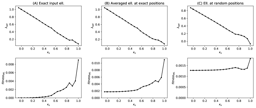
Figure 19: Based on the lens model with density $\kappa_{0}$ from Fig. 10, a new model is constructed: starting from a mass sheet with specific density $\kappa_{s}$, a factor $\lambda_{\rm opt}$ is determined numerically so that the new model $\kappa_{1}=\lambda_{\rm opt}\kappa_{0}+\kappa_{s}$ yields the lowest weak lensing fitness value. The columns indicate the different input scenarios for which this test was performed, the top row shows how, similar to the exact MSD (equation (14)), there’s a nearly linear relationship between $\kappa_{s}$ and $\lambda_{\rm opt}$, while the bottom row indicates that depending on the precise scenario, the relative fitness values do not change much.

6.2 Mass-sheet-like degeneracy

The fact that with this mass sheet basis function enabled, the shape of the mass density in the weak lensing area is still recovered well, is of course in itself a manifestation of the MSD. Whereas the last images show that in the strong lensing region the MSD scale factor is obtained correctly, in the weak lensing region a different one is obtained.

To better understand why the weak lensing data, containing information about different redshifts in each scenario, is not able to constrain this contribution better, a simple experiment is performed: starting from the true lens model $\kappa_{0}$ from Fig. 10, a new one is constructed in the following way. First, a mass sheet with a specific fixed density $\kappa_{s}$ is chosen. Next, a scaled version of the true lens is added where the scale is determined numerically to be the one that minimizes $\textrm{fitness}_{\rm WL}$, leading to the lens with the mass density

$$\kappa_{1}(\mbox{\boldmath$\theta$})=\lambda_{\rm opt}\kappa_{0}(\mbox{\boldmath$\theta$})+\kappa_{s}\mathrm{.}$$ (20)

The results are shown in Fig. 19, where columns refer to the different input scenarios (A), (B) and (C), the top row shows the scale factor $\lambda_{\rm opt}$ for each mass sheet density $\kappa_{s}$, and the bottom row shows the effect on the fitness measure. Note that these tests calculate $\textrm{fitness}_{\rm WL}$ for various lens models, constructed in the way described here, but do not use the GA based inversion procedure.

Similar to Seitz & Schneider (1997), where a distribution of redshifts is shown to still allow an MSD, the top row also shows a nearly linear relation for the best scale factor with respect to the density of the mass sheet. For scenarios (A) and (B), the lowest fitness value is for the true density map, or $\kappa_{s}=0$, indicating that in those cases the different redshifts successfully break the MSD. Note however that in scenario (C), while the lowest fitness value in the experiment is still for $\kappa_{s}=0$, the value for $\lambda_{\rm opt}$ actually differs from unity, i.e. a scaled mass map has a better fitness value than the true $\kappa_{0}$. Note that scenario (C) was obtained by using a gaussian weight function; in Lombardi & Bertin (1998) it is shown that the smoothed shear field then actually corresponds to a density map that is convolved with the same weight function, which can explain this observation. As the noise increases, the relative effect on the fitness becomes increasingly less prominent, and furthermore, the effect studied here is when the exact lens $\kappa_{0}$ is used, but in practice this is not the density that is available during the optimization. Instead, multiple basis functions are used to optimize the fitness measure, which may make the sensitivity to $\kappa_{s}$ even worse.

As also noted by Bradač et al. (2004), this experiment indicates that while in principle weak lensing data for multiple redshifts can break the MSD, in practice it is much less evident. It is therefore not surprising that when combining this information with the strong lensing data, and allowing for a mass sheet basis function, it is in fact the strong lensing data that dictates its value, causing a scaled mass density in the larger, weak lensing region.

For another way to look at this, let us assume that the strong lensing constraints and weak lensing constraints do not overlap. Based on the available data, one could perform a reconstruction for the strong lensing region, corresponding to a projected potential $\psi_{\rm SL}$. Similarly, one could perform a reconstruction based solely on the weak lensing measurements, leading to $\psi_{\rm WL}$. The former need not be valid in the weak lensing region, and the latter will only provide a very rough estimate in the strong lensing region. Let us next consider only the relevant parts of these potentials, $\psi_{\rm SL,central}$ for the strong lensing region, and $\psi_{\rm WL,nocentral}$ for the weak lensing region, both covering their respective constraints. As any value can be added to the potentials without affecting observables, one can imagine creating a $\psi_{\rm SL+WL}$ which is in essence $\psi_{\rm SL,central}$ in the central region, and $\psi_{\rm WL,nocentral}$ further out, using some interpolation in between. The combined potential will perform as well as both separate potentials in their respective regions, but the way the interpolation has occurred, obviously has an effect on the resulting mass density in between these regions, possibly allowing multiple equivalent lenses. Additionally, one can imagine that, if the MSD is not fully broken in neither strong nor weak lensing regions, both lensing potential parts can be first modified to create equivalent ones, and only then combined. The MSD scale factor would not even need to be the same for both parts, leading to even more equivalent lens models.

It is also interesting to note that the weak lensing constraints on the lensing potential are purely local ones, relating to only its curvature. One could therefore imagine different MSD contributions for different regions, for example a different mass sheet contribution as one moves further from the centre. As different regions may be differently sensitive to the MSD, this may be an additional effect to take into account, also easily affecting the total mass estimate.

6.3 Ring-like structure

The circularly averaged density plots from Figs 14 and  17 are not centred on one of the three mass peaks, but on the centre of the coordinate system. This highlights a feature which might otherwise be lost in the averaging procedure: in Fig. 14, the reconstruction for input (C) clearly shows a relative overdensity around $200"$. For scenarios (A) and (B), the effect is much less pronounced, but the reconstructed profile still deviates from the true one on the boundary between strong and weak lensing regions. In Fig. 17 a similar effect can in fact be seen in all scenarios.

Such effects have been encountered in other works where strong and weak lensing measurements were combined. In Diego et al. (2007) these ring-like structures were also perceived, followed by the argument in Ponente & Diego (2011) that such effects can be caused by overfitting. Interestingly, the work of Jee et al. (2007) identified a dark matter ring in Cl 0024+17 based on a combination of strong and weak lensing data. While the authors make a plausible argument for the possible origin of such a structure, further observations to confirm the existence are still awaited.

The discussion above about combining weak and strong lensing regions, each possibly having its own MSD, provides a possible explanation for such ring-like features, perhaps not surprisingly located on the border between the two regimes. More importantly, this has no intrinsic relation to the amount of overfitting, although depending on the precise method used, the degree of overfitting may affect the MSD in both regions, possibly separately, and can therefore be seemingly related to the introduction of such a feature.

7 Discussion and conclusion

In this article we have reiterated the current capabilities of the inversion procedure in Grale, a genetic algorithm based method, and investigated a number of upgrades that are now available. In this method, a number of criteria can be optimized concurrently, a common combination being the overlap of back-projected images, as well as the absence of unobserved, extra images, i.e. the null space. While the combined optimization of multiple aspects is certainly reminiscent of a regularization procedure, the criteria are not optimized together in the typical fashion of regularization, i.e. by combining multiple goodness-of-fit measures into a single number, with suitably chosen scale factors for the different aspects. Instead, a multi-objective genetic algorithm looks for a common optimum of the different so called fitness measures.

Which of the available fitness measures should be used will depend on the specific gravitational lensing system that is being studied. The basic requirement is having multiply imaged sources, but the addition of null space information may or may not cause improvements, depending on the amount of images, their spatial distribution and their redshifts. Because the inclusion of null space information causes the computational complexity to increase considerably, it is certainly worth exploring whether disabling the null space fitness already yields acceptable solutions, as more and more multiple image systems tend to become the norm: typically the null space will be most useful for the systems with fewest sources. Similarly, the fitness values describing a critical line penalty from Liesenborgs et al. (2008b) and Liesenborgs et al. (2009) were so far only needed in these works, where only very few sources were available.

Because of the flexibility of the basis functions used, in principle this now allows an approach that resembles the working of simply parameterized inversion methods: place basis functions such as a pseudo isothermal elliptical mass distribution (PIEMD, e.g Elíasdóttir et al. (2007)) based on the observed cluster members and optimize their contributions using the GA. Note however that, while this approach is certainly feasible, the GA can only change the weights of these basis functions, and not other parameters, such as ellipticity or orientation. How useful this feature turns out to be, for example to combine models of visible galaxies with a more non-parametric contribution, still needs to be investigated.

Time delays can provide very useful information about the overall lensing potential, and the time delay fitness measure proposed in Liesenborgs et al. (2009) was evaluated more thoroughly. The test was similar to the one used in Liesenborgs & De Rijcke (2012); Wagner et al. (2019), where a lens with an elliptical version of a Navarro-Frenk-White (NFW; Navarro et al. (1996)) mass distribution was used to gauge the effect of the addition of time delay information to the images of only a single source. Here, it was found that when adding time delay information to the images of all sources, the old fitness measure can over-focus the images whereas a newly proposed expression appears to avoid this. The same effect, although to different degrees, was seen in other tests as well, both with point images and extended images: the new time delay fitness measure yielded time delay predictions that were more compatible with the input time delays, and the resulting mass distributions suffered less from MSD effects. It is interesting to note that if the images of only one source were equipped with time delays, the over-focusing effect did not appear for the A1689-based test.

Especially in the application to MACS J1149.6+2223 (Williams & Liesenborgs, 2019) it was clear that the subdivision grid based procedure cannot always provide adequate resolution to account for all observed features. The updates to the inversion code include more flexibility regarding the basis functions used, thereby allowing small scale structures to be introduced when studying a gravitational lens simulation with similar features as MACS J1149, in turn causing the observed images to be predicted more accurately. In this approach, one can again use a number of basis functions to be able to describe a more general small scale mass distribution, or use a single profile, e.g. a SIS, guided by the observed light. As such small scale substructures may not have many constraints, it will depend on the specific case at hand which approach may be more appropriate. Note that in both cases, a manual intervention to account for small scale features is required, making the method less automatic, and perhaps somewhat less free-form. Investigating ways to automate this – e.g. adding substructure due to an underestimate of image multiplicity – will be the topic of further research.

While it appeared relatively straightforward to add weak lensing constraints as an extra fitness measure, the experiment shown revealed some interesting aspects. In Fig. 13, the first two scenarios show that if the quality of the ellipticity measurements supplied to the inversion is good, even allowing for some noise, the weak and strong lensing data can be combined quite successfully. However, even in the case where the ellipticity measurements are exact, the border between both regimes is visible in Fig. 14. An incompletely recovered total mass further indicates that the MSD scale factor was not fully retrieved: while the true model has a lowest convergence value of $\kappa=0.027$, the reconstructions have a minimum that is an order of magnitude smaller. As the weak lensing signal is further diluted in scenario (C), these measurements no longer provide a strong enough constraint in the strong lensing region to obtain an accurate MSD scale there. The result for the strong lensing region is then what is typically seen if the mass sheet basis function is not included: the algorithm does not succeed well in finding a model that creates overlapping back-projected images, as it is not straightforward to create an overall mass sheet like effect using several different Plummer basis functions. In scenarios (A) and (B) the weak lensing constraints on the other hand were effective in creating the right environment for the strong lensing data. In this sense, enabling the use of the mass sheet basis function can help in providing the right strong lensing environment, in all three scenarios. In that case, one can still learn about the general shape in the weak lensing region, but the precise mass density is clearly overestimated. If one is only interested in the strong lensing region, the inclusion of weak lensing data can be seen as having a sort of stabilizing effect, not unlike what was mentioned in Diego et al. (2007).

Breaking the MSD is not straightforward, not necessarily in the strong lensing region, not in the weak lensing region, and not in the combination of the two. Ultimately, the precise inversion method used, and in particular what kind of prior information it uses about the mass density that is expected, can make an important mark on the way the degeneracy is affected. This is what was visible in the examples shown, in various ways. In scenario (C) without the mass sheet basis function, the MSD scale factor was not obtained correctly in the strong lensing region, but was nevertheless combined with a more correct looking weak lensing reconstruction – although still a small effect leading to a mass deficit remained. In scenarios (A) and (B), with the inclusion of the mass sheet basis function, the strong lensing constraints favored the algorithm to proceed towards a solution where a considerable mass sheet was present, even though a good solution was shown to be available without this basis function. The presence of such a mass sheet then obviously affected the weak lensing mass density as well.

Regarding the addition of weak lensing data to the strong lensing oriented Grale, the results are somewhat mixed at this point. If the quality of the ellipticity information is good, a reasonable weak & strong inversion at least seems possible, even though possible artifacts at the boundary between strong and weak lensing regions should always be kept in mind, as well as the difficulty in breaking the MSD globally. If one is only interested in the strong lensing region, weak lensing data, even of less quality, can help constrain the environment, leading to good results in said strong lensing region. Furthermore, while the inclusion of weak lensing data incurs additional computational complexity, it does appear that they help constrain the mass density in such a way that including the null space, and its associated computations, can be avoided. To obtain an inversion result that appears more plausible over the entire region, in the absence of better quality weak lensing data, some further experimentation is needed. Interesting avenues include using the weak lensing only reconstruction as a base lens, and let the inversion procedure look for corrections to this model, either with all positive Plummer basis functions, or allowing negative ones as well. Related to this method, but allowing the contribution of this base model to vary, said model in its entirety could be added as one of the basis functions in the optimization. A different approach would be to tweak the GA itself, influencing the way the parameter space is explored; possibly by laying emphasis on the weak lensing reconstruction early on, and later shift to the strong lensing constraints to capture the details in the central region. The updates to the framework have introduced much flexibility, but thereby also multiple approaches to handle these, and other, issues. Exploring these further is the topic of future investigations.

Appendix A Source position offsets

In case a source plane is rescaled by means of the MSD, see eq (14), the source position in general will change as well, so to compare scales one would have to take this change in position into account. Using a mass sheet, the rescaling will be centred on the origin of the coordinate system, but in case a mass disc is used, which has a similar effect as long as all images are covered, the centre of the disc determines the centre of the rescaling operation. This way, for a lens that differs by the MSD, many different source positions can be seen to correspond to the same image positions.

To understand that the source position can also change when there is no apparent MSD involved, one merely has to use two such MSD constructions: one that uses a scale factor $\lambda$, followed by one with a scale factor $\lambda^{-1}$. Using a mass disc for each, but with a different centre, allows one to obtain a different source position that corresponds to the same images. The net effect of the procedure is a mass density that is exactly the same in a central region, which can be made arbitrarily large, surrounded by a ring-like structure. While the source position has changed, none of the observables have.

That the source plane offset has no direct meaning can also be seen by noticing that both a given lensing potential $\psi_{0}(\mbox{\boldmath$\theta$})$ and

$$\psi_{1}(\mbox{\boldmath$\theta$})=\psi_{0}(\mbox{\boldmath$\theta$})+\mbox{\boldmath$a$}\cdot\mbox{\boldmath$\theta$}$$ (21)

correspond to the same images and mass density, but with a shift in source plane (Seitz et al., 1998). This can be seen to be a special case of the more general equation (21) in Wagner (2018) which shows the change in potential that corresponds to a shift in source plane position.

References

- Abdelsalam et al. (1998) Abdelsalam H. M., Saha P., Williams L. L. R., 1998, MNRAS, 294, 734
- Bartelmann et al. (1996) Bartelmann M., Narayan R., Seitz S., Schneider P., 1996, ApJ, 464, L115
- Borgeest & Refsdal (1984) Borgeest U., Refsdal S., 1984, A&A, 141, 318
- Bradač et al. (2005) Bradač M., Schneider P., Lombardi M., Erben T., 2005, A&A, 437, 39
- Bradač et al. (2004) Bradač M., Lombardi M., Schneider P., 2004, A&A, 424, 13
- Bradač et al. (2009) Bradač M., et al., 2009, ApJ, 706, 1201
- Brewer & Lewis (2005) Brewer B. J., Lewis G. F., 2005, Publications of the Astronomical Society of Australia, 22, 128
- Bridle et al. (1998) Bridle S. L., Hobson M. P., Lasenby A. N., Saunders R., 1998, MNRAS, 299, 895
- Broadhurst et al. (2005) Broadhurst T., et al., 2005, ApJ, 621, 53
- Cacciato et al. (2006) Cacciato M., Bartelmann M., Meneghetti M., Moscardini L., 2006, A&A, 458, 349
- Coe et al. (2008) Coe D., Fuselier E., Benítez N., Broadhurst T., Frye B., Ford H., 2008, ApJ, 681, 814
- Deb (2001) Deb K., 2001, Multi-Objective Optimization Using Evolutionary Algorithms. John Wiley & Sons, Inc., New York, NY, USA
- Diego et al. (2005) Diego J. M., Sandvik H. B., Protopapas P., Tegmark M., Benítez N., Broadhurst T., 2005, MNRAS, 362, 1247
- Diego et al. (2007) Diego J. M., Tegmark M., Protopapas P., Sandvik H. B., 2007, MNRAS, 375, 958
- Eiben & Smith (2015) Eiben A. E., Smith J. E., 2015, Introduction to Evolutionary Computing, 2nd edn. Springer Publishing Company, Incorporated
- Elíasdóttir et al. (2007) Elíasdóttir Á., et al., 2007, arXiv e-prints,
- Falco et al. (1985) Falco E. E., Gorenstein M. V., Shapiro I. I., 1985, ApJ, 289, L1
- Gorenstein et al. (1988a) Gorenstein M. V., Shapiro I. I., Falco E. E., 1988a, ApJ, 327, 693
- Gorenstein et al. (1988b) Gorenstein M. V., Falco E. E., Shapiro I. I., 1988b, ApJ, 327, 693
- Grillo et al. (2015) Grillo C., et al., 2015, ApJ, 800, 38
- Heymans et al. (2006) Heymans C., et al., 2006, MNRAS, 368, 1323
- Jee et al. (2007) Jee M. J., et al., 2007, ApJ, 661, 728
- Jullo & Kneib (2009) Jullo E., Kneib J., 2009, MNRAS, 395, 1319
- Jullo et al. (2007) Jullo E., Kneib J., Limousin M., Elíasdóttir Á., Marshall P. J., Verdugo T., 2007, New Journal of Physics, 9, 447
- Kaiser & Squires (1993) Kaiser N., Squires G., 1993, ApJ, 404, 441
- Kelly et al. (2015) Kelly P. L., et al., 2015, Science, 347, 1123
- Kochanek (2006) Kochanek C. S., 2006, Strong Gravitational Lensing. Springer Berlin Heidelberg, Berlin, Heidelberg, pp 91–268, doi:10.1007/978-3-540-30310-7˙2, %****␣paper.tex␣Line␣2125␣****https://doi.org/10.1007/978-3-540-30310-7_2
- Liesenborgs & De Rijcke (2012) Liesenborgs J., De Rijcke S., 2012, MNRAS, 425, 1772
- Liesenborgs et al. (2006) Liesenborgs J., De Rijcke S., Dejonghe H., 2006, MNRAS, 367, 1209
- Liesenborgs et al. (2007) Liesenborgs J., De Rijcke S., Dejonghe H., Bekaert P., 2007, MNRAS, 380, 1729
- Liesenborgs et al. (2008a) Liesenborgs J., De Rijcke S., Dejonghe H., Bekaert P., 2008a, MNRAS, 386, 307
- Liesenborgs et al. (2008b) Liesenborgs J., De Rijcke S., Dejonghe H., Bekaert P., 2008b, MNRAS, 389, 415
- Liesenborgs et al. (2009) Liesenborgs J., De Rijcke S., Dejonghe H., Bekaert P., 2009, MNRAS, 397, 341
- Limousin et al. (2007) Limousin M., et al., 2007, ApJ, 668, 643
- Lombardi & Bertin (1998) Lombardi M., Bertin G., 1998, Astronomy and Astrophysics, 335, 1
- Lotz et al. (2017) Lotz J. M., et al., 2017, The Astrophysical Journal, 837, 97
- Mandelbaum et al. (2014) Mandelbaum R., et al., 2014, ApJS, 212, 5
- Meneghetti et al. (2017) Meneghetti M., et al., 2017, MNRAS, 472, 3177
- Merten et al. (2009) Merten J., Cacciato M., Meneghetti M., Mignone C., Bartelmann M., 2009, A&A, 500, 681
- Navarro et al. (1996) Navarro J. F., Frenk C. S., White S. D. M., 1996, ApJ, 462, 563
- Oguri (2010) Oguri M., 2010, PASJ, 62, 1017
- Plummer (1911) Plummer H. C., 1911, MNRAS, 71, 460
- Ponente & Diego (2011) Ponente P. P., Diego J. M., 2011, Astronomy and Astrophysics, 535, A119
- Saha & Williams (1997) Saha P., Williams L. L. R., 1997, MNRAS, 292, 148
- Saha & Williams (2006) Saha P., Williams L. L. R., 2006, ApJ, 653, 936