Explore Aggressively, Update Conservatively:
Stochastic Extragradient Methods with Variable Stepsize Scaling

Abstract

Owing to their stability and convergence speed, EG methods have become a staple for solving large-scale saddle-point problems in machine learning. The basic premise of these algorithms is the use of an extrapolation step before performing an update; thanks to this exploration step, EG methods overcome many of the non-convergence issues that plague gradient descent/ascent schemes. On the other hand, as we show in this paper, running vanilla EG with stochastic gradients may jeopardize its convergence, even in simple bilinear models. To overcome this failure, we investigate a double stepsize EG algorithm where the exploration step evolves at a more aggressive time-scale compared to the update step. We show that this modification allows the method to converge even with stochastic gradients, and we derive sharp convergence rates under an error bound condition.

1 Introduction

A major obstacle in the training of generative adversarial networks is the lack of an implementable, strongly convergent method based on stochastic gradients. The reason for this is that the coupling of two (or more) neural networks gives rise to behaviors and phenomena that do not occur when minimizing an individual loss function, irrespective of the complexity of its landscape. As a result, there has been significant interest in the literature to codify the failures of GAN training, and to propose methods that could potentially overcome them.

Perhaps the most prominent of these failures is the appearance of cycles [5, 23, 24, 9, 8] and, potentially, the transition to aperiodic orbits and chaos [10, 39, 34, 32, 3]. Surprisingly, non-convergent phenomena of this kind are observed even in very simple saddle-point problems such as two-dimensional, unconstrained bilinear games [5, 24, 9]. In view of this, it is quite common to examine the convergence (or non-convergence) of a gradient training scheme in bilinear models before applying it to more complicated, non-convex/non-concave problems.

A key observation here is that the non-convergence of standard gradient descent-ascent methods in bilinear saddle-point problems can be overcome by incorporating a “gradient extrapolation” step before performing an update. The resulting algorithm, due to Korpelevich [16], is known as the EG (EG) method, and it has a long history in optimization; for an appetizer, see Facchinei & Pang [6], Juditsky et al. [14], Nemirovski [29], Nesterov [31], and references therein. In particular, the EG algorithm converges for all pseudomonotone VI (a large problem class that contains all bilinear games, cf. [16]), and the time-average of the generated iterates achieves an $\operatorname{\mathcal{O}}(1/t)$ rate of convergence in monotone problems [29].

The above concerns the application of EG methods with perfect, deterministic gradients and a non-vanishing stepsize. By contrast, in the type of saddle-point problems that are encountered in machine learning (GANs, robust reinforcement learning, etc.), there are two important points to keep in mind: First, the size of the datasets involved precludes the use of full gradients (for more than a few passes at least), so the method must be run with stochastic gradients instead. Second, because the landscapes encountered are not convex-concave, the method’s last iterate is typically preferred to its time-average (which offers no tangible benefits when Jensen’s inequality no longer applies). We are thus led to the following questions: (it n) are the superior last-iterate convergence properties of the EG (EG) algorithm retained in the stochastic setting?And, if not, (it n) is there a principled modification that would restore them?

Our contributions.

To motivate our analysis, we first analyse a counterexample to show that the last iterate of stochastic EG fails to converge, even in bilinear min-max problems where deterministic EG methods converge from any initialization. We then consider a class of DSEG (DSEG) methods with an exploration step evolving more aggressively than the update step and prove it enjoys better convergence guarantees than standard EG in stochastic problems. In more detail:

1. We show that the DSEG (DSEG) algorithm converges with probability $1$ in a large class of problems that contains all monotone saddle-point problems.

2. We derive explicit convergence rates for the algorithm’s last iterate under an error bound condition. This is the first time that such condition is considered in the analysis of stochastic EG methods, albeit its popularity in the optimization community.

3. For bilinear min-max problems in particular, our analysis establishes that stochastic DSEG methods converge at a $\operatorname{\mathcal{O}}(1/t)$ rate. Prior to our work, last-iterate convergence rate for bilinear min-max games had only been studied in the deterministic setting.

4. To account for non-monotone problems, we also provide local versions of these results that hold with (arbitrarily) high probability. Importantly, thanks to the use of a local error bound condition, we can obtain local convergence rates even if the Jacobian at a solution contains purely imaginary eigenvalues.

		Assumption	Guarantee	Rate
Extragradient (Mirror-prox)	[14]	monotone	ergodic	$1/\sqrt{t}$
	[15]	strongly monotone	last	$1/t$
	[24]	strictly coherent	last	asymptotic
Increasing batch size	[12]	pseudo-monotone	best	$1/\sqrt{t}$
			last	asymptotic
Repeated sampling	[26]	monotone	ergodic	$1/\sqrt{t}$
SVRE	[2]	strongly monotone + finite sum	last	$e^{-\rho t}$
Double stepsize	Ours	variational stability (VS)	last	asymptotic
		VS + error bound	last	$1/t^{1/3}$
		monotone + affine	last	$1/t$

Table 1: Summary of known convergence results of stochastic extragradient methods. For ergodic, last iterate and best iterate guarantees, the convergence metrics are respectively dual gap, squared distance to the solution set and squared residual. Results for single-call [11, 19] and non-extragradient methods [17, 20, 38] are not included.

Related works.

The approaches that have been explored in the literature to ensure the convergence of stochastic first-order methods, in monotone problems and beyond, include variance reduction with increasing batch size and schemes with vanishing regularization (or “anchoring”). In regard to the former, Iusem et al. [12] showed that using increasing batch size can ensure convergence in pseudomonotone VI. As for the latter, Koshal et al. [17] and Ryu et al. [38] regularized the problem via the addition of a strongly monotone term with vanishing weight; by properly controlling the weight reduction schedule of this regularization term, it is possible to show the method’s convergence in monotone problems.

In contrast to the above, our approach is based on a modification of the choice of the stepsizes, which has only been studied theoretically in the deterministic setting. Zhang & Yu [43] recently examined the convergence of several gradient-based algorithms in unconstrained zero-sum bilinear games with deterministic oracle feedback. Interestingly, they show that the optimal (geometric) rate of convergence in bilinear games is recovered for asymptotically large “exploration” parameters $\gamma\to\infty$ and infinitesimally small “update” parameters $\eta\to 0$. Even though the setting there is quite different from our own, it is interesting to note that the principle of a smaller update stepsize also applies in their case – see also Liang & Stokes [18] and Mishchenko et al. [26] for a concurrent series of results, and Ryu et al. [38] for an empirical investigation into the stochastic setting.

Regarding convergence counterexamples, in a recent paper, Chavdarova et al. [2] showed that if EG is run with a constant stepsize and noise with unbounded variance, the method’s iterates actually diverge at a geometric rate. Motivated by this, they proposed a SVRG-type variance reduced EG method for finite-sum problems and proved a geometric convergence of the algorithm when the involved operator is strongly monotone. Compared to this situation, our counterexample illustrates that the non-convergence persists for any error distribution with positive variance (no matter how small) and any stepsize sequence (constant, decreasing, or otherwise). In particular, if EG is run with noisy feedback, its trajectories remain non-convergent even if the noise is almost surely bounded and a vanishing stepsize schedule is employed.

Finally, to make our paper’s position clear with respect to the large corpus of work on stochastic EG methods, we further provide an overview of the most relevant results in Table 1 and refer the interested reader to the supplement for further discussion.

2 Preliminaries

In this section, we briefly review some basics for the class of problems under consideration – namely, saddle-point problems and the associated vector field formulation.

Saddle-point problems.

The flurry of activity surrounding the training of GANs has sparked renewed interest in saddle-point problems and zero-sum games. To define this class of problems formally, consider a value function $\mathcal{L}\colon\mathbb{R}^{d_{1}}\times\mathbb{R}^{d_{2}}\to\mathbb{R}$ which assigns a cost of $\mathcal{L}(\theta,\phi)$ to a player controlling $\theta\in\mathbb{R}^{d_{1}}$, and a payoff of $\mathcal{L}(\theta,\phi)$ to a player choosing $\phi\in\mathbb{R}^{d_{2}}$. Then, the saddle-point problem associated to a $\mathcal{L}$ consists of finding a profile $(\theta^{\star},\phi^{\star})\in\mathbb{R}^{d_{1}}\times\mathbb{R}^{d_{2}}$ such that, for all $\theta\in\mathbb{R}^{d_{1}}$, $\phi\in\mathbb{R}^{d_{2}}$, we have:

$$\mathcal{L}(\theta^{\star},\phi)\leq\mathcal{L}(\theta^{\star},\phi^{\star})\leq\mathcal{L}(\theta,\phi^{\star}).$$ (SP)

In this setting, the pair $(\theta^{\star},\phi^{\star})$ is called a (global) saddle point of $\mathcal{L}$ – or, in game-theoretic terminology, a NE (NE). For concision and generality, we will often abstract away from $\theta$ and $\phi$ by setting $x=(\theta,\phi)\in\mathbb{R}^{d}$ (where, in obvious notation, $d=d_{1}+d_{2}$).

Vector field formulation.

In most cases of interest, the objective $\mathcal{L}$ is differentiable and is usually accessed through a first-order oracle returning values of the vector field $V(\theta,\phi)=(\nabla_{\theta}\mathcal{L}(\theta,\phi),-\nabla_{\phi}\mathcal{L}(\theta,\phi)).$ As usual for gradient-based methods, we will frequently (though not always) assume that $V$ is Lipschitz continuous:

Assumption 1.

The field $V$ is $\beta$-Lipschitz continuous i.e., for all $x,x^{\prime}\in\mathbb{R}^{d}$,

$$\lVert V(x^{\prime})-V(x)\rVert\leq\beta\lVert x^{\prime}-x\rVert.$$ (LC)

The importance of the above is that (SP) is often intractable, so it is natural to examine instead the first-order stationarity conditions for $V$, i.e., the problem:

$$\text{Find $x^{\star}\in\mathbb{R}^{d}$ such that $V(x^{\star})=0$}.$$ (Opt)

This “vector field formulation” is the unconstrained case of what is known in the literature as a VI (VI) problem – see e.g., Facchinei & Pang [6] for a comprehensive introduction. In what follows, we will not need the full generality of the VI (VI) framework and we will develop our results in the context of (Opt) above; our only blanket assumption in this regard is that the set of solutions $\mathcal{X}^{\star}$ of (Opt) is nonempty.

Feedback assumptions

Throughout the sequel, we will assume that the optimizer can access $V$ via a stochastic first-order oracle (SFO). This means that at every stage $t$ of an iterative algorithm, the optimizer can call this black-box mechanism at a point $X_{t}\in\mathbb{R}^{d}$ to get a feedback of the form $\hat{V}_{t}=V(X_{t})+Z_{t}$ where $Z_{t}\in\mathbb{R}^{d}$ is an additive noise variable. Our bare-bones assumptions for this oracle will then be as follows:

Assumption 2.

The noise term $Z_{t}$ of stochastic first-order oracle (SFO) satisfies

$$a)\;\;\textit{Zero-mean:} \operatorname{\mathbb{E}}[Z_{t}\nonscript\>|\nonscript\>\mathopen{}\mathcal{F}_{t}]=0.\hskip 200.0003pt$$ (1a)

$$b)\;\;\textit{Variance control:} \operatorname{\mathbb{E}}[\lVert Z_{t}\rVert^{2}\nonscript\>|\nonscript\>\mathopen{}\mathcal{F}_{t}]\leq(\sigma+\operatorname{\kappa}\lVert X_{t}-x^{\star}\rVert)^{2}~{}\text{ for all }~{}x^{\star}\in\mathcal{X}^{\star}.$$ (1b)

where $\sigma,\operatorname{\kappa}\geq 0$ and $\mathcal{F}_{t}$ denotes the history (natural filtration) of $X_{t}$.

It is important to note that in (1b), $\sigma$ and $\operatorname{\kappa}$ play different roles. When $\operatorname{\kappa}=0$, the condition corresponds to the classic bounded variance assumption on the noise. At the other end of the spectrum, $\sigma=0$ implies that the noise vanish on the solution set. This kind of condition has been popularized recently in the machine learning community under the name of interpolation [42]. In the most general case, we have both $\sigma>0$ and $\operatorname{\kappa}>0$; then condition (1b) allows the variance of the noise to exhibit quadratic growth with respect to the distance to the solution set. For example, for a stochastic oracle of the form $\hat{V}_{t}=\hat{V}(\xi,X_{t})$ where $\xi$ is a random variable and $\hat{V}$ is a Carathéodory function, this is trivially satisfied if $\hat{V}(\xi,\cdot)$ is Lipschitz and the variance of the noise is bounded on $\mathcal{X}^{\star}$. Therefore, Assumption 2 is fairly weak and verified by most relevant problems.

3 The EG method and its limitations

As discussed earlier, the go-to method for saddle-point problems and VI is the EG (EG) algorithm of Korpelevich [16] and its variants. Formally, in the general setting of the previous section, the EG algorithm can be stated recursively as:

$$X_{t+\frac{1}{2}}=X_{t}-\gamma_{t}\hat{V}_{t}\;,\quad\quad X_{t+1}=X_{t}-\gamma_{t}\hat{V}_{t+\frac{1}{2}}$$ (EG)

where $\gamma_{t}>0$ is a variable stepsize sequence. Heuristically, the basic idea of the method is as follows: starting from a base state $X_{t}$, the algorithm first performs a look-ahead step to generate an intermediate – or leading – state $X_{t+\frac{1}{2}}$; subsequently, the oracle is called at $X_{t+\frac{1}{2}}$, and the method proceeds to a new state $X_{t+1}$ by taking a step from the base state $X_{t}$. Hence, the generation of the leading state can be seen as an exploration step while the second part is the bona fide update step.

One of the reasons for the widespread popularity of (EG) is that it achieves convergence in all monotone problems, without suffering from the non-convergence phenomena (limit cycles or otherwise) that plague vanilla one-step gradient algorithms [6]. However, this guarantee requires the method to be run with deterministic, perfect oracle feedback (i.e., $Z_{t}=0$ for all $t$); if the method is run with genuinely stochastic feedback, the situation is considerably more complicated.

To understand the issues involved, it will be convenient to consider the following elementary example:

$$\min_{\theta\in\mathbb{R}}\max_{\phi\in\mathbb{R}}\,\theta\phi.$$ (2)

Trivially, the vector field associated to (2) is $V(\theta,\phi)=(\phi,-\theta)$ and the problem’s unique solution is $(\theta^{\star},\phi^{\star})=(0,0)$. Given the problem’s simple structure, one would expect that (EG) should be easily capable of reaching a solution; however, as we show below, this is not the case.

Proposition 1.

Suppose that (EG) is run on the problem (2) with oracle feedback $\hat{V}_{t}=V(\theta_{t},\phi_{t})+(\xi_{t},0)$ for some zero-mean random variable $\xi_{t}$ with variance $\sigma^{2}>0$. We then have $\liminf_{t\to\infty}\operatorname{\mathbb{E}}[\theta_{t}^{2}+\phi_{t}^{2}]>0$, i.e., the iterates of (EG) remain on average a positive distance away from $0$.

Importantly, Proposition 1 places no restrictions on the algorithm’s stepsize sequence and the variance of the noise could be arbitrarily small. Relegating the details to the appendix, the key to showing this result is the recursion

$$\operatorname{\mathbb{E}}[\theta_{t+1}^{2}+\phi_{t+1}^{2}]=(1-\gamma_{t}^{2}+\gamma_{t}^{4})\,\operatorname{\mathbb{E}}[\theta_{t}^{2}+\phi_{t}^{2}]+(1+\gamma_{t}^{2})\gamma_{t}^{2}\,\sigma^{2}.$$

from which it follows that $\liminf_{t}\operatorname{\mathbb{E}}[\theta_{t}^{2}+\phi_{t}^{2}]>0$. In turn, this implies that the iterates of (EG) remain on average a positive distance away from the origin. This behavior is illustrated clearly in Fig. 2 which shows a typical non-convergent trajectory of (EG) in the planar problem (2).

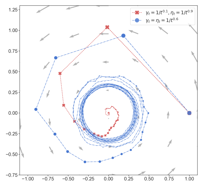
Figure 1: Behavior of (EG) and (DSEG) on Problem (2) with Gaussian oracle noise. Even with a vanishing, square-summable stepsize $\gamma_{t}=1/t^{0.6}$, the iterates of (EG) cycle; in contrast, (DSEG) with $\gamma_{t}=1/t^{0.1}$ and $\eta_{t}=1/t^{0.9}$ converges.

Figure 2: The stepsize exponents allowed by Assumption 4 for convergence (shaded green). Dashed lines are strict frontiers. Note that vanilla EG (the separatrix $r_{\gamma}=r_{\eta}$) passes just outside of this region, explaining the method’s failure.

4 Extragradient with stepsize scaling

At a high level, Proposition 1 suggests that the benefit of the exploration step is negated by the noise as the iterates of (EG) get closer to the problem’s solution set. To rectify this issue, we will consider a more flexible, DSEG (DSEG) method of the form

$$X_{t+\frac{1}{2}}=X_{t}-\gamma_{t}\hat{V}_{t},\quad\quad X_{t+1}=X_{t}-\eta_{t}\hat{V}_{t+\frac{1}{2}},$$ (DSEG)

with $\gamma_{t}\geq\eta_{t}>0$. The key idea in (DSEG) is that the scaling of the method’s stepsize parameters affords us an extra degree of freedom which can be tuned to order. In particular, motivated by the failure of (EG) described in the previous section, we will take a stepsize scaling schedule in which the exploration step evolves at a more aggressive time-scale compared to the update step. In so doing, the method will keep exploring (possibly with a near-constant stepsize) while maintaining a cautious update policy that does not blindly react to the observed oracle signals.

For illustration and comparison, we plot in Fig. 2 an instance of this method with a fairly aggressive exploration schedule and a respectively conservative update policy. In contrast to (EG), the iterates of (DSEG) now converge to a solution. We encode this as a positive counterpart to Proposition 1 below:

Proposition 1^′.

Suppose that (DSEG) is run on the problem (2) with oracle feedback $\hat{V}_{t}=V(\theta_{t},\phi_{t})+(\xi_{t},0)$ for some zero-mean random variable $\xi_{t}$ with variance $\sigma^{2}>0$. If the method’s stepsize policies are of the form $\gamma_{t}=1/t^{r_{\gamma}}$ and $\eta_{t}=1/t^{r_{\eta}}$ for some $r_{\eta}>r_{\gamma}\geq 0$ with $r_{\gamma}+r_{\eta}\leq 1$, we have $\lim_{t\to\infty}\operatorname{\mathbb{E}}[\theta_{t}^{2}+\phi_{t}^{2}]\to 0$.

From an analytic viewpoint, what distinguishes (EG) from (DSEG) is the following refined bound:

Lemma 1.

Under Assumptions 1 and 2, for all $t=1,2,\dotsc$ and all $x^{\star}\in\mathcal{X}^{\star}$, it holds

$$\operatorname{\mathbb{E}}[\lVert X_{t+1}-x^{\star}\rVert^{2}\nonscript\>|\nonscript\>\mathopen{}\mathcal{F}_{t}] \leq(1+C_{t}\operatorname{\kappa}^{2})\lVert X_{t}-x^{\star}\rVert^{2}-2\eta_{t}\operatorname{\mathbb{E}}[\langle V(X_{t+\frac{1}{2}}),X_{t+\frac{1}{2}}-x^{\star}\rangle\nonscript\>|\nonscript\>\mathopen{}\mathcal{F}_{t}]$$

$$-\gamma_{t}\eta_{t}(1-\gamma_{t}^{2}\beta^{2}-8\gamma_{t}\eta_{t}\operatorname{\kappa}^{2})\lVert V(X_{t})\rVert^{2}+C_{t}\sigma^{2},$$ (3)

with constant $C_{t}=4\gamma_{t}^{2}\eta_{t}\beta+2\gamma_{t}^{3}\eta_{t}\beta^{2}+4\eta_{t}^{2}+16\gamma_{t}^{2}\eta_{t}^{2}\operatorname{\kappa}^{2}$.

The proof of Lemma 1, which we defer to the supplement, relies on a careful analysis of the update between successive iterates to separate the deterministic and the stochastic effects. Analyzing the bound of Lemma 1 term-by-term gives a clear picture of how an aggressive exploration stepsize policy can be helpful:

• The term $\gamma_{t}\eta_{t}(1-\gamma_{t}^{2}\beta^{2}-8\gamma_{t}\eta_{t}\operatorname{\kappa}^{2})\lVert V(X_{t})\rVert^{2}$ provides a consistently negative contribution as long as $\sup_{t}\gamma_{t}<1/3\max(\beta,\operatorname{\kappa})$.

• The term $C_{t}$ is antagonistic and needs to be made as small as possible.

• The term $\operatorname{\mathbb{E}}[\langle V(X_{t+\frac{1}{2}}),X_{t+\frac{1}{2}}-x^{\star}\rangle\nonscript\>|\nonscript\>\mathopen{}\mathcal{F}_{t}]$ plays a lesser role since it is non-negative for variational stable problems (see upcoming Assumption 3) and is even identically zero in bilinear problems.

Therefore, to obtain convergence, one needs the coefficient $\gamma_{t}\eta_{t}$ to be as large as possible and, concurrently, each of the terms $\gamma_{t}^{2}\eta_{t}$, $\gamma_{t}^{3}\eta_{t}$, $\eta_{t}^{2}$ and $\gamma_{t}^{2}\eta_{t}^{2}$ that appear in $C_{t}$ should be as small as possible. Formally, this would lead to the requirement $\sum_{t}\gamma_{t}\eta_{t}=\infty$ and $\sum_{t}\gamma_{t}^{2}\eta_{t}+\eta_{t}^{2}<\infty$. These conditions can be simultaneously achieved by a suitable choice of $\gamma_{t}$ and $\eta_{t}$ (cf. Proposition 1^′ above), but they are mutually exclusive if $\gamma_{t}=\eta_{t}$. This observation is the key motivation for the scale separation between the exploration and the update mechanisms in (DSEG), and is the principal reason that (EG) fails to converge in bilinear problems.

5 Convergence analysis

We now proceed with our main results for the DSEG algorithm. We begin in Section 5.1 with an asymptotic convergence analysis for (DSEG); subsequently, in Section 5.2, we examine the algorithm’s rate of convergence; finally, in Section 5.3, we zero in on affine problems. Given our interest in non-monotone problems, we make a clear distinction between global results (which require global assumptions) and local ones (which apply to more general problems).

5.1 Asymptotic convergence

Global convergence.

​​Our assumption for global convergence is a variational stability condition.

Assumption 3.

The operator $V$ satisfies $\langle V(x),x-x^{\star}\rangle\geq 0$ for all $x\in\mathbb{R}^{d}$, $x^{\star}\in\mathcal{X}^{\star}$.

Assumption 3 is verified for all monotone operators but it also encompasses a wide range of non-monotone problems; for an overview see e.g., [6, 12, 15, 19, 24] and references therein.

To leverage this assumption, we will further need the algorithm’s update step to decrease sufficiently quickly relative to the corresponding exploration step. Formally (and with a fair degree of hindsight), this boils down to the following:

Assumption 4.

The stepsizes of (DSEG) satisfy $\sum_{t}\gamma_{t}\eta_{t}=\infty$,  $\sum_{t}\eta_{t}^{2}<\infty$,  and $\sum_{t}\gamma_{t}^{2}\eta_{t}<\infty$.

Assumption 4 essentially posits that $\eta_{t}/\gamma_{t}\to 0$ as $t\to\infty$, so it reflects precisely the principle of “aggressive exploration, conservative updates”. In particular, Assumption 4 rules out the choice $\gamma_{t}=\eta_{t}$ which would yield the vanilla EG algorithm, providing further evidence for the use of a double stepsize policy. A typical stepsize policy for (DSEG) is

$$\gamma_{t}=\frac{\gamma}{(t+b)^{r_{\gamma}}}~{}~{}~{}\text{ and }~{}~{}~{}\eta_{t}=\frac{\eta}{(t+b)^{r_{\eta}}}$$ (4)

for some $\gamma,\eta,b>0$ and exponents $r_{\gamma},r_{\eta}\in[0,1]$. Assumption 4 then translates as $r_{\gamma}+r_{\eta}\leq 1$, $2r_{\eta}>1$, and $2r_{\gamma}+r_{\eta}>1$ as represented in Fig. 2. With this in mind, we have the following convergence result.

Theorem 1.

Let Assumptions 1, 2, 3 and 4 hold and $\sup_{t}\gamma_{t}<1/3\max(\beta,\operatorname{\kappa})$, then the iterates $X_{t}$ of $\eqref{eq:DSEG}$ converge almost surely to a solution $x^{\star}$ of (Opt).

As far as we are aware, this is the first result of this type for stochastic first-order methods: almost sure convergence typically requires stronger hypotheses guaranteeing that $\langle V(x),x-x^{\star}\rangle$ is uniformly positive when $x\notin\mathcal{X}^{\star}$ [15, 24]. In particular, Theorem 1 implies the almost sure convergence of the algorithm for bilinear problems like (2) where EG and standard gradient methods do not converge.

Local convergence.

To extend Theorem 1 to fully non-monotone settings, we will consider the following local version of Assumptions 1, 2 and 3 near a solution point $x^{\star}$:

Assumption 1^′.

The field $V$ is $\beta$-Lipschitz continuous near $x^{\star}$, i.e., for all $x,x^{\prime}$ near $x^{\star}$,

$$\lVert V(x^{\prime})-V(x)\rVert\leq\beta\lVert x^{\prime}-x\rVert.$$

Assumption 2^′.

Let $x^{\star}\in\mathcal{X}^{\star}$ and $U$ be a neighborhood of $x^{\star}$. The noise term $Z_{t}$ of SFO satisfies

$$a)\;\;\textit{Zero-mean:} \operatorname{\mathbb{E}}[Z_{t}\nonscript\>|\nonscript\>\mathopen{}\mathcal{F}_{t}]\operatorname{\mathds{1}}_{\{X_{t}\in U\}}=0.\hskip 170.00026pt$$ (5a)

$$b)\;\;\textit{Moment control:} \operatorname{\mathbb{E}}[\lVert Z_{t}\rVert^{q}\nonscript\>|\nonscript\>\mathopen{}\mathcal{F}_{t}]\operatorname{\mathds{1}}_{\{X_{t}\in U\}}\leq(\sigma+\operatorname{\kappa}\lVert X_{t}-x^{\star}\rVert)^{q}.$$ (5b)

for some $q>2$ and $\sigma,\operatorname{\kappa}\geq 0$.

Assumption 3^′.

The operator $V$ satisfies $\langle V(x),x-x^{\star}\rangle\geq 0$ for all $x$ near $x^{\star}$.

Notice that (5b) is slightly stronger than (1b) in the sense that we now require to control the $q^{th}$ moment of the noise for some $q>2$. Nonetheless, this condition as well as the unbiasedness assumption only need to be satisfied in a neighborhood of $x^{\star}$. Our next result shows that, with these modified assumptions, the DSEG algorithm converges locally to solutions with high probability:

Theorem 2.

Fix a tolerance level $\delta>0$ and suppose that Assumptions 1^′, 2^′ and 3^′ hold for some isolated solution $x^{\star}$ of (Opt). Assume further that (DSEG) is run with stepsize parameters of the form (4) with small enough $\gamma$, $\eta$ and proper choice of $r_{\gamma},r_{\eta}$ (cf. Fig. 2). If the algorithm is not initialized too far from $x^{\star}$, its iterates converge to $x^{\star}$ with probability at least $1-\delta$.

The first step towards proving Theorem 2 is to show that the generated iterates stay close to $x^{\star}$ with arbitrarily high probability. To achieve this, one needs to control the total noise accumulating from each noisy step, a task which is made difficult by the fact that the norm of the SFO feedback can only be upper bounded recursively and thus depends on previous iterates. In the supplement, we dedicate a lemma to the study of such recursive stochastic processes, and we build our analysis on this lemma.

5.2 Convergence rates

Global rate.

To study the algorithm’s convergence rate, we will require the following error bound condition:

Assumption 3^′.

For some $\tau>0$ and all $x\in\mathbb{R}^{d}$, we have

$$\lVert V(x)\rVert\geq\tau\operatorname{dist}(x,\mathcal{X}^{\star}).$$ (EB)

This kind of error bound is standard in the literature on VI for deriving last iterate convergence rates [see e.g., 21, 41, 6, 40, 22]. In particular, Assumption 3^′ is satisfied by

1. Strongly monotone operators: here, $\tau$ is the strong monotonicity modulus.

2. Affine operators: for $V(x)=Mx+v$ where $M$ is a matrix of size $d\times d$ and $v$ is a $d$-dimensional vector, $\tau$ is the minimum non-zero singular value of $M$.

In this sense, Assumption 3^′ provides a unified umbrella for two types of problems that are typically considered to be poles apart. Our first result in this context is as follows:

Theorem 3.

Suppose that Assumptions 1, 2, 3 and 3^′ hold and assume that $\gamma_{t}\leq c/\beta$ with $c<1$. Then:

1. If (DSEG) is run with $\gamma_{t}\equiv\gamma$, $\eta_{t}\equiv\eta$, we have:

   $$\operatorname{\mathbb{E}}[\operatorname{dist}(X_{t},\mathcal{X}^{\star})^{2}]\leq(1-\Delta)^{t-1}\operatorname{dist}(X_{1},\mathcal{X}^{\star})^{2}+\frac{C}{\Delta}$$

   with constants $C=(2\gamma^{2}\eta\beta+\gamma^{3}\eta\beta^{2}+\eta^{2})\sigma^{2}$ and $\Delta=\gamma\eta\tau^{2}(1-c^{2})$.

2. If (DSEG) is run with $\gamma_{t}=\gamma/(t+b)^{1-\nu}$ and $\eta_{t}=\eta/(t+b)^{\nu}$ for some $\nu\in(1/2,1)$, we have:

   $$\operatorname{\mathbb{E}}[\operatorname{dist}(X_{t},\mathcal{X}^{\star})^{2}]\leq\frac{C}{\Delta-r}\frac{1}{t^{r}}+o\left(\frac{1}{t^{r}}\right)$$

   where $r=\min(1-\nu,2\nu-1)$ and we further assume that $\gamma\eta\tau^{2}(1-c^{2})>r$. In particular, the optimal rate is attained when $\nu=2/3$, which gives $\operatorname{\mathbb{E}}[\operatorname{dist}(X_{t},\mathcal{X}^{\star})^{2}]=\operatorname{\mathcal{O}}(1/t^{1/3})$.

The first part of Theorem 3 shows that, if (DSEG) is run with constant stepsizes, the initial condition is forgotten exponentially fast and the iterates converge to a neighborhood of $\mathcal{X}^{\star}$ (though, in line with previous results, convergence cannot be achieved in this case). To make this neighborhood small, we need to decrease both $\gamma$ and $\eta/\gamma$; this would be impossible for vanilla (EG) for which $\eta/\gamma=1$.

The second part of Theorem 3 provides an $\operatorname{\mathcal{O}}(1/t^{1/3})$ last-iterate convergence rate. In Section 5.3, we further improve this rate to $\operatorname{\mathcal{O}}(1/t)$ for affine operators by exploiting their particular structure.

Local rate.

To study the algorithm’s local rate of convergence, we will focus on solutions of (Opt) that satisfy the following Jacobian regularity condition:

Assumption 3^′′.

$V$ is differentiable at $x^{\star}$ and its Jacobian matrix $\operatorname{Jac}_{V}(x^{\star})$ is invertible.

The link between Assumptions 3^′ and 3^′′ is provided by the following proposition:

Proposition 2.

If a solution $x^{\star}$ satisfies Assumption 3^′′, it satisfies (EB) in a neighborhood of $x^{\star}$.

The proof of Proposition 2 follows by performing a Taylor expansion of $V$ and invoking the minimax characterization of the singular values of a matrix; we give the details in the supplement. For our purposes, what is more important is that (EB) has now been reduced to a pointwise condition; under this much lighter requirement, we have:

Theorem 4.

Fix a tolerance level $\delta>0$ and suppose that Assumptions 1^′, 2^′ and 3^′ and 3^′′ hold for some isolated solution $x^{\star}$ of (Opt) with $q>3$. Assume further $x^{\star}$ satisfies Assumption 3^′′ and (DSEG) is run with stepsize parameters of the form $\gamma_{t}=\gamma/(t+b)^{1/3}$ and $\eta_{t}=\eta/(t+b)^{2/3}$ with large enough $b,\eta>0$. Then, there exist neighborhoods $U$, $U^{\prime}$ of $x^{\star}$ and an event $E_{U}$ such that:

1. $\operatorname{\mathbb{P}}(E_{U}\nonscript\>|\nonscript\>\mathopen{}X_{1}\in U)\geq 1-\delta$.

2. $\operatorname{\mathbb{P}}(X_{t}\in U^{\prime}\;\text{for all $t$}\nonscript\>|\nonscript\>\mathopen{}E_{U})=1$.

3. $\operatorname{\mathbb{E}}[\lVert X_{t}-x^{\star}\rVert^{2}\nonscript\>|\nonscript\>\mathopen{}E_{U}]=\operatorname{\mathcal{O}}\left(1/t^{1/3}\right)$

In words, if (DSEG) is not initialized too far from $x^{\star}$, the iterates $X_{t}$ remain close to $x^{\star}$ with probability at least $1-\delta$ and, conditioned on this event, $X_{t}$ converges to $x^{\star}$ at a rate $\operatorname{\mathcal{O}}(1/t^{1/3})$ in mean square error.

Taken together, Theorems 1 and 4 show that for all monotone stochastic problems with a non-degenerate critical point, employing the suggested stepsize policy yields an asymptotic $\operatorname{\mathcal{O}}(1/t^{1/3})$ rate. In more detail, the last point of Theorem 4 shows that, with the same kind of stepsizes as in the second part of Theorem 3, we can retrieve a $\operatorname{\mathcal{O}}(1/t^{1/3})$ convergence rate provided that the iterates stay close to the solution. Note that this rate is not a localization of Theorem 3 because, after conditioning, the unbiasedness of the noise is not guaranteed. To overcome this issue, our proof draws inspiration from Hsieh et al. [11] but the use of double stepsizes requires a much more intricate analysis which is reflected in the stronger noise assumption.

5.3 A case study of affine operators

We terminate our analysis with a dedicated treatment of affine operators which are commonly studied as a first step to understand the training of GANs [5, 9, 25, 18, 43, 1]. The following result improves the $\operatorname{\mathcal{O}}(1/t^{1/3})$ rate of Theorem 3 to $\operatorname{\mathcal{O}}(1/t)$ for affine operators.

Theorem 5.

Let $V$ be an affine operator satisfying Assumption 3, and suppose that Assumption 2 holds. Take a constant exploration stepsize $\gamma_{t}\equiv\gamma\leq c/\beta$ with $c<1$ (here $\beta$ is the largest singular value of the associated matrix). Then, the iterates $(X_{t})_{t\in\mathbb{N}}$ of (DSEG) enjoy the following rates:

1. If the update stepsize is constant $\eta_{t}\equiv\eta\leq\gamma$, then:

   $$\operatorname{\mathbb{E}}[\operatorname{dist}(X_{t},\mathcal{X}^{\star})^{2}]\leq(1-\Delta)^{t-1}\operatorname{dist}(X_{1},\mathcal{X}^{\star})^{2}+\frac{C}{\Delta}$$

   with $C=\eta^{2}(1+c^{2})\sigma^{2}$ and $\Delta=\gamma\eta\tau^{2}(1-c^{2})$.

2. If the update stepsize is of the form $\eta_{t}=\eta/(t+b)$ for $\eta>1/(\tau^{2}\gamma(1-c^{2}))$ and $b>\eta/\gamma$, then:

   $$\operatorname{\mathbb{E}}[\operatorname{dist}(X_{t},\mathcal{X}^{\star})^{2}]\leq\frac{C}{\Delta-1}\frac{1}{t}+o\left(\frac{1}{t}\right).$$

The proof of this theorem relies on the derivation of another descent lemma similar to Lemma 1 but tailored to affine operators. Note also that Assumptions 1 and 3^′ are automatically verified in this case.

Theorem 5 mirrors Theorem 3; however, in Part 1 of Theorem 5, the final precision is only determined by $\sigma^{2}$ and $\eta/\gamma$. Thus, compared to Theorem 3, there is no need to decrease $\gamma$ to obtain an arbitrarily high accuracy solution. The weaker dependence on $\gamma$ is further confirmed by Part 2, which shows a $\operatorname{\mathcal{O}}(1/t)$ rate with $\gamma_{t}$ constant. As far as we are aware, this result gives the best convergence rate for stochastic affine operators compared to the literature, and it gives yet another motivation for the use of a double stepsize strategy.

6 Numerical experiments

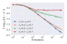
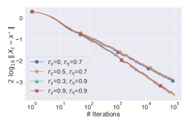
Figure 3: Convergence of a (DSEG) scheme in stochastic bilinear (left), strongly convex-concave (middle) and non convex-concave linear quadratic Gaussian GAN (right) problems. All curves are averaged over $10$ runs with the shaded area indicating the standard deviation. The benefit of aggressive exploration is evident.

This section investigates numerically the benefits of double stepsizes. We run (DSEG) with stepsize of the form (4) on three different problems: i) a bilinear zero-sum game, ii) a strongly convex-concave game and iii) a non convex-concave linear quadratic Gaussian GAN model [5, 28]. We examine their behavior when $r_{\gamma}$ and $r_{\eta}$ vary. The exact description of the problems and the experimental details are deferred to the supplement.

As shown in Fig. 3, for bilinear game and Gaussian GAN examples, choosing $r_{\eta}<r_{\gamma}$ turns out to be necessary for the convergence of the algorithm, and the convergence speed is positively related to the difference $r_{\gamma}-r_{\eta}$, as per our analysis. For a strongly convex-concave problem, it is known that the iterates produced by (EG) with noisy feedback achieve $\operatorname{\mathcal{O}}(1/t)$ convergence for proper choice of $(\gamma_{t})_{t\in\mathbb{N}}$ [15, 11]. Our experiment moreover reveals that when a double step-size policy is considered, the convergence speed of the algorithm seems to only depend on $(\eta_{t})_{t\in\mathbb{N}}$ and using aggressive $(\gamma_{t})_{t\in\mathbb{N}}$ has little influence, if any, suggesting that taking a larger exploration step may be a universal solution. Going one step further, we conduct experiments and observe similar phenomena for the generalized OG method [27, 38] when the output vector is appropriately chosen. We refer the interested reader to the supplement for a dedicated discussion.

7 Conclusion

In this paper, we examined the benefits of employing a DSEG method for which the exploration step is more aggressive than the update step. This additional flexibility turns out to be both necessary and sufficient for the method to achieve superior convergence properties relative to vanilla stochastic EG methods in a large spectrum of problems including bilinear games and some non convex-concave models.

Our results constitute a first attempt towards designing an algorithm that provably avoids cycles and similar non-convergent phenomena in a fully stochastic setting. Several interesting future directions include an extended analysis with relaxation of the variational stability assumption as well as the design of a fully adaptive and/or universal method on the basis of our results.

Broader impact

This work does not present any foreseeable societal consequence.

Appendix A Additional related work

The first analysis of EG (EG) with stochastic feedback traces back to the work of Juditsky et al. [14], where a $\operatorname{\mathcal{O}}(1/\sqrt{t})$ ergodic convergence was shown for monotone problems, and this rate is known to be optimal without further assumptions [30]. Since then, a large number of works have been dedicated to studying the convergence behavior of stochastic EG-type algorithms, either for better understanding of the algorithm itself or in the hope of finding a better way to incorporate EG with stochasticity.

Almost sure convergence of stochastic EG was first investigated in Kannan & Shanbhag [15]. In the said paper, almost convergence was shown for pseudomonotone plus operators and by additionally assuming that the map is strongly pseudomonotone or monotone and weak-sharp, the authors managed to prove a $\operatorname{\mathcal{O}}(1/{t})$ convergence of the iterate produced by the algorithm. In [24], the pseudo-monotonicity-plus assumption is relaxed to show that stochastic EG still enjoys last-iterate convergence in strict coherent problems. Nonetheless, these results fail to justify the use of EG for stochastic monotone problems, as illustrated in Section 3. Therefore, to improve the convergence behavior of EG in stochastic problems, several modifications to the original stochastic EG have been proposed [2, 12, 26]. In addition to the ones discussed in Section 1, Mishchenko et al. [26] advocated a repeated sampling strategy and illustrated numerically its better performance when applied to GAN training. They also showed that their proposed algorithm retain the same convergence guarantee as traditional stochastic EG.

In order to reduce the overall computational cost, another line of research aims at designing optimization methods that solve variational problems with a single oracle call per iteration (instead of the two in EG). Algorithms of this family include for example OG (OG) [5] and PEG (PEG) [9, 36]. See Hsieh et al. [11] for a recent overview and corresponding treatment in the stochastic setting. Very recently, the convergence of stochastic OG (OG) are further improved in two different ways. In [7], the authors introduced a multistage version of OG for stochastic strongly monotone problems to optimize the dependence of convergence speed on initial error and noise characteristics. On the other hand, inspired by the success of adaptive methods in deep learning, Liu et al. [19] designed an adaptive variant of OG and showed that it enjoyed an adaptive complexity that varies according to the growth rate of the cumulative stochastic gradient. To complete the list, also in the goal of reducing overall computation though under a quite different perspective, Jelassi et al. [13] analyzed a randomized version of stochastic EG in multiplayer game to make the extrapolation step amenable to massive multiplayer settings.

Appendix B Generalized optimistic gradient

Considering the similarity between EG and its single-call variants, we believe our analysis on (DSEG) also suggests essential modifications in terms of stepsizes that should be carried out for these algorithms in the face of stochasticity. As an example, we investigate the OG method of Daskalakis et al. [5], and find out that some surprising conclusions can be drawn after applying the double stepsize rule. The generalized OG recursion is commonly stated as follows [27, 38]:

$$X_{t+1}=X_{t}-\eta_{t}\hat{V}_{t}-\gamma_{t}(\hat{V}_{t}-\hat{V}_{t-1})$$ (OG)

where $\gamma_{t}$ is sometimes called the optimism rate. Similarly to our conclusions, it has been empirically observed that taking large optimism rate often yields better convergence in stochastic problems [33].

Hsieh et al. [11] pointed out that OG is equivalent to the modified Arrow-Hurwitz method introduced by Popov [36] and also referred to as PEG (PEG) by Gidel et al. [9]. Using a double stepsize policy, PEG becomes:

$$X_{t+\frac{1}{2}}=X_{t}-\gamma_{t}\hat{V}_{t-\frac{1}{2}},\quad X_{t+1}=X_{t}-\eta_{t}\hat{V}_{t+\frac{1}{2}}.$$ (DSPEG)

Hence, leading states can be recursively written as

$$X_{t+\frac{1}{2}}=X_{t-\frac{1}{2}}-\eta_{t-\frac{3}{2}}\hat{V}_{t-\frac{1}{2}}-\gamma_{t-\frac{1}{2}}\hat{V}_{t-\frac{1}{2}}+\gamma_{t-\frac{3}{2}}\hat{V}_{t-\frac{3}{2}}.$$

We thereby see that (OG) and (DSPEG) are almost equivalent and they mostly differ in the choice of vectors that the method outputs at the end: OG suggests outputting $X_{t}$ while PEG instead looks at $X_{t}+\gamma_{t-1}\hat{V}_{t-1}$. This nuance turns out to be of importance when generalized OG is applied to stochastic problems. By analogy with our analysis for (DSEG), we reasonably conjecture that taking $\eta_{t}<\gamma_{t}$ guarantees the convergence of $X_{t}+\gamma_{t-1}\hat{V}_{t-1}$, and this may occur even if $\gamma_{t}$ is set to constant. Nonetheless, this also implies that if the noise is not vanishing at the solution, $X_{t}$, which corresponds to the exploration state in PEG, might exhibit much slower convergence or even not converge at all.

To summarize, when running (OG) for stochastic problems, we should look at the residual iterate $X_{t}+\gamma_{t-1}\hat{V}_{t-1}$ instead of the optimistic iterate $X_{t}$. Interestingly, this conclusion is consistent with the ODE analysis of OG by Ryu et al. [38], and explains some experimental results of said work. Furthermore, taking an aggressive exploration step $\gamma_{t}$ and a more conservative update step $\eta_{t}$ may be very beneficial both in theory (for the last iterate convergence and rate) and in practice as confirmed by our experiments just below.

Appendix C Experimental details and additional experiments

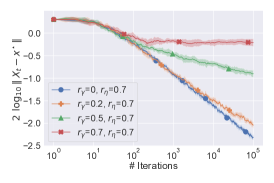
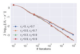
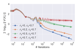
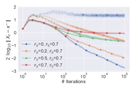
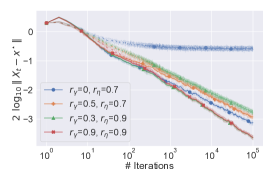
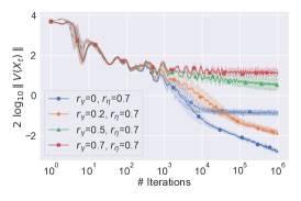
Figure 4: Convergence of (DSEG) (top) and (OG) (bottom) schemes in stochastic bilinear (left), strongly convex-concave (middle) and non convex-concave covariance matrix learning (right) problems. In the second row the dashed lines and the solid lines depict respectively the results for optimistic iterates and residual iterates. We observe clearly the benefit of (i) aggressive exploration and (ii) using residual iterates in generalized OG methods. All curves are averaged over $10$ runs with the shaded area indicating the standard deviation.

We provide here a detailed explanation of the problems that we consider in our experiments and elucidate the used parameters. Additional experimental results are also presented.

Bilinear zero-sum games.

The bilinear zero-sum game takes the form

$$\mathcal{L}(\theta,\phi)=\theta^{\top}\!C\phi$$

where $C$ is a $50\times 50$ invertible matrix in our experiment; in that case, $(\theta^{\star},\phi^{\star})=(0,0)$ is the only equilibrium point. We simulate the stochastic oracle by adding a Gaussian noise $Z\sim\mathcal{N}(0,\sigma I)$ with $\sigma=0.5$ to the vector field.

Strongly convex-concave game.

To understand the effect of aggressive exploration in strongly convex-concave problems, we inspect the following example

$$\mathcal{L}(\theta,\phi)=\big{(}\theta^{\top}\!A_{2}\theta\big{)}^{2}+2\theta^{\top}\!A_{1}\theta+4\theta^{\top}\!C\phi-2\phi^{\top}\!B_{1}\phi-\big{(}\phi^{\top}\!B_{2}\phi\big{)}^{2},$$

where $A_{1}$, $A_{2}$, $B_{1}$, $B_{2}$ are $50\times 50$ positive definite matrices so $(\theta^{\star},\phi^{\star})=(0,0)$ is again the only solution of the problem. We take the same noise distribution to construct the stochastic oracle.

Linear Quadratic Gaussian GAN.

Finally, to examine the convergence of (DSEG) in stochastic non convex-concave problems, we consider the following problem from Daskalakis et al. [5] and Nagarajan & Kolter [28]:

$$\mathcal{L}(Y,W)=\operatorname{\mathbb{E}}_{x\sim\mathcal{N}(0,\Sigma)}[x^{\top}\!Wx]-\operatorname{\mathbb{E}}_{z\sim\mathcal{N}(0,I)}[z^{\top}\!Y^{\top}\!WYz].$$

This saddle-point problem corresponds to the WGAN formulation without clipping when data are sampled from a normal distribution with covariance matrix $\Sigma$, i.e., $x\sim\mathcal{N}(0,\Sigma)$, and the generator and the discriminator are respectively defined by $G(z)=Yz$, $D(x)=x^{\top}\!Wx$. The stochasticity is induced by the sampling of $x$ and $z$. For the experiments we take a mini-batch of size $128$ and $x$ and $z$ of dimension $10$. As the game may possess multiple equilibria, the squared norm of $V$ is traced as the convergence measure.

	Double stepsize extragradient (DSEG)			Generalized optimistic gradient (OG)
	$\gamma_{1}$	$\eta_{1}$	$b$	$\gamma_{1}$	$\eta_{1}$	$b$
Bilinear	1	0.1	19	0.5	0.05	19
Strongly convex-concave	0.1	0.05	19	0.1	0.05	19
Gaussian GAN	0.5	0.05	49	0.05	0.025	99

Table 2: The stepsize parameters for (DSEG) and (OG) in the experiments.

Results for (DSEG) and (OG).

Following the discussion of Appendix B, we complement the illustration of our method (DSEG) by a comparison with (OG) with properly chosen outputs. In the experiments, both (DSEG) and (OG) are run with stepsize of the form (4) with various $r_{\gamma}$ and $r_{\eta}$. In order to start with the same value for different exponents, we fix $b,\gamma_{1},$ and $\eta_{1}$ as indicated in Table 2, from which we deduce $\gamma=\gamma_{1}(1+b)^{r_{\gamma}}$ and $\eta=\eta_{1}(1+b)^{r_{\eta}}$.

As shown in Fig. 4, for bilinear game and Gaussian GAN examples, the convergence speed of (DSEG) is positively related to the difference $r_{\gamma}-r_{\eta}$, as per our analysis. For the strongly convex-concave problem, the vanilla (EG) already achieves $\operatorname{\mathcal{O}}(1/t)$ convergence, and the plot shows that using aggressive $(\gamma_{t})_{t\in\mathbb{N}}$ has little influence on it.

Regarding (OG) with the residual iterates, the algorithm has roughly the same convergence behavior as for (DSEG). In contrast, the optimistic iterates tend to converge much slower. In particular, choosing a constant exploration step gives the fastest convergence of the residual iterate though the optimistic iterate does not converge, in line with our discussion in Appendix B.

Additional discussions for bilinear games.

Few algorithms provably converge in stochastic bilinear games, and among them there are SHGD (SHGD) [20] and gradient descent with anchoring [38]. In Fig. 5 we illustrate the convergences of DSEG and these two algorithms for the stochastic bilinear saddle-point example. For (DSEG) we adopt the optimal stepsize schedule as described in Theorem 5-2. The leading stepsize is set to constant $\gamma_{t}\equiv 1$ and the update stepsize is $\eta_{t}=\eta/(t+b)$ with $\eta=2$ and $b=19$. The same $(\eta_{t})_{t\in\mathbb{N}}$ is also used as the stepsize of SHGD, in accordance with the decreasing stepsize strategy presented in [20]. As for the anchored gradient methods, its update is written as

$$X_{t+1}=X_{t}-\frac{1-r}{t^{r}}+\frac{(1-r)\gamma}{t^{\nu}}(X_{1}-X_{t}),$$

and it is proved to converge in all stochastic monotone problems for $\gamma>0$ and $r,\nu\in(1/2,1)$. Since no explicit rate is proven for this algorithm when stochastic gradients are used,

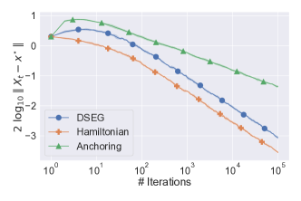
Figure 5: Comparison of DSEG, stochastic Hamiltonian gradient descent and anchored gradient in the stochastic bilinear example. All curves are averaged over $10$ runs with the shaded area indicating the standard deviation.

we run hyperparameter optimization to search for the best $\gamma,r$ and $\nu$, and end up with $\gamma=1,r=0.7,\nu=0.9$.

Fig. 5 confirms that asymptotically both DSEG and SHGD converge in $\operatorname{\mathcal{O}}(1/t)$ as predicted by the theory. SHGD converges slightly faster than DSEG for the first few iterations as it circumvents the rotational dynamics by directly performing stochastic gradient descent on $\lVert V(\cdot)\rVert^{2}$, which turns out to be a positive definite quadratic form when $V$ is linear. This however comes at the cost of the use of second-order information. In fact, SHGD requires access to an unbiased estimator of $\operatorname{Jac}_{V}^{\top}V$ at every iteration. Finally, anchoring converges much slower compared to these two methods. Without further theoretical investigation we do not know if this kind of algorithms can achieve the same $\operatorname{\mathcal{O}}(1/t)$ convergence rate in this problem.

Appendix D Technical lemmas

In this section we recall several important lemmas that are frequently used in the analysis of stochastic iterative methods. The first three lemmas on numerical sequences are useful for deriving convergence rates of the algorithms. See e.g., Polyak [35] for an abundance of results of this type.

Lemma D.1.

Let $(a_{t})_{t\in\mathbb{N}}$ be a sequence of real numbers such that for all $t$,

$$a_{t+1}\leq(1-q)a_{t}+q^{\prime},$$

where $1>q>0$ and $q^{\prime}>0$. Then,

$$a_{t}\leq(1-q)^{t-1}a_{1}+\frac{q^{\prime}}{q}.$$

The above lemma comes into play when an algorithm is run with constant stepsize sequences, whereas we resort to the following two lemmas in case of decreasing stepsize sequences of the form (4).

Lemma D.2 (Chung [4, Lemma 1]).

Let $(a_{t})_{t\in\mathbb{N}}$ be a sequence of real numbers and $b\in\mathbb{N}$ such that for all $t$,

$$a_{t+1}\leq\left(1-\frac{q}{t+b}\right)a_{t}+\frac{q^{\prime}}{(t+b)^{r+1}},$$

where $q>r>0$ and $q^{\prime}>0$. Then,

$$a_{t}\leq\frac{q^{\prime}}{q-r}\frac{1}{t^{r}}+o\left(\frac{1}{t^{r}}\right).$$

Lemma D.3 (Chung [4, Lemma 4]).

Let $(a_{t})_{t\in\mathbb{N}}$ be a sequence of real numbers and $b\in\mathbb{N}$ such that for all $t$,

$$a_{t+1}\leq\left(1-\frac{q}{(t+b)^{\nu}}\right)a_{t}+\frac{q^{\prime}}{(t+b)^{r+\nu}},$$

where $1>\nu>0$ and $r,q,q^{\prime}>0$. Then,

$$a_{t}=\operatorname{\mathcal{O}}\left(\frac{1}{t^{r}}\right).$$

To establish almost sure convergence of the iterates, we rely on the Robbins–Siegmund theorem which apply to non-negative almost-supermatingales.

Lemma D.4 (Robbins & Siegmund [37]).

Consider a filtration $(\mathcal{F}_{t})_{t\in\mathbb{N}}$ and four non-negative $(\mathcal{F}_{t})_{t\in\mathbb{N}}$-adapted processes $(U_{t})_{t\in\mathbb{N}}$, $(\lambda_{t})_{t\in\mathbb{N}}$, $(\chi_{t})_{t\in\mathbb{N}}$, $(\zeta_{t})_{t\in\mathbb{N}}$ such that $\sum_{t}\lambda_{t}<\infty$ and $\sum_{t}\chi_{t}<\infty$ with probability one and $\forall t\in\mathbb{N}$,

$$\operatorname{\mathbb{E}}[U_{t+1}\nonscript\>|\nonscript\>\mathopen{}{\mathcal{F}_{t}}]\leq(1+\lambda_{t})U_{t}+\chi_{t}-\zeta_{t}.$$ (D.1)

Then $(U_{t})_{t\in\mathbb{N}}$ converges almost surely to a random variable $U_{\infty}$ and $\sum_{t}\zeta_{t}<\infty$ almost surely.

Appendix E Proofs for global convergence results

We then start with the proofs of the global results to highlight the effect of double stepsize, before tackling the more challenging local convergence analysis.

E.1 Proof of Proposition 1: failure of stochastic extragradient

See 1

Proof.

We write the updates of the algorithm

$$\left\{\begin{array}[]{l}\theta_{t+\frac{1}{2}}=\theta_{t}-\gamma_{t}\phi_{t}-\gamma_{t}\xi_{t}\\ \phi_{t+\frac{1}{2}}=\phi_{t}+\gamma_{t}\theta_{t}\end{array}\right.~{}~{}~{}~{}~{}~{}~{}~{}\left\{\begin{array}[]{l}\theta_{t+1}=\theta_{t}-\gamma_{t}\phi_{t}-\gamma_{t}^{2}\theta_{t}-\gamma_{t}\xi_{t+\frac{1}{2}}\\ \phi_{t+1}=\phi_{t}+\gamma_{t}\theta_{t}-\gamma_{t}^{2}\phi_{t}-\gamma_{t}^{2}\xi_{t}\end{array}\right.$$

Therefore

$$\theta_{t+1}^{2}+\phi_{t+1}^{2} =(1-\gamma_{t}^{2}+\gamma_{t}^{4})(\theta_{t}^{2}+\phi_{t}^{2})+\gamma_{t}^{2}\xi_{t+\frac{1}{2}}^{2}+\gamma_{t}^{4}\xi_{t}^{2}$$

$$~{}~{}-2\gamma_{t}\xi_{t+\frac{1}{2}}((1-\gamma_{t}^{2})\theta_{t}-\gamma_{t}\phi_{t})-2\gamma_{t}^{2}\xi_{t}((1-\gamma_{t}^{2})\phi_{t}+\gamma_{t}\theta_{t}).$$

Taking expectation leads to

$$\operatorname{\mathbb{E}}[\theta_{t+1}^{2}+\phi_{t+1}^{2}]=(1-\gamma_{t}^{2}+\gamma_{t}^{4})\operatorname{\mathbb{E}}[\theta_{t}^{2}+\phi_{t}^{2}]+(\gamma_{t}^{2}+\gamma_{t}^{4})\sigma^{2}.$$

For sake of simplicity, let us denote $a_{t}=\operatorname{\mathbb{E}}[\theta_{t}^{2}+\phi_{t}^{2}]$. We consider two scenarios:

Case 1: $\gamma_{t}^{2}\geq 1$. We have $1-\gamma_{t}^{2}+\gamma_{t}^{4}\geq 1$ and consequently $a_{t+1}\geq a_{t}$.

Case 2: $\gamma_{t}^{2}<1$. Notice that

$$a_{t+1}-\frac{(1+\gamma_{t}^{2})\sigma^{2}}{1-\gamma_{t}^{2}}=(1-\gamma_{t}^{2}+\gamma_{t}^{4})\left(a_{t}-\frac{(1+\gamma_{t}^{2})\sigma^{2}}{1-\gamma_{t}^{2}}\right).$$

We then set $\nu_{t}=(1+\gamma_{t}^{2})/(1-\gamma_{t}^{2})$. Since $1-\gamma_{t}^{2}+\gamma_{t}^{4}<1$, $a_{t+1}$ gets closer to $\nu_{t}\sigma^{2}$ than $a_{t}$. In particular, if $a_{t}<\nu_{t}\sigma^{2}$, we have $a_{t}<a_{t+1}<\nu_{t}\sigma^{2}$; otherwise, $a_{t}\geq a_{t+1}\geq\nu_{t}\sigma^{2}$. As $\nu_{t}\geq 1$, the above implies $a_{t+1}\geq\min(a_{t},\nu_{t}\sigma^{2})\geq\min(a_{t},\sigma^{2})$.

To conclude, in the two cases we have $a_{t+1}\geq\min(a_{t},\sigma^{2})$, showing $\liminf_{t\to\infty}\operatorname{\mathbb{E}}[\theta_{t}^{2}+\phi_{t}^{2}]>0$.

A remedy with double stepsize extragradient.

With different stepsizes, the updates of the algorithm write

$$\left\{\begin{array}[]{l}\theta_{t+\frac{1}{2}}=\theta_{t}-\gamma_{t}\phi_{t}-\gamma_{t}\xi_{t}\\ \phi_{t+\frac{1}{2}}=\phi_{t}+\gamma_{t}\theta_{t}\end{array}\right.~{}~{}~{}~{}~{}~{}~{}~{}\left\{\begin{array}[]{l}\theta_{t+1}=\theta_{t}-\eta_{t}\phi_{t}-\gamma_{t}\eta_{t}\theta_{t}-\eta_{t}\xi_{t+\frac{1}{2}}\\ \phi_{t+1}=\phi_{t}+\eta_{t}\theta_{t}-\gamma_{t}\eta_{t}\phi_{t}-\gamma_{t}\eta_{t}\xi_{t}\end{array}\right.$$

This now leads to

$$\operatorname{\mathbb{E}}[\theta_{t+1}^{2}+\phi_{t+1}^{2}] =((1-\gamma_{t}\eta_{t})^{2}+\eta_{t}^{2})\operatorname{\mathbb{E}}[\theta_{t}^{2}+\phi_{t}^{2}]+(\eta_{t}^{2}+\gamma_{t}^{2}\eta_{t}^{2})\sigma^{2}$$

$$=(1-2\gamma_{t}\eta_{t}+\eta_{t}^{2}+\gamma_{t}^{2}\eta_{t}^{2})\operatorname{\mathbb{E}}[\theta_{t}^{2}+\phi_{t}^{2}]+(\eta_{t}^{2}+\gamma_{t}^{2}\eta_{t}^{2})\sigma^{2}.$$

Taking $\gamma_{t}=\frac{1}{t^{r_{\gamma}}}$ and $\eta_{t}=\frac{1}{t^{r_{\eta}}}$, we get

$$\operatorname{\mathbb{E}}[\theta_{t+1}^{2}+\phi_{t+1}^{2}] =\left(1-\frac{2}{t^{(r_{\gamma}+r_{\eta})}}+\frac{1}{{t}^{2r_{\eta}}}+\frac{1}{t^{2(r_{\gamma}+r_{\eta})}}\right)\operatorname{\mathbb{E}}[\theta_{t}^{2}+\phi_{t}^{2}]+\left(\frac{1}{{t}^{2r_{\eta}}}+\frac{1}{t^{2(r_{\gamma}+r_{\eta})}}\right)\sigma^{2}$$

$$\leq\left(1-\frac{1.5}{t^{(r_{\gamma}+r_{\eta})}}\right)\operatorname{\mathbb{E}}[\theta_{t}^{2}+\phi_{t}^{2}]+\frac{2\sigma^{2}}{{t}^{2r_{\eta}}}$$

$$=\mathcal{O}\left(\frac{1}{t^{(r_{\eta}-r_{\gamma})}}\right)$$

where the inequality comes from $1-2/t^{(r_{\gamma}+r_{\eta})}+1/{t}^{2r_{\eta}}+1/t^{2(r_{\gamma}+r_{\eta})}\leq 1-1.5/t^{(r_{\gamma}+r_{\eta})}$ for large enough $t$ and the last part is an application of either Lemma D.2 or Lemma D.3 with $q=1.5>r=r_{\eta}-r_{\gamma}>0$ (starting at large enough $t$).

Hence, $\operatorname{\mathbb{E}}[\theta_{t}^{2}+\phi_{t}^{2}]\to 0$, i.e. we can find a double stepsize choice, with an aggressive extrapolation step and a conservative update step ($r_{\gamma}<r_{\eta}$) such that $(\theta_{t},\phi_{t})\to(0,0)$ in mean squared error.
∎

E.2 Proof of Lemma 1

See 1

Proof.

Let us denote by $\operatorname{\mathbb{E}}_{t}[\cdot]=\operatorname{\mathbb{E}}[\cdot\nonscript\>|\nonscript\>\mathopen{}{\mathcal{F}_{t}}]$ the conditional expectation with respect to the filtration up to time $t$ and $\tilde{X}_{t+\frac{1}{2}}=X_{t}-\gamma_{t}V(X_{t})$ the leading state that is generated with deterministic update so that $X_{t+\frac{1}{2}}=\tilde{X}_{t+\frac{1}{2}}-\gamma_{t}Z_{t}$. We develop

$$\lVert X_{t+1}-x^{\star}\rVert^{2} =\lVert X_{t}-\eta_{t}\hat{V}_{t+\frac{1}{2}}-x^{\star}\rVert^{2}$$

$$=\lVert X_{t}-x^{\star}\rVert^{2}-2\eta_{t}\langle\hat{V}_{t+\frac{1}{2}},X_{t}-x^{\star}\rangle+\eta_{t}^{2}\lVert\hat{V}_{t+\frac{1}{2}}\rVert^{2}$$

$$=\lVert X_{t}-x^{\star}\rVert^{2}-2\eta_{t}\langle\hat{V}_{t+\frac{1}{2}},\tilde{X}_{t+\frac{1}{2}}-x^{\star}\rangle-2\gamma_{t}\eta_{t}\langle\hat{V}_{t+\frac{1}{2}},V(X_{t})\rangle+\eta_{t}^{2}\lVert\hat{V}_{t+\frac{1}{2}}\rVert^{2}.$$ (E.1)

We would then like to bound the different terms appearing on the right-hand side (RHS) of the equality. With the zero-mean assumption (1a), conditioning on $\mathcal{F}_{t}$ leads to

$$\operatorname{\mathbb{E}}_{t}[\langle\hat{V}_{t+\frac{1}{2}},\tilde{X}_{t+\frac{1}{2}}-x^{\star}\rangle] =\operatorname{\mathbb{E}}_{t}[\langle V(X_{t+\frac{1}{2}}),\tilde{X}_{t+\frac{1}{2}}-x^{\star}\rangle]$$

$$=\operatorname{\mathbb{E}}_{t}[\langle V(X_{t+\frac{1}{2}}),\tilde{X}_{t+\frac{1}{2}}-\gamma_{t}Z_{t}-x^{\star}\rangle]+\operatorname{\mathbb{E}}_{t}[\langle V(X_{t+\frac{1}{2}}),\gamma_{t}Z_{t}\rangle]$$

$$=\operatorname{\mathbb{E}}_{t}[\langle V(X_{t+\frac{1}{2}}),X_{t+\frac{1}{2}}-x^{\star}\rangle]+\gamma_{t}\operatorname{\mathbb{E}}_{t}[\langle V(X_{t+\frac{1}{2}})-V(\tilde{X}_{t+\frac{1}{2}}),Z_{t}\rangle],$$ (E.2)

where in the last line we use the fact that $V(\tilde{X}_{t+\frac{1}{2}})$ is $\mathcal{F}_{t}$-measurable so

$$\operatorname{\mathbb{E}}_{t}[\langle V(\tilde{X}_{t+\frac{1}{2}}),Z_{t}\rangle]=\langle V(\tilde{X}_{t+\frac{1}{2}}),\operatorname{\mathbb{E}}_{t}[Z_{t}]\rangle=0.$$

By Lipschitz continuity of $V$

$$-\langle V(X_{t+\frac{1}{2}})-V(\tilde{X}_{t+\frac{1}{2}}),Z_{t}\rangle\leq\lVert V(X_{t+\frac{1}{2}})-V(\tilde{X}_{t+\frac{1}{2}})\rVert\lVert Z_{t}\rVert\leq\gamma_{t}\beta\lVert Z_{t}\rVert^{2}.$$ (E.3)

On the other hand, $\operatorname{\mathbb{E}}_{t}[\langle\hat{V}_{t+\frac{1}{2}},V(X_{t})\rangle]=\operatorname{\mathbb{E}}_{t}[\langle V(X_{t+\frac{1}{2}}),V(X_{t})\rangle]$ and $\operatorname{\mathbb{E}}_{t}[\lVert\hat{V}_{t+\frac{1}{2}}\rVert^{2}]=\operatorname{\mathbb{E}}_{t}[\lVert V(X_{t+\frac{1}{2}})\rVert^{2}]+\operatorname{\mathbb{E}}_{t}[\lVert Z_{t+\frac{1}{2}}\rVert^{2}]$. By $\eta_{t}\leq\gamma_{t}$, Lipschitz continuity of $V$ and $X_{t}-X_{t+\frac{1}{2}}=\gamma_{t}\hat{V}_{t}$, we get

$$-2\gamma_{t}\eta_{t}\langle V(X_{t+\frac{1}{2}}),V(X_{t})\rangle+\eta_{t}^{2}\lVert V(X_{t+\frac{1}{2}})\rVert^{2}$$

$$~{}~{}\leq-2\gamma_{t}\eta_{t}\langle V(X_{t+\frac{1}{2}}),V(X_{t})\rangle+\gamma_{t}\eta_{t}\lVert V(X_{t+\frac{1}{2}})\rVert^{2}$$

$$~{}~{}=\gamma_{t}\eta_{t}(\lVert V(X_{t})-V(X_{t+\frac{1}{2}})\rVert^{2}-\lVert V(X_{t})\rVert^{2})$$

$$~{}~{}\leq\gamma_{t}^{3}\eta_{t}\beta^{2}\lVert\hat{V}_{t}\rVert^{2}-\gamma_{t}\eta_{t}\lVert V(X_{t})\rVert^{2},$$ (E.4)

Similar to before we may write $\operatorname{\mathbb{E}}_{t}[\lVert\hat{V}_{t}\rVert^{2}]=\operatorname{\mathbb{E}}_{t}[\lVert V(X_{t})\rVert^{2}]+\operatorname{\mathbb{E}}_{t}[\lVert Z_{t}\rVert^{2}]$. Therefore, combining (E.1), (E.2), (E.3), (E.4), we deduce the following

$$\operatorname{\mathbb{E}}_{t}[\lVert X_{t+1}-x^{\star}\rVert^{2}] \leq\lVert X_{t}-x^{\star}\rVert^{2}-2\eta_{t}\operatorname{\mathbb{E}}_{t}[\langle V(X_{t+\frac{1}{2}}),X_{t+\frac{1}{2}}-x^{\star}\rangle]-(\gamma_{t}\eta_{t}-\gamma_{t}^{3}\eta_{t}\beta^{2})\lVert V(X_{t})\rVert^{2}$$

$$~{}~{}+(2\gamma_{t}^{2}\eta_{t}\beta+\gamma_{t}^{3}\eta_{t}\beta^{2})\operatorname{\mathbb{E}}[\lVert Z_{t}\rVert^{2}]+\eta_{t}^{2}\operatorname{\mathbb{E}}[\lVert Z_{t+\frac{1}{2}}\rVert^{2}].$$ (E.5)

To finish the proof, we would like to bound the noise terms. Using (1b) and Jensen’s inequality (recall that $q\geq 2$), we have

$$\operatorname{\mathbb{E}}[\lVert Z_{t}\rVert^{2}]\leq(\sigma+\operatorname{\kappa}\lVert X_{t}-x^{\star}\rVert)^{2}\leq 2\sigma^{2}+2\operatorname{\kappa}^{2}\lVert X_{t}-x^{\star}\rVert^{2}.$$ (E.6)

Similarly,

$$\operatorname{\mathbb{E}}[\lVert Z_{t+\frac{1}{2}}\rVert^{2}] \leq 2\sigma^{2}+2\operatorname{\kappa}^{2}\lVert X_{t+\frac{1}{2}}-x^{\star}\rVert^{2}$$ (E.7)

$$\leq 2\sigma^{2}+4\operatorname{\kappa}^{2}\lVert X_{t+\frac{1}{2}}-X_{t}\rVert^{2}+4\operatorname{\kappa}^{2}\lVert X_{t}-x^{\star}\rVert^{2}$$

$$\leq 4\gamma_{t}^{2}\operatorname{\kappa}^{2}\lVert\hat{V}_{t}\rVert^{2}+4\operatorname{\kappa}^{2}\lVert X_{t}-x^{\star}\rVert^{2}+2\sigma^{2}$$

$$\leq 8\gamma_{t}^{2}\operatorname{\kappa}^{2}\lVert V(X_{t})\rVert^{2}+16\gamma_{t}^{2}\operatorname{\kappa}^{2}\sigma^{2}+16\gamma_{t}^{2}\operatorname{\kappa}^{4}\lVert X_{t}-x^{\star}\rVert^{2}+4\operatorname{\kappa}^{2}\lVert X_{t}-x^{\star}\rVert^{2}+2\sigma^{2}$$

Substituting (E.7) and (E.6) in (E.5), we obtain

$$\operatorname{\mathbb{E}}_{t}[\lVert X_{t+1}-x^{\star}\rVert^{2}] \leq(1+4\gamma_{t}^{2}\eta_{t}\beta\operatorname{\kappa}+2\gamma_{t}^{3}\eta_{t}\beta^{2}\operatorname{\kappa}+4\eta_{t}^{2}\operatorname{\kappa}^{2}+16\gamma_{t}^{2}\eta_{t}^{2}\operatorname{\kappa}^{4})\lVert X_{t}-x^{\star}\rVert^{2}$$

$$~{}~{}-2\eta_{t}\operatorname{\mathbb{E}}_{t}[\langle V(X_{t+\frac{1}{2}}),X_{t+\frac{1}{2}}-x^{\star}\rangle]$$

$$~{}~{}-(\gamma_{t}\eta_{t}-\gamma_{t}^{3}\eta_{t}\beta^{2}-8\gamma_{t}^{2}\eta_{t}^{2}\operatorname{\kappa}^{2})\lVert V(X_{t})\rVert^{2}$$

$$~{}~{}+(4\gamma_{t}^{2}\eta_{t}\beta+2\gamma_{t}^{3}\eta_{t}\beta^{2}+2\eta_{t}^{2}+16\gamma_{t}^{2}\eta_{t}^{2}\operatorname{\kappa}^{2})\sigma^{2}.$$

We recover (3) by using $2\eta_{t}^{2}\sigma^{2}\leq 4\eta_{t}^{2}\sigma^{2}$. ∎

E.3 Proof of Theorem 1

See 1

Proof.

The proof is divided into three key steps.

(1) With probability $1$, $\liminf_{t\rightarrow\infty}\lVert V(X_{t})\rVert=0$. Let $x^{\star}\in\mathcal{X}^{\star}$. Using Lemma 1 and Assumption 3, we get the following

$$\operatorname{\mathbb{E}}[\lVert X_{t+1}-x^{\star}\rVert^{2}\nonscript\>|\nonscript\>\mathopen{}\mathcal{F}_{t}] \leq(1+C_{t}\operatorname{\kappa}^{2})\lVert X_{t}-x^{\star}\rVert^{2}-2\eta_{t}\operatorname{\mathbb{E}}[\langle V(X_{t+\frac{1}{2}}),X_{t+\frac{1}{2}}-x^{\star}\rangle\nonscript\>|\nonscript\>\mathopen{}\mathcal{F}_{t}]$$

$$-\gamma_{t}\eta_{t}(1-\gamma_{t}^{2}\beta^{2}-8\gamma_{t}\eta_{t}\operatorname{\kappa}^{2})\lVert V(X_{t})\rVert^{2}+C_{t}\sigma^{2},$$

$$\leq(1+C_{t}\operatorname{\kappa}^{2})\lVert X_{t}-x^{\star}\rVert^{2}-\gamma_{t}\eta_{t}(1-\gamma_{t}^{2}\beta^{2}-8\gamma_{t}\eta_{t}\operatorname{\kappa}^{2})\lVert V(X_{t})\rVert^{2}+C_{t}\sigma^{2}$$

Since $\gamma_{t}<1/3\max(\beta,\operatorname{\kappa})$ and $\eta_{t}\leq\gamma_{t}$, the coefficient $\rho_{t}\coloneqq\gamma_{t}\eta_{t}-\gamma_{t}^{3}\eta_{t}\beta^{2}-8\gamma_{t}^{2}\eta_{t}^{2}\operatorname{\kappa}^{2}$ is non-negative. Recalling that $C_{t}=4\gamma_{t}^{2}\eta_{t}\beta+2\gamma_{t}^{3}\eta_{t}\beta^{2}+4\eta_{t}^{2}+16\gamma_{t}^{2}\eta_{t}^{2}\operatorname{\kappa}^{2}$, from our stepsize conditions $\sum_{t}\eta_{t}^{2}<\infty$, $\sum_{t}\gamma_{t}^{2}\eta_{t}<\infty$ and $(\gamma_{t})_{t\in\mathbb{N}}$ being upper-bounded, it holds $\sum_{t}C_{t}<\infty$. We can therefore apply the Robbins–Siegmund theorem (Lemma D.4) to get that (i) $\lVert X_{t}-x^{\star}\rVert$ converges almost surely and (ii) $\sum_{t}\rho_{t}\lVert V(X_{t})\rVert^{2}<\infty$ almost surely. As the stepsize conditions also imply $\sum_{t}\rho_{t}=\infty$, using (ii), we deduce immediately $\liminf_{t\rightarrow\infty}\lVert V(X_{t})\rVert=0$ almost surely.

(2) With probability $1$, $\lVert X_{t}-x^{\star}\rVert$ converges for all $x^{\star}\in\mathcal{X}^{\star}$. In other words, we would like to prove the existence of an event $\mathcal{E}\subset\Omega$ satisfying $\operatorname{\mathbb{P}}(\mathcal{E})=1$ and that for every realization of the event and every $x^{\star}\in\mathcal{X}^{\star}$, $\lVert X_{t}-x^{\star}\rVert$ converges. Since $\mathbb{R}^{d}$ is a separable metric space, $\mathcal{X}^{\star}$ is also separable and we can find a countable set $\mathcal{Z}$ such that $\mathcal{X}^{\star}=\operatorname{cl}(\mathcal{Z})$ ($\mathcal{X}^{\star}$ is closed by continuity of $V$). We claim that the choice $\mathcal{E}=\{\lVert X_{t}-z\rVert\textit{ converges for all }z\in\mathcal{Z}\}$ is the good candidate.

In effect, taking an arbitrary $z$ from $\mathcal{Z}$, from (i) we know that

$$\operatorname{\mathbb{P}}(\{\lVert X_{t}-z\rVert\textit{ converges}\})=1.$$

Therefore from the countability of $\mathcal{Z}$ we have $\operatorname{\mathbb{P}}(\mathcal{E})=1$. We now fix $x^{\star}\in\mathcal{X}^{\star}$. As $\mathcal{Z}$ is dense in $\mathcal{X}^{\star}$, there exists a sequence $(z_{i})_{i\in\mathbb{N}}$ of points in $\mathcal{Z}$ such that $\lim_{i\to\infty}z_{i}=x^{\star}$. Consider a realization of $\mathcal{E}$, for every $z_{i}$ we have $\lim_{t\to\infty}\lVert X_{t}-z_{i}\rVert=\nu_{i}$ for some $\nu_{i}\geq 0$. The triangular inequality gives

$$-\lVert z_{i}-x^{\star}\rVert\leq\lVert X_{t}-x^{\star}\rVert-\lVert X_{t}-z_{i}\rVert\leq\lVert z_{i}-x^{\star}\rVert$$

for all $i,t\in\mathbb{N}$. Consequently, for all $i\in\mathbb{N}$,

$$-\lVert z_{i}-x^{\star}\rVert \leq\liminf_{t\to\infty}\lVert X_{t}-x^{\star}\rVert-\lim_{t\to\infty}\lVert X_{t}-z_{i}\rVert$$

$$=\liminf_{t\to\infty}\lVert X_{t}-x^{\star}\rVert-\nu_{i}$$

$$\leq\limsup_{t\to\infty}\lVert X_{t}-x^{\star}\rVert-\nu_{i}$$

$$=\limsup_{t\to\infty}\lVert X_{t}-x^{\star}\rVert-\lim_{t\to\infty}\lVert X_{t}-z_{i}\rVert\leq\lVert z_{i}-x^{\star}\rVert.$$

Taking the limit as $i\to\infty$ we obtain the convergence of $(\lVert X_{t}-x^{\star}\rVert_{t})_{t\in\mathbb{N}}$; more precisely, $\lim_{t\to\infty}\lVert X_{t}-x^{\star}\rVert=\lim_{i\to\infty}\nu_{i}$. We have thus proved $\mathcal{E}$ satisfies the requirements.

(3) Conclude. Combining the points (1) and (2), we get

$$\operatorname{\mathbb{P}}(\mathcal{E}\operatorname*{\cap}\{\liminf_{t\rightarrow\infty}\lVert V(X_{t})\rVert=0\})=1.$$

Let us take a realization of this event. It holds $\liminf_{t\to\infty}\lVert V(X_{t})\rVert=0$ and we can thus extract a subsequence $(X_{\omega(t)})_{t\in\mathbb{N}}$ such that $\lim_{t\to\infty}\lVert V(X_{\omega(t)})\rVert=0$. Let $x^{\star}\in\mathcal{X}^{\star}$, we know that $\lVert X_{t}-x^{\star}\rVert$ converges, implying that $(X_{t})_{t\in\mathbb{N}}$ is bounded. As $\mathbb{R}^{d}$ is finite dimensional, we can then further extract $(X_{\omega(\psi(t))})_{t\in\mathbb{N}}$ so that $\lim_{t\to\infty}X_{\omega(\psi(t))}=x_{\infty}$ for some $x_{\infty}\in\mathbb{R}^{d}$. By continuity of $V$, we have $V(x_{\infty})=0$, i.e., $x_{\infty}\in\mathcal{X}^{\star}$. By the choice of $\mathcal{E}$, we have the convergence of $(\lVert X_{t}-x_{\infty}\rVert_{t})_{t\in\mathbb{N}}$, and

$$\lim_{t\to\infty}\lVert X_{t}-x_{\infty}\rVert=\lim_{t\to\infty}\lVert X_{\omega(\psi(t))}-x_{\infty}\rVert=\lVert x_{\infty}-x_{\infty}\rVert=0.$$

To conclude, we have proved that that $X_{t}$ converges to some $x^{\star}\in\mathcal{X}^{\star}$ almost surely. ∎

E.4 Proof of Theorem 3

Theorem 3.

Suppose that Assumptions 1, 2, 3 and 3^′ hold and assume that $\gamma_{t}\leq c/\beta$ with $c<1$. Then:

1. If (DSEG) is run with $\gamma_{t}\equiv\gamma$, $\eta_{t}\equiv\eta$, we have:

   $$\operatorname{\mathbb{E}}[\operatorname{dist}(X_{t},\mathcal{X}^{\star})^{2}]\leq(1-\Delta)^{t-1}\operatorname{dist}(X_{1},\mathcal{X}^{\star})^{2}+\frac{C}{\Delta}$$

   with constants $C=(2\gamma^{2}\eta\beta+\gamma^{3}\eta\beta^{2}+\eta^{2})\sigma^{2}$ and $\Delta=\gamma\eta\tau^{2}(1-c^{2})$.

2. If (DSEG) is run with $\gamma_{t}=\gamma/(t+b)^{1-\nu}$ and $\eta_{t}=\eta/(t+b)^{\nu}$ for some $\nu\in(1/2,1)$, we have:

   $$\operatorname{\mathbb{E}}[\operatorname{dist}(X_{t},\mathcal{X}^{\star})^{2}]\leq\frac{C}{\Delta-r}\frac{1}{t^{r}}+o\left(\frac{1}{t^{r}}\right)$$

   where $r=\min(1-\nu,2\nu-1)$ and we further assume that $\gamma\eta\tau^{2}(1-c^{2})>r$. In particular, the optimal rate is attained when $\nu=2/3$, which gives $\operatorname{\mathbb{E}}[\operatorname{dist}(X_{t},\mathcal{X}^{\star})^{2}]=\operatorname{\mathcal{O}}(1/t^{1/3})$.

For the sake of readability, the involved constants are stated for the case $\operatorname{\kappa}=0$. On the other hand, if $\sigma=0$ and $\operatorname{\kappa}\geq 0$, a geometric convergence can be proved.

Proof.

We first consider the case $\operatorname{\kappa}=0$ so that $\operatorname{\mathbb{E}}[\lVert Z_{t}\rVert^{2}]\leq\sigma^{2}$ and $\operatorname{\mathbb{E}}[\lVert Z_{t+\frac{1}{2}}\rVert^{2}]\leq\sigma^{2}$. Since $\gamma_{t}\leq c/\beta$, from (E.5) we deduce

$$\operatorname{\mathbb{E}}_{t}[\lVert X_{t+1}-x^{\star}\rVert^{2}] \leq\lVert X_{t}-x^{\star}\rVert^{2}-\gamma_{t}\eta_{t}(1-c^{2})\lVert V(X_{t})\rVert^{2}+(2\gamma_{t}^{2}\eta_{t}\beta+\gamma_{t}^{3}\eta_{t}\beta^{2}+\eta_{t}^{2})\sigma^{2}.$$

By concavity of the minimum operator, we then obtain

$$\operatorname{\mathbb{E}}_{t}[\min_{x^{\star}\in\mathcal{X}^{\star}}\lVert X_{t+1}-x^{\star}\rVert^{2}] \leq\min_{x^{\star}\in\mathcal{X}^{\star}}\operatorname{\mathbb{E}}_{t}[\lVert X_{t+1}-x^{\star}\rVert^{2}]$$

$$\leq\min_{x^{\star}\in\mathcal{X}^{\star}}\lVert X_{t}-x^{\star}\rVert^{2}-\gamma_{t}\eta_{t}(1-c^{2})\lVert V(X_{t})\rVert^{2}$$

$$~{}~{}~{}~{}+(2\gamma_{t}^{2}\eta_{t}\beta+\gamma_{t}^{3}\eta_{t}\beta^{2}+\eta_{t}^{2})\sigma^{2}.$$

In other words,

$$\operatorname{\mathbb{E}}_{t}[\operatorname{dist}(X_{t+1},\mathcal{X}^{\star})^{2}] \leq\operatorname{dist}(X_{t},\mathcal{X}^{\star})^{2}-\gamma_{t}\eta_{t}(1-c^{2})\lVert V(X_{t})\rVert^{2}+(2\gamma_{t}^{2}\eta_{t}\beta+\gamma_{t}^{3}\eta_{t}\beta^{2}+\eta_{t}^{2})\sigma^{2}.$$

Using Assumption 3^′ and the law of total expectation, this gives

$$\operatorname{\mathbb{E}}[\operatorname{dist}(X_{t+1},\mathcal{X}^{\star})^{2}] \leq(1-\gamma_{t}\eta_{t}\tau^{2}(1-c^{2}))\operatorname{\mathbb{E}}[\operatorname{dist}(X_{t},\mathcal{X}^{\star})^{2}]+(2\gamma_{t}^{2}\eta_{t}\beta+\gamma_{t}^{3}\eta_{t}\beta^{2}+\eta_{t}^{2})\sigma^{2}.$$

Points 1 and 2 are obtained respectively by applying Lemma D.1 and Lemma D.2.

For the case $\operatorname{\kappa}\neq 0$, the term before $\operatorname{\mathbb{E}}[\operatorname{dist}(X_{t},\mathcal{X}^{\star})^{2}]$ is replaced by $1+C_{t}\operatorname{\kappa}^{2}-\rho_{t}\tau^{2}$ where $\rho_{t}=\gamma_{t}\eta_{t}-\gamma_{t}^{3}\eta_{t}\beta^{2}-8\gamma_{t}^{2}\eta_{t}^{2}\operatorname{\kappa}^{2}$ is defined in the proof of Theorem 1. In point 1, the term $1+C_{t}\operatorname{\kappa}^{2}-\rho_{t}\tau^{2}$ can be made in $(0,1)$ for $\gamma$ and $\eta$ properly chosen. Precisely, we need

$$(4\gamma\beta+2\gamma^{2}\beta^{2}+\frac{4\eta}{\gamma}+16\gamma\eta\operatorname{\kappa}^{2})\operatorname{\kappa}^{2}+(\gamma^{2}\beta^{2}+8\gamma\eta\operatorname{\kappa}^{2})\tau^{2}<\tau^{2}.$$

To prove point 2, notice that the conditions of Lemma D.2 are still verified when $\gamma,\eta$ and $b$ are large enough. For example, if it holds for all $t$

$$(4\gamma_{t}\beta+2\gamma_{t}^{2}\beta^{2}+\frac{4\eta_{t}missing}{\gamma_{t}missing}+16\gamma_{t}\eta_{t}\operatorname{\kappa}^{2})\operatorname{\kappa}^{2}+(\gamma_{t}^{2}\beta^{2}+8\gamma_{t}\eta_{t}\operatorname{\kappa}^{2})\tau^{2}\leq\tau^{2}/2$$

and $\gamma\eta\tau^{2}/2>r$ then Lemma D.2 can be applied. Finally, if $\sigma=0$, the key inequality becomes

$$\operatorname{\mathbb{E}}_{t}[\lVert X_{t+1}-x^{\star}\rVert^{2}] \leq(1+C_{t}\operatorname{\kappa}^{2})\lVert X_{t}-x^{\star}\rVert^{2}-\rho_{t}\lVert V(X_{t})\rVert^{2}.$$

We therefore obtain geometric convergence for $1+C_{t}\operatorname{\kappa}^{2}-\rho_{t}\tau^{2}\in(0,1)$. ∎

E.5 Proof of Theorem 5

Theorem 5.

Let $V$ be an affine operator satisfying Assumption 3, and suppose that Assumption 2 holds. Take a constant exploration stepsize $\gamma_{t}\equiv\gamma\leq c/\beta$ with $c<1$ (here $\beta$ is the largest singular value of the associated matrix). Then, the iterates $(X_{t})_{t\in\mathbb{N}}$ of (DSEG) enjoy the following rates:

1. If the update stepsize is constant $\eta_{t}\equiv\eta\leq\gamma$, then:

   $$\operatorname{\mathbb{E}}[\operatorname{dist}(X_{t},\mathcal{X}^{\star})^{2}]\leq(1-\Delta)^{t-1}\operatorname{dist}(X_{1},\mathcal{X}^{\star})^{2}+\frac{C}{\Delta}$$

   with $C=\eta^{2}(1+c^{2})\sigma^{2}$ and $\Delta=\gamma\eta\tau^{2}(1-c^{2})$.

2. If the update stepsize is of the form $\eta_{t}=\eta/(t+b)$ for $\eta>1/(\tau^{2}\gamma(1-c^{2}))$ and $b>\eta/\gamma$, then:

   $$\operatorname{\mathbb{E}}[\operatorname{dist}(X_{t},\mathcal{X}^{\star})^{2}]\leq\frac{C}{\Delta-1}\frac{1}{t}+o\left(\frac{1}{t}\right).$$

For the sake of readability, the involved constants are stated for the case $\operatorname{\kappa}=0$.

Proof.

To focus on the most important points of the proof, we shall consider the case $\operatorname{\kappa}=0$, while it is straightforward to derive the same kind of result when $\operatorname{\kappa}>0$ by following the reasoning of previous proofs. The crucial step here is then the derivation of a stochastic descent inequality in the form of (3). This is again based on (E.1). Writing $V(x)=Mx+v$, we can expand

$$\hat{V}_{t+\frac{1}{2}}=MX_{t}-\gamma_{t}M^{2}X_{t}-\gamma_{t}Mv-\gamma_{t}MZ_{t}+v+Z_{t+\frac{1}{2}}=V(\tilde{X}_{t+\frac{1}{2}})-\gamma_{t}MZ_{t}+Z_{t+\frac{1}{2}}.$$

We recall that $\tilde{X}_{t+\frac{1}{2}}=X_{t}-\gamma_{t}V(X_{t})$. Let $x^{\star}\in\mathcal{X}^{\star}$. Together with the zero-mean assumption (1a), the above shows that

$$\operatorname{\mathbb{E}}_{t}[\langle\hat{V}_{t+\frac{1}{2}},\tilde{X}_{t+\frac{1}{2}}-x^{\star}\rangle] =\langle V(\tilde{X}_{t+\frac{1}{2}}),\tilde{X}_{t+\frac{1}{2}}-x^{\star}\rangle,$$

$$\operatorname{\mathbb{E}}_{t}[\langle\hat{V}_{t+\frac{1}{2}},V(X_{t})\rangle] =\langle V(\tilde{X}_{t+\frac{1}{2}}),V(X_{t})\rangle,$$

$$\operatorname{\mathbb{E}}_{t}[\lVert\hat{V}_{t+\frac{1}{2}}\rVert^{2}] =\lVert V(\tilde{X}_{t+\frac{1}{2}})\rVert^{2}+\operatorname{\mathbb{E}}_{t}[\lVert\gamma_{t}MZ_{t}\rVert^{2}]+\operatorname{\mathbb{E}}_{t}[\lVert Z_{t+\frac{1}{2}}\rVert^{2}].$$

Similar to (E.4), we write

$$-2\gamma_{t}\eta_{t}\langle V(\tilde{X}_{t+\frac{1}{2}}),V(X_{t})\rangle+\eta_{t}^{2}\lVert V(\tilde{X}_{t+\frac{1}{2}})\rVert^{2}$$

$$~{}~{}\leq-2\gamma_{t}\eta_{t}\langle V(\tilde{X}_{t+\frac{1}{2}}),V(X_{t})\rangle+\gamma_{t}\eta_{t}\lVert V(\tilde{X}_{t+\frac{1}{2}})\rVert^{2}$$

$$~{}~{}=\gamma_{t}\eta_{t}(\lVert V(X_{t})-V(\tilde{X}_{t+\frac{1}{2}})\rVert^{2}-\lVert V(X_{t})\rVert^{2})$$

$$~{}~{}\leq\gamma_{t}\eta_{t}(\gamma_{t}^{2}\beta^{2}-1)\lVert V(X_{t})\rVert^{2}.$$

We have $\langle V(\tilde{X}_{t+\frac{1}{2}}),\tilde{X}_{t+\frac{1}{2}}-x^{\star}\rangle\geq 0$ by Assumption 3 and $\operatorname{\mathbb{E}}_{t}[\lVert\gamma_{t}MZ_{t}\rVert^{2}]+\operatorname{\mathbb{E}}_{t}[\lVert Z_{t+\frac{1}{2}}\rVert^{2}]\leq(\gamma_{t}^{2}\beta^{2}+1)\sigma^{2}$ by Lipschitz continuity of $V$ and the finite variance assumption (i.e., (1b) with $\operatorname{\kappa}=0$). Taking expectation with respect to $\mathcal{F}_{t}$ over (E.1) then leads to

$$\operatorname{\mathbb{E}}_{t}[\lVert X_{t+1}-x^{\star}\rVert^{2}] \leq\lVert X_{t}-x^{\star}\rVert^{2}-\gamma_{t}\eta_{t}(1-\gamma_{t}^{2}\beta^{2})\lVert V(X_{t})\rVert^{2}+\eta_{t}^{2}(\gamma_{t}^{2}\beta^{2}+1)\sigma^{2}$$

$$=\lVert X_{t}-x^{\star}\rVert^{2}-\gamma_{t}\eta_{t}(1-c^{2})\lVert V(X_{t})\rVert^{2}+\eta_{t}^{2}(1+c^{2})\sigma^{2}.$$

Proceeding as in the proof of Theorem 3, we get

$$\operatorname{\mathbb{E}}_{t}[\operatorname{dist}(X_{t+1},\mathcal{X}^{\star})^{2}] \leq\operatorname{dist}(X_{t},\mathcal{X}^{\star})^{2}-\gamma_{t}\eta_{t}(1-c^{2})\lVert V(X_{t})\rVert^{2}+\eta_{t}^{2}(1+c^{2})\sigma^{2}.$$

Since $V$ is affine, it verifies the error bound condition (EB). Writing $\gamma$ in the place of $\gamma_{t}$ and applying the law of total expectation, we obtain

$$\operatorname{\mathbb{E}}[\operatorname{dist}(X_{t+1},\mathcal{X}^{\star})^{2}] \leq(1-\gamma\eta_{t}\tau^{2}(1-c^{2}))\operatorname{\mathbb{E}}[\operatorname{dist}(X_{t},\mathcal{X}^{\star})^{2}]+\eta_{t}^{2}(1+c^{2})\sigma^{2}.$$

We conclude with help of Lemma D.1 and Lemma D.2. ∎

Appendix F Proofs for local convergence results

F.1 Local assumptions

For sake of clarity, we recall here the local assumptions that will bu used in the local convergence results.

See 1^′

See 2^′

See 3^′

See 3^′′

For Assumption 2^′ in particular, when the neighborhood $U$ is bounded, the term $\operatorname{\kappa}\lVert X_{t}-x^{\star}\rVert$ is also bounded and therefore, by choosing a larger $\sigma$ if needed, (5b) can be simplified to

$$\operatorname{\mathbb{E}}[\lVert Z_{t}\rVert^{q}\nonscript\>|\nonscript\>\mathopen{}\mathcal{F}_{t}]\operatorname{\mathds{1}}_{\{X_{t}\in U\}}\leq\sigma^{q}~{}\text{ for all }~{}x^{\star}\in\mathcal{X}^{\star}.$$

We will consider (5b) under this form in the sequel.

F.2 Preparatory lemmas

The proofs of the local statements are much more demanding. The principle pillar of our analysis is a stability result formally stated in Section F.3. To prepare us for the challenge, we start by introducing the following lemma for bounding a recursive stochastic process.

Lemma F.1.

Consider a filtration $(\mathcal{F}_{t})_{t\in\mathbb{N}}$ and four $(\mathcal{F}_{t})_{t\in\mathbb{N}}$-adapted processes $(D_{t})_{t\in\mathbb{N}}$, $(\zeta_{t})_{t\in\mathbb{N}}$, $(\chi_{t})_{t\in\mathbb{N}}$, $(\xi_{t})_{t\in\mathbb{N}}$ such that $(\chi_{t})_{t\in\mathbb{N}}$ is non-negative and the following recursive inequality is satisfied for all $t\geq 1$

$$D_{t+1}\leq D_{t}-\zeta_{t}+\chi_{t+1}+\xi_{t+1}.$$

Fixing a constant $C>0$, we define the events $(A_{t})_{t\in\mathbb{N}}$ by $A_{1}\coloneqq\{D_{1}\leq C/2\}$ and $A_{t}\coloneqq\{D_{t}\leq C\}\operatorname*{\cap}\thinspace\{\chi_{t}\leq C/4\}$ for $t\geq 2$. We consider also the decreasing sequence of events $(I_{t})_{t\in\mathbb{N}}$ defined by $I_{t}\coloneqq\bigcap_{1\leq s\leq t}A_{s}$. If the following three assumptions hold true

1. $\forall t,\zeta_{t}\operatorname{\mathds{1}}_{I_{t}}\geq 0$,

2. $\forall t,\operatorname{\mathbb{E}}[\xi_{t+1}\nonscript\>|\nonscript\>\mathopen{}{\mathcal{F}_{t}}]\operatorname{\mathds{1}}_{I_{t}}=0$,

3. $\sum_{t=1}^{\infty}\operatorname{\mathbb{E}}[(\xi_{t+1}^{2}+\chi_{t+1})\operatorname{\mathds{1}}_{I_{t}}]\leq\delta\varepsilon\operatorname{\mathbb{P}}(A_{1})$,

where $\varepsilon=\min(C^{2}/16,C/4)$ and $\delta\in(0,1)$, then $\operatorname{\mathbb{P}}\left(\bigcap_{t\geq 1}A_{t}~{}|~{}A_{1}\right)\geq 1-\delta.$

Proof.

Let us start by introducing the following two $(\mathcal{F}_{t})_{t\in\mathbb{N}}$-adapted submartingale sequences

$$S_{t}\coloneqq\sum_{s=2}^{t}\xi_{s}~{}~{}\text{ and }~{}~{}Q_{t}\coloneqq S_{t}^{2}+\sum_{s=2}^{t}\chi_{s}.$$

Subsequently, we define an auxiliary sequence of events

$$H_{t}\coloneqq A_{1}\operatorname*{\cap}\thinspace\{\max_{2\leq s\leq t}Q_{s}\leq\varepsilon\}$$

which is also decreasing. With this at hand, we are ready to start our proof.

(1) Inclusion $H_{t}\subset I_{t}$. We prove the inclusion by induction. The statement is true when $t=1$ as $H_{1}=I_{1}=A_{1}$. For $t\geq 2$, we write

$$D_{t}\leq D_{1}-\sum_{s=1}^{t-1}\zeta_{s}+\sum_{s=2}^{t-1}\chi_{s+1}+\sum_{s=2}^{t-1}\xi_{s+1}.$$ (F.1)

By induction hypothesis, $H_{t-1}\subset I_{t-1}$, and thus for all $s\leq t-1$, we have $H_{t}\subset I_{t-1}\subset I_{s}$. Combining with (i) we deduce that for any realization of $H_{t}$, $\sum_{s=1}^{t-1}\zeta_{s}\geq 0$. On the other hand, by definition of $H_{t}$, it holds $Q_{t}\operatorname{\mathds{1}}_{H_{t}}\leq\varepsilon$. This implies

$$\left(\sum_{s=2}^{t-1}\xi_{s+1}\right)\operatorname{\mathds{1}}_{H_{t}}=S_{t}\operatorname{\mathds{1}}_{H_{t}}\leq\sqrt{\varepsilon}\leq C/4,$$ (F.2)

$$\left(\sum_{s=2}^{t-1}\chi_{s+1}\right)\operatorname{\mathds{1}}_{H_{t}}\leq\varepsilon\leq C/4.$$ (F.3)

Finally as $H_{t}\subset A_{1}$ we have $D_{1}\operatorname{\mathds{1}}_{H_{t}}\leq C/2$. Therefore, for any realization of $H_{t}$, using (F.1) gives

$$D_{t}\leq C/2-0+C/4+C/4=C.$$

In the meantime (F.2) ensures as well $\chi_{t}\operatorname{\mathds{1}}_{H_{t}}\leq C/4$ and we have thus proven $H_{t}\subset A_{t}$. Using $H_{t}\subset H_{t-1}\subset I_{t-1}$, we conclude $H_{t}\subset I_{t}$.

(2) Recursive bound on $\operatorname{\mathbb{E}}[Q_{t}\operatorname{\mathds{1}}_{H_{t-1}}]$. Since $H_{t-1}\subseteq H_{t-2}$, it holds $H_{t-1}=H_{t-2}\setminus(H_{t-2}\setminus H_{t-1})$. We can therefore decompose

$$\operatorname{\mathbb{E}}[Q_{t}\operatorname{\mathds{1}}_{H_{t-1}}] =\operatorname{\mathbb{E}}[(Q_{t}-Q_{t-1})\operatorname{\mathds{1}}_{H_{t-1}}]+\operatorname{\mathbb{E}}[Q_{t-1}\operatorname{\mathds{1}}_{H_{t-1}}]$$

$$=\operatorname{\mathbb{E}}[(\xi_{t}^{2}+2\xi_{t}S_{t-1}+\chi_{t})\operatorname{\mathds{1}}_{H_{t-1}}]+\operatorname{\mathbb{E}}[Q_{t-1}\operatorname{\mathds{1}}_{H_{t-2}}]-\operatorname{\mathbb{E}}[Q_{t-1}\operatorname{\mathds{1}}_{H_{t-2}\setminus H_{t-1}}].$$

From the law of total expectation, $H_{t-1}\subset I_{t-1}$ and (ii) we have

$$\operatorname{\mathbb{E}}[\xi_{t}S_{t-1}\operatorname{\mathds{1}}_{H_{t-1}}]=\operatorname{\mathbb{E}}[\operatorname{\mathbb{E}}[\xi_{t}\nonscript\>|\nonscript\>\mathopen{}{\mathcal{F}_{t-1}}]S_{t-1}\operatorname{\mathds{1}}_{H_{t-1}}]=0.$$

As $\xi_{t}^{2}+\chi_{t}$ is non-negative, using again $H_{t-1}\subset I_{t-1}$, we get

$$\operatorname{\mathbb{E}}[(\xi_{t}^{2}+\chi_{t})\operatorname{\mathds{1}}_{H_{t-1}}]\leq\operatorname{\mathbb{E}}[(\xi_{t}^{2}+\chi_{t})\operatorname{\mathds{1}}_{I_{t-1}}].$$

By definition for any realization in $H_{t-2}\setminus H_{t-1}$, it holds $Q_{t-1}>\varepsilon$ and thus

$$\operatorname{\mathbb{E}}[Q_{t-1}\operatorname{\mathds{1}}_{H_{t-2}\setminus H_{t-1}}]\geq\varepsilon\operatorname{\mathbb{E}}[\operatorname{\mathds{1}}_{H_{t-2}\setminus H_{t-1}}]=\varepsilon\operatorname{\mathbb{P}}(H_{t-2}\setminus H_{t-1}).$$

Combining the above we deduce the following recursive bound

$$\operatorname{\mathbb{E}}[Q_{t}\operatorname{\mathds{1}}_{H_{t-1}}]\leq\operatorname{\mathbb{E}}[Q_{t-1}\operatorname{\mathds{1}}_{H_{t-2}}]+\operatorname{\mathbb{E}}[(\xi_{t}^{2}+\chi_{t})\operatorname{\mathds{1}}_{I_{t-1}}]-\varepsilon\operatorname{\mathbb{P}}(H_{t-2}\setminus H_{t-1}).$$ (F.4)

(3) Conclude. Summing (F.4) from $t=3$ to $T$ we obtain

$$\operatorname{\mathbb{E}}[Q_{T}\operatorname{\mathds{1}}_{H_{T-1}}] \leq\operatorname{\mathbb{E}}[Q_{2}\operatorname{\mathds{1}}_{H_{1}}]+\sum_{t=3}^{T}\operatorname{\mathbb{E}}[(\xi_{t}^{2}+\chi_{t})\operatorname{\mathds{1}}_{I_{t-1}}]-\varepsilon\sum_{t=3}^{T}\operatorname{\mathbb{P}}(H_{t-2}\setminus H_{t-1})$$

$$=\sum_{t=2}^{T}\operatorname{\mathbb{E}}[(\xi_{t}^{2}+\chi_{t})\operatorname{\mathds{1}}_{I_{t-1}}]-\varepsilon\operatorname{\mathbb{P}}(A_{1}\setminus H_{T-1}),$$ (F.5)

where in the second line we use $Q_{2}=\xi_{2}^{2}+\chi_{2}$, $H_{1}=I_{1}=A_{1}$ and $H_{1}\setminus H_{T-1}=\dot{\bigcup}_{3\leq t\leq T}(H_{t-2}\setminus H_{t-1})$ with $\dot{\bigcup}$ denoting the disjoint union (true since $(H_{t})_{t\geq 1}$ is a decreasing sequence of events). By repeating the same arguments that are used before and using the fact that $Q_{T}$ is non-negative,

$$\operatorname{\mathbb{P}}(A_{1}\setminus H_{T}) =\operatorname{\mathbb{P}}(H_{T-1}\setminus H_{T})+\operatorname{\mathbb{P}}(A_{1}\setminus H_{T-1})$$

$$\leq\frac{1}{\varepsilon}\operatorname{\mathbb{E}}[Q_{T}\operatorname{\mathds{1}}_{H_{T-1}\setminus H_{T}}]+\operatorname{\mathbb{P}}(A_{1}\setminus H_{T-1})$$

$$\leq\frac{1}{\varepsilon}\operatorname{\mathbb{E}}[Q_{T}\operatorname{\mathds{1}}_{H_{T-1}}]+\operatorname{\mathbb{P}}(A_{1}\setminus H_{T-1}).$$ (F.6)

(F.6), (F.5) along with (iii) lead to

$$\operatorname{\mathbb{P}}(A_{1}\setminus H_{T})\leq\frac{1}{\varepsilon}\sum_{t=2}^{T}\operatorname{\mathbb{E}}[(\xi_{t}^{2}+\chi_{t})\operatorname{\mathds{1}}_{I_{t-1}}]\leq\delta\operatorname{\mathbb{P}}(A_{1}).$$

Subsequently,

$$\operatorname{\mathbb{P}}(H_{T}\nonscript\>|\nonscript\>\mathopen{}{A_{1}})=1-\frac{\operatorname{\mathbb{P}}(A_{1}\setminus H_{T})}{\operatorname{\mathbb{P}}(A_{1})}\geq 1-\delta.$$

With $H_{T}\subset I_{T}$ this also gives $\operatorname{\mathbb{P}}(I_{T}\nonscript\>|\nonscript\>\mathopen{}{A_{1}})\geq 1-\delta$. We notice that $\bigcap_{t\geq 1}I_{t}=\bigcap_{t\geq 1}A_{t}$. As $(I_{t})_{t\geq 1}$ is decreasing, by continuity from above we conclude

$$\operatorname{\mathbb{P}}\left(\bigcap_{t\geq 1}A_{t}~{}|~{}A_{1}\right)=\lim_{t\rightarrow\infty}\operatorname{\mathbb{P}}(I_{t}\nonscript\>|\nonscript\>\mathopen{}{A_{1}})\geq 1-\delta.$$

∎

To apply Lemma F.1, we establish another quasi-descent lemma which holds without taking expectation values.

Lemma F.2.

For all $x^{\star}\in\mathcal{X}^{\star}$, $t\in\mathbb{N}$, the iterates generated by (DSEG) satisfy the following inequality

$$\lVert X_{t+1}-x^{\star}\rVert^{2} \leq\lVert X_{t}-x^{\star}\rVert^{2}-2\eta_{t}\langle V(X_{t+\frac{1}{2}}),X_{t+\frac{1}{2}}-x^{\star}\rangle$$

$$~{}~{}-2\gamma_{t}\eta_{t}\lVert V(X_{t})\rVert(\lVert V(X_{t})\rVert-\lVert V(\tilde{X}_{t+\frac{1}{2}})-V(X_{t})\rVert)$$

$$~{}~{}-2\eta_{t}\langle Z_{t+\frac{1}{2}},X_{t}-x^{\star}\rangle-2\gamma_{t}\eta_{t}\langle V(\tilde{X}_{t+\frac{1}{2}}),Z_{t}\rangle$$

$$~{}~{}+2\gamma_{t}\eta_{t}\lVert\hat{V}_{t}\rVert\lVert V(X_{t+\frac{1}{2}})-V(\tilde{X}_{t+\frac{1}{2}})\rVert+\eta_{t}^{2}\lVert\hat{V}_{t+\frac{1}{2}}\rVert^{2}$$ (F.7)

If we assume Assumption 1^′ for some solution $x^{\star}$ and that $X_{t}$, $\tilde{X}_{t+\frac{1}{2}}$, $X_{t+\frac{1}{2}}$ all lie in this neighborhood, then

$$\lVert X_{t+1}-x^{\star}\rVert^{2} \leq\lVert X_{t}-x^{\star}\rVert^{2}-2\eta_{t}\langle V(X_{t+\frac{1}{2}}),X_{t+\frac{1}{2}}-x^{\star}\rangle-2\gamma_{t}\eta_{t}(1-\gamma_{t}\beta)\lVert V(X_{t})\rVert^{2}$$

$$~{}~{}-2\eta_{t}\langle Z_{t+\frac{1}{2}},X_{t}-x^{\star}\rangle-2\gamma_{t}\eta_{t}\langle V(\tilde{X}_{t+\frac{1}{2}}),Z_{t}\rangle+2\gamma_{t}^{2}\eta_{t}\beta\lVert Z_{t}\rVert\lVert\hat{V}_{t}\rVert+\eta_{t}^{2}\lVert\hat{V}_{t+\frac{1}{2}}\rVert^{2}.$$ (F.8)

Proof.

Similar to (E.1), we develop

$$\lVert X_{t+1}-x^{\star}\rVert^{2} =\lVert X_{t}-x^{\star}\rVert^{2}-2\eta_{t}\langle V(X_{t+\frac{1}{2}}),X_{t}-x^{\star}\rangle-2\eta_{t}\langle Z_{t+\frac{1}{2}},X_{t}-x^{\star}\rangle+\eta_{t}^{2}\lVert\hat{V}_{t+\frac{1}{2}}\rVert^{2}.$$

We further develop the second term on the RHS of the equality

$$\langle V(X_{t+\frac{1}{2}}),X_{t}-x^{\star}\rangle =\langle V(X_{t+\frac{1}{2}}),X_{t+\frac{1}{2}}-x^{\star}\rangle+\gamma_{t}\langle V(X_{t+\frac{1}{2}}),\hat{V}_{t}\rangle$$

$$=\langle V(X_{t+\frac{1}{2}}),X_{t+\frac{1}{2}}-x^{\star}\rangle+\gamma_{t}\langle V(X_{t+\frac{1}{2}})-V(\tilde{X}_{t+\frac{1}{2}}),\hat{V}_{t}\rangle+\gamma_{t}\langle V(\tilde{X}_{t+\frac{1}{2}}),\hat{V}_{t}\rangle.$$

To deal with the last term

$$\langle V(\tilde{X}_{t+\frac{1}{2}}),\hat{V}_{t}\rangle =\langle V(\tilde{X}_{t+\frac{1}{2}}),V(X_{t})\rangle+\langle V(\tilde{X}_{t+\frac{1}{2}}),Z_{t}\rangle$$

$$=\langle V(\tilde{X}_{t+\frac{1}{2}})-V(X_{t}),V(X_{t})\rangle+\lVert V(X_{t})\rVert^{2}+\langle V(\tilde{X}_{t+\frac{1}{2}}),Z_{t}\rangle.$$

By combing all the above, we readily get (F.7) with Cauchy’s inequality. If Assumption 1^′ holds on a set that $X_{t}$, $\tilde{X}_{t+\frac{1}{2}}$, $X_{t+\frac{1}{2}}$ belong to, we can further bound

$$2\gamma_{t}\eta_{t}\lVert V(X_{t+\frac{1}{2}})-V(\tilde{X}_{t+\frac{1}{2}})\rVert\lVert\hat{V}_{t}\rVert\leq 2\gamma_{t}^{2}\eta_{t}\beta\lVert Z_{t}\rVert\lVert\hat{V}_{t}\rVert,$$

$$2\gamma_{t}\eta_{t}\lVert V(\tilde{X}_{t+\frac{1}{2}})-V(X_{t})\rVert\lVert V(X_{t})\rVert\leq 2\gamma_{t}^{2}\eta_{t}\beta\lVert V(X_{t})\rVert^{2},$$

which gives (F.8). ∎

F.3 A stability result

The following theorem characterizes the stability of the algorithm around a solution. The subsequent stepsize condition encompasses the stepsizes employed in Theorem 2 and Theorem 4 as special cases. We recall that $\tilde{X}_{t+\frac{1}{2}}=X_{t}-\gamma_{t}V(X_{t})$.

Theorem F.1.

Let $x^{\star}$ be an isolated solution of (Opt) such that Assumptions 1^′, 2^′ and 3^′ are satisfied on $\mathbb{B}_{r}(x^{\star})$ for some $q>2,r>0$. We fix a tolerance level $\delta\in(0,1)$. For every $\rho\in(0,1)$, there is a neighborhood $U_{\rho}$ of $x^{\star}$ and a constant $\Gamma>0$ such that if (DSEG) is initialized at $X_{1}\in U_{\rho}$ and is run with stepsizes satisfying $\sum_{t}\gamma_{t}\eta_{t}=\infty$, $\sum_{t}\eta_{t}^{2}<\Gamma$, $\sum_{t}\gamma_{t}^{2}\eta_{t}<\Gamma$ and $\sum_{t}\gamma_{t}^{q}<\Gamma$, then

$$E_{\infty}^{\rho}=\{X_{t+\frac{1}{2}}\in\mathbb{B}_{r}(x^{\star}),X_{t},\tilde{X}_{t+\frac{1}{2}}\in\mathbb{B}_{\rho r}(x^{\star})\enspace\text{for all $t=1,2,\dotsc$}\}$$

occurs with probability at least $1-\delta$, i.e., $\operatorname{\mathbb{P}}(E_{\infty}^{\rho}\nonscript\>|\nonscript\>\mathopen{}{X_{1}\in U_{\rho}})\geq 1-\delta$.

Proof.

We would like to apply Lemma F.1, but instead of indexing by $t\in\mathbb{N}$, we index by $s\in\mathbb{N}/2$. We invoke (F.7) from Lemma F.2 and set the random variables accordingly

$$\underbrace{\lVert X_{t+1}-x^{\star}\rVert^{2}}_{D_{t+1}} \leq\underbrace{\lVert X_{t}-x^{\star}\rVert^{2}}_{D_{t}}-\underbrace{2\eta_{t}\langle V(X_{t+\frac{1}{2}}),X_{t+\frac{1}{2}}-x^{\star}\rangle}_{\zeta_{t+\frac{1}{2}}}$$

$$~{}~{}-\underbrace{2\gamma_{t}\eta_{t}\lVert V(X_{t})\rVert(\lVert V(X_{t})\rVert-\lVert V(\tilde{X}_{t+\frac{1}{2}})-V(X_{t})\rVert)}_{\zeta_{t}}$$

$$~{}~{}+\underbrace{(-2\eta_{t}\langle Z_{t+\frac{1}{2}},X_{t}-x^{\star}\rangle)}_{\xi_{t+1}}+\underbrace{(-2\gamma_{t}\eta_{t}\langle V(\tilde{X}_{t+\frac{1}{2}}),Z_{t}\rangle)}_{\xi_{t+\frac{1}{2}}}$$

$$~{}~{}+\underbrace{2\gamma_{t}\eta_{t}\lVert\hat{V}_{t}\rVert\lVert V(X_{t+\frac{1}{2}})-V(\tilde{X}_{t+\frac{1}{2}})\rVert+\eta_{t}^{2}\lVert\hat{V}_{t+\frac{1}{2}}\rVert^{2}}_{\chi_{t+1}}$$ (F.9)

We additionally define $\chi_{t+\frac{1}{2}}\coloneqq\gamma_{t}^{q}\lVert Z_{t}\rVert^{q}$ and $D_{t+\frac{1}{2}}\coloneqq D_{t}-\zeta_{t}+\chi_{t+\frac{1}{2}}+\xi_{t+\frac{1}{2}}$ so that (F.9) implies $D_{t+1}\leq D_{t+\frac{1}{2}}-\zeta_{t+\frac{1}{2}}+\chi_{t+1}+\xi_{t+1}$. With the definition of $D_{t+\frac{1}{2}}$ the inequality (F.1) is indeed checked with all half integers. We should now verify that the assumptions (i), (ii) and (iii) in Lemma F.1 are satisfied for a $C$ that is properly chosen. Let $M$ denote the supremum of $\lVert V(x)\rVert$ for $x\in U^{\prime}$ where $U^{\prime}=\mathbb{B}_{r^{\prime}}(x^{\star})$ and $r^{\prime}\coloneqq\rho r$. We then choose $C\coloneqq\min(r^{\prime 2}/9,4(r^{\prime}/3)^{q})$. We also set $\Gamma$ small enough to guarantee $\gamma_{t}\leq\min(r^{\prime}/(3M),1/\beta)$.

(a.0) Inclusion $I_{t}\subset\{X_{t},\tilde{X}_{t+\frac{1}{2}}\in U^{\prime}\}$ and $I_{t+\frac{1}{2}}\subset\{X_{t},\tilde{X}_{t+\frac{1}{2}},X_{t+\frac{1}{2}}\in U^{\prime}\}$. Since $I_{t}\subset A_{t}$, for any realization of $I_{t}$, we have $\lVert X_{t}-x^{\star}\rVert^{2}\leq C\leq r^{\prime 2}/9$. It follows

$$\lVert\tilde{X}_{t+\frac{1}{2}}-x^{\star}\rVert^{2}\leq 2\lVert X_{t}-x^{\star}\rVert^{2}+2\gamma_{t}^{2}\lVert V(X_{t})\rVert^{2}\leq\dfrac{2r^{\prime 2}}{9}+2\gamma_{t}^{2}M^{2}\leq\dfrac{4r^{\prime 2}}{9}.$$

We have shown $I_{t}\subset\{X_{t},\tilde{X}_{t+\frac{1}{2}}\in U^{\prime}\}$. On the other hand, $I_{t+\frac{1}{2}}\subset A_{t}\operatorname*{\cap}A_{t+\frac{1}{2}}\subset\{D_{t}\leq C\}\operatorname*{\cap}\thinspace\{\chi_{t+\frac{1}{2}}\leq C/4\}$. Therefore for any realization of $I_{t+\frac{1}{2}}$,

$$\gamma_{t}^{q}\lVert Z_{t}\rVert^{q}=\chi_{t+\frac{1}{2}}\leq\dfrac{C}{4}\leq(r^{\prime}/3)^{q}.$$

Subsequently,

$$\lVert X_{t+\frac{1}{2}}-x^{\star}\rVert^{2}\leq 3\lVert X_{t}-x^{\star}\rVert^{2}+3\gamma_{t}^{2}\lVert V(X_{t})\rVert^{2}+3\gamma_{t}^{2}\lVert Z_{t}\rVert^{2}\leq\frac{r^{\prime 2}}{3}+\frac{r^{\prime 2}}{3}+3\left(\frac{r^{\prime}}{3}\right)^{2}\leq r^{\prime 2}.$$

This proves $I_{t+\frac{1}{2}}\subset\{X_{t},\tilde{X}_{t+\frac{1}{2}},X_{t+\frac{1}{2}}\in U^{\prime}\}$.

(a.1) Assumption (i). We start by $\zeta_{t+\frac{1}{2}}\operatorname{\mathds{1}}_{I_{t+\frac{1}{2}}}\geq 0$. This is true because $I_{t+\frac{1}{2}}\subset\{X_{t+\frac{1}{2}}\in U^{\prime}\}$ and $U^{\prime}\subset\mathbb{B}_{r}(x^{\star})$, which allows us to apply Assumption 3^′ to obtain $\langle V(X_{t+\frac{1}{2}}),X_{t+\frac{1}{2}}-x^{\star}\rangle\geq 0$ whenever $I_{t+\frac{1}{2}}$ occurs. Similarly, by $I_{t}\subset\{X_{t},\tilde{X}_{t+\frac{1}{2}}\in U^{\prime}\}$ and Assumption 1^′ we then have

$$\zeta_{t}\operatorname{\mathds{1}}_{I_{t}}\geq 2\gamma_{t}\eta_{t}(1-\gamma_{t}\beta)\lVert V(X_{t})\rVert^{2}\geq 0.$$

(a.2) Assumption (ii). Immediate from (5a), (a.0) and the law of the total expectation.

(a.3) Assumption (iii). By using that $I_{t}\subset\{\tilde{X}_{t+\frac{1}{2}}\in U^{\prime}\}$ and $I_{t}\subset\{X_{t}\in\mathbb{B}_{r}(x^{\star})\}$ , we get

$$\operatorname{\mathbb{E}}[\xi_{t+\frac{1}{2}}^{2}\operatorname{\mathds{1}}_{I_{t}}] \leq 4\gamma_{t}^{2}\eta_{t}^{2}\operatorname{\mathbb{E}}[\lVert V(\tilde{X}_{t+\frac{1}{2}})\rVert^{2}\operatorname{\mathds{1}}_{I_{t}}\lVert Z_{t}\rVert^{2}\operatorname{\mathds{1}}_{I_{t}}]$$

$$\leq 4\gamma_{t}^{2}\eta_{t}^{2}M^{2}\operatorname{\mathbb{E}}[\lVert Z_{t}\rVert^{2}\operatorname{\mathds{1}}_{\{X_{t}\in\mathbb{B}_{r}(x^{\star})\}}]\leq 4\gamma_{t}^{2}\eta_{t}^{2}M^{2}\sigma^{2}.$$

For the last inequality we use (5b) and Jensen’s inequality to bound $\operatorname{\mathbb{E}}[\lVert Z_{t}\rVert^{2}\operatorname{\mathds{1}}_{\{X_{t}\in\mathbb{B}_{r}(x^{\star})\}}]$. Similarly,

$$\operatorname{\mathbb{E}}[\lVert Z_{t}\rVert\operatorname{\mathds{1}}_{\{X_{t}\in\mathbb{B}_{r}(x^{\star})\}}] \leq\sigma,$$

$$\operatorname{\mathbb{E}}[\lVert Z_{t+\frac{1}{2}}\rVert^{2}\operatorname{\mathds{1}}_{\{X_{t+\frac{1}{2}}\in\mathbb{B}_{r}(x^{\star})\}}] \leq\sigma^{2}.$$

Using $I_{t+\frac{1}{2}}\subset\{X_{t},\tilde{X}_{t+\frac{1}{2}},X_{t+\frac{1}{2}}\in U^{\prime}\}$ and Assumption 1^′ then gives

$$\operatorname{\mathbb{E}}[\chi_{t+1}\operatorname{\mathds{1}}_{I_{t+\frac{1}{2}}}] \leq 2\gamma_{t}^{2}\eta_{t}\beta\operatorname{\mathbb{E}}[\lVert Z_{t}\rVert(\lVert V(X_{t})\rVert+\lVert Z_{t}\rVert)\operatorname{\mathds{1}}_{I_{t+\frac{1}{2}}}]$$

$$~{}~{}~{}~{}+\eta_{t}^{2}\operatorname{\mathbb{E}}[(\lVert V(X_{t+\frac{1}{2}})\rVert^{2}+\lVert Z_{t+\frac{1}{2}}\rVert^{2})\operatorname{\mathds{1}}_{I_{t+\frac{1}{2}}}]$$

$$\leq 2\gamma_{t}^{2}\eta_{t}\beta(\operatorname{\mathbb{E}}[\lVert Z_{t}\rVert^{2}\operatorname{\mathds{1}}_{\{X_{t}\in\mathbb{B}_{r}(x^{\star})\}}]+\operatorname{\mathbb{E}}[\lVert Z_{t}\rVert\operatorname{\mathds{1}}_{\{X_{t}\in\mathbb{B}_{r}(x^{\star})\}}\lVert V(X_{t})\rVert\operatorname{\mathds{1}}_{\{X_{t}\in U^{\prime}\}}])$$

$$~{}~{}~{}~{}+\eta_{t}^{2}(\operatorname{\mathbb{E}}[\lVert V(X_{t+\frac{1}{2}})\rVert^{2}\operatorname{\mathds{1}}_{\{X_{t+\frac{1}{2}}\in U^{\prime}\}}]+\operatorname{\mathbb{E}}[\lVert Z_{t+\frac{1}{2}}\rVert^{2}\operatorname{\mathds{1}}_{\{X_{t+\frac{1}{2}}\in\mathbb{B}_{r}(x^{\star})\}}])$$

$$\leq 2\gamma_{t}^{2}\eta_{t}\beta(M\sigma+\sigma^{2})+\eta_{t}^{2}(M^{2}+\sigma^{2}).$$ (F.10)

By similar arguments and in particular by invoking $I_{t+\frac{1}{2}}\subset\{D_{t}\leq C\}$ and the definition of $C$, it follows

$$\operatorname{\mathbb{E}}[\xi_{t+1}^{2}\operatorname{\mathds{1}}_{I_{t+\frac{1}{2}}}] \leq\frac{4}{9}\eta_{t}^{2}r^{\prime 2}\sigma^{2},$$

Combining the above with $\operatorname{\mathbb{E}}[\chi_{t+\frac{1}{2}}\operatorname{\mathds{1}}_{I_{t}}]\leq\gamma_{t}^{q}\sigma^{q}$, we have

$$\sum_{s\in 1,3/2,\dotsc}(\xi_{s+\frac{1}{2}}^{2}+\chi_{s+\frac{1}{2}})\operatorname{\mathds{1}}_{I_{s}}$$

$$~{}~{}~{}~{}~{}~{}~{}~{}~{}~{}~{}~{}~{}\leq\sum_{t=1}^{\infty}\left(\gamma_{t}^{q}\sigma^{q}+2\gamma_{t}^{2}\eta_{t}\beta(M\sigma+\sigma^{2})+4\gamma_{t}^{2}\eta_{t}^{2}M^{2}\sigma^{2}+\eta_{t}^{2}(M^{2}+\sigma^{2}+\frac{4}{9}r^{\prime 2}\sigma^{2})\right)$$

$$~{}~{}~{}~{}~{}~{}~{}~{}~{}~{}~{}~{}~{}\leq\left(\sigma^{q}+2\beta(M\sigma+\sigma^{2})+\frac{4}{\beta}M^{2}\sigma^{2}+M^{2}+\sigma^{2}+\frac{4}{9}r^{\prime 2}\sigma^{2}\right)\Gamma.$$

We can thus pick $\Gamma$ small enough to make (iii) verified.

(a.4) Conclude. We set $U_{\rho}=\mathbb{B}_{\sqrt{C/2}}(x^{\star})$ so that $A_{1}=\{X_{1}\in U_{\rho}\}$. By invoking Lemma F.1 we get $\operatorname{\mathbb{P}}\left(\bigcap_{t\geq 1}A_{t}~{}|~{}A_{1}\right)\geq 1-\delta$. Additionally, (a.0) along with $U^{\prime}\subset\mathbb{B}_{r}(x^{\star})$ imply $\bigcap_{t\geq 1}A_{t}\subset E_{\infty}^{\rho}$, concluding the proof. ∎

F.4 Proof of Theorem 2

See 2

Proof.

Let $r>0$, $\rho\in(0,1)$. By Theorem F.1, we know that if $\eqref{eq:DSEG}$ is run as stated in Theorem 2 with $r_{\gamma}+r_{\eta}\leq 1$, $2r_{\eta}>1$, $2r_{\gamma}+r_{\eta}>1$, $r_{\gamma}q>1$ and small enough $\gamma$, $\eta$, the event $E_{\infty}^{\rho}$ occurs with probability $1-\delta$. With this at hand we are ready to prove the large probability convergence result. For $t\in\mathbb{N}$, let us define the following events

$$E_{t} \coloneqq\{X_{s},\tilde{X}_{s+\frac{1}{2}}\in\mathbb{B}_{\rho r}(x^{\star})\,\text{for all $s=1,2,\dots,t$}\}$$

$$E_{t+\frac{1}{2}} \coloneqq E_{t}\operatorname*{\cap}\thinspace\{X_{s+\frac{1}{2}}\in\mathbb{B}_{r}(x^{\star})\,\text{for all $s=1,2,\dots,t$}\}.$$

We notice that $E_{\infty}^{\rho}=\bigcap_{t\geq 1}E_{t+\frac{1}{2}}$. We would like to establish a recursive inequality in the form of (D.1) by taking $U_{t}=\lVert X_{t}-x^{\star}\rVert\operatorname{\mathds{1}}_{E_{t-\frac{1}{2}}}$. The main difficulty consists in controlling the term $\operatorname{\mathbb{E}}_{t}[\langle V(\tilde{X}_{t+\frac{1}{2}}),Z_{t}\rangle\operatorname{\mathds{1}}_{E_{t+\frac{1}{2}}}]$, which is generally non-zero as $\operatorname{\mathds{1}}_{E_{t+\frac{1}{2}}}$ is not $\mathcal{F}_{t}$-measurable. To achieve this, we rely on the following key observation.

$$\operatorname{\mathbb{E}}_{t}[Z_{t}\operatorname{\mathds{1}}_{E_{t}}]=\operatorname{\mathbb{E}}_{t}[Z_{t}\operatorname{\mathds{1}}_{E_{t+\frac{1}{2}}}]+\operatorname{\mathbb{E}}_{t}[Z_{t}\operatorname{\mathds{1}}_{E_{t}\setminus E_{t+\frac{1}{2}}}].$$

As $\operatorname{\mathds{1}}_{E_{t}}$ is $\mathcal{F}_{t}$-measurable and $E_{t}\subset\{X_{t}\in\mathbb{B}_{r}(x^{\star})\}$, $\operatorname{\mathbb{E}}_{t}[Z_{t}\operatorname{\mathds{1}}_{E_{t}}]$ is indeed zero and this implies

$$\lVert\operatorname{\mathbb{E}}_{t}[Z_{t}\operatorname{\mathds{1}}_{E_{t+\frac{1}{2}}}]\rVert=\lVert\operatorname{\mathbb{E}}_{t}[Z_{t}\operatorname{\mathds{1}}_{E_{t}\setminus E_{t+\frac{1}{2}}}]\rVert.$$ (F.11)

The problem then reduces to finding an upper bound of $\lVert\operatorname{\mathbb{E}}_{t}[Z_{t}\operatorname{\mathds{1}}_{E_{t}\setminus E_{t+\frac{1}{2}}}]\rVert$. By definition, for any realization of $E_{t}\setminus E_{t+\frac{1}{2}}$, $\tilde{X}_{t+\frac{1}{2}}\in\mathbb{B}_{\rho r}(x^{\star})$ and $X_{t+\frac{1}{2}}\notin\mathbb{B}_{r}(x^{\star})$. Since $X_{t+\frac{1}{2}}=\tilde{X}_{t+\frac{1}{2}}-\gamma_{t}Z_{t}$, we deduce

$$E_{t}\setminus E_{t+\frac{1}{2}}\subset\{\lVert\gamma_{t}Z_{t}\rVert\geq(1-\rho)r\}.$$

Therefore, using $E_{t}\subset\{X_{t}\in\mathbb{B}_{r}(x^{\star})\}$ along with the Chebyshev’s inequality yields

$$\operatorname{\mathbb{P}}(E_{t}\setminus E_{t+\frac{1}{2}}\nonscript\>|\nonscript\>\mathopen{}{\mathcal{F}_{t}})\leq\operatorname{\mathbb{P}}\left(\lVert Z_{t}\rVert\operatorname{\mathds{1}}_{\{X_{t}\in\mathbb{B}_{r}(x^{\star})\}}\geq\frac{(1-\rho)r}{\gamma_{t}missing}\mid\mathcal{F}_{t}\right)\leq\frac{\sigma^{2}\gamma_{t}^{2}}{(1-\rho)^{2}r^{2}}.$$

Applying the Cauchy–Schwarz inequality leads to

$$\lVert\operatorname{\mathbb{E}}_{t}[Z_{t}\operatorname{\mathds{1}}_{E_{t}\setminus E_{t+\frac{1}{2}}}]\rVert\leq\sqrt{\operatorname{\mathbb{E}}_{t}[\lVert Z_{t}\operatorname{\mathds{1}}_{E_{t}}\rVert^{2}]}\sqrt{\operatorname{\mathbb{E}}_{t}[\operatorname{\mathds{1}}_{E_{t}\setminus E_{t+\frac{1}{2}}}^{2}]}\leq\frac{\sigma^{2}\gamma_{t}missing}{(1-\rho)r}.$$ (F.12)

Then, by using (F.11), (F.12) and $E_{t+\frac{1}{2}}\subset E_{t}$,

$$\operatorname{\mathbb{E}}_{t}[\langle V(\tilde{X}_{t+\frac{1}{2}}),Z_{t}\rangle\operatorname{\mathds{1}}_{E_{t+\frac{1}{2}}}] =\operatorname{\mathbb{E}}_{t}[\langle V(\tilde{X}_{t+\frac{1}{2}})\operatorname{\mathds{1}}_{E_{t}},Z_{t}\operatorname{\mathds{1}}_{E_{t+\frac{1}{2}}}\rangle]$$

$$=\langle V(\tilde{X}_{t+\frac{1}{2}})\operatorname{\mathds{1}}_{E_{t}},\operatorname{\mathbb{E}}_{t}[Z_{t}\operatorname{\mathds{1}}_{E_{t+\frac{1}{2}}}]\rangle$$

$$\leq\lVert V(\tilde{X}_{t+\frac{1}{2}})\operatorname{\mathds{1}}_{E_{t}}\rVert\lVert\operatorname{\mathbb{E}}_{t}[Z_{t}\operatorname{\mathds{1}}_{E_{t+\frac{1}{2}}}]\rVert$$

$$\leq\frac{M\sigma^{2}\gamma_{t}missing}{(1-\rho)r},$$ (F.13)

where $M\coloneqq\sup_{x\in\mathbb{B}_{r}(x^{\star})}\lVert V(x)\rVert$. We can now derive a recursive bound on $\operatorname{\mathbb{E}}[\lVert X_{t+1}-x^{\star}\rVert\operatorname{\mathds{1}}_{E_{t+\frac{1}{2}}}]$ by invoking Lemma F.2. The inequality $\eqref{eq:dsseg-descent-stoch-noexp}$ multiplied by $\operatorname{\mathds{1}}_{E_{t+\frac{1}{2}}}$ holds true by definition of $E_{t+\frac{1}{2}}$ and Assumption 1^′. The desired inequality can then be obtained by taking expectation conditioned on $\mathcal{F}_{t}$. On the one hand, we use

$$\langle V(X_{t+\frac{1}{2}}),X_{t+\frac{1}{2}}-x^{\star}\rangle\operatorname{\mathds{1}}_{E_{t+\frac{1}{2}}}\geq 0$$

$$\operatorname{\mathbb{E}}_{t}[{\langle Z_{t+\frac{1}{2}},X_{t}-x^{\star}\rangle}\operatorname{\mathds{1}}_{E_{t+\frac{1}{2}}}]=\operatorname{\mathbb{E}}_{t}[\langle\operatorname{\mathbb{E}}_{t+\frac{1}{2}}[Z_{t+\frac{1}{2}}]\operatorname{\mathds{1}}_{E_{t+\frac{1}{2}}},X_{t}-x^{\star}\rangle]=0.$$

On the other hand, the last two terms of (F.8) can be bounded similarly as in (F.10) and the antepenultimate term can now be bounded thanks to (F.13). We then obtain

$$\operatorname{\mathbb{E}}_{t}[\lVert X_{t+1}-x^{\star}\rVert^{2}\operatorname{\mathds{1}}_{E_{t+\frac{1}{2}}}] \leq\operatorname{\mathbb{E}}_{t}[\lVert X_{t}-x^{\star}\rVert^{2}\operatorname{\mathds{1}}_{E_{t+\frac{1}{2}}}]-0-2\gamma_{t}\eta_{t}(1-\gamma_{t}\beta)\operatorname{\mathbb{E}}_{t}[\lVert V(X_{t})\rVert^{2}\operatorname{\mathds{1}}_{E_{t+\frac{1}{2}}}]$$

$$~{}~{}-0+2\gamma_{t}^{2}\eta_{t}\frac{M\sigma^{2}}{(1-\rho)r}+\eta_{t}^{2}(M^{2}+\sigma^{2})+2\gamma_{t}^{2}\eta_{t}\beta(M\sigma+\sigma^{2}).$$ (F.14)

Without loss of generality we may suppose $\gamma_{t}\beta\leq 1/2$. To simplify the notation, we set

$$\zeta_{t}=\min\left(\lVert X_{t}-x^{\star}\rVert^{2},\gamma_{t}\eta_{t}\lVert V(X_{t})\rVert^{2}\right),\enspace\mathcal{M}_{1}=2\frac{M\sigma^{2}}{(1-\rho)r}+2\beta(M\sigma+\sigma^{2}),\enspace\mathcal{M}_{2}=M^{2}+\sigma^{2}.$$

It follows from (F.14)

$$\operatorname{\mathbb{E}}_{t}[\lVert X_{t+1}-x^{\star}\rVert^{2}\operatorname{\mathds{1}}_{E_{t+\frac{1}{2}}}]\leq\operatorname{\mathbb{E}}_{t}[(\lVert X_{t}-x^{\star}\rVert^{2}-\zeta_{t})\operatorname{\mathds{1}}_{E_{t+\frac{1}{2}}}]+\gamma_{t}^{2}\eta_{t}\mathcal{M}_{1}+\eta_{t}^{2}\mathcal{M}_{2}.$$

As $\lVert X_{t}-x^{\star}\rVert^{2}-\zeta_{t}\geq 0$ and $E_{t+\frac{1}{2}}\subset E_{t-\frac{1}{2}}$, this implies

$$\operatorname{\mathbb{E}}_{t}[\lVert X_{t+1}-x^{\star}\rVert^{2}\operatorname{\mathds{1}}_{E_{t+\frac{1}{2}}}]\leq\lVert X_{t}-x^{\star}\rVert^{2}\operatorname{\mathds{1}}_{E_{t-\frac{1}{2}}}-\zeta_{t}\operatorname{\mathds{1}}_{E_{t-\frac{1}{2}}}+\gamma_{t}^{2}\eta_{t}\mathcal{M}_{1}+\eta_{t}^{2}\mathcal{M}_{2}.$$

Invoking the Robbins–Siegmund theorem (Lemma D.4) gives the almost sure convergence of $\sum_{t}\zeta_{t}\operatorname{\mathds{1}}_{E_{t-\frac{1}{2}}}$ and $\lVert X_{t}-x^{\star}\rVert^{2}\operatorname{\mathds{1}}_{E_{t-\frac{1}{2}}}$. We use $\operatorname{\mathbb{P}}(E_{\infty}^{\rho})>1-\delta$ and deduce that

$$\operatorname{\mathbb{P}}\left(\underbrace{E_{\infty}^{\rho}\operatorname*{\cap}\left\{\sum_{t=1}^{\infty}\zeta_{t}\operatorname{\mathds{1}}_{E_{t-\frac{1}{2}}}<\infty\right\}\operatorname*{\cap}\left\{\lVert X_{t}-x^{\star}\rVert^{2}\operatorname{\mathds{1}}_{E_{t-\frac{1}{2}}}converges\right\}}_{\mathcal{E}}\right)\geq 1-\delta.$$

Since $E_{\infty}^{\rho}=\bigcap_{t\geq 1}E_{t+\frac{1}{2}}$, for any realization of the above event it holds $\sum_{t}\zeta_{t}<\infty$ and $\lVert X_{t}-x^{\star}\rVert^{2}$ converges. We assume by contradiction that $\lVert X_{t}-x^{\star}\rVert^{2}$ converges to some constant $\nu>0$. From the summability of $(\zeta_{t})_{t\in\mathbb{N}}$ we know that $\zeta_{t}\to 0$ and therefore for all $t$ large enough we have in fact $\zeta_{t}=\gamma_{t}\eta_{t}\lVert V(X_{t})\rVert^{2}$. It follows that $\sum_{t}\gamma_{t}\eta_{t}\lVert V(X_{t})\rVert^{2}<\infty$. Repeating the arguments of Section E.3 (Proof of Theorem 1) we then show that $\lVert X_{t}-x^{\star}\rVert\to 0$, which is a contradiction (we take $r$ small enough so that $x^{\star}$ is the only solution of (Opt) in $\mathbb{B}_{r}(x^{\star})$). We have therefore proved that $\lVert X_{t}-x^{\star}\rVert\to 0$ for any realization of $\mathcal{E}$. In conclusion, $X_{t}$ converges to $x^{\star}$ with probability at least $1-\delta$. ∎

F.5 Proof of Proposition 2

Proposition 2.

If a solution $x^{\star}$ satisfies Assumption 3^′′, then for every $\varepsilon>0$, there is a neighborhood $U$ of $x^{\star}$ such that the error bound condition (EB) is satisfied on $U$ with constant $\tau=\sigma_{\min}-\varepsilon$ where $\sigma_{\min}$ denotes the smallest singular value of $\operatorname{Jac}_{V}(x^{\star})$.

Proof.

By definition of Jacobian we have

$$V(x)=V(x^{\star})+\operatorname{Jac}_{V}(x^{\star})(x-x^{\star})+o(\lVert x-x^{\star}\rVert).$$ (F.15)

By the min-max principle of singular value it holds

$$\lVert\operatorname{Jac}_{V}(x^{\star})(x-x^{\star})\rVert\geq\sigma_{\min}\lVert x-x^{\star}\rVert.$$ (F.16)

Since $V(x^{\star})=0$, combining (F.15) and (F.16) gives

$$\lVert V(x)\rVert\geq\sigma_{\min}\lVert x-x^{\star}\rVert-o(\lVert x-x^{\star}\rVert).$$

We conclude by noticing $\operatorname{dist}(x,\mathcal{X}^{\star})=\lVert x-x^{\star}\rVert$ when $U$ is small enough. ∎

F.6 Proof of Theorem 4

See 4

Proof.

Both 1 and 2 are direct consequences of Theorem F.1. In effect, since $q>3$, the sum of the series $\sum_{t}\eta_{t}^{2}$, $\sum_{t}\gamma_{t}^{2}\eta_{t}$ and $\sum_{t}\gamma_{t}^{q}$ can be made arbitrarily small by taking sufficiently large $b$. Moreover, $x^{\star}$ is an isolated solution because $\operatorname{Jac}_{V}(x^{\star})$ is non-singular. Therefore, taking $E_{U}\coloneqq E_{\infty}^{\rho}$, $U\coloneqq U^{\rho}$ and $U^{\prime}\coloneqq\mathbb{B}_{\rho r}(x^{\star})$ readily gives 1 and 2.

Finally, to guarantee 3, we need to have $\rho$ small enough and enforce $\gamma\eta\sigma_{\min}^{2}(1-\gamma_{1}\beta)>1/6$. In fact, from $\gamma\eta\sigma_{\min}^{2}(1-\gamma_{1}\beta)>1/6$ we deduce the existence of $\varepsilon\in(0,\sigma_{min})$ such that $\gamma\eta(\sigma_{\min}-\varepsilon)^{2}(1-\gamma_{1}\beta)>1/6$. Since $\operatorname{Jac}_{V}(x^{\star})$ is non-singular, by Proposition 2 we can choose $\rho>0$ so that the error bound condition (EB) is satisfied on $\mathbb{B}_{\rho r}(x^{\star})$ with $\tau=\sigma_{\min}-\varepsilon$. Let $\mathcal{M}_{1}$, $\mathcal{M}_{2}$ be defined as in Section F.4. We then obtained from (F.14)

$$\operatorname{\mathbb{E}}[\lVert X_{t+1}-x^{\star}\rVert^{2}\operatorname{\mathds{1}}_{E_{t+\frac{1}{2}}}]\leq(1-2\gamma_{t}\eta_{t}\tau^{2}(1-\gamma_{t}\beta))\operatorname{\mathbb{E}}[\lVert X_{t}-x^{\star}\rVert^{2}\operatorname{\mathds{1}}_{E_{t+\frac{1}{2}}}]+\gamma_{t}^{2}\eta_{t}\mathcal{M}_{1}+\eta_{t}^{2}\mathcal{M}_{2}.$$

By using $E_{t+\frac{1}{2}}\subset E_{t-\frac{1}{2}}$, we get

$$\operatorname{\mathbb{E}}[\lVert X_{t+1}-x^{\star}\rVert^{2}\operatorname{\mathds{1}}_{E_{t+\frac{1}{2}}}]\leq(1-2\gamma_{t}\eta_{t}\tau^{2}(1-\gamma_{t}\beta))\operatorname{\mathbb{E}}[\lVert X_{t}-x^{\star}\rVert^{2}\operatorname{\mathds{1}}_{E_{t-\frac{1}{2}}}]+\gamma_{t}^{2}\eta_{t}\mathcal{M}_{1}+\eta_{t}^{2}\mathcal{M}_{2}$$

Therefore, with the specified stepsize policy and the condition $\gamma\eta\tau^{2}(1-\gamma_{1}\beta)>1/6$, applying Lemma D.2 yields $\operatorname{\mathbb{E}}[\lVert X_{t+1}-x^{\star}\rVert^{2}\operatorname{\mathds{1}}_{E_{t+\frac{1}{2}}}]=\operatorname{\mathcal{O}}(1/t^{1/3})$. Finally

$$\operatorname{\mathbb{E}}[\lVert X_{t}-x^{\star}\rVert^{2}\nonscript\>|\nonscript\>\mathopen{}E_{\infty}^{\rho}]=\frac{\operatorname{\mathbb{E}}[\lVert X_{t}-x^{\star}\rVert^{2}\operatorname{\mathds{1}}_{E_{\infty}^{\rho}}]}{\operatorname{\mathbb{P}}(E_{\infty}^{\rho})}\leq\frac{\operatorname{\mathbb{E}}[\lVert X_{t}-x^{\star}\rVert^{2}{\operatorname{\mathds{1}}_{E_{t-\frac{1}{2}}}]}}{1-\delta},$$

which proves $\operatorname{\mathbb{E}}[\lVert X_{t}-x^{\star}\rVert^{2}\nonscript\>|\nonscript\>\mathopen{}E_{\infty}^{\rho}]=\operatorname{\mathcal{O}}(1/t^{1/3})$. ∎

References

• Azizian et al. [2020] Azizian, W., Scieur, D., Mitliagkas, I., Lacoste-Julien, S., and Gidel, G. Accelerating smooth games by manipulating spectral shapes. In AISTATS ’20: Proceedings of the 23rd International Conference on Artificial Intelligence and Statistics, 2020.
• Chavdarova et al. [2019] Chavdarova, T., Gidel, G., Fleuret, F., and Lacoste-Julien, S. Reducing noise in gan training with variance reduced extragradient. In NeurIPS ’19: Proceedings of the 33rd International Conference on Neural Information Processing Systems, pp.  391–401, 2019.
• Cheung & Piliouras [2019] Cheung, Y. K. and Piliouras, G. Vortices instead of equilibria in minmax optimization: Chaos and butterfly effects of online learning in zero-sum games. In COLT ’19: Proceedings of the 32nd Annual Conference on Learning Theory, 2019.
• Chung [1954] Chung, K.-L. On a stochastic approximation method. The Annals of Mathematical Statistics, 25(3):463–483, 1954.
• Daskalakis et al. [2018] Daskalakis, C., Ilyas, A., Syrgkanis, V., and Zeng, H. Training GANs with optimism. In ICLR ’18: Proceedings of the 2018 International Conference on Learning Representations, 2018.
• Facchinei & Pang [2003] Facchinei, F. and Pang, J.-S. Finite-Dimensional Variational Inequalities and Complementarity Problems. Springer Series in Operations Research. Springer, 2003.
• Fallah et al. [2019] Fallah, A., Ozdaglar, A., and Pattathil, S. An optimal multistage stochastic gradient method for minimax problems. https://arxiv.org/abs/2002.05683.pdf, 2019.
• Flokas et al. [2019] Flokas, L., Vlatakis-Gkaragkounis, E. V., and Piliouras, G. Poincaré recurrence, cycles and spurious equilibria in gradient-descent-ascent for non-convex non-concave zero-sum games. In NeurIPS ’19: Proceedings of the 33rd International Conference on Neural Information Processing Systems, 2019.
• Gidel et al. [2019] Gidel, G., Berard, H., Vignoud, G., Vincent, P., and Lacoste-Julien, S. A variational inequality perspective on generative adversarial networks. In ICLR ’19: Proceedings of the 2019 International Conference on Learning Representations, 2019.
• Hofbauer & Sigmund [1998] Hofbauer, J. and Sigmund, K. Evolutionary Games and Population Dynamics. Cambridge University Press, Cambridge, UK, 1998.
• Hsieh et al. [2019] Hsieh, Y.-G., Iutzeler, F., Malick, J., and Mertikopoulos, P. On the convergence of single-call stochastic extra-gradient methods. In NeurIPS ’19: Proceedings of the 33rd International Conference on Neural Information Processing Systems, pp.  6936–6946, 2019.
• Iusem et al. [2017] Iusem, A. N., Jofré, A., Oliveira, R. I., and Thompson, P. Extragradient method with variance reduction for stochastic variational inequalities. SIAM Journal on Optimization, 27(2):686–724, 2017.
• Jelassi et al. [2019] Jelassi, S., Enrich, C. D., Scieur, D., Mensch, A., and Bruna, J. Extra-gradient with player sampling for provable fast convergence in n-player games. https://arxiv.org/abs/1905.12363.pdf, 2019.
• Juditsky et al. [2011] Juditsky, A., Nemirovski, A. S., and Tauvel, C. Solving variational inequalities with stochastic mirror-prox algorithm. Stochastic Systems, 1(1):17–58, 2011.
• Kannan & Shanbhag [2019] Kannan, A. and Shanbhag, U. V. Optimal stochastic extragradient schemes for pseudomonotone stochastic variational inequality problems and their variants. Computational Optimization and Applications, 74(3):779–820, 2019.
• Korpelevich [1976] Korpelevich, G. M. The extragradient method for finding saddle points and other problems. Èkonom. i Mat. Metody, 12:747–756, 1976.
• Koshal et al. [2012] Koshal, J., Nedic, A., and Shanbhag, U. V. Regularized iterative stochastic approximation methods for stochastic variational inequality problems. IEEE Transactions on Automatic Control, 58(3):594–609, 2012.
• Liang & Stokes [2019] Liang, T. and Stokes, J. Interaction matters: A note on non-asymptotic local convergence of generative adversarial networks. In AISTATS ’19: Proceedings of the 22nd International Conference on Artificial Intelligence and Statistics, 2019.
• Liu et al. [2020] Liu, M., Mroueh, Y., Ross, J., Zhang, W., Cui, X., Das, P., and Yang, T. Towards better understanding of adaptive gradient algorithms in generative adversarial nets. In ICLR ’20: Proceedings of the 2020 International Conference on Learning Representations, 2020.
• Loizou et al. [2020] Loizou, N., Berard, H., Jolicoeur-Martineau, A., Vincent, P., Lacoste-Julien, S., and Mitliagkas, I. Stochastic hamiltonian gradient methods for smooth games. In ICML ’20: Proceedings of the 35th International Conference on Machine Learning, 2020.
• Luo & Tseng [1993] Luo, Z.-Q. and Tseng, P. Error bounds and convergence analysis of feasible descent methods: a general approach. Annals of Operations Research, 46(1):157–178, 1993.
• Malitsky [2019] Malitsky, Y. Golden ratio algorithms for variational inequalities. Mathematical Programming, pp.  1–28, 2019.
• Mertikopoulos et al. [2018] Mertikopoulos, P., Papadimitriou, C. H., and Piliouras, G. Cycles in adversarial regularized learning. In SODA ’18: Proceedings of the 29th annual ACM-SIAM Symposium on Discrete Algorithms, 2018.
• Mertikopoulos et al. [2019] Mertikopoulos, P., Lecouat, B., Zenati, H., Foo, C.-S., Chandrasekhar, V., and Piliouras, G. Optimistic mirror descent in saddle-point problems: Going the extra (gradient) mile. In ICLR ’19: Proceedings of the 2019 International Conference on Learning Representations, 2019.
• Mescheder et al. [2018] Mescheder, L., Nowozin, S., and Geiger, A. Which training methods for gans do actually converge? In ICML ’18: Proceedings of the 35th International Conference on Machine Learning, 2018.
• Mishchenko et al. [2020] Mishchenko, K., Kovalev, D., Shulgin, E., Richtárik, P., and Malitsky, Y. Revisiting stochastic extragradient. In AISTATS ’20: Proceedings of the 22rd International Conference on Artificial Intelligence and Statistics, 2020.
• Mokhtari et al. [2020] Mokhtari, A., Ozdaglar, A., and Pattathil, S. A unified analysis of extra-gradient and optimistic gradient methods for saddle point problems: proximal point approach. In AISTATS ’20: Proceedings of the 23rd International Conference on Artificial Intelligence and Statistics, 2020.
• Nagarajan & Kolter [2017] Nagarajan, V. and Kolter, J. Z. Gradient descent gan optimization is locally stable. In NIPS ’17: Proceedings of the 30th International Conference on Neural Information Processing Systems, pp.  5585–5595, 2017.
• Nemirovski [2004] Nemirovski, A. S. Prox-method with rate of convergence ${O}(1/t)$ for variational inequalities with Lipschitz continuous monotone operators and smooth convex-concave saddle point problems. SIAM Journal on Optimization, 15(1):229–251, 2004.
• Nemirovski & Yudin [1983] Nemirovski, A. S. and Yudin, D. B. Problem Complexity and Method Efficiency in Optimization. Wiley, New York, NY, 1983.
• Nesterov [2007] Nesterov, Y. Dual extrapolation and its applications to solving variational inequalities and related problems. Mathematical Programming, 109(2):319–344, 2007.
• Palaiopanos et al. [2017] Palaiopanos, G., Panageas, I., and Piliouras, G. Multiplicative weights update with constant step-size in congestion games: Convergence, limit cycles and chaos. In NIPS ’17: Proceedings of the 30th International Conference on Neural Information Processing Systems, 2017.
• Peng et al. [2019] Peng, W., Dai, Y.-H., Zhang, H., and Cheng, L. Training GANs with centripetal acceleration. https://arxiv.org/abs/1902.08949, 2019.
• Piliouras & Shamma [2014] Piliouras, G. and Shamma, J. S. Optimization despite chaos: Convex relaxations to complex limit sets via Poincaré recurrence. In SODA ’14: Proceedings of the 25th annual ACM-SIAM Symposium on Discrete Algorithms, 2014.
• Polyak [1987] Polyak, B. T. Introduction to Optimization. Optimization Software, New York, NY, USA, 1987.
• Popov [1980] Popov, L. D. A modification of the Arrow–Hurwicz method for search of saddle points. Mathematical Notes of the Academy of Sciences of the USSR, 28(5):845–848, 1980.
• Robbins & Siegmund [1971] Robbins, H. and Siegmund, D. A convergence theorem for non negative almost supermartingales and some applications. In Optimizing methods in statistics, pp.  233–257. Elsevier, 1971.
• Ryu et al. [2019] Ryu, E. K., Yuan, K., and Yin, W. ODE analysis of stochastic gradient methods with optimism and anchoring for minimax problems and GANs. https://arxiv.org/abs/1905.10899, 2019.
• Sandholm [2010] Sandholm, W. H. Population Games and Evolutionary Dynamics. MIT Press, Cambridge, MA, 2010.
• Solodov [2003] Solodov, M. V. Convergence rate analysis of iteractive algorithms for solving variational inequality problems. Mathematical Programming, 96(3):513–528, 2003.
• Tseng [1995] Tseng, P. On linear convergence of iterative methods for the variational inequality problem. Journal of Computational and Applied Mathematics, 60(1-2):237–252, June 1995.
• Vaswani et al. [2019] Vaswani, S., Mishkin, A., Laradji, I., Schmidt, M., Gidel, G., and Lacoste-Julien, S. Painless stochastic gradient: Interpolation, line-search, and convergence rates. In NeurIPS ’19: Proceedings of the 33rd International Conference on Neural Information Processing Systems, pp.  3732–3745, 2019.
• Zhang & Yu [2020] Zhang, G. and Yu, Y. Convergence behaviour of some gradient-based methods on bilinear zero-sum games. In ICLR ’20: Proceedings of the 2020 International Conference on Learning Representations, 2020.