Learned Weight Sharing for Deep Multi-Task Learning by Natural Evolution Strategy and Stochastic Gradient Descent

Abstract

In deep multi-task learning, weights of task-specific networks are shared between tasks to improve performance on each single one. Since the question, which weights to share between layers, is difficult to answer, human-designed architectures often share everything but a last task-specific layer. In many cases, this simplistic approach severely limits performance. Instead, we propose an algorithm to learn the assignment between a shared set of weights and task-specific layers. To optimize the non-differentiable assignment and at the same time train the differentiable weights, learning takes place via a combination of natural evolution strategy and stochastic gradient descent. The end result are task-specific networks that share weights but allow independent inference. They achieve lower test errors than baselines and methods from literature on three multi-task learning datasets.

I Introduction

Deep learning systems have achieved remarkable success in various domains at the cost of massive amounts of labeled training data. This poses a problem in cases where such data is difficult or costly to acquire. In contrast, humans learn new tasks with minimal supervision by building upon previously acquired knowledge and reusing it for the new task. Transferring this ability to artificial learning is a long-standing goal that is being tackled from different angles [1, 2, 3]. A step in this direction is multi-task learning (MTL), which refers to learning multiple tasks at once with the intention to transfer and reuse knowledge between tasks in order to better solve each single task [4].

MTL is a general concept that can be applied to learning with different kinds of models. For the case of neural networks, MTL is implemented by sharing some amount of weights between task-specific networks (hard parameter sharing) or using additional loss functions or other constraints to create dependencies between otherwise independent weights of task-specific networks (soft parameter sharing). This way, overfitting is reduced and better generalization may be achieved because the network is biased to prefer solutions that apply to more than one task.

Weight sharing can take many forms but for this paper we confine ourselves to hard parameter sharing and the common case where weights can only be shared between corresponding layers of each task-specific network. Figure 1 illustrates the resulting spectrum of possible sharing configurations.

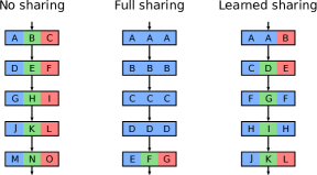
Figure 1: Different weight sharing schemes to solve a three-task MTL problem. Each box depicts a network layer and the letters denote different weights. Colored partitions in each box illustrate which tasks share weights for that layer. Weights are never shared in the last layer because it is the task-specific output layer. No sharing: When disregarding the possibility to perform MTL, an independent set of weights is used in every task-specific network. Full sharing: Sometimes called shared back-bone in literature, this scheme shares weights in all but the final layer. Learned sharing: A weight assignment learned by our method on the DKL-MNIST dataset.

The difficulty then lies in choosing an appropriate weight sharing configuration from this extremely large search space. We introduce an automatic method that learns how to share layer weights between task-specific networks using alternating optimization with a natural evolution strategy (NES) and stochastic gradient descent (SGD). The main problem is the non-differentiable assignment between weights and layers that prevents learning both the assignment and weights with SGD. Therefore, we exploit the black-box nature of NES to optimize a probability distribution over the non-differentiable assignment. It would also be possible to learn the weights themselves with NES but this is rather inefficient compared to SGD. Since for every fixed assignment the networks become differentiable wrt. their weights, we exploit SGD to efficiently train them.

While alternating these two steps, the probability distribution’s entropy decreases and the layer weights are optimized to perform well under the most likely assignments. In the end, this results in a single most likely assignment and corresponding layer weights. Notably, this is achieved without resorting to costly fitness evaluation steps that have to train networks from scratch, or differentiable weight sharing approaches [5, 6, 7] that result in computationally intensive forward passes during inference.

Using our learned weight sharing (LWS) method, we show accuracy improvements compared to our own baselines and baselines from literature on three datasets.

II Related Work

The general approach that powers LWS is a hybrid optimization of differentiable and non-differentiable parameters. Such a concept is used in [8] to perform neural architecture search. The non-differentiable parameters govern what kinds of layers are used in the architecture and are optimized in an alternating fashion together with the layer weights. Similarly, in [9] the non-differentiable parameters are sparsity masks inside a network and the differentiable parameters are again layer weights. This allows to train sparse networks directly instead of sparsifying them after first training a dense model.

Next, we will present deep MTL literature to position our work against existing methods and then NES literature to provide background for understanding the method.

II-A Deep Multi-Task Learning

The main difference between various deep multi-task learning approaches is how weight sharing between tasks is implemented. This decision is encoded in the architecture of a deep neural network, either by the designer or an algorithm. Early works usually employ a shared neural network that branches into small task-specific parts at its end [10, 11]. This approach, referred to as full sharing in this paper, is restrictive because all tasks have to work on exactly the same representation, even if the tasks are very different. This motivated further work to lift this restriction and make weight sharing data-dependent.

Approaches like cross-stitch networks [5], Sluice networks [6] or soft layer ordering [7] introduce additional parameters that control the weight sharing and are jointly optimized with the networks weights by SGD. In these approaches, the task-specific networks are connected by gates between every layer that perform weighted sums between the individual layer’s outputs. The coefficients of these weighted sums are learned and can therefore control the influence that different tasks have on each other. However, since all task-specific networks are interconnected, this approach requires to evaluate all of them even when performing inference on only a single task. In contrast, every task-specific network in LWS can be used for inference independently. Soft layer ordering further has the restriction that all shareable layers at any position in the network must be compatible in input and output shape. LWS on the other hand is unrestricted by the underlying network architecture and can for example be applied to residual networks.

Another set of works explores non-differentiable ways to share weights. Examples include fully-adaptive feature sharing, which iteratively builds a branching architecture that groups similar tasks together [12] or routing networks, which use reinforcement learning to choose a sequence of modules from a shared set of modules in a task-specific way [13]. Routing networks are similar to our work in that they also avoid the interconnection between task-specific networks as described before. However, their approach fundamentally differs in that their routing network chooses layers in a data-dependent way on a per-example basis, while our network configuration is fixed after training and only differs between tasks not examples.

II-B Natural Evolution Strategy

Natural Evolution Strategy refers to a class of black-box optimization algorithms that update a search distribution in the direction of higher expected fitness using the natural gradient [14]. Given a parameterized search distribution with probability density function $q\left(\left.x\right|\alpha\right)$, and a fitness function $u\left(x\right)$, the expected fitness is

$$J\left(\alpha\right)=\mathbb{E}_{q_{\alpha}}\left[u\left(x\right)\right].$$ (1)

The plain gradient in the direction of higher expected fitness can be approximated from samples $x_{1},\ldots,x_{\lambda}$ distributed according to $q\left(\left.x\right|\alpha\right)$ by a Monte-Carlo estimate as

$$\nabla_{\alpha}J\left(\alpha\right)\approx\frac{1}{\lambda}\sum_{i=1}^{\lambda}u\left(x_{i}\right)\nabla_{\alpha}\log q\left(\left.x_{i}\right|\alpha\right)$$ (2)

with population size $\lambda$. Instead of following the plain gradient directly, NES follows the natural gradient $\mathbf{F}^{-1}\nabla_{\alpha}J\left(\alpha\right)$. Here, $\mathbf{F}^{-1}$ refers to the inverse of the search distribution’s Fisher information matrix. The natural gradient offers, among others, increased convergence speed on flat parts of the fitness landscape.

The Fisher information matrix depends only on the probability distribution itself and can often be analytically derived, e.g. for the common case of multinormal search distributions [15]. For the case of search distributions from the exponential family under expectation parameters, a direct derivation of the natural gradient without first calculating $\mathbf{F}$ exists [16, page 57]. The probability density function for members of the exponential family has the form

$$q\left(\left.x\right|\alpha\right)=h\left(x\right)\exp\left\{\alpha\cdot T\left(x\right)-A\left(\alpha\right)\right\}$$ (3)

with natural parameter vector $\alpha$, sufficient statistic vector $T\left(x\right)$ and cumulant function $A\left(\alpha\right).$ We focus only on the case where $h\left(x\right)=1$ in our paper. If we reparameterize the distribution with a parameter vector $\mu$ that satisfies

$$\mu=\mathbb{E}_{q_{\alpha}}\left[T\left(x\right)\right]=\nabla_{\alpha}A\left(\alpha\right),$$ (4)

then we call $\mu$ the expectation parameters. With such a parameterization, there is a nice result regarding the natural gradient: The natural gradient wrt. the expectation parameters is given by the plain gradient wrt. the natural parameters, i.e.

$$\tilde{\nabla}_{\mu}q\left(\left.x\right|\mu\right)=\nabla_{\alpha}q\left(\left.x\right|\alpha\right).$$ (5)

It follows that the log-derivative, which is necessary for the search gradient estimate in NES, can easily be derived as

$$\tilde{\nabla}_{\mu}\log q\left(\left.x\right|\mu\right) =\nabla_{\alpha}\log q\left(\left.x\right|\alpha\right)$$ (6)

$$=\nabla_{\alpha}\left(\alpha\cdot T\left(x\right)-A\left(\alpha\right)\right)$$ (7)

$$=T\left(x\right)-\mu$$ (8)

because of the relationship in Equation 4 between gradient of the cumulant function and expectation parameters.

In other words, if we choose a search distribution with expectation parameters, the plain and natural gradient coincide. We will use this fact later, to follow the natural gradient of a categorical distribution.

III Learned Weight Sharing

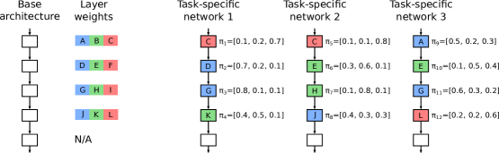
Figure 2: Setup to solve a three-task MTL problem with LWS. A base architecture is duplicated for each task and weights are stochastically assigned to each layer. There are a total of $N=12$ layers and $K=3$ weights per weight set. The depicted assignment is the most probable one, which is used for inference.

Consider the setup depicted in Figure 2 to solve an MTL problem using deep neural networks. Any neural network architecture is chosen as the base architecture, e.g. a residual network. This base architecture is duplicated once for each task to create task-specific networks. Finally, the last layer of each task-specific network is modified to have the appropriate number of outputs for the task.

In this setup, the weights of every layer except for the last one are compatible between task-specific networks and can potentially be shared. To this end, a set of $K$ weights is created for every layer and all of the $N$ task-specific network layers are assigned a weight from its corresponding set. By assigning the same weight to multiple task-specific networks, weight sharing is achieved. The number of weights per layer must not necessarily be the same, however we restrict ourselves to equally sized sets of weights for simplicity.

The problem is now to find good assignments between the weights and task-specific network layers and at at the same time train the weights themselves. We achieve this by alternating between the optimization of a search distribution over assignments with NES and the optimization of layer weights with SGD. This approach is summarized in Algorithm 1 and explained in more detail below.

1 Let $p\left(\left.a\right|\pi\right)$ be the search distribution over assignments

2 Let $f_{x,y}\left(\theta,a\right)$ be the loss for a batch of data $x,y$ under weights $\theta$ and assignment $a$

3 def $\mathtt{StepNES}$ $\left(\theta,\pi\right)$ as

4       $x,y\leftarrow$ get random batch

5       for $i$ in $1\ldots\lambda_{\pi}$ do

6             sample $a_{i}$ distributed according to $p\left(\left.a\right|\pi\right)$

7             calc. loss $l_{i}=f_{x,y}\left(\theta,a_{i}\right)$

8             calc. log-derivative $\nabla_{\pi}\log p\left(\left.a_{i}\right|\pi\right)$

9            

10       end for

11      calc. utilities $u_{i}=2\cdot\frac{\textrm{rank}\left(l_{i}\right)-1}{\lambda_{\pi}-1}-1$

12       $\nabla_{\pi}J_{\pi}=\frac{1}{\lambda_{\pi}}\sum_{i=1}^{\lambda_{\pi}}u_{i}\nabla_{\pi}\log p\left(\left.a_{i}\right|\pi\right)$

13       return $\pi+\eta_{\pi}\nabla_{\pi}J_{\pi}$

14      

15 end

16 def $\mathtt{StepSGD}$ $\left(\theta,\pi\right)$ as

17       $x,y\leftarrow$ get random batch

18       for $i$ in $1\ldots\lambda_{\theta}$ do

19             sample $a_{i}$ distributed according to $p\left(\left.a\right|\pi\right)$

20             calc. weight gradient $\nabla_{\theta}f_{x,y}\left(\theta,a_{i}\right)$

21            

22       end for

23      $\nabla_{\theta}J_{\theta}=\frac{1}{\lambda_{\theta}}\sum_{i=1}^{\lambda_{\theta}}\nabla_{\theta}f_{x,y}\left(\theta,a_{i}\right)$

24       return $\theta-\eta_{\theta}\nabla_{\theta}J_{\theta}$

25      

26 end

27 $\pi\leftarrow$ search distribution parameter vector with all $N\left(K-1\right)$ elements set to $\frac{1}{K}$

28 $\theta\leftarrow$ randomly initialized neural network weights

29 while not finished do

30       $\pi\leftarrow$ $\mathtt{StepNES}$ $\left(\theta,\pi\right)$

31       $\theta\leftarrow$ $\mathtt{StepSGD}$ $\left(\theta,\pi\right)$

32      

33 end while

Algorithm 1 LWS training procedure.

III-A Learning Objective

The search for good assignments and layer weights is cast as an optimization problem

$$\min_{\theta,a}f\left(\theta,a\right),$$ (9)

where $f:\Theta\times\mathcal{A}\rightarrow\mathbb{R}$ is the average loss over all tasks, $\theta\in\Theta$ is a vector of all layer weights, and $a\in\mathcal{A}$ is an assignment of weights to task-specific network layers. The loss function $f$ is differentiable wrt. $\theta$ but black-box wrt. $a$. We would like to exploit the fact that $\theta$ can be efficiently optimized by SGD but need a way to simultaneously optimize $a$. Therefore, we create a stochastic version of the problem

$$\min_{\theta,\pi}J\left(\theta,\pi\right)=\mathbb{E}_{p_{\pi}}\left[f\left(\theta,a\right)\right]$$ (10)

by introducing a probability distribution defined on $\mathcal{A}$ with density function $p\left(\left.a\right|\pi\right)$. This stochastic formulation makes the assignments amenable for optimization through $\pi$ by the NES algorithm, but on the other hand requires to sample assignments for the calculation of the gradient wrt. $\theta$.

III-B Assignment Optimization

We use the NES algorithm to optimize $\pi$ for lower expected loss $J\left(\theta,\pi\right)$ while keeping $\theta$ fixed (cf. Algorithm 1, lines 1 to 1). The parameter $\pi$ is initialized so that all assignments are equally probable but with prior knowledge the initial parameter vector could also be chosen so that it is biased towards certain preferred assignments.

Assignments $a_{1},\ldots,a_{\lambda_{\pi}}$ distributed according to $p\left(\left.a\right|\pi\right)$ are sampled and their loss values $l_{i}=f\left(\theta,a_{i}\right)$ are calculated on the same batch of training data for all assignments. Following Equation 2, the search gradient is approximated as

$$\nabla_{\pi}J\left(\theta,\pi\right)\approx\frac{1}{\lambda_{\pi}}\sum_{i=1}^{\lambda_{\pi}}u_{i}\nabla_{\pi}\log p\left(\left.a_{i}\right|\pi\right)$$ (11)

with utility values $u_{i}$ in place of fitness values (see below). Finally, $\pi$ is updated by performing a step in the direction of $\nabla_{\pi}J\left(\theta,\pi\right)$ scaled by a learning rate parameter $\eta_{\pi}$. This is basic SGD but in principle more sophisticated optimizers like SGD with momentum or Adam could be used for this update step as well.

The utility values are created by fitness shaping to make the algorithm invariant to the scale of the loss function. Loss values $l_{i}$ are transformed into utility values

$$u_{i}=2\cdot\frac{\textrm{rank}\left(l_{i}\right)-1}{\lambda_{\pi}-1}-1,$$ (12)

where $\textrm{rank}\left(l_{i}\right)$ ranks the loss values from 1 to $\lambda_{\pi}$ in descending order, i.e. the smallest $l_{i}$ receives rank $\lambda_{\pi}$. This results in equally spaced utility values in $\left[-1,1\right]$ with the lowest loss value receiving a utility value of 1.

III-C Layer Weight Optimization

While we can use backpropagation to efficiently determine the weight gradient $\nabla_{\theta}f\left(\theta,a\right)$ with $a$ fixed, determining $\nabla_{\theta}J\left(\theta,\pi\right)$ with $\pi$ fixed on the stochastic problem version is not possible directly. Instead, we use a Monte-Carlo approximation to optimize $\theta$ for lower expected loss $J\left(\theta,\pi\right)$ while keeping $\pi$ fixed (cf. Algorithm 1, lines 1 to 1).

In the beginning, all layer weights $\theta$ are randomly initialized. For the Monte-Carlo gradient estimation, assignments $a_{1},\ldots,a_{\lambda_{\theta}}$ distributed according to $p\left(\left.a\right|\pi\right)$ are sampled and backpropagation is performed for each sample. The same batch of training data is used for the backpropagation step throughout this process for every assignment. The resulting gradients $\nabla_{\theta}f\left(\theta,a_{i}\right)$ are averaged over all assignments, so that the final gradient is given by

$$\nabla_{\theta}J\left(\theta,\pi\right)\approx\frac{1}{\lambda_{\theta}}\sum_{i=1}^{\lambda_{\theta}}\nabla_{\theta}f\left(\theta,a_{i}\right).$$ (13)

Using this gradient, $\theta$ is updated by SGD with learning rate $\eta_{\theta}$ but, again, more sophisticated optimizers could be employed instead.

III-D Natural Gradient

The NES search gradient calculation in Equation 11 actually follows the plain gradient instead of the natural gradient unless we take care to use a specific parameterization for the search distribution. As previously explained, the natural gradient and plain gradient coincide when the distribution is a member of the exponential family and has expectation parameters. In our problem setting, there are a total of $N$ layers distributed over all task-specific networks that need to be assigned a weight from $K$ possible choices from the weight set corresponding to each layer. We can model this with categorical distributions, which are part of the exponential family, as follows.

First, consider a categorical distribution over $K$ categories with samples $x\in\mathbb{N}_{K}$. It is well known [17], that the categorical distribution can be written in exponential family form (cf. Equation 3) with natural parameters $\alpha\in\mathbb{R}^{K-1}$ as

$$p_{\textrm{nat}}\left(\left.x\right|\alpha\right) =\exp\bigl{\{}\alpha\cdot T_{\textrm{nat}}\left(x\right)-A_{\textrm{nat}}\left(\alpha\right)\bigr{\}}$$ (14)

$$T_{\textrm{nat}}\left(x\right) =\begin{pmatrix}\delta_{1,x}&\cdots&\delta_{K-1,x}\end{pmatrix}$$ (15)

$$A_{\textrm{nat}}\left(\alpha\right) =\log\left(1+\sum_{i=1}^{K-1}e^{\alpha_{i}}\right),$$ (16)

where $\delta_{i,j}$ is the Kronecker delta function that is 1 if $i=j$ and 0 otherwise. Our goal is to have this distribution in expectation parameters so that we can use the results mentioned before for the natural gradient calculation. We can reparameterize the distribution as

$$p_{\textrm{ex}}\left(\left.x\right|\mu\right) =\exp\bigl{\{}r_{\textrm{ex}}\left(\mu\right)\cdot T_{\textrm{ex}}\left(x\right)-A_{\textrm{ex}}\left(\mu\right)\bigr{\}}$$ (17)

$$r_{\textrm{ex}}\left(\mu\right) =\begin{pmatrix}\log\frac{\mu_{1}}{\mu_{K}}&\cdots&\log\frac{\mu_{K-1}}{\mu_{K}}\end{pmatrix}$$ (18)

$$T_{\textrm{ex}}\left(x\right) =\begin{pmatrix}\delta_{1,x}&\cdots&\delta_{K-1,x}\end{pmatrix}$$ (19)

$$A_{\textrm{ex}}\left(\mu\right) =-\log\mu_{K},$$ (20)

which gives us a parameter vector $\mu\in\left[0,1\right]^{K-1}$ with entries corresponding to the probabilities of all but the last category. For notational convenience, we use $\mu_{K}=1-\sum_{i=1}^{K-1}\mu_{i}$ even though it is not technically part of the parameter vector.

To see that $\mu$ are expectation parameters, we compare it to the derivative of the cumulant function in natural parameters (cf. Equation 4). By using the relationship $\alpha_{i}=\log\frac{\mu_{i}}{\mu_{K}}$ it is easy to show that

$$\frac{\partial A_{\textrm{nat}}\left(\alpha\right)}{\partial\alpha_{i}} =\frac{e^{\alpha_{i}}}{1+\sum_{j=1}^{K-1}e^{\alpha_{j}}}=\mu_{i}$$ (21)

holds for all $i\in\mathbb{N}_{K-1}$.

Now, consider a joint of $N$ independent but not identically distributed categorical distributions with samples $a$ and parameters $\pi$ so that

$$a =\begin{pmatrix}a_{1}&\cdots&a_{N}\end{pmatrix}\in\mathbb{N}_{K}^{N}$$ (22)

$$\pi =\begin{pmatrix}\pi_{1}&\cdots&\pi_{N}\end{pmatrix}\in\left[0,1\right]^{N\left(K-1\right)}$$ (23)

are the concatenations of the samples and expectation parameters of all $N$ categorical distributions, i.e. $\pi$ is the concatenation of $N$ expectation parameter vectors $\pi_{i}\in\left[0,1\right]^{K-1}$.

Due to the independence of the $N$ categorical distributions, the density function for the joint distribution becomes the product of their individual densities. Again, this is a member of the exponential family with expectation parameters:

$$p\left(\left.a\right|\pi\right) ={\textstyle\prod\nolimits}_{i=1}^{N}p_{\textrm{ex}}\left(\left.a_{i}\right|\pi_{i}\right)$$ (24)

$$=\exp\bigl{\{}r\left(\pi\right)\cdot T\left(a\right)-A\left(\pi\right)\bigr{\}}$$ (25)

$$r\left(\pi\right) =\begin{pmatrix}r_{\textrm{ex}}\left(\pi_{1}\right)&\cdots&r_{\textrm{ex}}\left(\pi_{N}\right)\end{pmatrix}$$ (26)

$$T\left(a\right) =\begin{pmatrix}T_{\textrm{ex}}\left(a_{1}\right)&\cdots&T_{\textrm{ex}}\left(a_{N}\right)\end{pmatrix}$$ (27)

$$A\left(\pi\right) ={\textstyle\sum\nolimits}_{i=1}^{N}A_{\textrm{ex}}\left(\pi_{i}\right).$$ (28)

In summary, LWS uses $p\left(\left.a\right|\pi\right)$ from Equation 24 as the density for its search distribution. The parameters $\pi$ are the concatenation of all but the last probabilities for each categorical distribution. Since $\pi$ are expectation parameters, we can use Equation 8 to calculate the natural gradient as

$$\nabla_{\pi}\log p\left(\left.a\right|\pi\right)=T\left(a\right)-\pi$$ (29)

and plug it into Algorithm 1 at line 1.

III-E Inference

After training has finished, the most likely weight assignment $\arg\max_{a}p\left(\left.a\right|\pi\right)$ is used for inference.

IV Experiments

Table I: Test error of learned weight sharing compared to full sharing and no sharing baselines.

	DLK-MNIST	CIFAR-100	Omniglot
Method	ConvNet	ResNet18	ResNet18
Full sharing	14.16 $\pm$ 0.37	31.80 $\pm$ 0.44	10.97 $\pm$ 0.60
No sharing	12.80 $\pm$ 0.16	32.53 $\pm$ 0.32	15.82 $\pm$ 1.02
Learned sharing	11.83 $\pm$ 0.51	30.84 $\pm$ 0.49	10.70 $\pm$ 0.62

We demonstrate the performance of LWS on three different multi-task datasets using convolutional network architectures taken from other MTL publications to compare our results to theirs. We also perform experiments using a residual network [18] architecture to show applicability of LWS to modern architectures. Furthermore, we provide two baseline results for all experiments which are full sharing, i.e. every task shares weights with every other task at each layer except for the last one, and no sharing, i.e. all task-specific networks are completely independent. Note that a completely independent network for each task means that its whole capacity is available to learn a single task, whereas the full sharing network has to learn all tasks using the same capacity. Depending on network capacity, task difficulty and task compatibility we will see no sharing outperform full sharing and also the other way around.

All experiments are repeated 10 times and reported with mean and standard deviation. For statistical significance tests, we perform a one-sided Mann-Whitney U test. The search distribution parameters $\pi$ are initialized to $\frac{1}{K}$ so that layers are chosen uniformly at random in the beginning. Furthermore, to prevent that a layer will never be chosen again once its probability reaches zero, every entry in $\pi$ is clamped above 0.1 % after the update step and then $\pi$ is renormalized to sum to one. The layer weights $\theta$ are initialized with uniform He initialization [19] and update steps on $\theta$ are performed with the Adam [20] optimizer. All images used in the experiments are normalized to $\left[0,1\right]$ and batches are created by sampling 16 training examples from each different task and concatenating them. Full sharing, no sharing, and LWS all use the same equal loss weighting between different tasks. MTL is usually sensitive to this weighting and further improvements might be achieved but its optimization is left for future work. All source code is publicly available online.

IV-A DKL-MNIST

DKL-MNIST is a custom MTL dataset created from the Extended-MNIST [21] and Kuzushiji-MNIST [22] image classification datasets. We select 500 training examples of digits, letters and kuzushiji each for a total of 1,500 training examples and keep the complete test sets for a total of 70,800 test examples. Using only a few training examples per task creates a situation where sharing features between tasks should improve performance. Since all three underlying datasets are MNIST variants, the training examples are $28\times 28$ grayscale images but there are 10 digit classes, 26 letter classes and 10 kuzushiji classes in each task respectively.

For this small dataset, we use a custom convolutional network architecture that consists of three convolutional layers and two dense layers. The convolutions all have 32 filters, kernel size $3\times 3$ and are followed by batch normalization, ReLU activation and $2\times 2$ max-pooling. The first dense layer has 128 units and is followed by a ReLU activation, while the second dense layer has as many units as there are classes for the task. LWS is applied to the three convolutional layers and the first dense layer, i.e. the whole network except for the task-specific last layer.

We train LWS and the two baselines for 5,000 iterations on DKL-MNIST using a SGD learning rate of $\eta_{\theta}=10^{-3}$. Furthermore, LWS uses $\lambda_{\theta}=\lambda_{\pi}=8$ samples for both SGD and NES, and a NES learning rate of $\eta_{\pi}=10^{-2}$ to learn to share sets of $K=3$ weights for each layer. We see in Table I that full sharing performs worse than no sharing, i.e. there is negative transfer when using the simple approach of sharing all but the last layer. However, using LWS we find an assignment that is significantly ($p<0.01$) better than the no sharing baseline for a total error of 11.83 %.

IV-B CIFAR-100

Table II: Comparison against results from [13] using their network architecture.

Method	CIFAR-100 Test Error [%]
Cross-stitch networks [13]	47
Routing networks [13]	40
Full sharing	39.08 $\pm$ 0.36
No sharing	36.50 $\pm$ 0.43
Learned sharing	37.43 $\pm$ 0.53

The CIFAR-100 image classification dataset is cast as an MTL problem by grouping the different classes into tasks by the 20 coarse labels that CIFAR-100 provides. Each task then contains 5 classes and 2,500 training examples (500 per class) for a total of 50,000 training examples and 10,000 test examples, all of which are $32\times 32$ pixel RGB images.

We employ the neural network architecture given by [13] to allow for a comparison against their results. It consists of four convolutional layers and four dense layers. The convolutions all have 32 filters and kernel size $3\times 3$, and are followed by batch normalization, ReLU activation and $2\times 2$ max-pooling. The first three dense layers all have 128 units and are followed by a ReLU activation, while the last dense layer has as many units as there are classes for the task, i.e. 5 for all tasks on this dataset. In [13] they only apply their MTL method to the three dense layers with 128 units so we do the same for a fair comparison. This means the convolutional layers always share their weights between all tasks.

We train LWS and the two baselines for 4,000 iterations on CIFAR-100 using a SGD learning rate of $\eta_{\theta}=10^{-3}$. Furthermore, LWS uses $\lambda_{\theta}=\lambda_{\pi}=8$ samples for SGD and NES, and a NES learning rate of $\eta_{\pi}=10^{-1}$ to learn to share sets of $K=20$ weights for each layer. Table II shows that LWS, with a test error of 37.43 %, outperforms both cross-stitch networks at 47 % test error and routing networks at 40 % test error. However, no sharing achieves even better results. This can be attributed to the network capacity being small in relation to the dataset difficulty. In this case, having 20 times more weights is more important than sharing data between tasks.

Therefore, we repeat the experiment with a ResNet18 architecture that has much higher capacity than the custom convolutional network from [13]. The channel configuration in our ResNet18 is the same as in the original publication [18]. However, due to the much smaller image size of CIFAR-100, we remove the $3\times 3$ max-pooling layer and set the convolutional stride parameters so that downsampling is only performed in the last three stages. We apply LWS to share weights between each residual block. They are treated as a single unit that consists of two convolutional layers and, in the case of a downsampling block, a third convolutional layer in the shortcut connection. All hyperparameters stay the same except for the amount of iterations, which is increased to 20,000. Test curves are shown in Figure 5 and final test results are listed in Table I. We notice that no sharing at 32.53 % test error now performs worse than full sharing at 31.80 % test error. We believe the reason to be the increased network capacity that is now high enough to benefit from data sharing between tasks. LWS further improves on this and achieves the lowest test error at 30.84 %, which is significantly ($p<0.01$) better than full sharing.

Depending on the sharing configuration, the total number of weights that are present in the system comprised of all task-specific networks differs. Naturally, the no sharing configuration has the highest possible amount of weights at 223M, while full sharing has the lowest possible amount at 11M. They differ exactly by a factor of 20, which is the number of tasks in this setting. LWS finds a configuration that uses 136M weights while still achieving higher accuracy than both baselines.

IV-C Omniglot

Table III: Comparison against results from [7] using their network architecture.

Method	Omniglot Test Error [%]
Soft layer ordering [7]	24.1
Full sharing	20.85 $\pm$ 1.07
No sharing	23.52 $\pm$ 1.25
Learned sharing	19.31 $\pm$ 2.54

The Omniglot dataset [23] is a standard MTL dataset that consists of handwritten characters from 50 different alphabets, each of which poses a character classification task. The alphabets contain varying numbers of characters, i.e. classes, with 20 grayscale example images of $105\times 105$ pixels each. Since Omniglot contains no predefined train-test-split, we randomly split off 20 % as test examples from each alphabet.

We employ the neural network architecture given by [7] to allow for a comparison against their results. It consists of four convolutional layers and a single dense layer. The convolutional layers all have 53 filters and kernel size $3\times 3$ and are followed by batch normalization, ReLU activation and $2\times 2$ max-pooling. The final dense layer has as many units as there are classes for the task. As in [7], we apply LWS to the four convolutional layers.

We train LWS and the two baselines for 20,000 iterations on Omniglot using a SGD learning rate of $\eta_{\theta}=10^{-3}$. Furthermore, LWS uses $\lambda_{\theta}=\lambda_{\pi}=8$ samples for SGD and NES, and a NES learning rate of $\eta_{\pi}=10^{-2}$ to learn to share sets of $K=20$ weights for each layer. Table III shows how LWS outperforms SLO and both baselines. We repeat the experiment with a ResNet18 architecture with the $3\times 3$ max-pooling removed and present results in Table I. LWS still performs significantly ($p<0.01$) better than no sharing and is on par with full sharing. Neither full sharing nor LWS is significantly ($p<0.01$) better than the other.

IV-D Qualitative Results

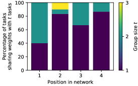
Figure 3: Percentage of tasks that share weights between exactly $t$ tasks when learned with LWS on DKL-MNIST.

Figure 3 sheds light on what kind of assignments are learned on the DKL-MNIST dataset. The three convolutional layers and the one dense layers that are shareable are denoted on the horizontal axis in the same order as in the network itself. For each layer, a stacked bar represents the percentage of tasks over all repetitions that shared the layer weight within a group of $t$ tasks. Since there are three tasks and three weights per shared set the only possible assignments are (1) all three tasks have independent weights, (2) two tasks share the same weight, while the last task has an independent weight, and (3) all three tasks share the same weight. In Figure 3 the group sizes correspond to these three assignments, e.g. in 40 % of the experiments the first layer had three tasks with independent weights. An exemplary assignment that was found in one of the DKL-MNIST experiments can be seen in Figure 1.

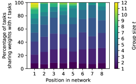
Figure 4: Percentage of tasks that share weights between exactly $t$ tasks when learned with LWS on Omniglot.

Figure 4 shows the same kind of visualization on Omniglot for a ResNet18. Due to the vastly increased number of possible assignments, the interpretation is not as straightforward as in the DKL-MNIST case. However, we can clearly see how weights are shared between a larger number of tasks in the early layers. This corresponds well to results from transfer learning literature [24], where early convolutional layers have been found to learn very general filters.

V Conclusion

LWS solves MTL problems by learning how to share weights between task-specific networks. We show how combining NES and SGD creates a learning algorithm that deals with the problem’s non-differentiable structure by NES, while still exploiting the parts that are differentiable with SGD. This approach beats the MTL approaches cross-stitch networks, routing networks and soft layer ordering on their respective problems and we show good performance on three datasets using a large-scale residual network.

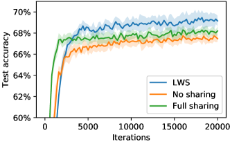
Figure 5: Test accuracy during training for LWS and its baselines using a ResNet18 on CIFAR-100.

References

- [1] S. Lee, C. Lee, D. Kwak, J. Kim, J. Kim, and B. Zhang, “Dual-memory deep learning architectures for lifelong learning of everyday human behaviors,” in Proceedings of the Twenty-Fifth International Joint Conference on Artificial Intelligence, IJCAI 2016, New York, NY, USA, 9-15 July 2016, 2016, pp. 1669–1675. [Online]. Available: http://www.ijcai.org/Abstract/16/239
- [2] C. Fernando, D. Banarse, C. Blundell, Y. Zwols, D. Ha, A. A. Rusu, A. Pritzel, and D. Wierstra, “Pathnet: Evolution channels gradient descent in super neural networks,” CoRR, vol. abs/1701.08734, 2017. [Online]. Available: http://arxiv.org/abs/1701.08734
- [3] C. Tessler, S. Givony, T. Zahavy, D. J. Mankowitz, and S. Mannor, “A deep hierarchical approach to lifelong learning in minecraft,” in Proceedings of the Thirty-First AAAI Conference on Artificial Intelligence, February 4-9, 2017, San Francisco, California, USA., 2017, pp. 1553–1561. [Online]. Available: http://aaai.org/ocs/index.php/AAAI/AAAI17/paper/view/14630
- [4] R. Caruana, “Multitask learning,” Machine Learning, vol. 28, no. 1, pp. 41–75, Jul 1997. [Online]. Available: https://doi.org/10.1023/A:1007379606734
- [5] I. Misra, A. Shrivastava, A. Gupta, and M. Hebert, “Cross-stitch networks for multi-task learning,” in 2016 IEEE Conference on Computer Vision and Pattern Recognition, CVPR 2016, Las Vegas, NV, USA, June 27-30, 2016, 2016, pp. 3994–4003. [Online]. Available: https://doi.org/10.1109/CVPR.2016.433
- [6] S. Ruder, J. Bingel, I. Augenstein, and A. Søgaard, “Sluice networks: Learning what to share between loosely related tasks,” CoRR, vol. abs/1705.08142, 2017. [Online]. Available: http://arxiv.org/abs/1705.08142
- [7] E. Meyerson and R. Miikkulainen, “Beyond shared hierarchies: Deep multitask learning through soft layer ordering,” in 6th International Conference on Learning Representations, ICLR 2018, Vancouver, BC, Canada, April 30 - May 3, 2018, Conference Track Proceedings, 2018. [Online]. Available: https://openreview.net/forum?id=BkXmYfbAZ
- [8] Y. Akimoto, S. Shirakawa, N. Yoshinari, K. Uchida, S. Saito, and K. Nishida, “Adaptive stochastic natural gradient method for one-shot neural architecture search,” in Proceedings of the 36th International Conference on Machine Learning, ICML 2019, 9-15 June 2019, Long Beach, California, USA, 2019, pp. 171–180. [Online]. Available: http://proceedings.mlr.press/v97/akimoto19a.html
- [9] K. Lenc, E. Elsen, T. Schaul, and K. Simonyan, “Non-differentiable supervised learning with evolution strategies and hybrid methods,” CoRR, vol. abs/1906.03139, 2019. [Online]. Available: http://arxiv.org/abs/1906.03139
- [10] Z. Zhang, P. Luo, C. C. Loy, and X. Tang, “Facial landmark detection by deep multi-task learning,” in Computer Vision - ECCV 2014 - 13th European Conference, Zurich, Switzerland, September 6-12, 2014, Proceedings, Part VI, 2014, pp. 94–108. [Online]. Available: https://doi.org/10.1007/978-3-319-10599-4_7
- [11] X. Liu, J. Gao, X. He, L. Deng, K. Duh, and Y. Wang, “Representation learning using multi-task deep neural networks for semantic classification and information retrieval,” in NAACL HLT 2015, The 2015 Conference of the North American Chapter of the Association for Computational Linguistics: Human Language Technologies, Denver, Colorado, USA, May 31 - June 5, 2015, 2015, pp. 912–921. [Online]. Available: http://aclweb.org/anthology/N/N15/N15-1092.pdf
- [12] Y. Lu, A. Kumar, S. Zhai, Y. Cheng, T. Javidi, and R. S. Feris, “Fully-adaptive feature sharing in multi-task networks with applications in person attribute classification,” in 2017 IEEE Conference on Computer Vision and Pattern Recognition, CVPR 2017, Honolulu, HI, USA, July 21-26, 2017, 2017, pp. 1131–1140. [Online]. Available: https://doi.org/10.1109/CVPR.2017.126
- [13] C. Rosenbaum, T. Klinger, and M. Riemer, “Routing networks: Adaptive selection of non-linear functions for multi-task learning,” in 6th International Conference on Learning Representations, ICLR 2018, Vancouver, BC, Canada, April 30 - May 3, 2018, Conference Track Proceedings, 2018. [Online]. Available: https://openreview.net/forum?id=ry8dvM-R-
- [14] D. Wierstra, T. Schaul, T. Glasmachers, Y. Sun, J. Peters, and J. Schmidhuber, “Natural evolution strategies,” J. Mach. Learn. Res., vol. 15, no. 1, pp. 949–980, 2014. [Online]. Available: http://dl.acm.org/citation.cfm?id=2638566
- [15] Y. Sun, D. Wierstra, T. Schaul, and J. Schmidhuber, “Stochastic search using the natural gradient,” in Proceedings of the 26th Annual International Conference on Machine Learning, ICML 2009, Montreal, Quebec, Canada, June 14-18, 2009, 2009, pp. 1161–1168. [Online]. Available: https://doi.org/10.1145/1553374.1553522
- [16] Y. Ollivier, L. Arnold, A. Auger, and N. Hansen, “Information-geometric optimization algorithms: A unifying picture via invariance principles,” J. Mach. Learn. Res., vol. 18, pp. 18:1–18:65, 2017. [Online]. Available: http://jmlr.org/papers/v18/14-467.html
- [17] C. J. Geyer, “Stat 5421 lecture notes: Exponential families, part i,” Apr. 2016. [Online]. Available: http://www.stat.umn.edu/geyer/5421/notes/expfam.pdf
- [18] K. He, X. Zhang, S. Ren, and J. Sun, “Deep residual learning for image recognition,” in 2016 IEEE Conference on Computer Vision and Pattern Recognition, CVPR 2016, Las Vegas, NV, USA, June 27-30, 2016, 2016, pp. 770–778. [Online]. Available: https://doi.org/10.1109/CVPR.2016.90
- [19] ——, “Delving deep into rectifiers: Surpassing human-level performance on imagenet classification,” in 2015 IEEE International Conference on Computer Vision, ICCV 2015, Santiago, Chile, December 7-13, 2015, 2015, pp. 1026–1034. [Online]. Available: https://doi.org/10.1109/ICCV.2015.123
- [20] D. P. Kingma and J. Ba, “Adam: A method for stochastic optimization,” in 3rd International Conference on Learning Representations, ICLR 2015, San Diego, CA, USA, May 7-9, 2015, Conference Track Proceedings, 2015. [Online]. Available: http://arxiv.org/abs/1412.6980
- [21] G. Cohen, S. Afshar, J. Tapson, and A. van Schaik, “EMNIST: extending MNIST to handwritten letters,” in 2017 International Joint Conference on Neural Networks, IJCNN 2017, Anchorage, AK, USA, May 14-19, 2017, 2017, pp. 2921–2926. [Online]. Available: https://doi.org/10.1109/IJCNN.2017.7966217
- [22] T. Clanuwat, M. Bober-Irizar, A. Kitamoto, A. Lamb, K. Yamamoto, and D. Ha, “Deep learning for classical japanese literature,” CoRR, vol. abs/1812.01718, 2018. [Online]. Available: http://arxiv.org/abs/1812.01718
- [23] B. M. Lake, R. Salakhutdinov, and J. B. Tenenbaum, “Human-level concept learning through probabilistic program induction,” Science, vol. 350, no. 6266, pp. 1332–1338, 2015. [Online]. Available: https://science.sciencemag.org/content/350/6266/1332
- [24] J. Yosinski, J. Clune, Y. Bengio, and H. Lipson, “How transferable are features in deep neural networks?” in Advances in Neural Information Processing Systems 27: Annual Conference on Neural Information Processing Systems 2014, December 8-13 2014, Montreal, Quebec, Canada, 2014, pp. 3320–3328. [Online]. Available: http://papers.nips.cc/paper/5347-how-transferable-are-features-in-deep-neural-networks