Depth Edge Guided CNNs for Sparse Depth Upsampling

Abstract

Guided sparse depth upsampling aims to upsample an irregularly sampled sparse depth map when an aligned high-resolution color image is given as guidance. Many neural networks have been designed for this task. However, they often ignore the structural difference between the depth and the color image, resulting in obvious artifacts such as texture copy and depth blur at the upsampling depth. Inspired by the normalized convolution operation, we propose a guided convolutional layer to recover dense depth from sparse and irregular depth image with an depth edge image as guidance. Our novel guided network can prevent the depth value from crossing the depth edge to facilitate upsampling. We further design a convolution network based on proposed convolutional layer to combine the advantages of different algorithms and achieve better performance. We conduct comprehensive experiments to verify our method on real-world indoor and synthetic outdoor datasets. Our method produces strong results. It outperforms state-of-the-art methods on the Virtual KITTI dataset and the Middlebury dataset. It also presents strong generalization capability under different 3D point densities, various lighting and weather conditions.

Keywords Sparse Depth  $\cdot$ CNNs  $\cdot$ Depth Upsampling  $\cdot$ Normalized Convolution  $\cdot$ Depth Edge

1 Introduction

The purpose of sparse depth upsampling is to reconstruct dense depth maps from sparsely measured data that is not regularly sampled. Since the combination of 3D laser scanners and cameras became popular in autonomous driving, this task has received considerable attention. Due to the limitation of hardware development, the most advanced range sensors today still achieve much lower resolution data than visual images. Even for the Velodyne HDL-64e [1], when a sparse 3D point cloud is projected onto an aligned 2D image, it only obtains about 5% effective depth values in the projected image. Such a high sparsity level makes it challenging to perform subsequent tasks such as RGB-D based object detection[2, 3, 4, 5] and road scene understanding[6, 7].

While some methods[8, 9]operate directly on depth input for upsampling, others[10, 11, 12, 13, 14, 15, 16] require guidance, for example, from high-resolution images, and we’ll focus here. The basic assumption used to guide upsampling is that the target domain shares commonality with high-resolution guided images, for example, image edges are aligned with depth discontinuities. A popular choice for guided upsampling is guided bilateral filtering[17, 18, 19, 20, 21]. More advanced methods are based on global energy minimization[22, 12, 23, 13, 14], compressed sensing[24]or combined semantics to improve performance[25]. Some methods also use the end-to-end model to perform guided depth upsampling of regular data[15, 26].

Guided sparse depth upsampling methods are usually based on the assumption that depth edges consistently appear at the edges of the images. However, despite there are close connections between depth map and image, the discontinuities—especially the textures—of image are not always consistent with those of depth map. Using the color image as guidance, they ignore the structural difference between the depth and the guidance color image, resulting in obvious artifacts such as texture copy and depth blur at the upsampling depth.

We propose a novel sparse depth upsampling convolution layer(EGCL) using depth edge maps to better perform the sparse depth upsampling task. Different from previous methods, we transform the problem of sparse depth upsampling from color image guidance to depth edge guidance, because depth edges have special importance in non-textured depth images. Under the guidance of predicting the depth edge map, an improved confidence propagation CNNs[27] method is used to reconstruct the dense depth image. Depth edge guidance not only helps to avoid artifacts caused by direct image prediction, but also reduces aliasing artifacts and preserves sharp edges. Experiments on various datasets demonstrate that our approach outperforms the state-of-the-arts.

Based upon EGCL, we design a new architecture named edge guided convolutional neural network (EGCNN) to perform guided sparse depth upsampling. EGCNN consists of three major components: edge information extraction component, depth upsampling subnetwork, and depth fusion subnetwork. Edge information extraction component takes color images as input and outputs their edge-dist fields. Depth upsampling subnetwork applies EGCLs to deal with a sparse depth map with the guidance of edge-dist field. Depth fusion subnetwork is designed to fuse the outputs of depth upsampling subnetwork together to predict the dense upsampling result. Experiments show that this architecture can further improve performance.

2 Related Work

Since the emergence of active sensors with depth capabilities, depth completion has become a fundamental task in computer vision. In this section, we review previous literatures on this topic. Depending on whether there is an RGB image to guide the depth completion, previous methods can be roughly divided into two categories: non-guided methods and guided methods. We briefly review these techniques.

2.1 Non-guided Depth Upsampling

Methods for non-guided depth upsampling are closely related to those for single image super-resolution. Early methods were usually based on interpolation[28], sparse representation[29], and other traditional techniques. Recently, methods utilizing deep learning have achieved great success in both deep[8, 9]and color[30, 31]image super-resolution. Dahl et al.[32]presented a pixel recursive super resolution model that synthesizes realistic details into images while enhancing their resolution. Ma et al.[33] utilized an encoder-decoder architecture with self-supervised framework to predict the dense output. All of the above methods can handle regular low-resolution images but are not suitable for sparse data with irregular sampling.

To pay special attention to irregular sparse data, Chodosh et al.[34]used compressive sensing to handle sparsity, while using binary masks to filter out missing values. Uhrig et al.[9]proposed a sparse invariant convolution layer, which uses a binary effective mask to normalize sparse inputs. This layer is used to train a sparse depth mapping network with binary effective mask as input and dense depth mapping as output. Similarly, Hua and Gong[35]proposed a similar layer that uses a trained convolution filter to normalize sparse inputs. Instead, Jaritz et al.[36]compared different architectures and thought that using effective masks would degrade performance because masks in earlier layers in CNNs were saturated. However, this effect can be perfectly avoided by treating the binary validity masks as continuous confidence fields describing the reliability of the data proposed by Eldesokey et al.[27]. In addition, this supports confidence propagation, which helps track the reliability of data throughout the processing pipeline.

2.2 Guided Depth Upsampling

Due to the sub-optimal performance of unguided methods on the edges, some recent methods urge the use of guidance from auxiliary data, such as RGB images or surface normals. Traditional methods mainly rely on local filtering techniques such as joint bilateral filtering and global optimization techiniques such as Markov random fields. Tomasi et al.[10]proposed bilateral filtering which produces no phantom colors along edges in color images, and reduces phantom colors where they appear in the original image. Diebel et al.[12]exploited the fact that discontinuities in range and coloring tend to co-align to generate high-resolution, low-noise range images by integrating regular camera images into the range data. By relying on the assumption that pixels with similar colors are likely to belong to the same surface, Favaro et al.[37]proposed a novel scheme to recover depth maps containing thin structures based on nonlocal-means filtering regularization. Inspired by [37], the framework in [13]extended this regularization with an additional edge weighting scheme based on several image features based on the additional high-resolution RGB input in order to maintain fine detail and structure. These methods are able to deal with both regularly and irregularly sampled data, but they use hand-crafted features that limit their performance.

In recent years, researchers have come up with various deep learning methods. Ma et al.[33]adopted an early fusion scheme, combining sparse depth input with corresponding RGB images, and achieved good results. On the other hand, Jaritz et al.[36]argued that late fusion performed better on the architecture they proposed, which was also demonstrated in[35]. Wirges et al.[38]used a combination of RGB images and surface normals to guide the process of depth upsampling. Konno et al.[39]used residual interpolation to combine low-resolution depth maps with high-resolution RGB images to generate high-resolution depth maps. Based on[9], Huang et al.[40]utilized the sparsity-invariant layer to design a sparsity-invariant multi-scale encoder-decoder network for sparse depth completion with RGB guidance. Zhang et al.[41]proposed to predict surface normal and occlusion boundary from a deep network and further utilize them to help depth completion in indoor scenes. Qiu et al.[42] extended a similar surface normal as guidance idea to the outdoor environment and recovered dense depth from sparse LiDAR data.

The aforementioned approaches are usually based on the assumption that depth edges consistently appear at the edges of the RGB images. However, although there is a close connections between the depth map and the color image, the discontinuity (especially the texture) of the image is not always consistent with the depth map. Using the single color image as guidance, they ignore the structural difference between the depth and the guidance color image, and much irrelevant information such as textures on the color image will mislead upsampling task on the depth image. To address these problems, in this study, we implement depth edge map guided convolution as a layer in CNNs for sparse inputs inspired by [43] and [35]. Benefited from the guidance of depth edge information, our model gains better performance than other CNNs.

3 The Proposed Method

We propose a edge guided convolutional neural network (EGCNN) to perform sparse depth upsampling. Figure 1 illustrates the entire architecture. It consists of three major components: edge information extraction component, depth upsampling subnetwork, and depth fusion subnetwork.

The input to the pipeline is a very sparse projected LiDAR point cloud, an input confidence map which has zeros at missing pixels and ones otherwise, and a corresponding high-resolution RGB image. The color image is fed to an edge information extraction component to extract depth edge information. Afterwards, the continuous output depth edge map from the edge information extraction component, the sparse point cloud input and the input confidence are fed to a depth upsampling network, where we replace the standard convolutional layer by our modified edge guided convolutional layer. The outputs from the upsampling network are weighted and fed to a fusion network which produces the final dense depth map.

To explain our edge guided convolutional network, we first elaborate the design of the edge information extraction component in subsection 3.1. Then we introduce a novel convolution layer(EGCL) in subsection 3.2. In the next, we explain how EGCL can be used in a common convolution network, which is our depth upsampling network, in subsection 3.3. Finally, we elaborate architecture details about fusion network in subsection 3.4.

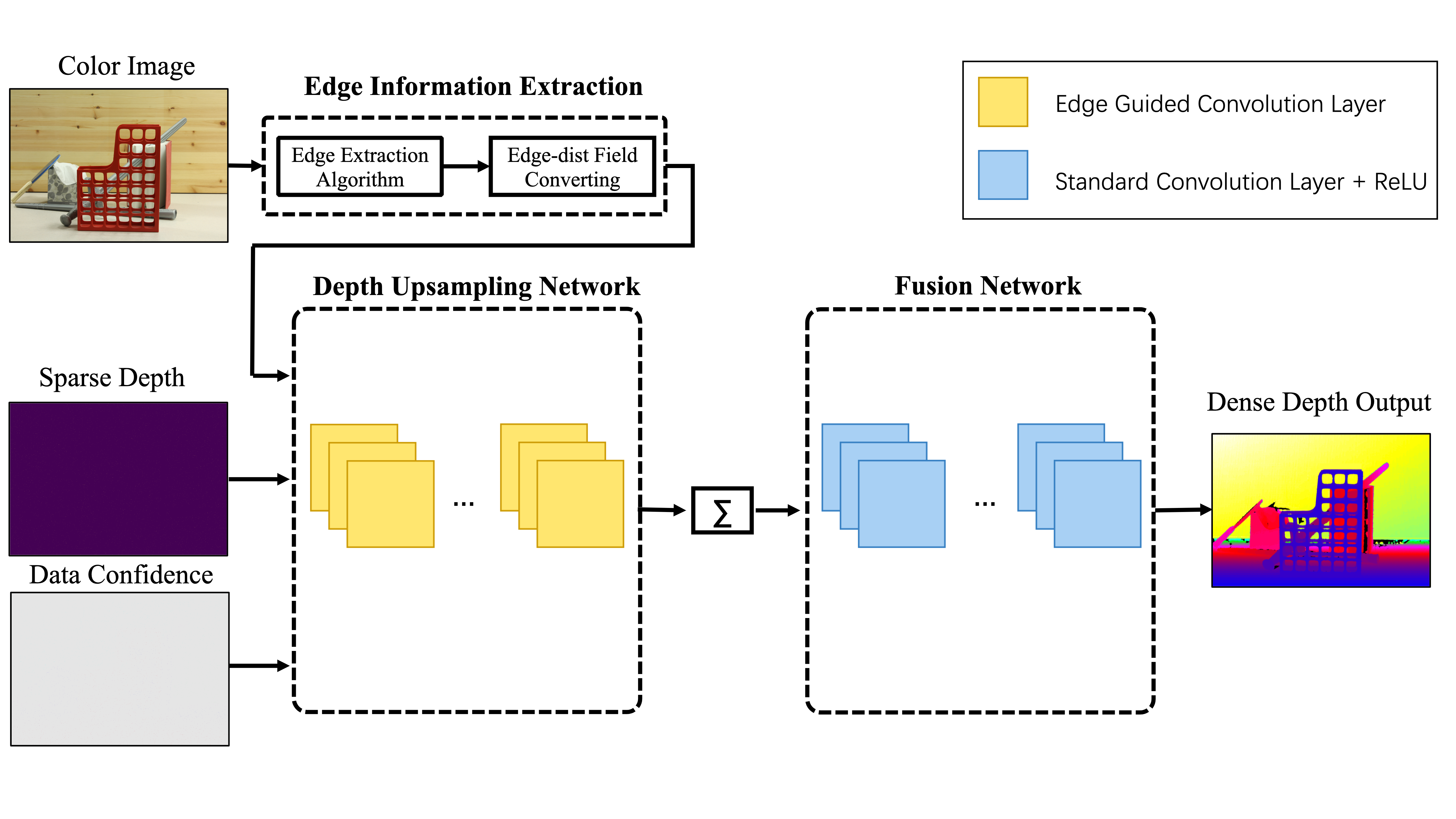
Figure 1: Our depth upsampling pipeline on an example image from the Middlebury dataset[44, 45].

3.1 Edge Information Extraction Component

As we observe, edges information is of especially importance in textureless depth map. Therefore, we design the edge information extraction component to obtain a continuous edge distance field from the color image, which guides the depth upsampling to generate sharp edges in the proposed method. As illustrated in Figure 2, the generation of edge-dist fields consists of two steps: 1) generating edge maps using edge extraction component from color images; 2) converting the edge map into our edge-dist field.

Edge extraction component is consist of multiple edge extraction nodes. Everyone of them takes color images $I$ as input and outputs different edge maps $P$.

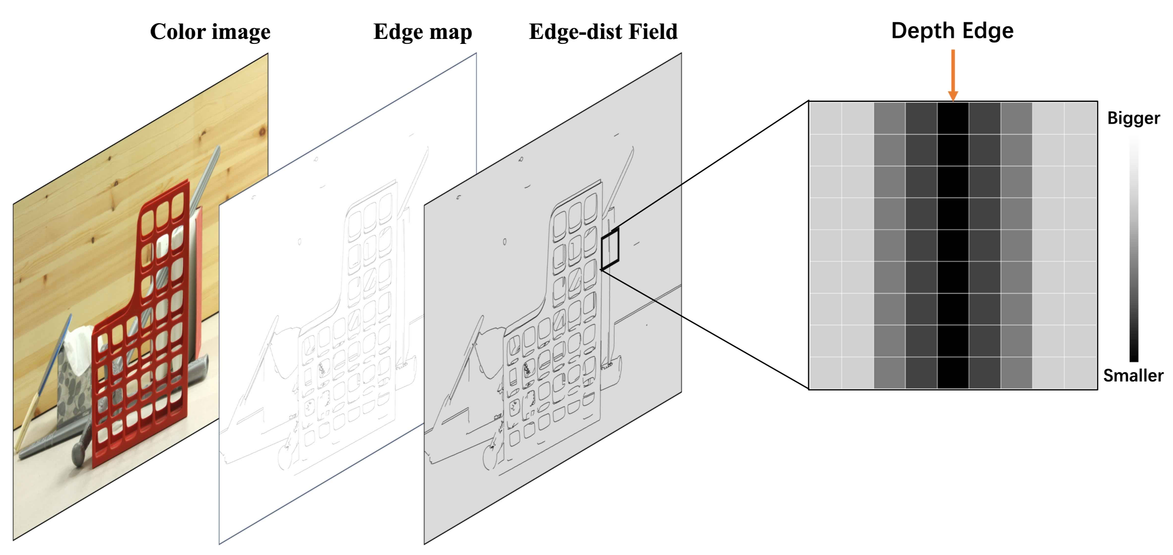
Figure 2: Process of obtaining continuous edge-dist field

Depth map mainly contains smooth regions separated by small amounts of edges. Around the depth edge, there are always sudden change of depth value. Thus, we design a continuous edge distance field used to prevent the depth value from crossing the depth edge to facilitate upsampling. In order to make the depth values near the edge have less influence on the other side of the depth edge, we set smaller weights near that. For the edge map $P$, given a location $(i,j)$ which point $P_{i,j}$ is a depth edge, the rule of the edge-dist field $E$ is defined as:

$$\mathrm{E}_{i,j}\leqq\mathrm{E}_{i\pm 1,j}\leqq\mathrm{E}_{i\pm 2,j}\leqq\ldots\leqq\mathrm{E}_{i\pm k-1,j}\leqq\mathrm{E}_{i\pm k,j}\leqq\mathrm{E}_{max}$$ (1)

where $E_{i,j}$ is the edge-dist value of the depth edge point. As is shown in Figure 2, the minima in an edge-dist field are on the depth edges. From the depth edges, the value increases gradually to the maximum value $E_{max}$ in the edge-dist field. As the weight of data confidence, the $E_{i,j}$ and $E_{max}$ span:

$$\mathrm{E}_{i,j},\mathrm{E}_{max}\in[0,1]$$ (2)

Please note that the EGCL evaluates to a normalized convolution layer[27] when values $E$ of the edge-dist field are all $1$.

3.2 Edge Guided Convolutional Layer

Based on the edge-dist field defined above, we propose a novel convolution layer, the edge guided convolutional layer, which using data confidence to dealing sparse inputs and continuous edge-dist fields as the guidance of depth filling. The edge guided convolutional layer can replace standard convolutional layer in the CNN framework. An illustration of the edge guided convolutional layer is shown in Figure 3 .

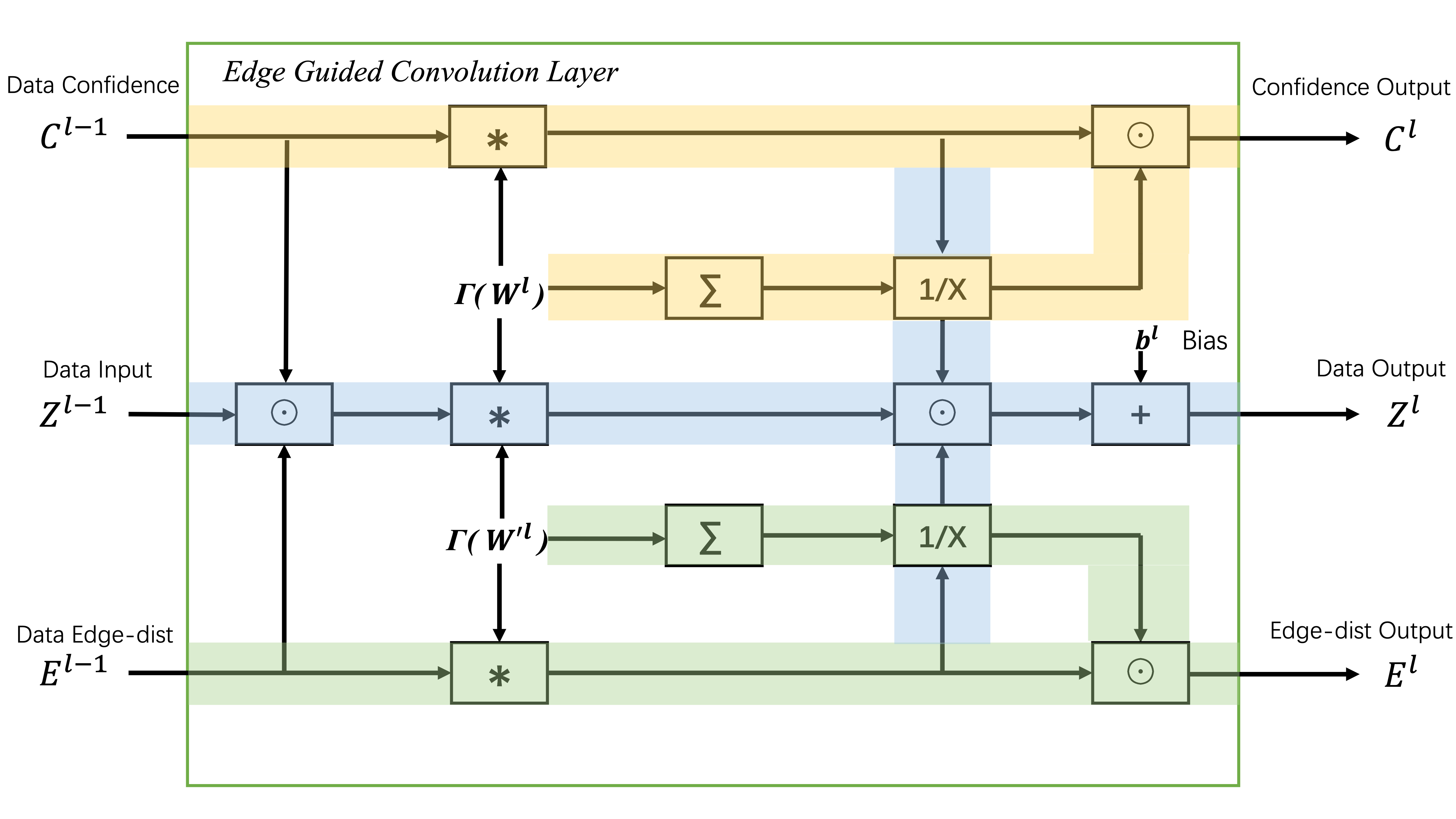
Figure 3: An illustration of the Edge Guided Convolutional layer that takes in three inputs: data, confidence and edge-dist. The Edge Guided Convolutional layer outputs a data term, a confidence term and an edge-dist term. Convolution is denoted as $\ast$, the Hadamard product (point-wise) as $\odot$, summation as $\sum$ , and point-wise inverse as 1/x.

First, the layer receives three inputs simultaneously, the sparse data, its confidence and edge-dist field. The forward pass is then modified according to 3, which is shown in Figure 3 as the blue area:

$$\mathbf{Z}_{i,j}^{l}=\frac{\sum_{m,n}\mathbf{Z}_{i+m,j+n}^{l-1}\mathbf{C}_{i+m,j+n}^{l-1}\mathbf{E}_{i+m,j+n}^{l-1}\Gamma\left(\mathbf{W}_{m,n}^{l}\right)}{\sum_{m,n}\mathbf{C}_{i+m,j+n}^{l-1}\mathbf{E}_{i+m,j+n}^{l-1}\Gamma\left(\mathbf{W}_{m,n}^{l}\right)+\epsilon}+\mathbf{b}^{l}$$ (3)

where $Z^{l}_{i,j}$ is the output of the $l^{th}$ layer at locations $i,j$ depending on the weight elements $W^{l}_{m,n}$, $Z^{l-1}$is the output data from the previous layer, $C^{l-1}$is the output confidence from the previous while $E^{l-1}$is the output edge-dist from the previous. $b^{l}$ is the bias and $\epsilon$ is a constant to prevent division by zero. Please note that this is formally a correlation, as it is a common notation in CNNs.

Similar to the method proposed in[46], our confidence output measure is shown in Figure 3 as the yellow area, which is defined as:

$$\mathbf{C}_{i,j}^{l}=\frac{\sum_{m,n}\mathbf{C}_{i+m,j+n}^{l-1}\Gamma\left(\mathbf{W}_{m,n}^{l}\right)+\epsilon}{\sum_{m,n}\Gamma\left(\mathbf{W}_{m,n}^{l}\right)}$$ (4)

As described in [36], using effective masks would degrade performance because masks in earlier layers in CNNs were saturated, which affects several methods in [9, 47, 35]. However, 4 allows propagating confidence between CNN layers without facing the above "validity mask saturation" problem.

To allow propagate edge-dist between CNN layers, as the same as what is illustrated in the yellow area of Figure 3, we define the edge-dist output measure as:

$$\mathbf{E}_{i,j}^{l}=\frac{\sum_{m,n}\mathbf{E}_{i+m,j+n}^{l-1}\Gamma\left(\mathbf{{W}^{\prime}}_{m,n}^{l}\right)+\epsilon}{\sum_{m,n}\Gamma\left(\mathbf{{W}^{\prime}}_{m,n}^{l}\right)}$$ (5)

where $E^{l-1}$is the output edge-dist from the previous layer, and ${{W}^{\prime}}^{l}_{m,n}$ is the specified weight elements, different from $W^{l}_{m,n}$ which is utilized in 4. In order to keep the consistency of the position of the edge information, ${{W}^{\prime}}^{l}_{m,n}$ is des igned as a filtering kernel which the intermediate element is 1 and 0 otherwise. This is expressed as:

$$\mathbf{{W}^{\prime}}_{i,j}^{l}=\left\{\begin{array}[]{ll}{1,}&{\text{ if }i=\lfloor m/2\rfloor,j=\lfloor n/2\rfloor}\\ {0,}&{\text{ otherwise }}\end{array}\right.$$ (6)

3.3 Depth Upsampling Network

The depth upsampling subnetwork is a common seven-layered convolutional neural network, but we replace all stand convolutional layers by our edge guided convolutional layers. The EGCLs in the depth upsampling subnetwork play two roles: on one hand, they are able to extract features directly from an irregularly sampled sparse depth map; on the other hand, the EGCLs also perform interpolation or upsampling for sparse data so that the produced feature maps are dense. The complete architecture of our network is illustrated in Figure 4.

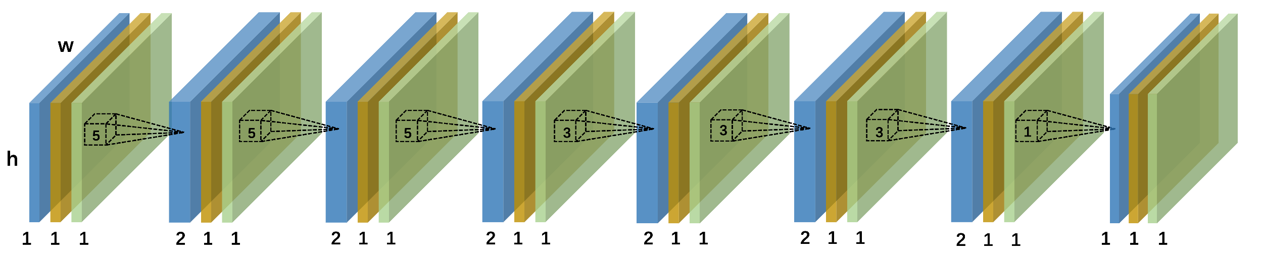
Figure 4: Our proposed depth upsampling network that utilizes Edge Guided Convolution layers. The input to our network is a sparse depth map (blue), a continuous confidence map (red) and a continuous edge-dist map (green). It passes through several Edge Guided Convolution layers (dashed) with decreasing kernel sizes from 5$\times$5 to 3$\times$3.

3.4 Fusion Network

Different edge extraction algorithms have their own limits and deficiencies, so do the dense depth images which guided by their different edge maps. The depth fusion subnetwork takes the weighted dense depth images from depth upsampling network which guided by different edge maps as the input. As is shown in Figure 5, the edge maps generated by the Canny operator (the upper threshold is 150, the lower threshold is 50, kernel size is 3) lose some depth edge details such as outline of cars compared with our handcrafted depth map(red rectangle in Figure 5). Although it contains much more details, the maps generated by the Canny operator (the upper threshold is 150, the lower threshold is 50, kernel size is 5) suffer from too much misleading edges made by textures on the object surface (yellow rectangle in Figure 5). These local dense edges will make the edge maps meaningless locally. So we design the fusion subnetwork. It can improve upsampling ability by combining multiple results guided by different edge maps into a single new result. It makes us to combine the advantages of different algorithms and achieve better performance.

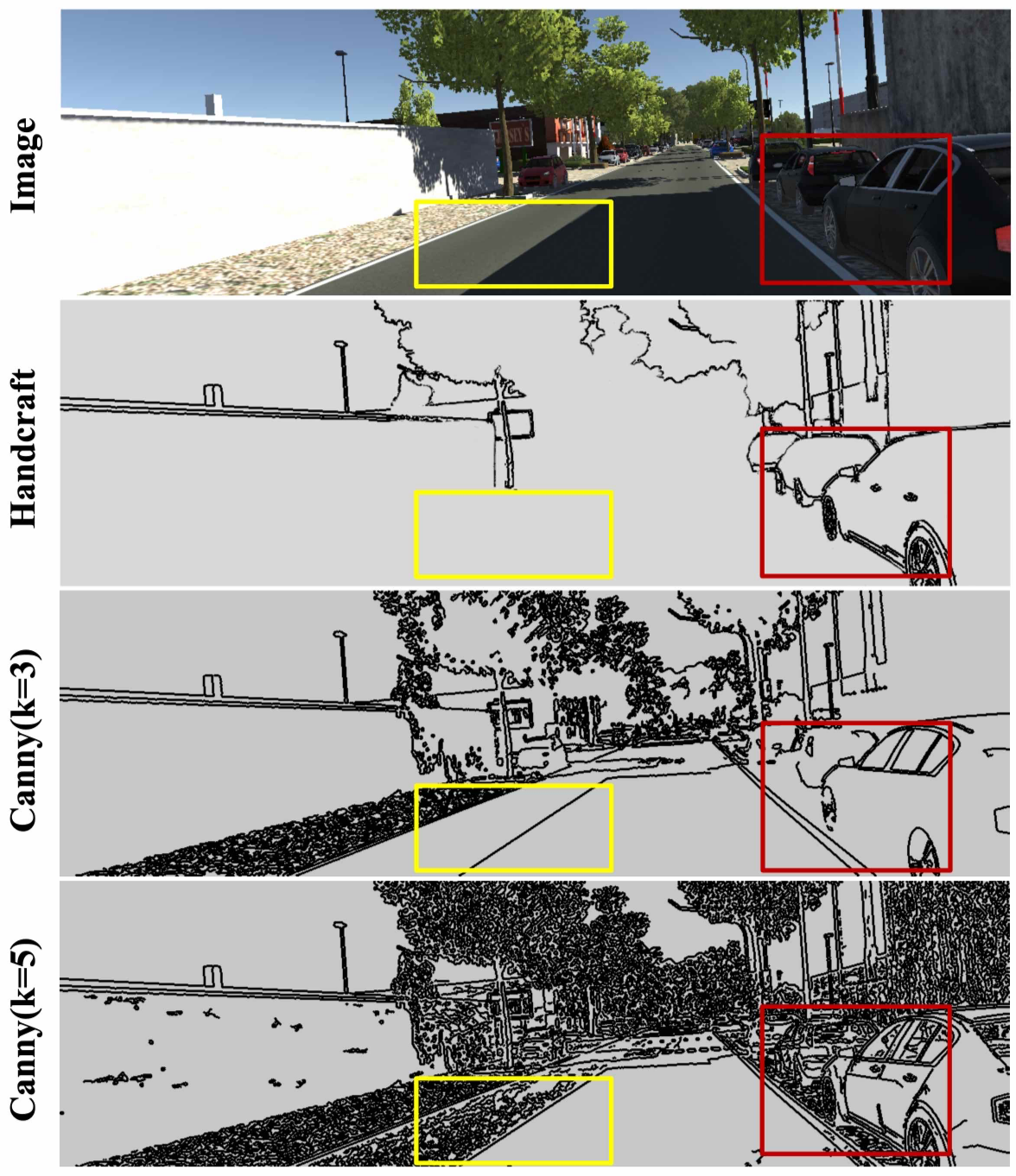
Figure 5: Qualitative comparison for different edge maps. Color image is shown in the top row. Our handcrafted depth map is ’Handcraft’. The edge map which generated by the Canny operator (the upper threshold is 150, the lower threshold is 50, kernel size is 3) is ’Canny(k=3)’, while ’Canny(k=5)’ is the edge map which generated by the Canny operator (the upper threshold is 150, the lower threshold is 50, kernel size is 5).

4 Experiments

To demonstrate the capabilities of our proposed approach, we evaluate our proposed networks on the Virtual KITTI [48] dataset and the Middlebury [44, 45]dataset for the task of sparse depth upsampling.

4.1 Datasets

Virtual KITTI is a photo-realistic synthetic video dataset designed to learn and evaluate computer vision models for several video understanding tasks.Virtual KITTI contains 50 high-resolution monocular videos (21,260 frames) generated from five different virtual worlds in urban settings under different imaging and weather conditions.These worlds were created using the Unity game engine and a novel real-to-virtual cloning method. These photo-realistic synthetic videos are at the pixel level with depth labels.

The Middlebury is a high-resolution stereo datasets of static indoor scenes with highly accurate ground-truth disparities. Please note that all the disparities images have been converted to depth images.

4.2 Experimental Setup

Both datasets provide us with dense depth maps and aligned color images. For experiments we synthetically generate sparse depth maps with different sampling rates by randomly sampling a percentage of points from the provided dense depth maps.

4.3 Evaluation Metrics

For the Virtual KITTI dataset, we compute the Mean Absolute Error (MAE) and the Root Mean Square Error (RMSE) on the depth values. The MAE is an unbiased error metric, takeing an average of the error across the whole image and it is defined as:

$$\operatorname{MAE(Z,T)}=\frac{1}{MN}\left[\sum_{i=0}^{N}\sum_{j=0}^{M}|Z(i,j)-T(i,j)|\right],$$ (7)

where $Z(i,j)$ is the data output from our method and $T(i,j)$is the data ground truth. The RMSE penalizes outliers and it is defined as:

$$\operatorname{RMSE(Z,T)}=\frac{1}{MN}\left[\sum_{i=0}^{N}\sum_{j=0}^{M}|Z(i,j)-T(i,j)|^{2}\right]^{1/2}.$$ (8)

Additionally, we also use iMAE and iRMSE, which are calculated on the disparity instead of the depth. The ’i’ indicates that disparity is proportional to the inverse of depth.

For the Middlebury dataset, we compute the RMSE, the MAE, and the inliers ratio $\delta_{i}$ as descriped in [49], which means the percentage of predicted pixels where the relative error is less a threshold $i$. Specifically, $i$ is chosen as 1.25,$1.25^{2}$ and $1.25^{3}$ separately for evaluation. Here, a higher $i$ indicates a softer constraint and a higher $\delta_{i}$ represents a better prediction. $\delta_{n}$ is defined as:

$$\delta_{n}=\frac{n\left(\left\{Z:\max\left\{\frac{Z}{T},\frac{T}{Z}\right\}<1.25^{n}\right\}\right)}{n\left(\left\{T\right\}\right)}$$ (9)

with n(·) as the cardinality of a set.

Table 1: Quantitative results on the Virtual KITTI dataset with the models trained at various sampling rates and tested at corresponding rates.(The best one is highlighted in bold.)

method	Samples	RMSE	MAE	iRMSE	iMAE
Sparse	5%	15.931	3.271	0.075	0.035
Normal		16.82	2.489	0.076	0.012
Edge(ours)		15.680	2.340	0.070	0.007
Sparse	0.8%	21.323	4.427	0.086	0.037
Normal		23.046	3.934	0.089	0.019
Edge(ours)		21.063	3.591	0.071	0.017
Sparse	0.2%	26.722	6.056	0.092	0.039
Normal		28.824	5.581	0.097	0.031
Edge(ours)		26.584	5.111	0.079	0.025

Table 2: Quantitative results on the Middlebury dataset with the models trained at various sampling rates and tested at corresponding rates.(The best one is highlighted in bold.)

method	samples	Lower the Better		Higher the Better
		RMSE	MAE	$\delta_{1}$	$\delta_{2}$	$\delta_{3}$
Sparse	5%	1.623	0.339	0.922	0.952	0.972
Normal		1.672	0.344	0.919	0.951	0.972
Edge(ours)		1.573	0.282	0.927	0.959	0.981
Sparse	0.8%	2.702	0.616	0.861	0.913	0.954
Normal		2.814	0.604	0.863	0.916	0.958
Edge(ours)		2.676	0.548	0.868	0.921	0.964
Sparse	0.2%	4.245	1.083	0.783	0.856	0.922
Normal		4.309	1.057	0.788	0.862	0.930
Edge(ours)		4.222	1.016	0.790	0.866	0.933

4.4 Evaluating Edge Guided Convolution Layer

We run a number of experiments to analyze our proposed convolution layer. To investigate the effectiveness of EGCL, we compare our models with those replacing EGCLs with either normalized convolutional layers[27] or sparse convolutional layers[9]. These models are, respectively, denoted using the suffixes ‘Edge’, ‘ Norm’ and ‘ Sparse’.

In experiments, to compare the performance on sparse data whose sampling rate is not more than 5%, we train all models at various sampling rates and test them at corresponding rates. Experiments are conducted on both datasets, from which consistent phenomena can be observed. We present the quantitative results on the Virtual KITTI dataset in Table 1 and the results on the Middlebury dataset in Table 2. The value in bold is the best.

Our model is improved on the basis of the normalized convolutional layer to generate sharper edges so that we can get less errors in the area around depth edges. From the tables, we can conclude that our method rank the first in the test results. Especially, at 5% sampling density, our MAE decreased by 28.5% and 16.8% on the Virtual KITTI dataset and the Middlebury dataset respectively.

Figure 6shows some qualitative results on the Virtual KITTI dataset while Figure 7 shows some on the Middlebury dataset. The predictions from ’Sparse’ and ’Normal’ are very blurry especially along depth edges. However,with the help of guidance by edge-dist field, our methods EGCL produce remarkably better reconstructions of the dense map, in particular with respect to edges sharpness and the level of details.

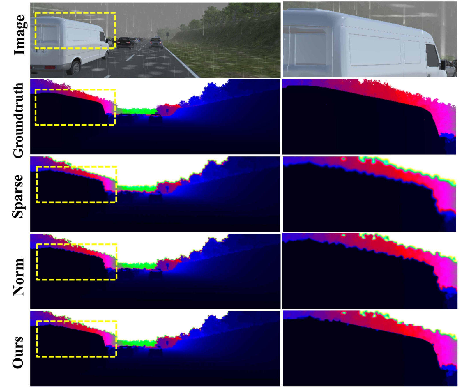
Figure 6: Qualitative comparison with state-of-the-art methods on the Virtual KITTI dataset under the ’rain’ conditions. The depth images are colorized along with depth range. Our results are shown in the bottom row and compared with top-ranking methods ‘Sparse’[9], ‘Normal’[27]. In the zoomed regions, our method preserves sharper edges.

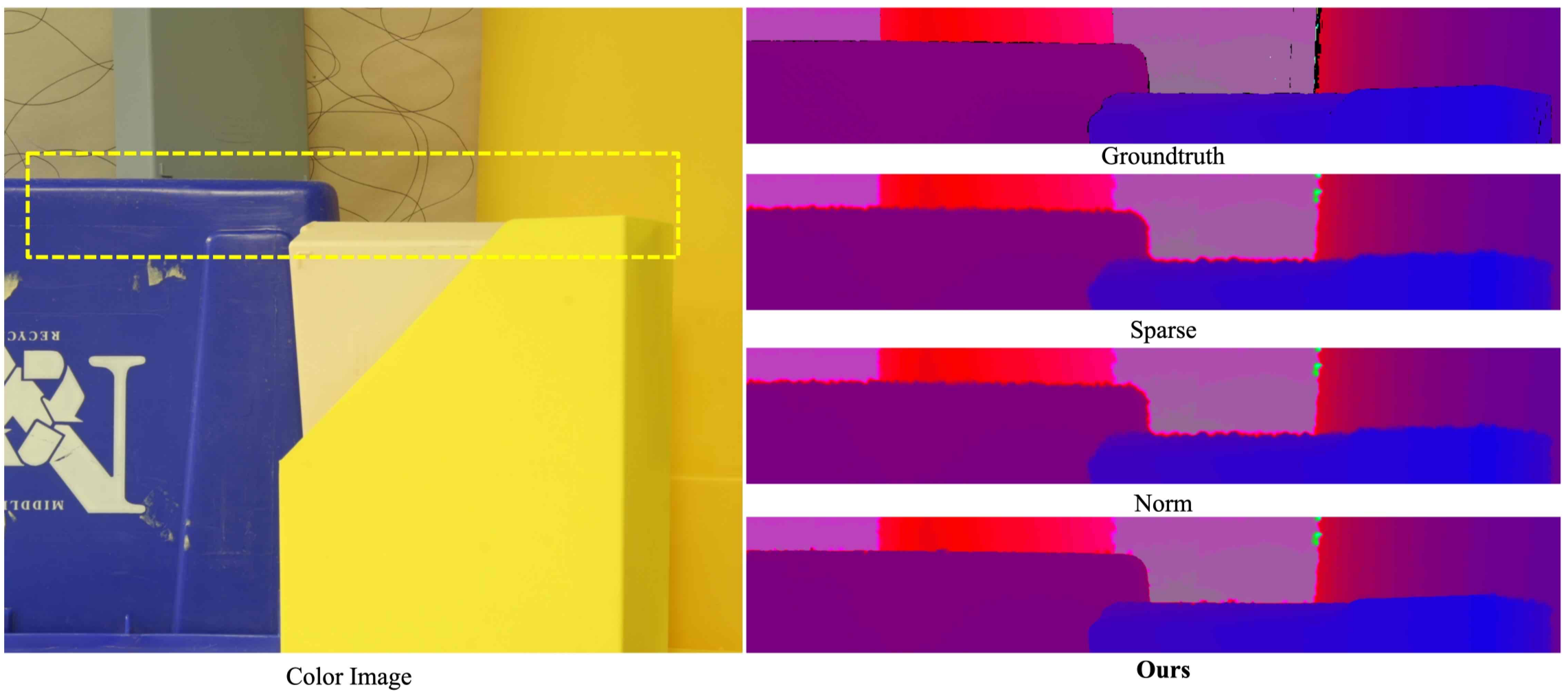
Figure 7: Qualitative comparison with state-of-the-art methods on the Middlebury dataset image ’Plastic’. The depth images are colorized along with depth range. Our results are shown in the bottom row and compared with top-ranking methods ‘Sparse’[9], ‘Normal’[27]. In the zoomed regions, our method recovers better 3D details.

4.5 Evaluating Edge Guided CNNs

To investigate the effectiveness of EGCNN, we then compare our full model EGCNN-Full to other ablation network structure which do not have fusion subnetwork, denoted as EGCNN-Ablations. Among them, the ablation network which use Canny(the upper threshold is 150, the lower threshold is 50,kernel size is 3) as the edge extraction algorithm is EGCNN-Ablation(k=3), while EGCNN-Ablation(k=5) uses Canny(the upper threshold is 150, the lower threshold is 50, kernel size is 5). Table 3 and 4 report the experimental results at five sampling rates (5%, 0.8%, 0.2%) on both datasets. As the same as the above, experiments are trained and tested at the same rate.

From Table 3 and 4 we get the following observations: (1)In most cases, EGCNN-Ablation(k=5) achieve better results than EGCNN-Ablation(k=3). As we can see in Figure 5, although there are more useful details in ’Canny(k=5)’, it do contains much more wrong edge information even very dense misleading edge lines. Quantitative experimental results show that wrong edge information can hardly make the performance of EGCL wrose but correct edge information do improve it. (2) With the help of fusion subnetwork, EGCNN-Full can combine the advantages of different edge extraction algorithms and achieve further better performance. Both tables show that our proposed model outperforms both ablation models in most cases, especially in RMSE.

Table 3: Quantitative results on the Vkitti dataset with the models trained at various sampling rates and tested at corresponding rates.(The best one is highlighted in bold.)

method	Samples	RMSE	MAE	iRMSE	iMAE
EGCNN-Ablation(k3)	5%	15.680	2.340	0.070	0.007
EGCNN-Ablation(k5)		15.674	2.338	0.069	0.007
EGCNN-Full		15.574	2.336	0.068	0.006
EGCNN-Ablation(k3)	0.8%	21.063	3.591	0.071	0.017
EGCNN-Ablation(k5)		21.056	3.596	0.070	0.017
EGCNN-Full		20.921	3.590	0.069	0.017
EGCNN-Ablation(k3)	0.2%	26.584	5.111	0.079	0.025
EGCNN-Ablation(k5)		26.577	5.111	0.077	0.026
EGCNN-Full		26.536	5.106	0.076	0.025

Table 4: Quantitative results on the Middleburry dataset with the models trained at various sampling rates and tested at corresponding rates.(The best one is highlighted in bold.)

method	samples	Lower the Better		Higher the Better
		RMSE	MAE	$\delta_{1}$	$\delta_{2}$	$\delta_{3}$
EGCNN-Ablation(k3)	5%	1.573	0.282	0.927	0.959	0.981
EGCNN-Ablation(k5)		1.571	0.281	0.933	0.977	1.000
EGCNN-Full		1.559	0.280	0.942	0.974	0.996
EGCNN-Ablation(k3)	0.8%	2.676	0.548	0.868	0.921	0.964
EGCNN-Ablation(k5)		2.669	0.549	0.860	0.913	0.955
EGCNN-Full		2.655	0.548	0.869	0.911	0.957
EGCNN-Ablation(k3)	0.2%	4.222	1.016	0.790	0.866	0.933
EGCNN-Ablation(k5)		4.208	1.014	0.781	0.861	0.934
EGCNN-Full		4.190	1.014	0.803	0.881	0.942

5 Conclusion

We propose a guided convolutional layer to recover dense depth from sparse and irregular depth image with an depth edge image as guidance. Our novel guided network can prevent the depth value from crossing the depth edge to facilitate upsampling.

We further design a convolution network based on proposed convolutional layer to combine the advantages of different algorithms and achieve better performance.

Extensive experiments and ablation studies verify the superior performance of our guided convolutional layer and the effectiveness of the convolution network on sparse depth upsampling. Our method not only shows strong results on both indoor and outdoor, virtual and realistic scenes, but also presents strong generalization capability under different point densities, various lighting and weather conditions. While this paper specifically focuses on the problem of sparse depth upsampling, we believe that other tasks in computer vision involving image edges can also benefit from the design of our edge guided convolution layer and the convolution network in this paper.

References

- [1] Velodyne. http://velodynelidar.com/hdl-64e.html, 2018.
- [2] Zetong Yang, Yanan Sun, Shu Liu, Xiaoyong Shen, and Jiaya Jia. Std: Sparse-to-dense 3d object detector for point cloud. In Proceedings of the IEEE International Conference on Computer Vision, pages 1951–1960, 2019.
- [3] Ming Liang, Bin Yang, Yun Chen, Rui Hu, and Raquel Urtasun. Multi-task multi-sensor fusion for 3d object detection. In Proceedings of the IEEE Conference on Computer Vision and Pattern Recognition, pages 7345–7353, 2019.
- [4] Xinxin Du, Marcelo H Ang, Sertac Karaman, and Daniela Rus. A general pipeline for 3d detection of vehicles. In 2018 IEEE International Conference on Robotics and Automation (ICRA), pages 3194–3200. IEEE, 2018.
- [5] Charles R Qi, Wei Liu, Chenxia Wu, Hao Su, and Leonidas J Guibas. Frustum pointnets for 3d object detection from rgb-d data. In Proceedings of the IEEE Conference on Computer Vision and Pattern Recognition, pages 918–927, 2018.
- [6] Luca Caltagirone, Mauro Bellone, Lennart Svensson, and Mattias Wahde. Lidar–camera fusion for road detection using fully convolutional neural networks. Robotics and Autonomous Systems, 111:125–131, 2019.
- [7] Zhe Chen, Jing Zhang, and Dacheng Tao. Progressive lidar adaptation for road detection. IEEE/CAA Journal of Automatica Sinica, 6(3):693–702, 2019.
- [8] Gernot Riegler, Matthias Rüther, and Horst Bischof. Atgv-net: Accurate depth super-resolution. In European conference on computer vision, pages 268–284. Springer, 2016.
- [9] Jonas Uhrig, Nick Schneider, Lukas Schneider, Uwe Franke, Thomas Brox, and Andreas Geiger. Sparsity invariant cnns. In 2017 International Conference on 3D Vision (3DV), pages 11–20. IEEE, 2017.
- [10] Carlo Tomasi and Roberto Manduchi. Bilateral filtering for gray and color images. In Sixth international conference on computer vision (IEEE Cat. No. 98CH36271), pages 839–846. IEEE, 1998.
- [11] Georg Petschnigg, Richard Szeliski, Maneesh Agrawala, Michael Cohen, Hugues Hoppe, and Kentaro Toyama. Digital photography with flash and no-flash image pairs. ACM transactions on graphics (TOG), 23(3):664–672, 2004.
- [12] James Diebel and Sebastian Thrun. An application of markov random fields to range sensing. In Advances in neural information processing systems, pages 291–298, 2006.
- [13] Jaesik Park, Hyeongwoo Kim, Yu-Wing Tai, Michael S Brown, and Inso Kweon. High quality depth map upsampling for 3d-tof cameras. In 2011 International Conference on Computer Vision, pages 1623–1630. IEEE, 2011.
- [14] Gernot Riegler, David Ferstl, Matthias Rüther, and Horst Bischof. A deep primal-dual network for guided depth super-resolution. arXiv preprint arXiv:1607.08569, 2016.
- [15] Tak-Wai Hui, Chen Change Loy, and Xiaoou Tang. Depth map super-resolution by deep multi-scale guidance. In European conference on computer vision, pages 353–369. Springer, 2016.
- [16] Yijun Li, Jia-Bin Huang, Narendra Ahuja, and Ming-Hsuan Yang. Deep joint image filtering. In European Conference on Computer Vision, pages 154–169. Springer, 2016.
- [17] Derek Chan, Hylke Buisman, Christian Theobalt, and Sebastian Thrun. A noise-aware filter for real-time depth upsampling. 2008.
- [18] Jennifer Dolson, Jongmin Baek, Christian Plagemann, and Sebastian Thrun. Upsampling range data in dynamic environments. In 2010 IEEE Computer Society Conference on Computer Vision and Pattern Recognition, pages 1141–1148. IEEE, 2010.
- [19] Johannes Kopf, Michael F Cohen, Dani Lischinski, and Matt Uyttendaele. Joint bilateral upsampling. In ACM Transactions on Graphics (ToG), volume 26, page 96. ACM, 2007.
- [20] Ming-Yu Liu, Oncel Tuzel, and Yuichi Taguchi. Joint geodesic upsampling of depth images. In Proceedings of the IEEE conference on computer vision and pattern recognition, pages 169–176, 2013.
- [21] Qingxiong Yang, Ruigang Yang, James Davis, and David Nistér. Spatial-depth super resolution for range images. In 2007 IEEE Conference on Computer Vision and Pattern Recognition, pages 1–8. IEEE, 2007.
- [22] Jonathan T Barron and Ben Poole. The fast bilateral solver. In European Conference on Computer Vision, pages 617–632. Springer, 2016.
- [23] David Ferstl, Christian Reinbacher, Rene Ranftl, Matthias Rüther, and Horst Bischof. Image guided depth upsampling using anisotropic total generalized variation. In Proceedings of the IEEE International Conference on Computer Vision, pages 993–1000, 2013.
- [24] Simon Hawe, Martin Kleinsteuber, and Klaus Diepold. Dense disparity maps from sparse disparity measurements. In 2011 International Conference on Computer Vision, pages 2126–2133. IEEE, 2011.
- [25] Nick Schneider, Lukas Schneider, Peter Pinggera, Uwe Franke, Marc Pollefeys, and Christoph Stiller. Semantically guided depth upsampling. In German Conference on Pattern Recognition, pages 37–48. Springer, 2016.
- [26] Xibin Song, Yuchao Dai, and Xueying Qin. Deep depth super-resolution: Learning depth super-resolution using deep convolutional neural network. In Asian conference on computer vision, pages 360–376. Springer, 2016.
- [27] Abdelrahman Eldesokey, Michael Felsberg, and Fahad Shahbaz Khan. Confidence propagation through cnns for guided sparse depth regression. IEEE transactions on pattern analysis and machine intelligence, 2019.
- [28] Hsieh Hou and H Andrews. Cubic splines for image interpolation and digital filtering. IEEE Transactions on acoustics, speech, and signal processing, 26(6):508–517, 1978.
- [29] Jianchao Yang, John Wright, Thomas S Huang, and Yi Ma. Image super-resolution via sparse representation. IEEE transactions on image processing, 19(11):2861–2873, 2010.
- [30] Chao Dong, Chen Change Loy, Kaiming He, and Xiaoou Tang. Image super-resolution using deep convolutional networks. IEEE transactions on pattern analysis and machine intelligence, 38(2):295–307, 2015.
- [31] Jiwon Kim, Jung Kwon Lee, and Kyoung Mu Lee. Accurate image super-resolution using very deep convolutional networks. In Proceedings of the IEEE conference on computer vision and pattern recognition, pages 1646–1654, 2016.
- [32] Ryan Dahl, Mohammad Norouzi, and Jonathon Shlens. Pixel recursive super resolution. In Proceedings of the IEEE International Conference on Computer Vision, pages 5439–5448, 2017.
- [33] Fangchang Ma, Guilherme Venturelli Cavalheiro, and Sertac Karaman. Self-supervised sparse-to-dense: Self-supervised depth completion from lidar and monocular camera. In 2019 International Conference on Robotics and Automation (ICRA), pages 3288–3295. IEEE, 2019.
- [34] Nathaniel Chodosh, Chaoyang Wang, and Simon Lucey. Deep convolutional compressed sensing for lidar depth completion. In Asian Conference on Computer Vision, pages 499–513. Springer, 2018.
- [35] Jiashen Hua and Xiaojin Gong. A normalized convolutional neural network for guided sparse depth upsampling. In IJCAI, pages 2283–2290, 2018.
- [36] Maximilian Jaritz, Raoul De Charette, Emilie Wirbel, Xavier Perrotton, and Fawzi Nashashibi. Sparse and dense data with cnns: Depth completion and semantic segmentation. In 2018 International Conference on 3D Vision (3DV), pages 52–60. IEEE, 2018.
- [37] Paolo Favaro. Recovering thin structures via nonlocal-means regularization with application to depth from defocus. In 2010 IEEE Computer Society Conference on Computer Vision and Pattern Recognition, pages 1133–1140. IEEE, 2010.
- [38] Sascha Wirges, Björn Roxin, Eike Rehder, Tilman Kühner, and Martin Lauer. Guided depth upsampling for precise mapping of urban environments. In 2017 IEEE Intelligent Vehicles Symposium (IV), pages 1140–1145. IEEE, 2017.
- [39] Yosuke Konno, Yusuke Monno, Daisuke Kiku, Masayuki Tanaka, and Masatoshi Okutomi. Intensity guided depth upsampling by residual interpolation. In The Abstracts of the international conference on advanced mechatronics: toward evolutionary fusion of IT and mechatronics: ICAM 2015.6, pages 1–2. The Japan Society of Mechanical Engineers, 2015.
- [40] Zixuan Huang, Junming Fan, Shuai Yi, Xiaogang Wang, and Hongsheng Li. Hms-net: Hierarchical multi-scale sparsity-invariant network for sparse depth completion. arXiv preprint arXiv:1808.08685, 2018.
- [41] Yinda Zhang and Thomas Funkhouser. Deep depth completion of a single rgb-d image. In Proceedings of the IEEE Conference on Computer Vision and Pattern Recognition, pages 175–185, 2018.
- [42] Jiaxiong Qiu, Zhaopeng Cui, Yinda Zhang, Xingdi Zhang, Shuaicheng Liu, Bing Zeng, and Marc Pollefeys. Deeplidar: Deep surface normal guided depth prediction for outdoor scene from sparse lidar data and single color image. In Proceedings of the IEEE Conference on Computer Vision and Pattern Recognition, pages 3313–3322, 2019.
- [43] Xinchen Ye, Xiangyue Duan, and Haojie Li. Depth super-resolution with deep edge-inference network and edge-guided depth filling. In 2018 IEEE International Conference on Acoustics, Speech and Signal Processing (ICASSP), pages 1398–1402. IEEE, 2018.
- [44] Daniel Scharstein and Richard Szeliski. A taxonomy and evaluation of dense two-frame stereo correspondence algorithms. International journal of computer vision, 47(1-3):7–42, 2002.
- [45] Daniel Scharstein, Heiko Hirschmüller, York Kitajima, Greg Krathwohl, Nera Nešić, Xi Wang, and Porter Westling. High-resolution stereo datasets with subpixel-accurate ground truth. In German conference on pattern recognition, pages 31–42. Springer, 2014.
- [46] Abdelrahman Eldesokey, Michael Felsberg, and Fahad Shahbaz Khan. Propagating confidences through cnns for sparse data regression. arXiv preprint arXiv:1805.11913, 2018.
- [47] Guilin Liu, Fitsum A Reda, Kevin J Shih, Tingchun Wang, Andrew Tao, and Bryan Catanzaro. Image inpainting for irregular holes using partial convolutions. pages 89–105, 2018.
- [48] A Gaidon, Q Wang, Y Cabon, and E Vig. Virtual worlds as proxy for multi-object tracking analysis. In CVPR, 2016.
- [49] David Eigen, Christian Puhrsch, and Rob Fergus. Depth map prediction from a single image using a multi-scale deep network. In Advances in neural information processing systems, pages 2366–2374, 2014.