The path to Z And-type outbursts: The case of V426 Sagittae (HBHA 1704-05)

Abstract

Context. The star V426 Sge (HBHA 1704-05), originally classified as an emission-line object and a semi-regular variable, brightened at the beginning of August 2018, showing signatures of a symbiotic star outburst.

Aims. We aim to confirm the nature of V426 Sge as a classical symbiotic star, determine the photometric ephemeris of the light minima, and suggest the path from its 1968 symbiotic nova outburst to the following 2018 Z And-type outburst.

Methods. We re-constructed an historical light curve (LC) of V426 Sge from approximately the year 1900, and used original low- (R$\sim$500–1 500; 330–880 nm) and high-resolution (R$\sim$11 000–34 000; 360–760 nm) spectroscopy complemented with Swift-XRT and UVOT, optical $UBVR_{\rm C}I_{\rm C}$ and near-infrared $JHKL$ photometry obtained during the 2018 outburst and the following quiescence.

Results. The historical LC reveals no symbiotic-like activity from $\sim$1900 to 1967. In 1968, V426 Sge experienced a symbiotic nova outburst that ceased around 1990. From approximately 1972, a wave-like orbitally related variation with a period of $493.4\pm 0.7$ days developed in the LC. This was interrupted by a Z And-type outburst from the beginning of August 2018 to the middle of February 2019. At the maximum of the 2018 outburst, the burning white dwarf (WD) increased its temperature to $\ga 2\times 10^{5}$ K, generated a luminosity of $\sim 7\times 10^{37}\,(d/3.3\,{\rm kpc})^{2}$$\rm\,erg\,s^{-1}$  and blew a wind at the rate of $\sim 3\times 10^{-6}$ $M_{\sun}\,{\rm yr}^{-1}$. Our spectral energy distribution models from the current quiescent phase reveal that the donor is a normal M4-5 III giant characterised with $T_{\rm eff}\sim 3\,400$ K, $R_{\rm G}\sim 106\,(d/3.3\,{\rm kpc})$ $R_{\sun}$ and $L_{\rm G}\sim 1350\,(d/3.3\,{\rm kpc})^{2}$ $L_{\sun}$ and the accretor is a low-mass $\sim$0.5 $M_{\sun}$ WD.

Conclusions. During the transition from the symbiotic nova outburst to the quiescent phase, a pronounced sinusoidal variation along the orbit develops in the LC of most symbiotic novae. The following eventual outburst is of Z And-type, when the accretion by the WD temporarily exceeds the upper limit of the stable burning. At this point the system becomes a classical symbiotic star.

1 Introduction

Symbiotic stars are the widest interacting binaries. Their orbital periods run from hundreds of days to a few tens or even hundreds of years, or are unknown (e.g. Belczyński et al. 2000; Parimucha et al. 2002; Schmid & Schild 2002; Matthews & Karovska 2006). This type of binary consists of a cool giant as the donor star and a white dwarf (WD), accreting from the giant’s wind (e.g. Boyarchuk 1967; Kenyon 1986; Mürset & Schmid 1999). The accretion process heats up the WD to $\ga 10^{5}$ K and increases its luminosity to $\sim 10^{1}-10^{4}$ $L_{\sun}$ (Mürset et al. 1991; Skopal 2005a), which ionises a fraction of the wind from the giant giving rise to the nebular emission (e.g. Boyarchuk et al. 1966; Seaquist et al. 1984; Nussbaumer & Vogel 1987). This configuration represents the so-called quiescent phase, during which symbiotic systems releases their energy at an approximately constant rate and spectral energy distribution (SED). The presence of an extended and partially optically thick nebula in the rotating binary gives rise to the wave-like variation of the light as a function of the orbital phase, which represents the most distinctive feature in the light curves (LCs) of symbiotic stars during their quiescent phases (see Skopal 2001; Sekeráš et al. 2019, and references therein). In most cases, high luminosities of a few times $10^{3}$ $L_{\sun}$ are generated by stable hydrogen burning on the WD surface at accretion rates of a few times ($10^{-8}-10^{-7})$ $M_{\sun}\,{\rm yr}^{-1}$, depending on the WD mass (e.g. Paczyński & Żytkow 1978; Shen & Bildsten 2007). In some cases we measure low luminosities of $\sim 10^{1}-10^{2}$ $L_{\sun}$, which are generated by the accretion process onto the WD, when its gravitational potential energy is converted into radiation by the disc (e.g. Pringle 1981).

Sometimes, symbiotic systems undergo outbursts indicated by brightening of a few magnitudes in the optical. Outbursts, resulting from a prolonged accretion by the WD until ignition of a thermonuclear event, can be grouped into two classes: (i) The symbiotic nova outbursts occur when the nuclear burning at the WD surface turns on in non-degenerate conditions, is non-explosive, and proceeds in thermal equilibrium (see Fujimoto 1982a, b). The LC is characterised by a moderate amplitude (a few magnitudes) and slow (a few years) rise to maximum and long duration (from decades to centuries or more). More details can be found in Allen (1980), Munari (1997), Mürset & Nussbaumer (1994), and Munari (2019). (ii) The other class occur when the material is accreting onto the WD under degenerate conditions, and the thermonuclear outburst is explosive. The outburst reaches peak luminosity within a few minutes, ejects a large amount of mass at high velocities, and lasts for weeks or months. If the accretion runs at a high rate onto a massive WD, a thermonuclear outburst can be recorded more than once during the history of observations. These events are called recurrent (symbiotic) novae (e.g. Bode & Evans 2008; Starrfield et al. 2016, for a review). Finally, there are ‘Z-And type’ outbursts that can result from an increase in the accretion rate above that sustaining the stable burning, which leads to expansion of the burning envelope simulating an A–F type pseudophotosphere (e.g. Paczyński & Rudak 1980) and/or blowing optically thick wind from the WD (Hachisu et al. 1996). The latter was recently demonstrated for the 2015 outburst of AG Peg (Skopal et al. 2017). This type of outburst shows 1–3 mag brightening in the optical evolving on a timescale of weeks to years, often prolonged with multiple re-brightenings (see e.g. Fig. 1 of Skopal et al. 2018), and signatures of enhanced mass outflow (e.g. Fernández-Castro et al. 1995). This stage is called the active phase of the symbiotic binary.

Based on disentangling the composite continuum of symbiotic stars, Skopal (2005a) classified Z And-type outbursts into two classes depending on the orbital inclination: Systems with a high orbital inclination show the 1st-type outburst; their spectra consist of a low-temperature ($1-2\times 10^{4}$ K) warm pseudophotosphere and a strong nebular continuum. Systems with a low orbital inclination exhibit the 2nd-type outburst; their spectra consist of a high-temperature ($\approx 165\,000$ K) stellar component and a strong nebular continuum. This classification is based on a disc-like structure around the burning WD created during Z And-type outbursts at the orbital plane (Skopal 2005a; Cariková & Skopal 2012). The flared outer rim of the disc (which is the warm pseudophotosphere) then occults the central ionising source on the line of sight for systems with a high orbital inclination, which gives rise to the spectrum observed during the 1st-type outbursts. On the other hand, for low-inclination systems we can directly see the hot central source, and thus measure spectrum with characteristics of the 2nd-type outbursts. The nebula above and below the disc is observable in both cases.

The star V426 Sge (see Kazarovets et al. 2019, for the given name) was originally classified as an emission-line star HBHA 1704-05 by Kohoutek & Wehmeyer (1999). Based on measurements obtained within The All Sky Automated Survey for SuperNovae (ASASSN, see Shappee et al. 2014; Jayasinghe et al. 2018), the object was catalogued in the Variable Star Index as a semi-regular variable with a periodicity of around 418 days. According to ”Transient Object Followup Reports” of CBAT the star TCP J19544251+1722281 brightened from $V=12.0$ on July 31.945, 2018, to $V=10.7$ on August 8.938, 2018. The brightening was confirmed by the ASASSN measurements for the SR variable ASASSN-V J195442.95+172212.6 as a possible symbiotic star in outburst. On August 11, 2018, Munari et al. (2018) reported that both these stars are coincident with the position of HBHA 1704-05, a symbiotic star undergoing a ‘hot-type’ outburst.

Here, we explore the historical LC of V426 Sge, determine characteristics of its 2018 outburst and, with the aid of similar behaviour of other symbiotic novae, we suggest the path from the symbiotic nova outburst to the first Z And-type outburst. For this purpose, we re-construct the historical LC from approximately the year 1900 to the present and use our high-cadence optical spectroscopy complemented with Swift-XRT and UVOT, optical $UBVR_{\rm C}I_{\rm C}$ and near-infrared (NIR) $JHKL$ photometry. We introduce our observations in Sect. 2. We describe our analysis and present our results in Sect. 3. A discussion and summary are found in Sects. 4 and 5, respectively.

Table 1: Log of Swift-XRT observations of V426 Sge during its 2018 outburst and following quiescent phase. Count rates and fluxes are in 10^-3cts s^-1 and 10^-13$\rm\,erg\,s^{-1}\,cm^{-2}$, respectively (see Sect. 2.1.1).

Date	$T_{\rm start}$	$t_{\rm exp}$	Count-rate	Flux
	(UT)	(ks)
Aug. 28, 2018	17:03	1.0	15.6$\pm$4.9	3.7$\pm$1.2
Sep. 11, 2018	10:47	0.8	9.7$\pm$4.2	2.3$\pm$1.0
Sep. 18, 2018	02:23	1.1	12.0$\pm$3.8	2.9$\pm$0.9
Oct. 06, 2018	10:25	2.0	6.7$\pm$2.2	1.6$\pm$0.5
Oct. 11, 2018	01:46	2.3	9.0$\pm$2.3	2.2$\pm$0.6
Mar. 03, 2019	04:18	2.8	$<$2.2	$<$0.6

Table 2: As in Table 1, but for Swift-UVOT observations and fluxes in 10^-14$\rm\,erg\,s^{-1}\,cm^{-2}\,\AA^{-1}$. The reported magnitudes are in the Vega system.

Filter	Date	$T_{\rm start}$	$t_{\rm exp}$	Mag.	Flux
		(UT)	(s)
UVW2	Aug. 28, 2018	17:19	81	11.49$\pm$0.03	13.6$\pm$0.4
UVW2	Sep. 11, 2018	10:50	800	11.77$\pm$0.02	10.5$\pm$0.2
UVW2	Sep. 18, 2018	02:25	1032	11.85$\pm$0.02	9.7$\pm$0.2
UVW2	Oct. 06, 2018	10:28	620	12.06$\pm$0.02	8.04$\pm$0.16
UVW2	Oct. 11, 2018	02:03	173	12.10$\pm$0.03	7.72$\pm$0.18
UVW2	Mar. 03, 2019	04:18	550	13.67$\pm$0.04	1.82$\pm$0.06
UVM2	Aug. 28, 2018	16:58	128	11.58$\pm$0.03	10.8$\pm$0.3
UVM2	Oct. 06, 2018	10:34	620	12.16$\pm$0.02	6.37$\pm$0.14
UVM2	Oct. 11, 2018	01:41	312	12.15$\pm$0.03	6.42$\pm$0.15
UVW1	Oct. 06, 2018	10:39	669	11.40$\pm$0.02	10.5$\pm$0.2

2 Observations and data reduction

2.1 Photometry

2.1.1 X-ray and ultraviolet observations with Swift

The Neil Gehrels Swift Observatory (Gehrels et al. 2004, hereafter Swift) observed the source V426 Sge in six instances between August 28, 2018, and March 3, 2019, with the XRay Telescope (Burrows et al. 2005, hereafter XRT) and the UltraViolet-Optical Telescope (Roming et al. 2005, hereafter UVOT). The XRT allows coverage of the 0.3-10 keV band, whereas UVOT data were collected using the ultraviolet filters UVW2 ($\lambda$ = 1928 Å), UVM2 ($\lambda$ = 2246 Å), and UVW1 ($\lambda$ = 2600 Å) (see Poole et al. 2008, in detail). In a few cases, multiple UVOT data in different filters were collected during the same XRT pointing.

All observations were reduced within the ftools environment (Blackburn 1995). The XRT data reduction was performed using the xrtdas standard data pipeline package (xrtpipeline v. 0.13.4) in order to produce screened event files. All data were extracted only in the photon counting (PC) mode (Hill et al. 2004) adopting the standard grade filtering (0-12 for PC) according to the XRT nomenclature, and using an extraction radius of 47^′′ (20 pixels) centred at the optical coordinates of the source.

The XRT count rates were then measured using the routines xselect and image assuming a threshold S/N=3 for the detections. The rate correction factors were determined using the xrtlccorr task. Although, the X-ray detections were at low significance (around 3-4$\sigma$), it was possible to recognise that the bulk of photons ($>$92%) falls below 2 keV.

X-ray fluxes were determined using the webpimms online tool. A crude spectral modelling for a bremsstrahlung emission with characteristic temperature $kT_{\rm br}<1$ keV or, alternatively, a blackbody spectrum with temperature $kT_{\rm bb}<0.35$ keV, imply a count rate-to-flux conversion factor of $\sim$2.4$\times$10^-11 erg cm^-2 s^-1 cts^-1. In modelling, we used a hydrogen column density corresponding to $E_{\rm B-V}=0.2$ mag (see the end of Sect. 2.2) according to the formula of Predehl & Schmitt (1995).

Count rates on the UVOT images at the position of V426 Sge were measured through aperture photometry using 5^′′ apertures, whereas the corresponding background was evaluated for each image using a combination of several circular regions in source-free nearby areas. The data were calibrated using the UVOT photometric system described by Poole et al. (2008). Table 1 lists timing and results of the XRT observations, while Table 2 introduces the same, but for the UVOT pointings.

2.1.2 Ground-based multicolour photometry

Table 4 summarises basic information about instrumentation used to obtain our optical $UBVR_{\rm C}I_{\rm C}$ and NIR $JHKL$ photometry during the 2018 outburst and the following quiescence, as well as the historical photographic LC re-constructed from approximately 1900 to 1995. Data are available in Tables 10, 11, 3, and 12. Photometric evolution of V426 Sge is shown in Fig. 1 and analysed in Sect. 3.1.

Multicolour photometry was also used to convert the relative and/or arbitrary fluxes of our spectra to absolute fluxes. To obtain photometric flux-points of the true continuum, we determined corrections for emission lines from our low-resolution spectra using the procedure of Skopal (2007). $UBV$ and $R_{\rm C}I_{\rm C}$ magnitudes were converted to fluxes according to the calibration of Henden & Kaitchuck (1982) and Bessel (1979), respectively.

Table 3: NIR $JHKL$ photometry of V426 Sge.

HJD	$J$	$H$	$K$	$L$
-2 458 000
655.5	7.95$\pm$0.01	7.01$\pm$0.01	6.69$\pm$0.00	6.37$\pm$0.03
656.4	7.94$\pm$0.01	7.00$\pm$0.01	6.69$\pm$0.00	6.35$\pm$0.03
678.5	7.89$\pm$0.01	7.01$\pm$0.01	6.64$\pm$0.01	6.36$\pm$0.03
707.4	7.84$\pm$0.01	6.91$\pm$0.01	6.60$\pm$0.01	6.32$\pm$0.04
720.4	7.84$\pm$0.01	6.91$\pm$0.01	6.59$\pm$0.01	6.29$\pm$0.02

Table 4: Log of observatories and instrumentations used to obtain our ground-based photometry.

Observatory	Telescope†	Detector	Filters	Reference⋆	Table
SLO,G2a	60	CCD: FLI ML3041	$U,B,V,R_{\rm C},I_{\rm C}$	1	10
SLO,G1b	18	CCD: SBIG ST-10 MXE	$B,V,R_{\rm C},I_{\rm C}$	1	10
ANS Collab.c	30, 40	CCD: SBIG ST-8, MG4-9000	$B,V,R_{\rm C},I_{\rm C}$	2,3	11
AOKSd	35.6	CCD: G2-1600	$B,V,R_{\rm C},I_{\rm C}$	4	10
SAIe	125	InSb photometer	$J,H,K,L$	5	3
SAI	40,16,50	photographic plate	$m_{\rm pg}$	6,7,8	12
SOf	30,40	photographic plate	$m_{\rm pg}$, $m_{\rm pv}$	6,7,8	12

Notes. ^(a) Stará Lesná Observatory – pavilion G2, ^(b) SLO – pavilion G1, ^(c) Asiago Novae and Symbiotic stars Collaboration, ^(d) Astronomical Observatory at the Kolonica Saddle, ^(e) Sternberg Astronomical Institute of the Moscow University, ^(f) Sonneberg Observatory archive: http://www.4pisysteme.de/observatory/observatory$\_$4$\_$2$\_$en.html. ^⋆ 1 – Sekeráš et al. (2019), 2 – Munari et al. (2012a), 3 – Munari & Moretti (2012b), 4 – Kudzej et al. (2019), 5 – Shenavrin et al. (2011), 6 – Bacher et al. (2005), 7 – Sokolovsky et al. (2016), 8 – http://scan.sai.msu.ru/vast/. ^† diameter of the primary mirror in cm.

Table 5: Log of observatories and instrumentations used to obtain our spectroscopic observations.

Observatory	Telescope†	Spectrograph	Camera	Res.‡	Observer	Reference⋆	Label∗
CrAOa	260	slit SPEM	SPEC-10	1000	Tarasova	1	(iv)
Asiagob	182	echelle	EEV CCD47-10	21000	Munari	2	(iii)
SPOc	130	echelle	Andor iKon-L 936	34000	Komžík, Sekeráš	3,4,5	(i)
Asiago	122	Boller&Chivens	Andor iDus DU440A	1000	Munari	6,7	(iii)
SLO,G1	60	echelle	ATIK 460EX	11000	Shugarov, Kundra	4	(ii)
Durtal	51	echelle	KAF-3200ME	11000	Charbonnel	8,9	(x)
la Tourbière	40	echelle	ATIK 460EX	11000	Garde	1,9	(viii)
DCOd	35	LISA	ATIK 460EX	1000	Sims	1,9	(xiii)
Mill Ridge	31	echelle	ASI 1600mm CMOS	12000	Lester	1,9	(ix)
AOKS	28	LISA	ATIK 460EX	680	Dubovský	10	(v)
CTOe	25	UVEX	SWO CMOS	1200	Buil	9,11	(vi)
OCT-FRf	20	slit Alpy 600	ATIK 314L+	500	Boussin	9	(vii)
L’Aquilag	20	slit Alpy 600	SBIG ST-8300M	1600	Sollecchia	9	(xi)
Balzarettoh	20	slit Alpy 600	SXVF-M7	530	Franco	9	(xii)

Notes. ^(a) Crimean Astrophysical Observatory, ^(b) Asiago Astrophysical Observatory, ^(c) Skalnaté Pleso Observatory, ^(d) private Desert Celestial Observatory in Gilbert Arizona, ^(e) Castanet Tolosan Observatory, ^(f) Observatory de l’Eridan, ^(g) private station in L’Aquila, ^(h) A81 Balzaretto Observatory. ^⋆ 1 – Skopal et al. (2017), 2 – Munari & Lattanzi (1992), 3 – Baudrand & Bohm (1992), 4 – Pribulla et al. (2015), 5 – Döhring et al. (2019), 6 – Ciroi et al. (2014), 7 – Siviero (2014), 8 – Skopal et al. (2014), 9 – Teyssier (2019), 10 – Kudzej & Dubovský (2014), 11 – http://www.astrosurf.com/buil/UVEX$\_$project$\_$us/. ^† diameter of the primary mirror in cm, ^‡ average resolution, ^∗ label of the observatory in Tables 6 and 7.

2.2 Spectroscopy

Spectroscopic observations were secured at 13 observatories and/or private stations. Basic information about instrumentation for the spectra acquisition is introduced in Table 5.

Low-resolution spectra (Table 6) were used to model the SED. Their flux calibration was verified with the aid of the near-simultaneous emission-line-free $UBVR_{\rm C}I_{\rm C}$ photometry. High- and medium-resolution spectra (Table 7) served to analyse variations in the line profiles and fluxes.

The distance of $3.3^{+0.7}_{-0.6}$ kpc was determined by Bailer-Jones et al. (2018) using the parallax of V426 Sge published in the second Gaia data release (Gaia Collaboration 2018). According to a 3D map of interstellar dust reddening published by Green et al. (2018), we estimated the colour excess $E_{\rm B-V}\sim 0.2$ mag in direction to V426 Sge for 3.3 kpc. Modelling the Swift-UVOT and optical continuum fluxes allowed us to specify the colour excess to $E_{\rm B-V}=0.2\pm 0.02$ mag (see Sect. 3.2.1), which, together with the extinction curve of Cardelli et al. (1989), we used to deredden our observations.

Table 6: Log of low-resolution spectroscopic observations

Datea	JD 2 4…	Range	$T_{\rm exp}$	Obs.b
yyyy/mm/dd.ddd		[nm]	[s]
2018/08/10.851	58341.351	330 - 788	120	(iii)
2018/08/10.878	58341.378	375 - 737	3649	(xi)
2018/08/10.932	58341.432	350 - 507	6167	(vi)
2018/08/11.915	58342.415	370 - 757	3926	(vii)
2018/08/11.972	58342.472	339 - 457	5495	(vi)
2018/08/15.888	58346.388	370 - 757	4532	(vii)
2018/08/18.896	58349.396	370 - 757	4833	(vii)
2018/08/19.895	58350.395	327 - 796	120	(iii)
2018/08/21.899	58352.399	330 - 757	1200	(iv)
2018/08/28.860	58359.360	383 - 723	3600	(xii)
2018/09/01.828	58363.328	330 - 757	1200	(iv)
2018/09/07.886	58369.386	370 - 757	4525	(vii)
2018/09/11.903	58373.403	370 - 757	3621	(vii)
2018/09/15.911	58377.411	370 - 757	3621	(vii)
2018/09/19.827	58381.327	336 - 580	9970	(vi)
2018/09/20.888	58382.388	330 - 788	120	(iii)
2018/09/22.808	58384.308	580 - 879	4266	(vi)
2018/09/28.911	58390.411	370 - 757	2109	(vii)
2018/10/07.712	58399.212	330 - 757	900	(iv)
2018/10/17.732	58409.232	330 - 757	1200	(iv)
2018/11/18.708	58441.208	333 - 803	120	(iii)
2018/12/08.681	58461.181	330 - 794	120	(iii)
2018/12/17.704	58470.204	370 - 791	120	(iii)
Quiescent phase
2019/06/23.872	58658.372	384 - 758	6000	(v)
2019/06/25.931	58660.431	384 - 758	6000	(v)
2019/08/19.832	58715.332	330 - 781	240	(iii)
2019/09/07.191	58733.691	371 - 730	3323	(xiii)
2019/10/05.112	58761.612	371 - 730	3994	(xiii)

Notes. ^(a) Start of the observation in UT, ^(b) label of the observatory from Table 5.

Table 7: Log of high-resolution spectroscopic observations

Datea	JD 2 4…	Range	$T_{\rm exp}$	Obs.b
yyyy/mm/dd.ddd		[nm]	[s]
2018/08/10.845	58341.345	420-759	10800	(viii)
2018/08/11.826	58342.326	420-759	12000	(viii)
2018/08/12.872	58343.372	580-720	2700	(i)
2018/08/13.814	58344.314	425-720	2700	(i)
2018/08/13.827	58344.327	392-710	3600	(ii)
2018/08/15.853	58346.353	420-759	12000	(viii)
2018/08/17.070	58347.570	403-795	9600	(ix)
2018/08/17.896	58348.396	392-710	3600	(ii)
2018/08/18.823	58349.323	392-710	3600	(ii)
2018/08/19.842	58350.342	392-710	3600	(ii)
2018/08/20.060	58350.560	403-795	10800	(ix)
2018/08/20.868	58351.369	425-720	3600	(i)
2018/08/22.833	58353.333	360-712	600	(iii)
2018/08/22.840	58353.340	425-720	4500	(i)
2018/08/27.796	58358.296	425-720	2700	(i)
2018/09/07.867	58369.367	425-720	3600	(i)
2018/09/19.821	58381.321	425-720	4500	(i)
2018/09/20.837	58382.337	425-720	4500	(i)
2018/09/20.882	58382.382	360-712	900	(iii)
2018/10/04.840	58396.340	392-710	3600	(ii)
2018/10/05.724	58397.224	392-710	5100	(ii)
2018/10/10.788	58402.288	392-710	4800	(ii)
2018/10/11.835	58403.335	392-710	6000	(ii)
2018/10/16.713	58408.213	425-720	5400	(i)
2018/10/18.797	58410.297	404-759	6159	(x)
2018/10/20.757	58412.257	360-712	600	(iii)
2018/11/08.741	58431.241	392-710	3600	(ii)
2018/11/10.773	58433.273	392-710	2700	(ii)
2018/11/12.803	58435.303	392-710	2400	(ii)
2018/11/23.729	58446.229	425-720	3600	(i)
2018/12/17.701	58470.201	360-711	900	(iii)
2019/11/13.760	58801.260	360-711	900	(iii)

Notes. ^(a) Start of the observation in UT, ^(b) label of the observatory from Table 5.

3 Analysis and results

3.1 Photometric evolution

Figure 1 shows the historical LC of V426 Sge from 1900 to the present that we measured on photographic plates (Table 12), supplemented with ASASSN $V$ magnitudes and our $UBVR_{\rm C}I_{\rm C}$ photometry (Sect. 2.1.2). The LC shows three particularly distinctive features: (i) a symbiotic nova outburst in 1968, (ii) development of wave-like orbitally related variations, and (iii) a Z And-type outburst in 2018. We describe these events as follows.

3.1.1 Symbiotic nova outburst in 1968

Photographic measurements revealed that the first recorded outburst started around 1967.5 from $m_{\rm pg}\sim 13.5$ and peaked around 1968.5 at $m_{\rm pg}\sim 11.5$ mag. After a 60-day decline by $\sim$0.5 mag, the star kept its brightness at $m_{\rm pg}\sim 12.0$ to approximately mid-1971, before a gradual decline to approximately 1990. During the decline, a pronounced wave-like variation developed in the LC (see panel b). We did not find this type of variability prior to the outburst, although the LC is well defined from 1928 to 1967 (Fig. 1). It is of interest to note that the same type of LC profile was observed for the symbiotic nova V1329 Cyg around its 1964 outburst: (i) No symbiotic-like variability prior to the outburst, (ii) a two-year brightening by 2–3 mag, followed by (iii) a gradual $\sim$20-year decline, during which periodic wave-like variations connected with the binary motion developed (see Figs. 4 and 5 of Skopal 1998, and Fig. 12 here). Similar evolution of the wave-like variability was also recorded in the LC of the symbiotic nova AG Peg during its decline from the 1850 outburst (Fig. 12). Accordingly, we classify the 1968 outburst of V426 Sge as a symbiotic nova outburst.

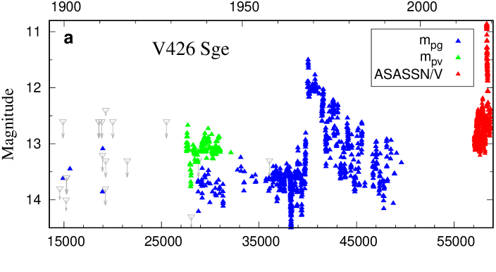
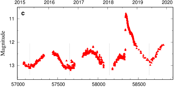
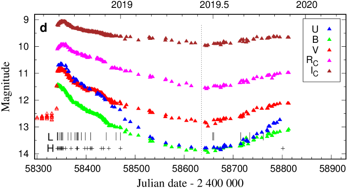
Figure 1: a: Historical LC of V426 Sge from 1900 to the present as given by our photographic m_pg/m_pv magnitudes (blue/green triangles), ASASSN and our $V$ magnitudes (red triangles). Grey triangles with arrows denote a limiting magnitude on plates with unseen target. b: Detail of the LC covering the 1968 symbiotic nova outburst. Decline from the maximum and wave-like periodic variation are denoted by the dotted and full line, respectively. c: The $V$-LC from 2015 to the present showing the ASASSN and our data. d: $UBVR_{\rm C}I_{\rm C}$ LCs covering the 2018 outburst and the present quiescence. Vertical bars and crosses denote the dates of our low (L) and high (H) resolution spectra. Dotted vertical lines in the panel c and d mark the light minima according to the ephemeris (1).

3.1.2 Wave-like orbitally related variation

The ASASSN $V$-LC, recorded from February 26, 2015, to July 30, 2018 (671 measurements), shows a wave-like variability with a period of $\sim$500 days (see panel c of Fig. 1). Using the Lafler-Kinnman algorithm (see Lafler & Kinman 1965), we determined the ephemeris of the light minima as, $JD_{\rm Min,\,V}=2\,456\,660(\pm 7)+494(\pm 5)\times E$. In the same way we analysed this type of variability in the $m_{\rm pg}$-LC during the transition from the 1968 outburst to quiescence. We obtained the ephemeris, $JD_{\rm Min,\,mpg}=2\,440\,872(\pm 10)+493.5(\pm 2.0)\times E$ using 309 magnitudes between July 29, 1971, and July 18, 1990, for which we subtracted their decline using a third-order polynomial (dotted line in panel b). Within the uncertainties, both ephemerides are identical in zero phase and period, which suggests a common origin of the wave-like variability in both colours. Analysing both datasets together, we obtained the ephemeris of the light minima as,

$$JD_{\rm Min}=2\,440\,873(\pm 7)+493.4(\pm 0.7)\times E.$$ (1)

Figure 2 shows the phase diagram of both the datasets plotted with the ephemeris (1). Their fits by sinusoidal curve determine amplitudes of the wave-like variations, $\Delta$$V\sim 0.66$ mag and $\Delta$$m_{\rm pg}\sim 0.94$ mag, which is the difference between the maximum and minimum. The corresponding colour index $m_{\rm pg}-V$ also varies with the phase, with a maximum around the phase $\varphi=0$ and a minimum around $\varphi=0.5$. These characteristics are typical for the orbitally related wave-like variability that develops during quiescent phases of symbiotic stars (e.g. Hoffleit 1968; Meinunger 1979; Sekeráš et al. 2019). This type of variability is caused by the optically thick part of the symbiotic nebula, whose contributions are thus different at different orbital phases (Skopal 1998, 2001). Therefore, we suggest that the orbital period of V426 Sge is $493.4\pm 0.7$ days and the inferior conjunction of the cool component occurs around the orbital phase $\varphi=0$, the timing of which is determined by Eq. (1). Measurements of radial velocities of the red giant orbital motion during the following quiescent phase should definitely confirm this suggestion.

3.1.3 Z And-type outburst in 2018

During the first decade of August 2018, V426 Sge commenced a new outburst (see Fig. 1). According to ASASSN $V$ magnitudes, the brightening started between July 30 ($V\sim 12.6$) and August 6, 2018 ($V\sim 11.5$). On August 10, our photometry confirmed the brightening indicating the object at $V\sim 10.9$. Following measurements revealed a maximum in $V\sim 10.80$, $R_{\rm C}\sim 9.95$, and $I_{\rm C}\sim 9.07$ on August 17$\pm 2$, 19$\pm 3$, and 20$\pm 3$, respectively. Then the star was gradually weakening and, between February 15 and March 19 2019, it reached its pre-outburst brightness in $V$ and $m_{\rm pg}$ (see Fig. 1). Assuming that the outburst ceased at this time, its maximum brightening, $\Delta U\sim 3.0$, $\Delta B\sim 2.1$, and $\Delta V\sim 1.7$ mag, happened on a timescale of a few days and the outburst lasted for a few months. Figure 3 shows a significant increase of fluxes and broadening of He ii $\lambda$4686, H$\beta$, and H$\alpha$ line profiles during the outburst relative to the quiescent phase. Such evolution in the multicolour LC and signatures of the enhanced mass outflow are classified as the Z And-type outburst (e.g. Kenyon 1986). Following the outburst, and until the present, the LC represents a fraction of the wave-like variability around $\varphi=0$ of the current quiescent phase (see Fig. 1).

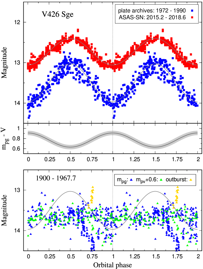
Figure 2: Top: Phase diagram for periodic wave-like variations in the ASASSN $V$ and $m_{\rm pg}$ LCs of V426 Sge according to the ephemeris (1). Grey lines represent their sinusoidal fits. Middle: Corresponding colour index $m_{\rm pg}-V$ illustrated by the black line inside the grey belt (= its uncertainty) (Sect. 3.1.2). Bottom: Photographic magnitudes prior to the 1968 outburst phased with the ephemeris (1). The LCs do not show any sinusoidal light variation along the orbit (Sect. 4.3.1).

Figure 3: Broadening of He ii $\lambda$4686, H$\beta$ and H$\alpha$ line profiles during the outburst (magenta, spectrum 2018/08/13.814 in Table 7) with respect to quiescent phase (blue, spectrum 2019/11/13.760 in Table 7). Local continuum is subtracted.

3.2 Physical parameters during the 2018 outburst

In this section we determine physical parameters of V426 Sge and describe their temporal evolution throughout the 2018 outburst. Our analysis is similar to the one we used for the 2015 outburst of AG Peg, because of their close similarity (see Skopal et al. 2017, and Sect. 4.1 here). Therefore, our approach is explained here only briefly.

3.2.1 Parameters from SED models

Modelling the near-UV (NUV) to NIR continuum allows us to determine parameters of the main components of radiation contributing to the observed spectrum. In the given spectral domain, we consider radiation emitted by the giant hot component ($\equiv$ the WD pseudophotosphere) and nebula. Using the method of disentangling the composite continuum of symbiotic binaries (see Skopal 2005a), we can determine the effective temperature of the giant, $T_{\rm eff}$, its radius, $R_{\rm G}$, the electron temperature of the nebula, $T_{\rm e}$, and its emission measure, EM. The luminosity of the WD pseudophotosphere, $L_{\rm WD}$, and its effective radius, $R_{\rm WD}^{\rm eff}$ (i.e. the radius of a sphere with the same luminosity), can be obtained for independently determined temperature, $T_{\rm WD}$ (Sect. 3.2.2). We selected the model corresponding to a minimum of the reduced $\chi^{2}$ function as the best model of our SED-fitting analysis. Owing to systematic errors in the calibration of some parts of our spectra, we adopted relatively large uncertainties of 10% for selected continuum fluxes in all our low-resolution spectra. Therefore, models of well-calibrated spectra are characterised with $\chi_{\rm red}^{2}<1$ (Table 8). More details can be found in Skopal et al. (2017). Modelling observations within different spectral domains requires a specific approach:

(i) In the case of fitting just the optical continuum, the method only makes it possible to disentangle contributions from the nebula and the cool giant, because of a very small contribution from the hot WD pseudophotosphere in the optical (see Sect. 3.2.2). Therefore, here we only determined parameters, $T_{\rm e}$, EM, $R_{\rm G}$, and $T_{\rm eff}$, where $T_{\rm eff}$ corresponds to the spectral type (ST) of the giant according to the calibration of Fluks et al. (1994). The ST subclass was estimated by a linear interpolation of two neighbouring best-fitting STs.

(ii) In modelling the Swift-UVOT/optical continuum we first fitted its optical part following the method (i) above. We then added a blackbody radiation for $T_{\rm WD}$ interpolated to dates of Swift-UVOT observations (see Table 9) and tuned all other variables to obtain an appropriate SED model. In this way we estimated the parameters $R_{\rm WD}^{\rm eff}$, $T_{\rm e}$, EM, $R_{\rm G}$, $T_{\rm eff}$, and $L_{\rm WD}$ from the Stefan-Boltzman law. In addition, the extreme sensitivity of mainly the UVM2 flux ($\lambda$ = 2246 Å) to the interstellar attenuation by dust and a strong dependence of both the height of the Balmer jump and the profile of the nebular continuum in the NUV on $T_{\rm e}$ allow us to verify the light reddening. This is because the lower values of the UV fluxes require a lower $T_{\rm e}$, which produces a higher Balmer jump, and vice versa. Accordingly, modelling the observations from October 6 and 7, 2018, when fluxes in all Swift-UVOT filters are available and the Balmer jump is well defined, allowed us to specify the colour excess $E_{\rm B-V}$ to 0.2$\pm 0.02$ mag. The corresponding upper and lower limits of the Swift-UVOT fluxes are shown in the panel (3,1) of Fig 4.

(iii) In modelling the optical/NIR continuum fluxes, we first fitted the optical part of the SED as in point (i), because the models of Fluks et al. (1994) are calculated only for $\lambda<10\,000$ Å. The optical SED was then connected with a synthetic spectrum of the same ST selected from a grid of models made by Hauschildt et al. (1999) so as to match the $JHKL$ fluxes. Here, we obtained the same fitting parameters as in (i), but the well-determined bolometric flux of the giant provided trustworthy fundamental parameters, that is, $L_{\rm G}$, $R_{\rm G}$, and $T_{\rm eff}$ (see Sect. 3.6, Fig. 10).

Table 8: Parameters from SED models: ST of the M giant, $T_{\rm e}$, $EM$, and a minimum of the $\chi_{\rm red}^{2}$ function (see Sect. 3.2.1).

Date	ST	$T_{\rm e}$	$EM$	$\chi_{\rm red}^{2}$/d.o.f.
yyyy/mm/dd.ddd		(K)	(1060 cm-3)
2018 outburst
2018/08/10.851	3.4	45000	6.61	0.47/1359
2018/08/10.905a	3.3	40000	7.29	0.48/982
2018/08/11.944b	2.5	43000	7.34	1.11/1330
2018/08/15.888	2.8	30000	6.54	0.34/935
2018/08/18.896	2.7	30000	6.86	0.43/849
2018/08/19.895	3.2	29500	5.22	0.63/1186
2018/08/21.899	2.6	24000	4.24	0.80/1557
2018/08/28.860c	3.5	21000	3.19	1.51/1954
2018/09/01.828	3.5	21000	2.93	1.04/1614
2018/09/07.886	3.3	20000	2.78	0.72/894
2018/09/11.903d	3.5	21000	2.74	0.65/1283
2018/09/15.911	3.7	19500	2.57	0.67/867
2018/09/20.888	3.7	22000	2.27	0.76/1279
2018/09/21.318e	4.3	19000	2.39	1.57/5607
2018/09/28.911	4.2	20000	2.42	0.78/910
2018/10/07.712f	3.3	16000	1.55	1.60/1628
2018/10/17.732	3.7	17600	1.50	0.67/1554
2018/11/18.708	4.9	19500	1.14	0.93/1388
2018/12/08.681	4.8	22000	1.08	1.37/1440
2018/12/17.704	4.5	14000	0.60	0.80/1330
Quiescent phase
2019/03/03.179	4.8g	18000h	0.26	i
2019/06/23.872	4.8	15000h	0.18	i
2019/08/19.832	4.6	45000	0.28	0.83/1418
2019/09/07.191	4.8	30000h	0.45	0.76/1018
2019/10/05.112	4.6	40000h	0.72	0.39/ 935

Notes. ^(a) spectra in Table 6, 2018/08/10.878 and 2018/08/10.932, ^(b) 2018/08/11.915 and 2018/08/11.972, ^(c) UVW2, UVM2 from 2018/08/28.7 and spectrum 2018/08/28.860, ^(d) UVW2 from 2018/09/11.45 and spectrum 2018/09/11.903, ^(e) UVW2 from 2018/09/18.10 and spectra 2018/09/19.827 and 2018/09/22.808, ^(f) UVW2, UVM2, UVW1 from 2018/10/06.44 and spectrum 2018/10/07.712, ^(g) adapted value, ^(h) given by the $U$ flux-point, ⁽ⁱ⁾ a comparison only.

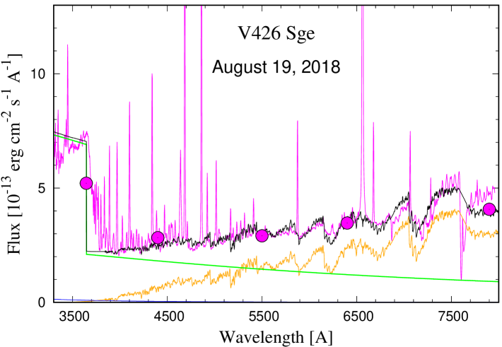
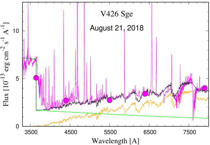
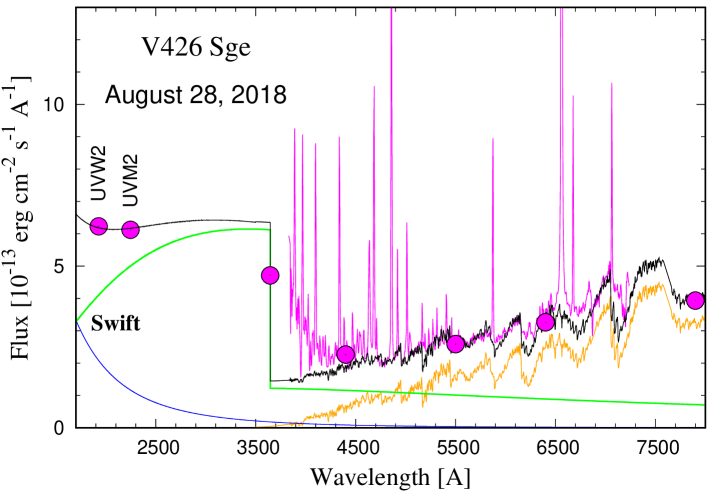
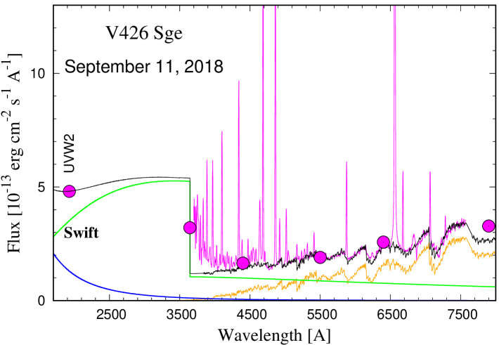
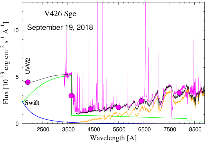
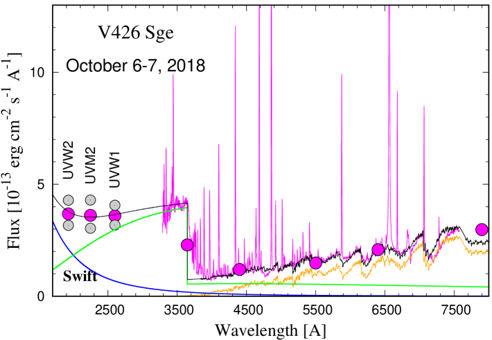
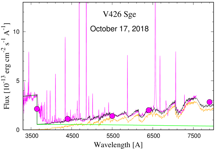
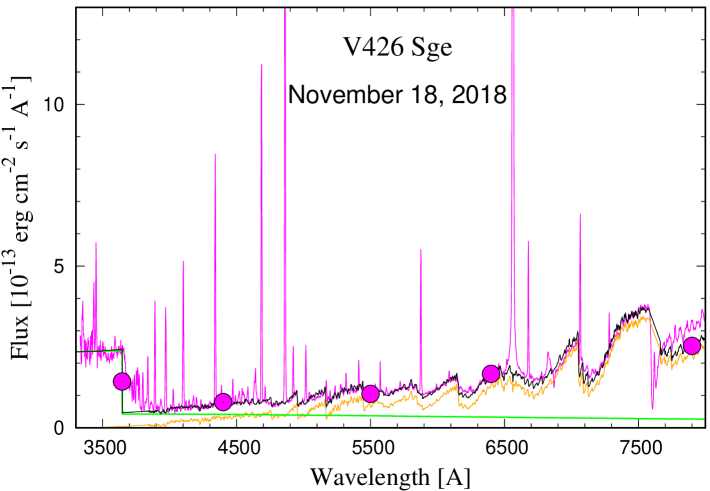
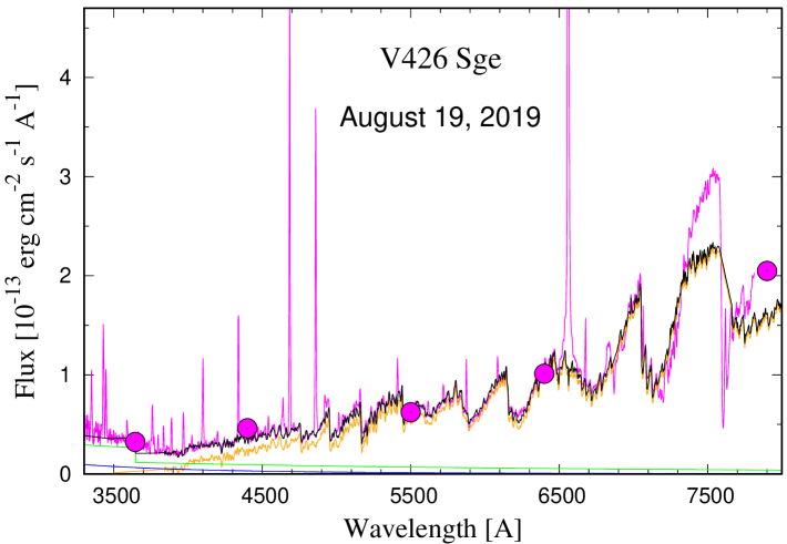
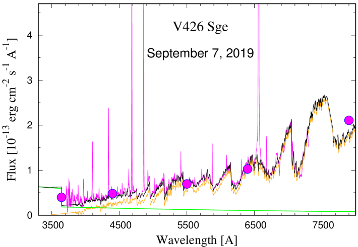
Figure 4: Examples of the observed (in magenta) and modelled (black lines) SEDs of V426 Sge at selected dates during its 2018 outburst and 2019 quiescent phase (bottom row). Lines and symbols are as shown in the keys (top left panel). Grey circles in the panel (3,1) are Swift-UVOT fluxes dereddened with the upper and lower limit of the $E_{\rm B-V}$ excess, 0.22 and 0.18 mag, respectively (see Sect. 3.2.1).

3.2.2 Temperature of the WD pseudophotosphere

According to the presence of strong He ii $\lambda$4686 and H$\beta$ emission lines in the spectrum of V426 Sge, we apply the He ii($\lambda 4686$)/H$\beta$ method to estimate the temperature of the WD pseudophotosphere, $T_{\rm WD}$. We introduce our approach as follows.

(i) The output energy via the He ii $\lambda$4686 transitions produced by the He⁺² zone is

$$4\pi d^{2}F_{\rm 4686}=\alpha_{4686}(T_{\rm e})h\nu_{4686}\,EM({\rm He}^{+2}),$$ (2)

where $F_{\rm 4686}$ is the observed line flux, $EM({\rm He}^{+2})=n_{\rm e}n({\rm He}^{+2})V$ is the emission measure of the He⁺² zone, $\alpha_{4686}(T_{\rm e})$ is the effective recombination coefficient for the transition, $n_{\rm e}$ and $n({\rm He}^{+2})$ are mean concentrations of electrons and He⁺² ions, and $V$ is the volume of the He⁺² zone.

(ii) The input energy for that given by Eq. (2) is represented by the flux of stellar photons capable of ionising He⁺ ions,

$$Q(4\nu_{0},\infty)=\alpha_{\rm B}({\rm He}^{+},T_{\rm e})EM({\rm He}^{+2}),$$ (3)

where $\nu_{0}$ is the ionising frequency of hydrogen and $\alpha_{\rm B}({\rm He}^{+},T_{\rm e})$ is the total recombination coefficient of He⁺ for Case B (i.e. the nebula is optically thick to ionising radiation). Accordingly, substituting $EM({\rm He}^{+2})$ from (3) to (2), we can write Eq. (2) in the form

$$4\pi d^{2}F_{\rm 4686}=\alpha_{4686}(T_{\rm e})h\nu_{4686}\,\frac{Q(4\nu_{0},\infty)}{\alpha_{\rm B}({\rm He}^{+},T_{\rm e})}.$$ (4)

Using the same approach for the H$\beta$ line created within the H⁺ zone, we can write the flux ratio (see also Gurzadyan 1997),

$$\frac{F_{4686}}{F_{{\rm H}\beta}}=\frac{\alpha_{4686}(T_{\rm e})}{\alpha({\rm H}\beta,T_{\rm e})}\,\frac{\alpha_{\rm B}({\rm H}^{0},T_{\rm e})}{\alpha_{\rm B}({\rm He}^{+},T_{\rm e})}\,\frac{\nu_{4686}}{\nu_{4861}}\,\frac{Q(4\nu_{0},\infty)}{Q(\nu_{0},4\nu_{0})},$$ (5)

where the flux of hydrogen ionising photons, $Q(\nu_{0},4\nu_{0})$, is calculated only between $\nu_{0}$ and $4\nu_{0}$, because recombinations of He⁺² to He⁺ within the innermost He⁺² zone ($\nu>4\nu_{0}$) produce sufficient quanta to keep the hydrogen ionised (see Hummer & Seaton 1964). The principle of this method was first suggested by Ambartsumyan (1932). The method was later elaborated by Harman & Seaton (1966) and further modified by other authors (e.g. Iijima 1981; Kaler & Jacoby 1989).

Optically thick conditions where the nebula is not transparent to ionising radiation are indicated by the presence of elements at very different ionisation states in the spectrum, such as during the outburst of AG Peg (see Skopal et al. 2017, and references therein) and the increase of particle density around the WD due to the increase of the mass-loss rate from the WD (see Sect. 3.2.4). Applying Eq. (5) to He ii($\lambda 4686$)/H$\beta$ flux ratios (Table 13), we used recombination coefficients from Hummer & Storey (1987) for $T_{\rm e}$ = 30 000 and 20 000 K for August 10 to 22 and August 27 to December 17, 2018, respectively (see Table 8), and for the electron concentration of $10^{10}$ cm^-3 (e.g. Skopal et al. 2011). Equation (5) can subsequently be expressed as

$$\frac{F_{4686}}{F_{{\rm H}\beta}}=\xi\,\frac{Q(4\nu_{0},\infty)}{Q(\nu_{0},4\nu_{0})},$$ (6)

where $\xi$ = 1.30 and 1.33 for $T_{\rm e}$ = 30 000 and 20 000 K, respectively. The number of quanta $Q$ was calculated for Planck’s function. Resulting $T_{\rm WD}$ are listed in Table 9 and plotted in Fig. 5. During the quiescent phase, the method is not applicable because the nebula is only partly ionisation-bounded, that is, a fraction of ionising photons escape the nebula without being converted to diffuse radiation.

Uncertainties in $T_{\rm WD}$ are around 5%. They are given by errors in the used He ii($\lambda 4686$) and H$\beta$ line fluxes (see Table 13), the values of which depend mostly on the determination of the true continuum. Here, the main sources of uncertainty are the noise in the local continuum and its calibration to photometric flux points.

3.2.3 Luminosity and radius of the ionising source

Having only the optical spectra, we can only indirectly estimate the luminosity $L_{\rm WD}$, under the assumption that the total flux of hydrogen ionising photons produced by the WD pseudophotosphere, $Q(\nu_{0},\infty)$, is balanced by the total rate of recombinations within the ionised volume, that is,

$$Q(\nu_{0},\infty)=\alpha_{\rm B}({\rm H^{0}},T_{\rm e})\,\textsl{EM},$$ (7)

where $\alpha_{\rm B}({\rm H^{0}},T_{\rm e})$ is the recombination coefficient to all but the ground state of hydrogen (i.e. Case $B$). Having the quantity of EM from SED models we can then estimate the corresponding $L_{\rm WD}$ for the given temperature of the ionising source, $T_{\rm WD}$ (Sect. 3.2.2), according to expression,

$$L_{\rm WD}=\alpha_{\rm B}({\rm H^{0}},T_{\rm e})\,\textsl{EM}\frac{\sigma T_{\rm WD}^{4}}{f(T_{\rm WD})},$$ (8)

where the function $f(T_{\rm WD})$ determines the flux of ionising photons emitted by the 1 cm² area of the ionising source (see Skopal et al. 2017, in detail). The effective radius of the WD pseudophotosphere, $R_{\rm WD}^{\rm eff}$, is then given by the Stefan-Boltzmann law.

Having $T_{\rm WD}$ from high-resolution spectra (Table 7) and EM from low-resolution spectra (Table 6) we interpolated EM values to dates of high-resolution spectra. Corresponding $L_{\rm WD}$ from Eq. (8) with other parameters are listed in Table 9 and their temporal evolution along the outburst is shown in Fig. 5 with filled symbols. We also interpolated $T_{\rm WD}$ values to dates of low-resolution spectra and plotted the corresponding parameters in Fig. 5 with open symbols. Parameters $L_{\rm WD}$ and $R_{\rm WD}^{\rm eff}$ determined directly from the radiation of the WD pseudophotosphere with the aid of modelling the Swift-UVOT/optical continuum (Sect. 3.2.1) are shown in Table 9. Their quantities are comparable to those obtained indirectly from the EM. However, their large scatter is a result of less accurate scaling and the temperature estimated from line ratios.

Table 9: Parameters of the WD pseudophotosphere, $L_{\rm WD}$ (10³⁷$\rm\,erg\,s^{-1}$), $R_{\rm WD}^{\rm eff}$ ( $R_{\sun}$), $T_{\rm WD}$ (10⁵ K) and $\dot{M}_{\rm WD}$ (10^-6 $M_{\sun}\,{\rm yr}^{-1}$) along the 2018 outburst of V426 Sge (see Sects. 3.2.2, 3.2.3 and 3.2.4).

Date	$L_{\rm WD}$	$R_{\rm WD}^{\rm eff}$	$T_{\rm WD}$	$\dot{M}_{\rm WD}$
2018/08/10.845	6.8$\pm$0.7	0.070$\pm$0.004	2.53$\pm$0.13	2.36
2018/08/11.826	7.3$\pm$0.8	0.079$\pm$0.005	2.41$\pm$0.12	2.67
2018/08/13.814	6.0$\pm$0.7	0.101$\pm$0.006	2.03$\pm$0.12	3.00
2018/08/13.827	6.5$\pm$0.7	0.087$\pm$0.006	2.23$\pm$0.12	2.75
2018/08/15.853	6.7$\pm$0.7	0.071$\pm$0.005	2.49$\pm$0.13	2.37
2018/08/17.070	6.5$\pm$0.7	0.077$\pm$0.005	2.37$\pm$0.13	2.50
2018/08/17.896	5.8$\pm$0.7	0.099$\pm$0.006	2.03$\pm$0.12	2.92
2018/08/18.823	6.2$\pm$0.7	0.091$\pm$0.006	2.15$\pm$0.12	2.80
2018/08/19.842	4.8$\pm$0.6	0.079$\pm$0.006	2.18$\pm$0.12	2.27
2018/08/20.869	5.6$\pm$0.6	0.118$\pm$0.007	1.85$\pm$0.11	2.71
2018/08/22.840	4.8$\pm$0.6	0.114$\pm$0.007	1.81$\pm$0.11	2.47
2018/08/27.796	3.9$\pm$0.5	0.107$\pm$0.006	1.77$\pm$0.10	2.15
2018/09/07.867	3.0$\pm$0.5	0.111$\pm$0.006	1.63$\pm$0.09	2.00
2018/09/19.821	2.6$\pm$0.4	0.099$\pm$0.006	1.66$\pm$0.09	1.71
2018/09/20.837	2.4$\pm$0.4	0.108$\pm$0.006	1.56$\pm$0.08	1.78
2018/10/04.840	1.9$\pm$0.4	0.103$\pm$0.006	1.50$\pm$0.09	1.56
2018/10/05.724	1.9$\pm$0.4	0.085$\pm$0.006	1.67$\pm$0.09	1.36
2018/10/10.788	1.7$\pm$0.3	0.075$\pm$0.005	1.73$\pm$0.10	1.18
2018/10/11.835	1.6$\pm$0.4	0.086$\pm$0.006	1.59$\pm$0.09	1.28
2018/10/16.713	1.6$\pm$0.3	0.091$\pm$0.006	1.53$\pm$0.07	1.31
2018/10/18.797	1.7$\pm$0.3	0.067$\pm$0.005	1.84$\pm$0.11	1.09
2018/10/20.757	1.7$\pm$0.3	0.072$\pm$0.005	1.75$\pm$0.10	1.13
2018/11/10.773	1.4$\pm$0.3	0.062$\pm$0.005	1.82$\pm$0.10	0.95
2018/11/12.803	1.3$\pm$0.2	0.074$\pm$0.004	1.62$\pm$0.09	1.04
2018/11/23.729	1.3$\pm$0.2	0.063$\pm$0.004	1.75$\pm$0.10	0.91
2018/12/17.701	0.7$\pm$0.1	0.043$\pm$0.003	1.82$\pm$0.11	0.52
From Swift-UVOT/optical SED models
2018/08/28.722	5.4$\pm$0.6	0.128$\pm$0.008	1.76a	–
2018/09/11.451	2.9$\pm$0.4	0.107$\pm$0.007	1.64a	–
2018/09/18.101	3.4$\pm$0.5	0.116$\pm$0.007	1.65a	–
2018/10/06.440	4.7$\pm$0.6	0.133$\pm$0.008	1.67a	–
2019/03/03.179	0.89$\pm$0.13	0.071$\pm$0.005	1.50b	–

Notes. ^(a) Interpolated value to dates of Swift-UVOT observations, ^(b) adopted value

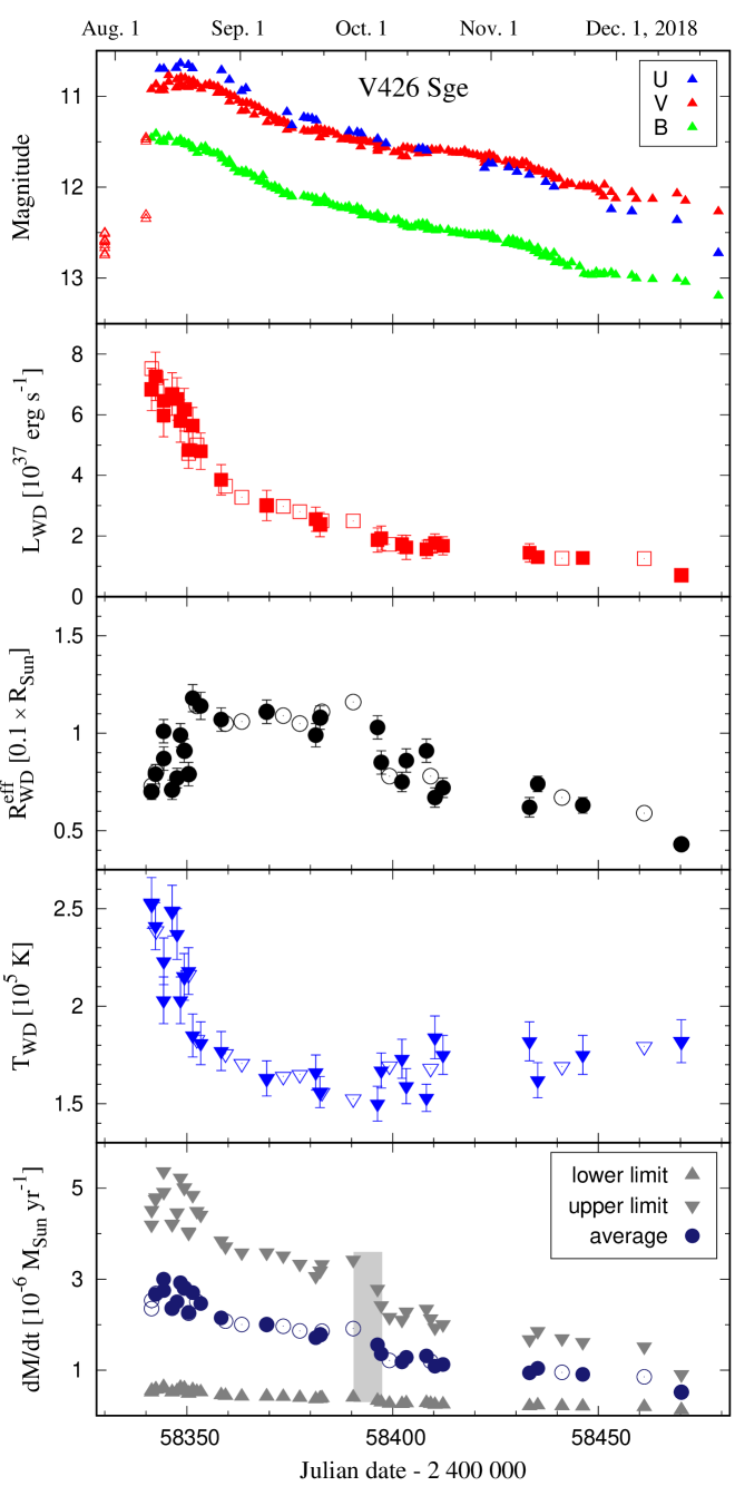
Figure 5: Evolution of the parameters $L_{\rm WD}$, $R_{\rm WD}^{\rm eff}$, $T_{\rm WD}$ and $\dot{M}_{\rm WD}$ throughout the 2018 outburst of V426 Sge (data from Table 9). The meaning of filled and open symbols is explained in Sect. 3.2.3. The grey belt in the bottom panel denotes the time of a drop in $\dot{M}_{\rm WD}$ (see Sect. 4.2).

3.2.4 Mass-loss rate from the burning WD

A strong nebular emission with EM of a few times 10⁶⁰ cm^-3 develops during active phases of symbiotic stars (Skopal 2005a). It is produced by the ionised wind from the burning WD, the emissivity of which is given by the mass-loss rate (Skopal 2006). Therefore, having EM from SED models and adopting an appropriate model for the stellar wind, we can determine the corresponding mass-loss rate, $\dot{M}_{\rm WD}$.

As in the case of AG Peg, we consider the $\beta$-law wind according to Lamers & Cassinelli (1999). The wind begins at the radial distance from the WD centre $r=R_{0}$ with the initial velocity $a$ and becomes optically thin at $r=R_{\rm in}$. Further, the velocity profile of the wind is characterised by the acceleration factor $\beta$ and the terminal velocity $v_{\infty}$. Assuming a spherically symmetric wind around the WD, we can express a relationship between EM and $\dot{M}_{\rm WD}$ of the ionised wind as (Skopal et al. 2017),

$$\textsl{EM}=\xi\,\Big{(}\frac{\dot{M}_{\rm WD}}{v_{\infty}}\Big{)}^{2}\frac{1}{bR_{0}(1-2\beta)}\Big{[}1-\Big{(}1-\frac{bR_{0}}{R_{\rm in}}\Big{)}^{1-2\beta}\Big{]}\leavevmode\nobreak\ ,$$ (9)

where $\xi=1.45\times 10^{46}$ g^-1 and the parameter $b=1-(a/v_{\infty})^{1/\beta}$. Using Eq. (9) we determined $\dot{M}_{\rm WD}$ for EM (Table 8), $v_{\infty}=2000$ km s^-1 (from H$\alpha$ wings, Fig. 3), $\beta\sim 1.7$, $a$ = 50 km s^-1 and assuming $R_{\rm in}=R_{\rm WD}^{\rm eff}$ (see Sect. 3.2.6. of Skopal et al. 2017, and references therein). Because a significant fraction of the wind emission is produced within its densest innermost part, the corresponding $\dot{M}_{\rm WD}$ strongly depends on the wind origin, $R_{\rm 0}$, which, however, cannot be derived from observations. Therefore, according to the theory of the optically thick wind in nova outbursts (e.g. Kato & Hachisu 1994), we consider two limiting values of $R_{\rm 0}$ within the shell around the WD:

1. $R_{\rm 0}=R_{\rm WD}^{\rm eff}$, which corresponds to the lower limit of $\dot{M}_{\rm WD}$. Our values of EM and $R_{\rm WD}^{\rm eff}$ imply $\dot{M}_{\rm WD}=2-5\times 10^{-7}$ $M_{\sun}\,{\rm yr}^{-1}$.

2. $R_{\rm 0}=R_{\rm WD}$, which provides the upper limit of $\dot{M}_{\rm WD}$. Our measurements and $R_{\rm WD}\equiv 0.01$ $R_{\sun}$ correspond to $\dot{M}_{\rm WD}=1-5\times 10^{-6}$ $M_{\sun}\,{\rm yr}^{-1}$.

Table 9 presents the average of these limiting values that are between $\sim$1 and $\sim$3$\times 10^{-6}$ $M_{\sun}\,{\rm yr}^{-1}$, while Fig. 5 shows all quantities of $\dot{M}_{\rm WD}$.

3.3 Raman-scattered O vi lines

The evolution of the Raman-scattered O vi 6825 Å line profile and its flux along the outburst of V426 Sge are very similar to those observed during the 2015 outburst of AG Peg (see Figs. 5 and 9 of Skopal et al. 2017, and Figs. 6 and 8 here). Around the optical maximum, during August 10-12, 2018, the Raman line was not detectable, and hardly recognisable until August 19. From August 20, the Raman line was clearly seen above the continuum showing two emission bumps in its profile at $\sim$6827 and $\sim$6838 Å. Both components were comparable in the profile and flux until about September 7. The blueshifted component then became stronger and broader being located around the Raman transition at 6825.44 Å during the whole active phase. The redshifted component was stable at its position with no significant variation in the profile and flux (see Fig. 6). Finally, it is of interest to note that maximum fluxes of the Raman line observed during the 2015 outburst of AG Peg ($\sim$5$\times 10^{-11}$$\rm\,erg\,s^{-1}\,cm^{-2}$) and during the 2018 outburst of V426 Sge ($\sim$2.2$\times 10^{-12}$$\rm\,erg\,s^{-1}\,cm^{-2}$) correspond to similar luminosities of $\sim$3.8$\times 10^{33}\,(d/0.8\,{\rm kpc})^{2}$$\rm\,erg\,s^{-1}$ and $\sim$2.9$\times 10^{33}\,(d/3.3\,{\rm kpc})^{2}$$\rm\,erg\,s^{-1}$ for AG Peg and V426 Sge, respectively. During the following quiescent phase, our only high-resolution spectrum from November 2019 indicates a similar profile to that from the end of the outburst, but fainter by a factor of about 0.5 (Fig. 6, Table 13). Similar evolution of the Raman line profile and flux during recent outbursts of AG Peg and V426 Sge suggests that their ionisation structure was similar (see Sect. 4.1).

In regards to the Raman O vi 7082 Å line, its profile was difficult to indicate in the spectrum. If we can associate the small emission at $\sim$+20 km s^-1 to the O vi 7082 Å line (see Fig. 7), then the flux ratio $F(6825)/F(7082)$ is between 10 and 30, which is anomalously high. For the ratio of the parent O vi lines $F(1032)/F(1038)\sim 1$, Lee et al. (2016) found the flux ratio $F(6825)/F(7082)$ to be between 1 and 3, depending on the H⁰ column density. However, in some cases we observe this ratio to be around 6 (Birriel et al. 2000) and probably even larger for AG Peg (see Fig. 10 of Skopal et al. 2017). A very high ratio in the range of $F(1032)/F(1038)\sim 7-20$ was reported by Birriel et al. (1998) and Schmid et al. (1999), who explained this anomaly by a significant attenuation of the O vi 1038 Å line by the interstellar H₂ absorption. If we can assume the presence of the H₂ molecules also within the circumstellar H⁰ region, then H⁰ column densities of 10^23-24 cm^-2 with the abundance of H/H${}_{2}=10^{2-3}$ give a flux ratio of $F(6825)/F(7082)=10-20$ or more (see Fig. 8 of Schmid et al. 1999). However, this suggestion requires theoretical verification, which is beyond the scope of this paper.

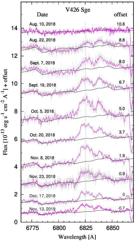
Figure 6: Evolution of the Raman-scattered O vi 6825 Å line along the 2018 outburst of V426 Sge. The grey and magenta lines show original and smoothed spectra, respectively, the vertical dotted line represents the wavelength of the Raman transition at 6825.44 Å, the black lines represent the continuum, and the numbers on the right mark the spectra offset.

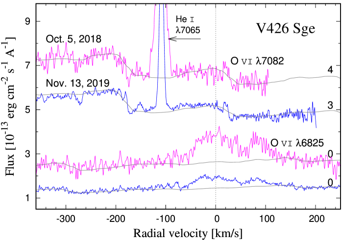
Figure 7: Example of the Raman scattered O vi 7082 and 6825 Å lines measured during the outburst (in magenta) and quiescence (in blue). Other denotations as in Fig. 6.

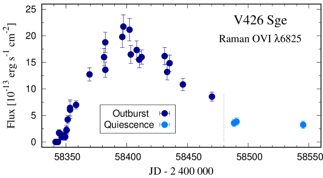
Figure 8: Fluxes of the Raman-scattered O vi 6825 Å line during the outburst (dark blue) and following quiescence (light blue). Values from quiescence were shifted by -170 days for better comparison.

3.4 Swift-XRT emission from colliding winds

The X-ray emission from V426 Sge during its 2018 outburst is very soft, as more than 92% of X-ray photons are detected below 2 keV (Sect. 2.1.1). On the other hand, the super-soft X-rays from a $\sim$180 kK hot WD pseudophotosphere producing a luminosity of $\sim 3\times 10^{-8}$$\rm\,erg\,s^{-1}\,cm^{-2}$ at the Earth (see values in Table 9 after August 28, 2018 – the first XRT observations) cannot be detected within the Swift-XRT energy range (see Fig. 13 of Skopal 2019, for a comparison). Such a location of the X-ray emission from V426 Sge is most consistent with the so-called $\beta$-type (see Mürset et al. 1997; Luna et al. 2013). In addition, the X-ray fluxes correspond to luminosities of a few times $10^{32}\,(d/3.3\,{\rm kpc})^{2}$$\rm\,erg\,s^{-1}$ (Table 1) which are typical for symbiotic binaries producing this type of X-ray (see Table 2 of Mukai 2017). According to Mürset et al. (1995), this type of X-ray spectrum can be reproduced by shock-heated plasma as a result of colliding winds. Also, Mukai (2017) connected these X-ray properties with the energy source resulting from colliding winds in symbiotic binaries.

The same origin of the Swift-XRT emission from the outburst of V426 Sge is strongly supported by the enhanced wind from the WD (Fig. 5). According to the ionisation structure during the outburst (Sect. 4.1), a biconical wind from the WD can collide with the wind from the cool giant in the interaction zone well above the orbital plane and at distances greater than the size of the binary (e.g. Fig. 4 of Mürset et al. 1995). Therefore, such emission is well observable as it is only slightly attenuated by the interstellar absorption corresponding to $E_{\rm B-V}=0.2$ mag.

Accordingly, during the quiescent phase, the indication of the X-ray emission was negative (Table 1, Swift-XRT pointing on March 3, 2019), because the wind from the WD terminated (see Sect. 3.5).

3.5 Transition to quiescent phase

The optical brightening during the outburst was governed exclusively by the nebular component of radiation, whose contribution dominates the $U$ band (Fig. 4). Therefore, the $U$ magnitude is also proportional to $\dot{M}_{\rm WD}$ during the outburst, because $EM\propto(\dot{M}_{\rm WD})^{1/2}$ (Eq. (9)). As a result, a rapid decline in the brightness of the star in $U$ from December 5-7, 2018, to February 15, 2019 (see Fig. 9), reflects a rapid decrease in $\dot{M}_{\rm WD}$. After this period, $UBV$ colour indices came to a constant state and the LCs indicated development of the wave-like orbitally related variation, a typical feature of the quiescent phase (see panels c and d of Figs. 1 and 9). This means that the wind from the WD, and thus the outburst, ceased around the middle of February, 2019, and V426 Sge moved into a quiescent phase. A new source of a relative faint nebular emission ($EM\sim 2-7\times 10^{59}$ cm^-3, Table 8) is now represented by the ionised fraction of the wind from the giant (Sect. 1).

3.6 Parameters of the red giant

To obtain parameters of the red giant in V426 Sge, we modelled two SEDs determined by the optical spectrum and $UBVR_{\rm C}I_{\rm C}JHKL$ photometry, observed almost simultaneously during quiescent phase on June 22 and 23 and August 19 and 24, 2019 (see Tables 3 and 6 for precise timing). Observations and models are depicted in Fig. 10.

Fitting the optical spectrum, we determined the ST of the giant as M4.7($\pm$0.2) III which corresponds to $T_{\rm eff}\sim 3\,400$ K according to the calibration of Fluks et al. (1994). We then matched both the optical and the NIR fluxes by a synthetic spectrum calculated for $T_{\rm eff}=3\,400$ K. The model corresponds to the observed bolometric flux $F_{\rm G}^{\rm obs}=3.85$ and $4.15\times 10^{-9}$$\rm\,erg\,s^{-1}\,cm^{-2}$ and the angular radius of the giant, $\theta_{\rm G}=7.2$ and $7.4\times 10^{-10}$ (see Eqs. (3) and (4) of Skopal 2005a), for the model from June and August, 2019, respectively. Our values of $\theta_{\rm G}$ are in good agreement with those derived from the surface brightness relation for M-giants (see Dumm & Schild 1998), $\theta_{\rm G}=7.3$ and $7.6\times 10^{-10}$, given by the reddening-free magnitudes $J=7.77$, $K=6.62$, and $J=7.67$, $K=6.52$ for the two SED models above, respectively. Finally, our values of $\theta_{\rm G}$ give the radius $R_{\rm G}=104$ and $108\,(d/3.3\,\,{\rm kpc})$ $R_{\sun}$ and the luminosity $L_{\rm G}=1\,300$ and $1400\,(d/3.3\,\,{\rm kpc})^{2}$ $L_{\sun}$ for the first and second model SED, respectively. Uncertainties for such determined parameters are of $\sim$5% only, but for fixed $T_{\rm eff}$.

Variability in the giant is suggested by the large scatter in the model ST (M2.5 – M4.9 III, see Table 8) and in its scaling $\theta_{\rm G}$ (see Fig. 4). It is of interest to note that the earlier ST is limited to the early outburst evolution, while the changes in the angular radius seem to be random, probably connected with the intrinsic variability of the giant. The former effect was observed also during the 2015 outburst of AG Peg (see Table 4 of Skopal et al. 2017) and during the 2015 super-active state of recurrent nova T CrB (Munari et al. 2016). This effect requires further investigation, which is beyond the scope of this paper.

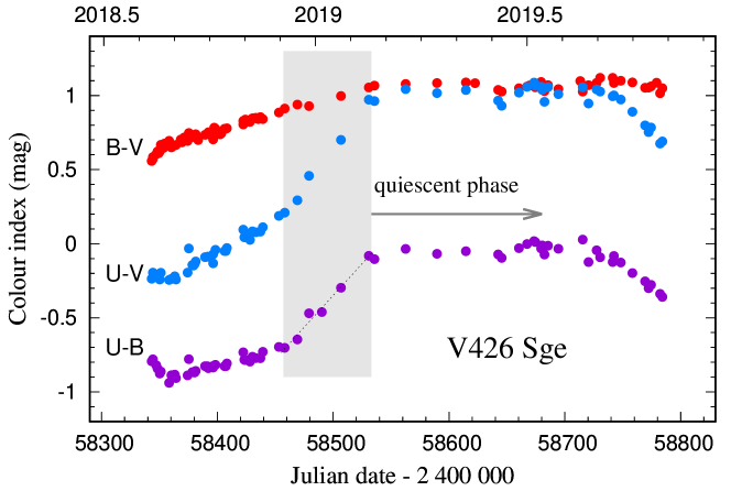
Figure 9: Transition of V426 Sge from its 2018 outburst to quiescent phase as indicated by our $UBV$ photometry (Table 10). The grey belt indicates a rapid decrease of $\dot{M}_{\rm WD}$ to around the middle of February 2019, when V426 Sge moved to quiescent phase (see Sect. 3.5).

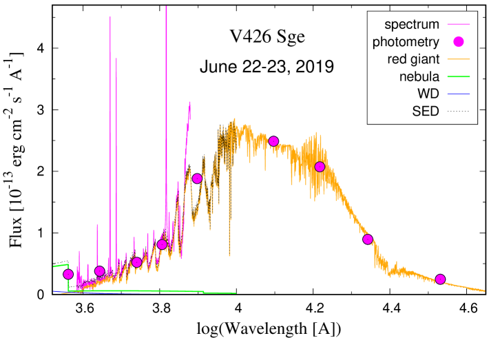
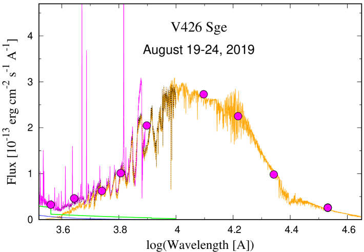
Figure 10: Optical/NIR SED of V426 Sge during quiescent phase. The observed SED (low-resolution spectrum and $UBVR_{\rm C}I_{\rm C}JHKL$ photometry) is matched by a synthetic spectrum, corresponding to spectral type M4.8 (top) and M4.6 (bottom) or $T_{\rm eff}\sim 3400$ K (see Sect. 3.6).

4 Discussion

4.1 Comparison with AG Peg

The SED models during the 2015 and 2018 outburst of AG Peg and V426 Sge are essentially the same: a strong nebular component of radiation, which is responsible for the optical brightening, a more or less constant contribution from the cool giant, and a very hot stellar component from the WD whose contribution is negligible in the optical (see Fig. 4 of Skopal et al. 2017, and Fig. 4 here). Thus, the brightness increase and its evolution along both the outbursts have the same origin: injection of particles into the particle-bounded nebula around the WD, which as a result becomes ionisation-bounded. This change leads to production of an extra nebular emission due to the increase of the rate of recombinations that balance the increased flux of ionising photons. Under the optically thick conditions we can then derive fundamental parameters of the source of the original stellar radiation (which is the WD pseudophotosphere) from its fraction converted to the nebular radiation (see Sects. 3.2.2 and 3.2.3). In both cases, we derived a more than one order of magnitude increase in the EM relative to values from the quiescent phase, which corresponds to a mass-loss rate from the WD of a few times 10^-6 $M_{\sun}\,{\rm yr}^{-1}$ (see Sect. 3.2.4).

Both stars show also the same type of the X-ray emission during their recent outbursts. The spectrum is of $\beta$-type, concentrated below 2 keV and with a luminosity of a few times $10^{32}$$\rm\,erg\,s^{-1}$ (see Ramsay et al. 2016, for AG Peg and Sect. 3.4 for V426 Sge).

The similar quantities found for the parameters $L_{\rm WD}$, $R_{\rm WD}^{\rm eff}$, and $T_{\rm WD}$ of the WD pseudophotosphere during the 2015 outburst of AG Peg and the 2018 outburst of V426 Sge (see Fig. 7 of Skopal et al. 2017, and Fig. 5 here) suggest that these outbursts are of the same nature. The high value of $L_{\rm WD}\sim 6\times 10^{37}$$\rm\,erg\,s^{-1}$ observed around the maximum of the 2018 outburst can only be generated by nuclear hydrogen burning on the surface of the WD. The corresponding accretion rate of $\sim 2\times 10^{-7}$ $M_{\sun}\,{\rm yr}^{-1}$ exceeds the upper limit of the stable-burning regime for a low-mass WD (see e.g. Shen & Bildsten 2007), which leads to the production of optically thick wind (see e.g. Hachisu et al. 1996) whose particles convert the ionising photons to the nebular emission that dominates the NUV/optical domain; we observe the Z And-type outburst of the 2nd-type (i.e. the ‘hot-type’ outburst; see Sect. 4.2).

Also during quiescent phase, fundamental parameters of the burning WD are comparable for both stars (here, Table 9, the Swift-UVOT/optical SED model on March 3, 2019). The luminosity of $\sim$2300 $L_{\sun}$ emitted by the WD photosphere at a high temperature of $\approx$150 kK corresponds to a $\sim$0.5 $M_{\sun}$ WD that burns hydrogen on its surface at the rate of its accretion (see e.g. Fig. 1 of Nomoto et al. 2007). Thus, both symbiotic binaries also harbour a low-mass WD (see Kenyon et al. 1993, for AG Peg).

Finally, a striking similarity in the evolution of the Raman-scattered O vi 6825 Å line profile and the increase of its flux during the recent outbursts of AG Peg and V426 Sge (see Sect. 3.3) suggest similar ionisation structure in these two systems: the presence of a neutral disc-like zone at the equatorial plane expanding from the WD and the ionised region located above and below the disc (see Fig. 12 and Sect. 4.7.3. of Skopal et al. 2017, and references therein). Accordingly, (i) the significant increase of the Raman line flux during both outbursts could be caused by an increase of the Raman scattering efficiency, because a larger fraction of the O⁺⁵ sky is covered by the neutral hydrogen during outbursts than in quiescence. During outbursts, the initial O⁺⁵ photons arising around the WD are located just above and below the scattering region (= the neutral disc), and can therefore ‘see’ the scattering region under a large solid angle, while during quiescence the H i zone around the giant (= the neutral fraction of the giant’s wind) is located far from the O⁺⁵ zone, and thus occupies a much smaller fraction of the O⁺⁵ sky. (ii) Broadening of the Raman line and development of a strong redshifted component at $\sim$6838 Å during outbursts can arise from such a disc-like zone of scatterers expanding from the source of the initial O⁺⁵ photons. This interpretation is independently supported by the presence of the Raman-scattered O vi lines in the spectrum of the luminous B[e] star LHA 115-S 18, where the Raman emission arises from a dense circumstellar disc of neutral hydrogen illuminated by the radiation from the central hot star (see Torres et al. 2012).

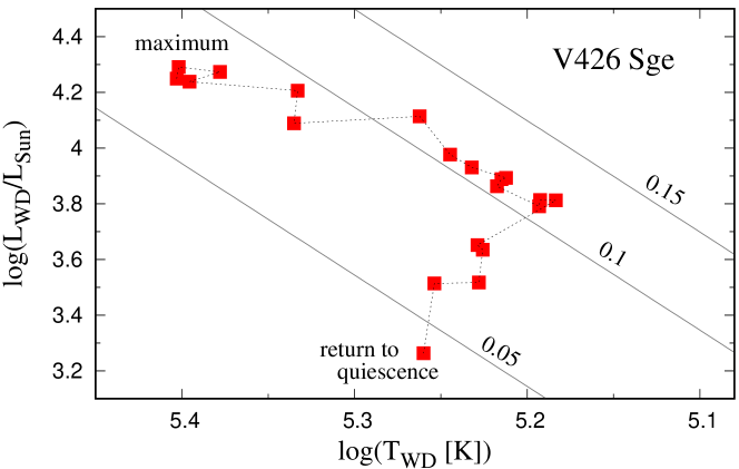
Figure 11: H-R diagram for the 2018 outburst of V426 Sge from around its optical maximum to the return to quiescence as given by our ground-based observations (Table 9). The dotted line follows the temporal evolution of the given parameters. Full lines represent loci with constant effective radii. Labels are in solar units (see Sect. 4.2).

4.2 The outburst in the H-R diagram

Figure 11 shows the evolution of the WD parameters, $L_{\rm WD}$, $R_{\rm WD}^{\rm eff}$, and $T_{\rm WD}$ in the H-R diagram from around the maximum of the outburst on August 10, 2018, to almost its end on December 17, 2018 (see Sects. 3.1.3 and 3.5 for the outburst timing and Table 9 for parameters). The highest values of $L_{\rm WD}$ and $T_{\rm WD}$ were measured around the maximum of the outburst, while the lowest $L_{\rm WD}$ and $R_{\rm WD}^{\rm eff}$ were observed close to its end. The most interesting feature in the diagram is the ‘knee’, when the effective radius starts to shrink more rapidly with a small increase of $T_{\rm WD}$ and a gradual decline of $L_{\rm WD}$. This change happened between September 28 and October 7, when $\dot{M}_{\rm WD}$ dropped by a factor of $\sim$1.5, from $\sim 2\times 10^{-6}$ to $\sim 1.3\times 10^{-6}$ $M_{\sun}\,{\rm yr}^{-1}$ (see grey vertical band in the bottom panel of Fig. 5). The following gradual decrease in $\dot{M}_{\rm WD}$ caused a relevant shrinkage of the optically thick/thin interface of the wind, i.e., the WD’s pseudophotosphere.

The position of fundamental parameters in the H-R diagram and the model SED suggest that the 2018 outburst of V426 Sge is of the 2nd-type; see Sect. 1. These outbursts are characterised by the immediate occurrence of a strong nebular emission and of a hot ($\approx 2\times 10^{5}$ K) ionising source from the very beginning of the outburst. Therefore, it is suitable to refer to these outbursts as ‘hot-type’ outbursts. On the other hand, it is appropriate to refer to the 1st-type outbursts as ‘warm-type’, because they are characterised by a warm (1–2$\times 10^{4}$ K) pseudophotosphere dominating the optical during outburst. According to Skopal (2005a), this classification implies that the V426 Sge binary has a low orbital inclination, which allows us to directly see the hot WD and its product during outbursts, that is, the ionised high-velocity wind as indicated by a remarkable increase of EM. Similar, well-observed systems showing hot-type outbursts are: AG Dra (e.g. Mikołajewska et al. 1995; Greiner et al. 1997; Skopal et al. 2009; Sion et al. 2012), AG Peg (e.g. Ramsay et al. 2016; Skopal et al. 2017; Sion et al. 2019), and LT Del (see Arkhipova et al. 1995; Ikonnikova et al. 2019).

4.3 The path to Z And-type outbursts

4.3.1 Observational constraints

Figure 12 shows development of the wave-like orbitally related variation in the LCs of symbiotic novae AG Peg, V1329 Cyg, and V426 Sge during the transition from their symbiotic nova outburst to quiescent phase. This type of the variability also developed in the LC of RT Ser after its symbiotic nova outburst in 1909 (see Shugarov et al. 2003) and in the LC of the symbiotic nova PU Vul during its return from the nova outburst in 1979 to quiescence (see Cúneo et al. 2018).

After around 20 and 28 years of quiescence, when the star’s brightness varied around a constant level, AG Peg and V426 Sge underwent an Z And-type outburst and became classical symbiotic stars (see Tomov et al. 2016; Ramsay et al. 2016; Skopal et al. 2017, for AG Peg and this paper for V426 Sge). For V1329 Cyg and V426 Sge, there is around 70 years of photometric observations prior to their symbiotic nova outbursts. In both cases, the pre-outburst LC does not show the sinusoidal light variation along the orbit or any direct evidence of symbiotic-like activity; some activity of this kind was recorded, but only approximately 5-7 years before the nova outburst. In the case of V1329 Cyg, oscillations within $\sim$0.8 mag with a gradual increase by $\sim$1 mag were indicated, while for V426 Sge, three $\sim$1 mag brightness decreases were measured, but these were out of the phase with the post-outburst variation (see Figs. 1, 2 and 12).

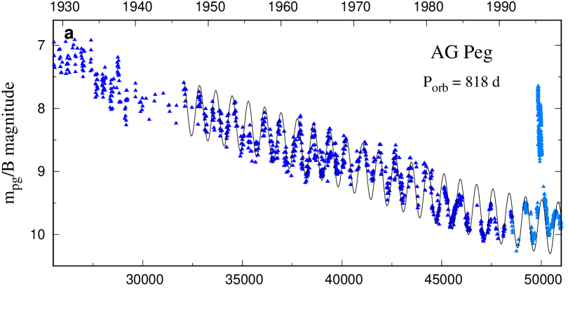
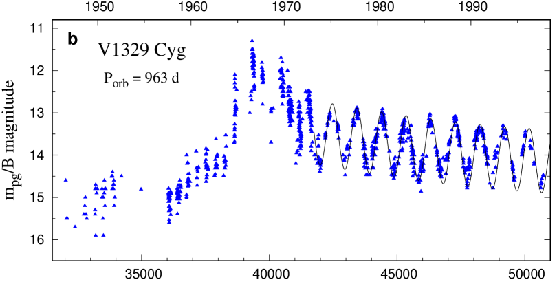
Figure 12: Transition from the symbiotic nova outburst to quiescent phase and eventually to Z And-type outburst for AG Peg, V1329 Cyg, and V426 Sge. The sine curve fits the wave-like orbitally related variation. a: Descending part of the historical LC of AG Peg from its 1850 symbiotic nova outburst. The 2015 Z And-type outburst is shifted by $-9\times P_{\rm orb}$ for a better comparison. Data are from Meinunger (1983) and Sekeráš et al. (2019). b: Historical LC of V1329 Cyg covering its symbiotic nova outburst around 1965. Data were summarised by Chochol et al. (1999). c: The 1968 symbiotic nova outburst ($m_{\rm pg}$ in blue) and the 2018 Z And-type outburst ($V$ in red) of V426 Sge. Data for the latter event are shifted by $-18\times P_{\rm orb}$ and +0.75 mag.

4.3.2 Accretion-powered symbiotics: Progenitors to symbiotic nova outbursts

The event of symbiotic nova outburst requires a long-lasting preceding accretion by the WD from the red giant wind to accumulate a sufficient amount of hydrogen-rich material to ignite a thermonuclear outburst on the surface of the WD (see Mürset & Nussbaumer (1994) and Bode & Evans (2008) for a review). Therefore, WDs in symbiotic binaries accreting in the nova regime (i.e. below the stable-burning limit; see e.g. Nomoto et al. 2007) are accretion-powered only, and thus represent progenitors to symbiotic nova outbursts; they are far less abundant among all the known symbiotics with only a few well-observed objects in the optical (e.g. EG And, 4 Dra, SU Lyn, see Skopal 2005b; Mukai et al. 2016). The accretion-powered symbiotics generate a low luminosity of $\sim 10^{1}-10^{2}$ $L_{\sun}$, and thus also a low flux of ionising photons. As a result, a faint nebular continuum with only a few emission lines (mostly H$\alpha$, H$\beta$ and some forbidden lines) are superposed on the red giant continuum in the optical. Examples for EG And were illustrated by Smith (1980), Munari (1993), and Kenyon & Garcia (2016), for CQ Dra by Wheatley et al. (2003) and Skopal (2005a) and for SU Lyn by Mukai et al. (2016) and Teyssier et al. (2019).

Their photometric variability in the optical is also low. Observed are 0.1–0.2 mag variations, which can be modulated with the orbit (EG And), and $\sim$0.1 mag oscillations probably caused by a variability of the giant (see the long-term photometry of EG And and CQ Dra by Sekeráš et al. 2019; Hric & Urban 1991; Hric et al. 1994). However, changes in the ultraviolet and X-rays can be significant, as recently reported for SU Lyn by Lopes de Oliveira et al. (2018), who measured a dramatic drop in the UV-to-X-ray luminosity ratio on a timescale of 9 months. The authors interpreted this event as being a consequence of the almost 90 % decrease in the accretion rate. This suggests that the activity of red giants in symbiotic stars is important for fueling their WDs, and can therefore be used to determine their evolutionary path.

4.3.3 Evolution from the symbiotic nova to the first Z And-type outburst

At a certain point during the decline from the symbiotic nova outburst, the sinusoidal variation develops along the orbit. This signals a gradual transition to quiescent phase, where a dense symbiotic nebula is represented by the ionised fraction of a slow massive wind from the cool giant (Sect. 1). The luminosity of the burning WD decreases to a few times $10^{3}$ $L_{\sun}$ at a high temperature of $1-2\times 10^{5}$ K (e.g. Mürset & Nussbaumer 1994), which generates a large flux of ionising photons ($\sim 10^{47}$ s^-1) giving rise to an extended nebula. The nebula occupies a significant part of the circumbinary environment, whose optically thick part is responsible for the pronounced sinusoidal variation along the orbit (Skopal 2001).

In the case of AG Peg, the nova outburst ceased around 1995, when the accretion process switched on and the decline in the brightness of the star levelled out showing the pronounced sinusoidal variation until the Z And-type outburst in June 2015 (see Skopal et al. 2017). During this $\sim$20 years of quiescence, the high $L_{\rm WD}$ of $2-3\times 10^{3}$ $L_{\sun}$ was sustained by the accretion in the stable-burning regime. Subsequently, an increase in the accretion rate above the upper limit of the stable-burning ignited the Z And-type outburst.

The same evolutionary path from symbiotic nova to Z And-type outburst is also indicated for V426 Sge by the same type of LC evolution (Fig. 12) and the parameters of the burning WD during its 2018 Z And-type outburst, which are similar to those determined for AG Peg (Sect. 4.1). Thus, V426 Sge also came to be a classical symbiotic star.

4.3.4 Connections between basic types of symbiotic stars

The above described evolution of V426 Sge and AG Peg from their symbiotic nova to Z And-type outbursts suggests that all classical symbiotic stars showing the well pronounced sinusoidal variation along the orbit have experienced a symbiotic nova outburst in the past. If we assume that the pronounced wave-like orbitally related variability, which develops after a symbiotic nova outburst, results from a high $L_{\rm WD}$ generated by the stable hydrogen burning on the WD surface, then the following connections between basic types of symbiotic stars can be considered.

1. If the giant is not capable of sustaining the stable burning, the shell burning from prior nova will gradually expire, resulting in a gradual fading of the symbiotic activity with significantly damped sinusoidal variation. EG And is an example here. The WD will accrete in the nova regime and the system will become accetion powered, giving rise to the next symbiotic nova outburst in future (Sect. 4.3.2). As this happens on very different timescales, from a few times $10^{5}$ years to that of human life (see, e.g. Yaron et al. 2005), only the recurrent symbiotic novae are regularly observed as a result of this path.

2. As long as the giant is capable of fueling the WD at the rate required by the stable burning, the pronounced wave-like variation will continue at a constant level. Here, all quiet symbiotic stars showing this type of variability (e.g. SY Mus, RW Hya, V443 Her, BD–21^∘3873) are found at this stage.

3. If the accretion rate temporarily exceeds the upper limit of the stable burning, the Z And-type outburst occurs (see Skopal et al. 2017, for details). Here, all the best-studied symbiotic stars whose LCs show the pronounced wave-like orbitally related variation during the quiescent phase and indicate at least one Z And-type outburst belong to this category. We call them classical symbiotic stars, and Z And is their prototype.

5 Summary

In this paper we primarily analyse the newly discovered 2018 outburst of V426 Sge using our high-cadence optical spectroscopy and multicolour photometry complemented with Swift-XRT and UVOT observations and NIR $JHKL$ photometry. Using the Moscow and Sonneberg photographic plate archives, we re-constructed the historical LC of V426 Sge from approximately the year 1900. The main results of our analysis can be summarised as follows.

1. From around 1900 to 1967, V426 Sge did not show any typical symbiotic-like activity. In 1968, V426 Sge experienced the symbiotic nova outburst that ceased around 1990. Similarly to other symbiotic novae (e.g. AG Peg and V1329 Cyg), a pronounced wave-like orbitally related variation developed in its LC, when returning from the nova outburst to quiescent phase (Figs. 1, 2 and 12). The corresponding period of $493.4\pm 0.7$ days is the orbital period of the binary (Eq. (1)).

2. After around 28 years of quiescence, at the beginning of August 2018, V426 Sge erupted again showing characteristics of a Z And-type outburst. Around maximum, the WD increased its temperature to $\ga 2\times 10^{5}$ K, generated luminosity of $(7\pm 1)\times 10^{37}\,(d/3.3\,{\rm kpc})^{2}$$\rm\,erg\,s^{-1}$ and blew a wind at the rate of $\sim 3\times 10^{-6}$ $M_{\sun}\,{\rm yr}^{-1}$, whose emission measure of $6-7\times 10^{60}\,(d/3.3\,{\rm kpc})^{2}$ cm^-3 was indicated by SED models (Figs. 4 and 5, Table 8). Quantities of these parameters are very close to those observed during the 2015 Z And-type outburst of the symbiotic nova AG Peg (see Sect. 4.1).

3. Around the middle of February 2019, V426 Sge came to quiescent phase, and began to develop wave-like variation along its orbit (Sect. 3.5, Figs. 9 and 1).

4. Our Swift-UVOT/optical SED model from the quiescent phase (on March 3, 2019) revealed a high $L_{\rm WD}$ of $\sim$2300 $L_{\sun}$ emitted at a high $T_{\rm WD}$ of $\approx$150 kK. This suggests that the accretor is a low-mass $\sim$0.5 $M_{\sun}$ WD burning hydrogen on its surface at steady state conditions (Table 9, Sect. 4.1).

5. Our optical/NIR SED models from the quiescent phase revealed that the donor is a normal (probably variable) M4.7($\pm$0.2) III red giant characterised with $T_{\rm eff}\sim 3\,400$ K, $R_{\rm G}\sim 106$ $R_{\sun}$  and $L_{\rm G}\sim 1350$ $L_{\sun}$ (Sect. 3.6, Fig. 10).

6. The cases of V426 Sge and AG Peg, where the symbiotic nova outburst was followed by the Z And-type outburst and similar evolution in their LCs, lead us to sketch out some possible connections between the basic types of symbiotic stars, as follows:

   Symbiotic nova outbursts result from prolonged accretion by the WD in an accretion-powered symbiotic star (Sect. 4.3.2). During the transition from the nova outburst to quiescent phase, a pronounced sinusoidal variation along the orbit develops in the LC (Sect. 4.3.1, Fig. 12). The following evolution depends on the accretion rate by the WD (Sect. 4.3.4).

   (i) If the giant is capable of sustaining stable hydrogen burning on the WD surface, the wave-like variability continues at a constant level: we observe quiet symbiotic stars.

   (ii) If the accretion exceeds the upper limit for the stable burning, a Z And-type outburst occurs and the system becomes a classical symbiotic star.

   (iii) If the giant is not capable of sustaining the stable burning, the system becomes accretion-powered, and the progenitor of a future symbiotic nova outburst.

Appendix A Tables with optical photometry of V426 Sge

Table 10: $UBVR_{\rm C}I_{\rm C}$ photometry of V426 Sge obtained at the Stará Lesná and Kolonica Saddle observatories. The full table is available at the CDS.

HJD	UT	$U$		$B$		$V$		$R_{\rm C}$		$I_{\rm C}$		Tel. ID
+2 458 000	yyyy mm dd.ddd	mag	error	mag	error	mag	error	mag	error	mag	error
343.357	2018 08 12.857	10.702	0.055	11.496	0.030	10.938	0.014	10.060	0.036	9.220	0.052	G2
344.342	2018 08 13.842	10.701	0.038	11.481	0.025	10.896	0.007	9.997	0.029	9.145	0.046	G2
344.348	2018 08 13.848			11.506	0.025	10.935	0.007	10.028	0.028	9.167	0.038	G1
347.337	2018 08 16.837	10.691	0.039	11.511	0.026	10.906	0.009	9.973	0.030	9.132	0.047	G2
348.396	2018 08 17.896			11.487	0.026	10.872	0.008	9.939	0.029			G1
348.406	2018 08 17.906	10.641	0.039	11.483	0.027	10.861	0.012	9.926	0.031	9.095	0.047	G2

Table 11: $BVR_{\rm C}I_{\rm C}$ photometry of V426 Sge obtained within the ANS collaboration. The full table is available at the CDS.

HJD	UT	$B$		$V$		$R_{\rm C}$		$I_{\rm C}$		Tel. ID
+2 458 000	yyyy mm dd.ddd	mag	error	mag	error	mag	error	mag	error
341.33743	2018 08 10.837	11.459	0.010	10.926	0.009	10.101	0.013	9.199	0.010	0310
342.46219	2018 08 11.962	11.414	0.010	10.872	0.010	10.042	0.009	9.153	0.011	0310
345.52123	2018 08 15.021	11.453	0.007	10.771	0.004			9.092	0.009	2100
345.55826	2018 08 15.058	11.444	0.008	10.843	0.007	10.007	0.009	9.124	0.011	0310
347.51701	2018 08 17.017	11.504	0.005	10.816	0.004			9.085	0.009	2100
348.40872	2018 08 17.909	11.476	0.011	10.873	0.010	9.985	0.013	9.112	0.012	0310

Table 12: Photographic magnitudes of V426 Sge obtained from archives. The full table is available at the CDS.

HJD	UT	$m_{\rm pg}$		Archive
+2 400 000	yyyy mm dd.ddd	mag	error
14578.264	1898 10 15.764	$>$13.8	not visible	M
14908.317	1899 09 10.817	$>$12.6	not visible	M
14909.375	1899 09 11.875	13.62	0.16	M
15614.344	1901 08 17.844	13.45	0.18	M
18950.246	1910 10 05.746	13.86	0.18	M
18973.220	1910 10 28.720	13.09	0.16	M
28751.397	1937 08 05.897	13.68	0.17	M

Appendix B Table of the used line fluxes

Table 13: Dereddened fluxes for the He ii 4686 Å, H$\beta$ and Raman scattered O vi 6825 Å lines in units of 10^-13$\rm\,erg\,s^{-1}\,cm^{-2}$.

UT	HJD	$F_{4686}$	error	$F_{{\rm H}\beta}$	error	$F_{\rm Raman}$	error
yyyy/mm/dd.ddd	+2 400 000
20180810.845	58341.345	162.5	12.2	125.4	9.4	0.00	–
20180811.826	58342.326	165.6	14.5	142.3	12.5	0.00	–
20180812.872	58343.372	–	–	–	–	0.00	–
20180813.814	58344.314	210.6	20.0	271.2	25.8	1.72	0.58
20180813.827	58344.327	239.4	22.0	245.8	22.5	1.72	0.58
20180815.853	58346.353	183.4	19.0	146.0	15.2	0.92	0.58
20180817.070	58347.570	144.2	18.0	128.2	16.0	1.25	0.77
20180817.896	58348.396	135.0	16.0	174.4	17.0	–	–
20180818.823	58349.323	212.2	20.0	237.4	22.4	0.95	0.67
20180819.842	58350.342	228.1	23.0	246.8	24.9	2.26	0.86
20180820.060	58350.560	192.6	20.2	–	–	2.23	0.67
20180820.868	58351.369	205.0	27.0	334.5	44.1	4.21	0.77
20180822.833	58353.333	–	–	–	–	6.42	1.54
20180822.840	58353.340	221.0	16.0	379.2	24.4	6.06	1.63
20180827.796	58358.296	206.0	22.5	369.5	40.3	6.99	0.77
20180907.867	58369.367	187.5	20.0	419.1	44.8	12.74	1.25
20180919.821	58381.321	238.6	17.5	511.6	37.6	16.00	1.63
20180920.837	58382.337	196.4	18.5	498.2	47.0	18.78	1.92
20180920.882	58382.382	–	–	–	–	13.60	1.44
20181004.840	58396.340	136.0	14.0	386.2	40.0	19.80	2.00
20181005.724	58397.224	166.1	18.0	346.8	37.5	21.75	2.20
20181010.788	58402.288	190.1	19.0	364.1	36.0	21.17	2.11
20181011.835	58403.335	108.2	22.0	261.5	50.0	16.50	1.70
20181016.713	58408.213	156.5	12.0	422.1	32.5	17.34	1.72
20181018.797	58410.297	122.8	13.0	200.3	21.0	15.52	1.53
20181020.757	58412.257	91.9	11.0	171.1	20.5	16.00	1.34
20181108.741	58431.241	124.6	19.0	–	–	16.19	1.63
20181110.773	58433.273	71.3	10.0	118.6	20.0	13.20	1.50
20181112.803	58435.303	58.2	4.8	132.5	11.0	14.85	1.53
20181123.729	58446.229	77.5	6.5	142.7	12.0	10.83	1.15
20181217.701	58470.201	46.9	5.0	78.4	8.3	8.54	0.86
Quiescent phase
20190623.872a	58658.372	29.2	3.5	24.7	3.0	3.6	0.7
20190625.931a	58660.431	28.8	3.5	23.3	3.0	3.8	0.7
20190819.832a	58715.332	32.2	4.0	25.2	3.0	3.2	0.6
20190907.191a	58733.691	35.8	4.0	29.6	3.0	3.6	0.4
20191005.112a	58761.612	36.5	4.0	38.1	4.0	3.7	0.5
20191113.760	58801.260	48.7	2.0	59.3	3.0	5.4	0.5

Notes. ^(a) low-resolution spectrum