Certified Global Minima for a Benchmark of Difficult Optimization Problems

Abstract

We provide the global optimization community with new optimality proofs for six deceptive benchmark functions (five bound-constrained functions and one nonlinearly constrained problem). These highly multimodal nonlinear test problems are among the most challenging benchmark functions for global optimization solvers; some have not been solved even with approximate methods.

The global optima that we report have been numerically certified using Charibde (Vanaret et al., 2013), a hybrid algorithm that combines an evolutionary algorithm and interval-based methods. While metaheuristics generally solve large problems and provide sufficiently good solutions with limited computation capacity, exact methods are deemed unsuitable for difficult multimodal optimization problems. The achievement of new optimality results by Charibde demonstrates that reconciling stochastic algorithms and numerical analysis methods is a step forward into handling problems that were up to now considered unsolvable.

We also provide a comparison with state-of-the-art solvers based on mathematical programming methods and population-based metaheuristics, and show that Charibde, in addition to being reliable, is highly competitive with the best solvers on the given test functions.

1 Introduction

Numerical solvers usually embed advanced methods to tackle nonlinear optimization problems. Stochastic methods, in particular evolutionary algorithms, handle large problems and provide sufficiently good solutions with limited computation capacity, but may easily get trapped in local minima. On the other hand, local and global (exhaustive) deterministic methods may guarantee local or global optimality, but are often limited by the size or the nonlinearity of the problems and may suffer from numerical approximations.

In [20], a new reliable hybrid solver named Charibde has been introduced to reconcile stochastic methods and numerical analysis methods. An evolutionary algorithm and an interval-based algorithm are combined in a cooperative framework: the two methods run in parallel and cooperate by exchanging the best known upper bound of the global minimum and the best current solution. The contribution of this paper is the achievement of new certified optimality results by Charibde for six highly multimodal nonlinear test functions, for which no or few results were available. We also compare Charibde with state-of-the art solvers including mathematical programming methods, population-based metaheuristics and spatial branch and bound. Charibde proves to be highly competitive with the best solvers on the given test functions, while being fully reliable.

Charibde is presented in Section 2. It is evaluated on a benchmark of difficult test functions given in Section 3. State-of-the-art solvers to which Charibde is compared are described in Section 4. Numerical results, including proofs of optimality, values of global minima and corresponding solutions, are provided and discussed in Section 5.

2 Charibde: a Rigorous Solver

The rigorous nonlinear solver Charibde was introduced by Vanaret et al. [20], building on an original idea by Alliot et al. [1]. It combines the efficiency of a Differential Evolution algorithm and the reliability of interval computations to discard more efficiently subspaces of the search-space that cannot contain a global minimizer. We introduce interval computations and interval-based methods in Sections 2.1 and 2.2. Details on the implementation of the Differential Evolution algorithm are given in Section 2.3. Finally, the cooperation scheme of Charibde is explained in Section 2.4.

2.1 Interval Analysis

Interval Analysis (IA) is a method of numerical analysis introduced by Moore [12] to bound rounding errors in floating-point computations. Real numbers that are not representable on a computer are enclosed within intervals with floating-point bounds. Each numerical computation is safely carried out by using outward rounding.

Definition 1.

An interval $X=[\underline{X},\overline{X}]$ is the set $\{x\in\mathbb{R}~{}|~{}\underline{X}\leq x\leq\overline{X}\}$. We denote by $m(X)=\frac{1}{2}(\underline{X}+\overline{X})$ its midpoint. $\mathbb{IR}$ is the set of all intervals. A box $\mathbf{X}=(X_{1},\ldots,X_{n})$ is an interval vector. We note $m(\mathbf{X})=(m(X_{1}),\ldots,m(X_{n}))$ its midpoint. In the following, capital letters represent interval quantities (interval $X$) and bold letters represent vectors (box $\mathbf{X}$, vector $\mathbf{x}$).

Interval arithmetic defines the interval counterparts of real-valued operators ($\{+,-,\times,/\}$) and elementary functions ($\exp$, $\cos$, $\ldots$). For example, $[a,b]+[c,d]=[a+_{\downarrow}c,b+_{\uparrow}d]$ and $\exp([a,b])=[\exp_{\downarrow}(a),\exp_{\uparrow}(b)]$, where $\cdot_{\downarrow}$ (resp. $\cdot_{\uparrow}$) denotes downward (resp. upward) rounding.

Definition 2.

Let $f:\mathbb{R}^{n}\rightarrow\mathbb{R}$ be a real-valued function. $F:\mathbb{IR}^{n}\rightarrow\mathbb{IR}$ is an interval extension of $f$ if

$$\forall\mathbf{X}\in\mathbb{IR}^{n},f(\mathbf{X})=\{f(\mathbf{x})~{}|~{}\mathbf{x}\in\mathbf{X}\}\subset F(\mathbf{X})$$

$$\forall(\mathbf{X},\mathbf{Y})\in\mathbb{IR}^{n},\mathbf{X}\subset\mathbf{Y}\Rightarrow F(\mathbf{X})\subset F(\mathbf{Y})$$

The natural interval extension $F_{N}$ is obtained by replacing elementary operations in $f$ with their interval extensions.

Dependency is the main source of overestimation when using interval computations: multiple occurrences of a same variable are considered as different variables. For example, the interval evaluation of $f(x)=x^{2}-2x$ over the interval $[1,4]$ yields $F_{N}([1,4])=[-7,14]$, which crudely overestimates the exact range $f([1,4])=[-1,8]$. However, an appropriate rewriting of the syntactic expression of $f$ may reduce or overcome dependency: if $f$ is continuous inside a box, $F_{N}$ yields the optimal range when each variable occurs only once in its expression. Completing the square in the expression of $f$ provides the optimal syntactic expression $g(x)=(x-1)^{2}-1$. Then $G_{N}([1,4])=[-1,8]=f([1,4])$.

2.2 Interval-based Techniques

2.2.1 Interval Branch and Bound Algorithms

Interval Branch and Bound algorithms (IB&B) exploit the conservative properties of interval extensions to rigorously bound global optima of numerical optimization problems [6]. The method consists in splitting the initial search-space into subspaces (branching) on which an interval extension is evaluated (bounding). By keeping track of the best upper bound $\tilde{f}$ of the global minimum $f^{*}$, boxes that certainly do not contain a global minimizer are discarded (example 1). Remaining boxes are stored to be processed at a later stage until the desired precision $\varepsilon$ is reached. The process is repeated until all boxes have been processed. Convergence certifies that $\tilde{f}-f^{*}<\varepsilon$, even in the presence of rounding errors. However, the exponential complexity of IB&B hinders the speed of convergence on large problems.

Example 1.

Consider the problem $\min\limits_{x\in X}f(x)=x^{4}-4x^{2}$ over $X=[-1,4]$. Then $F_{N}([-1,4])=[-64,256]\supset[-4,192]\\ =f([-1,4])$. The floating-point evaluation $f(1)=-3$ provides an upper bound $\tilde{f}$ of $f^{*}$. Evaluating $F_{N}$ on the subinterval $[3,4]$ reduces the overestimation induced by dependency: $F_{N}([3,4])=[17,220]\supset[45,192]=f([3,4])$. Because $\forall x\in[3,4],f(x)\geq 17>\tilde{f}=-3\geq f^{*}$, the interval $[3,4]$ cannot contain a global minimizer and can be safely discarded.

2.2.2 Interval Contraction

Propagating the (in)equality constraints of the problem, as well as the constraints $f\leq\tilde{f}$ and $\nabla f=0$, may narrow the domains of the variables or prove that a subdomain of the search-space cannot contain a global minimizer.

Stemming from the IA and Interval Constraint Programming communities, filtering/contraction algorithms [4] narrow the bounds of the variables without loss of solutions. Standard contraction algorithms generally integrate a filtering procedure into a fixed-point algorithm. HC4 [3] handles one constraint after the other and performs the optimal contraction w.r.t. to a constraint if variables occur only once in its expression. Box [19] narrows one variable after the other w.r.t. all constraints, using an interval version of Newton’s method. Mohc [2] exploits the monotonicity of the constraints to enhance contraction of HC4 and interval Newton.

The interval-based algorithm embedded in Charibde follows an Interval Branch and Contract (IB&C) scheme (algorithm 1) that interleaves steps of bisection and filtering. We note $\mathcal{L}$ the priority queue in which the remaining boxes are stored, $\varepsilon$ the desired precision and $\tilde{x}$ the best known solution, such that $\overline{F(\tilde{x})}=\tilde{f}$.

Algorithm 1 Interval Branch and Contract framework

$\tilde{f}\leftarrow+\infty$ $\triangleright$ best found upper bound

$\mathcal{L}\leftarrow\{\mathbf{X}_{0}\}$ $\triangleright$ priority queue of boxes to process

repeat

     Extract a box $\mathbf{X}$ from $\mathcal{L}$ $\triangleright$ selection rule

     Compute $F(\mathbf{X})$ $\triangleright$ bounding rule

     if $\mathbf{X}$ cannot be eliminated then $\triangleright$ cut-off test

         Contract$(\mathbf{X},\tilde{f})$ $\triangleright$ filtering algorithms

         Compute $F(m(\mathbf{X}))$ to update $\tilde{f}$ $\triangleright$ midpoint test

         Bisect $\mathbf{X}$ into $\mathbf{X}_{1}$ and $\mathbf{X}_{2}$ $\triangleright$ branching rule

         Store $\mathbf{X}_{1}$ and $\mathbf{X}_{2}$ in $\mathcal{L}$

     end if

until $\mathcal{L}=\varnothing$

return $(\tilde{f},\tilde{x})$

2.3 Differential Evolution

Differential Evolution (DE) is an Evolutionary Algorithm that combines the coordinates of existing individuals with a particular probability to generate new potential solutions [17]. It was embedded within Charibde for its ability to solve extremely difficult optimization problems, while having few control parameters.

We denote by $NP$ the population size, $W>0$ the weighting factor and $CR\in[0,1]$ the crossover rate. For each individual $\mathbf{x}$ of the population, three other individuals $\mathbf{u}$, $\mathbf{v}$ and $\mathbf{w}$, all different and different from $\mathbf{x}$, are randomly picked in the population. The newly generated individual $\mathbf{y}=(y_{1},\ldots,y_{j},\ldots,y_{n})$ is computed as follows:

$$y_{j}=\begin{cases}u_{j}+W\times(v_{j}-w_{j})&\text{ if }j=R\text{ or }r_{j}<CR\\ x_{j}&\text{ otherwise}\end{cases}$$ (1)

where $R$ is a random index in $\{1,\ldots,n\}$ ensuring that at least one component of $\mathbf{y}$ differs from that of $\mathbf{x}$, and $r_{j}$ is a random number uniformly distributed in $[0,1]$, picked for each $y_{j}$. $\mathbf{y}$ replaces $\mathbf{x}$ in the population if $f(\mathbf{y})<f(\mathbf{x})$.

The following advanced rules have been implemented in Charibde:

Boundary constraints:

When a component $y_{j}$ lies outside the bounds $[\underline{X_{j}},\overline{X_{j}}]$ of the search-space, the bounce-back method [16] replaces $y_{j}$ with a component that lies between $u_{j}$ and the admissible bound:

$$\small y_{j}=\begin{cases}u_{j}+rand(0,1)(\overline{X_{j}}-u_{j}),&\text{if }y_{j}>\overline{X_{j}}\\ u_{j}+rand(0,1)(\underline{X_{j}}-u_{j}),&\text{if }y_{j}<\underline{X_{j}}\end{cases}$$ (2)

Evaluation:

Given inequality constraints $\{g_{i}~{}|~{}i=1,\ldots,m\}$, the evaluation of an individual $\mathbf{x}$ is computed as a triplet ($f_{\mathbf{x}}$, $n_{\mathbf{x}}$, $s_{\mathbf{x}}$), where $f_{\mathbf{x}}$ is the objective value of $\mathbf{x}$, $n_{\mathbf{x}}$ the number of violated constraints and $s_{\mathbf{x}}=\sum_{i=1}^{m}\max(g_{i}(\mathbf{x}),0)$. If at least one of the constraints is violated, the objective value is not computed

Selection:

Given the evaluation triplets ($f_{\mathbf{x}},n_{\mathbf{x}},s_{\mathbf{x}}$) and ($f_{\mathbf{y}},n_{\mathbf{y}},s_{\mathbf{y}}$) of two candidate solutions $\mathbf{x}$ and $\mathbf{y}$, the best individual to be kept for the next generation is computed as follows:

• if $n_{\mathbf{x}}<n_{\mathbf{y}}$ or ($n_{\mathbf{x}}=n_{\mathbf{y}}>0$ and $s_{\mathbf{x}}<s_{\mathbf{y}}$) or ($n_{\mathbf{x}}=n_{\mathbf{y}}=0$ and $f_{\mathbf{x}}<f_{\mathbf{y}}$) then $\mathbf{x}$ is kept

• otherwise, $\mathbf{y}$ replaces $\mathbf{x}$

2.4 Charibde: a Cooperative Algorithm

Charibde combines an Interval Branch and Contract algorithm and a Differential Evolution algorithm in a cooperative way: neither of the algorithms is embedded within the other, but they run in parallel and exchange bounds and solutions using an MPI implementation (Figure 1).

Figure 1: Basic scheme of cooperation

The cooperation scheme boils down to 3 main steps:

• Whenever the best known DE evaluation is improved, the best individual $\mathbf{x}_{b}$ is evaluated using IA. The upper bound of the image $\overline{F(\mathbf{x}_{b})}$ – an upper bound of the global minimum – is sent to the IB&C thread

• In the IB&C algorithm, $\overline{F(\mathbf{x}_{b})}$ is compared to the current best upper bound $\tilde{f}$. An improvement of the latter leads to a more efficiently pruning of the subspaces that cannot contain a (feasible) global minimizer

• Whenever the evaluation of the center $m(\mathbf{X})$ of a box improves $\tilde{f}$, the individual $m(\mathbf{X})$ replaces the worst individual of DE, thus preventing premature convergence

3 Benchmark of Test Functions

The highly multimodal nonlinear test functions considered in this study can be found in Table 1. Contrary to standard test functions that have a global minimum 0 at $(0,\ldots,0)$ (Griewank function) or have a global minimizer with $n$ identical components (Schwefel function), we have selected six functions with nontrivial global minima: Michalewicz function, Sine Envelope Sine Wave function (shortened to Sine Envelope), Shekel’s Foxholes function [16], Egg Holder function [21], Rana’s function [21] and Keane’s function [8]. Except for the Michalewicz function, all are nonseparable. Their surfaces and contour lines can be observed on Figure 2 for $n=2$. It illustrates the numerous local minima and the ruggedness of the functions.

The first inequality constraint of Keane’s function describes a hyperbola in two dimensions and is active at the global minimizer, which hinders the efficiency of solvers. The second inequality constraint is linear and is not active at the global minimizer. The Egg Holder (resp. Rana) function is strongly subject to dependency: $x_{1}$ and $x_{n}$ occur three (resp. five) times in its expression, and $(x_{2},\ldots,x_{n-1})$ occur six (resp. ten) times. Its natural interval extension therefore produces a large overestimation of the actual range.

The last three functions (Egg Holder, Rana and Keane) contain absolute values. $|\cdot|$ is differentiable everywhere except for $x=0$, however its subderivative – generalizing the derivative to non-differentiable functions – at $x=0$ can be computed. Charibde handles an interval extension proposed by Kearfott [9], based on the values of its subderivative:

$$|\cdot|^{\prime}(X)=\begin{cases}[-1,-1]&\text{ if }\overline{X}<0\\ [1,1]&\text{ if }\underline{X}>0\\ [-1,1]&\text{otherwise}\end{cases}$$ (3)

This expression is used to compute an enclosure of the partial derivatives of $f$ through automatic differentiation.

Table 1: Test functions

Function	Expression	Domain
Michalewicz	$-\sum_{i=1}^{n}\sin(x_{i})\left[\sin(\frac{ix_{i}^{2}}{\pi})\right]^{20}$	$[0,\pi]^{n}$
Sine Envelope	$-\sum_{i=1}^{n-1}\left(0.5+\frac{\sin^{2}(\sqrt{x_{i+1}^{2}+x_{i}^{2}}-0.5)}{(0.001(x_{i+1}^{2}+x_{i}^{2})+1)^{2}}\right)$	$[-100,100]^{n}$
Shekel	$-\sum_{i=1}^{30}\frac{1}{c_{i}+\sum_{j=1}^{n}(x_{j}-a_{ij})^{2}}$	$[0,10]^{n}$
Egg Holder	$-\sum_{i=1}^{n-1}\left[(x_{i+1}+47)\sin\left(\sqrt{|x_{i+1}+47+\frac{x_{i}}{2}|}\right)+x_{i}\sin\left(\sqrt{|x_{i}-(x_{i+1}+47)|}\right)\right]$	$[-512,512]^{n}$
Rana	$\sum_{i=1}^{n-1}(x_{i}\cos\sqrt{|x_{i+1}+x_{i}+1|}\sin\sqrt{|x_{i+1}-x_{i}+1|}+(1+x_{i+1})\sin\sqrt{|x_{i+1}+x_{i}+1|}\cos\sqrt{|x_{i+1}-x_{i}+1|})$	$[-512,512]^{n}$
Keane	$-\frac{|\sum_{i=1}^{n}\cos^{4}x_{i}-2\prod_{i=1}^{n}\cos^{2}x_{i}|}{\sqrt{\sum_{i=1}^{n}ix_{i}^{2}}}$ s.t. $0.75\leq\prod_{i=1}^{n}x_{i}$ and $\sum_{i=1}^{n}x_{i}\leq 7.5n$	$[0,10]^{n}$

(a) Michalewicz function

(b) Sine Envelope function

(c) Shekel’s Foxholes function

(d) Egg Holder function

(e) Rana’s function

(f) Keane’s function

Figure 2: Test functions ($n=2$)

4 State-of-the-art Solvers

The certified global minima obtained by Charibde are compared with state-of-the-art optimization softwares available on the NEOS (Network-Enabled Optimization System) server, a free web service for solving optimization problems in AMPL/GAMS formats. These solvers include local methods, population-based metaheuristics and spatial branch and bound: Ipopt implements a primal-dual interior point algorithm, which uses a filter line search method. LOQO is based on an infeasible primal-dual interior-point method. MINOS employs a reduced-gradient method. PGAPack is a Parallel Genetic Algorithm library. PSwarm combines pattern search and particle swarm. Couenne uses a reformulation-based branch-and-bound algorithm for a globally optimum solution. It is a complete solver, i.e. it performs an exhaustive exploration of the search-space.

Note: the solver BARON (Branch and Reduce Optimization Navigator), combining constraint propagation, interval analysis and duality, is known as one of the most efficient, although unreliable (see Section 5.3), solvers for solving nonconvex optimization problems to global optimality. However, it is not designed to handle trigonometric functions, and therefore will not be considered in this paper.

5 Numerical Experiments

5.1 Global Minima Certified by Charibde

The global minima to the six test functions are given in Table 6. All solutions are given with a precision $\varepsilon=10^{-6}$. Should the functions have several global minima, only one is provided. A reference given next to a global minimum indicates that a result is available in the literature.

Analyzing the results has brought out identities for finding putative minima for four of the six test functions. They can be found in Table 2.

Table 2: Putative minima

Function	Putative minimum	$R^{2}$
Michalewicz	$-0.99864n+0.30271$	0.9999981
Sine Envelope	$-1.49150n+1.49150$	1
Egg Holder	$-915.61991n+862.10466$	0.9999950
Rana’s	$-511.70430n+511.68714$	1

The global minima of the Michalewicz function for up to 75 variables can be found in Table 3. For the sake of conciseness, the corresponding solutions for up to only 10 variables are given in Table 6.

Table 3: Certified global minima of Michalewicz function

$n$	Global minimum	$n$	Global minimum
10	-9.6601517 [11]	45	-44.6256251
15	-14.6464002	50	-49.6248323 [11]
20	-19.6370136 [11]	55	-54.6240533
25	-24.6331947	60	-59.6231462
30	-29.6308839 [11]	65	-64.6226167
35	-34.6288550	70	-69.6222202
40	-39.6267489	75	-74.6218112

To illustrate the key role played by the syntactic expression of the function when computing with intervals, we have tested two different – but equivalent – syntaxes of Rana’s function in Charibde. The first syntax is given in Table 1. The second syntax is obtained using the trigonometric identity: $\cos x\sin y=\frac{1}{2}(\sin(x+y)-\sin(x-y))$. Their impact on the sharpness of the inclusions, therefore on the convergence of Charibde, can be observed in Table 4. The hyphen indicates a computing time greater than one hour.

Table 4: Rana’s function: CPU times (s) of convergence in Charibde ($NP=70$, $W=0.7$, $CR=0.5$)

$n$	CPU time (s)
	First syntax	Second syntax
2	0.25	0.009
3	6.5	0.12
4	254	1.45
5	-	18.5
6	-	244
7	-	3300

5.2 Comparison of Solvers

The comparison of the seven solvers on a particular instance of each test function can be found in Table 5. When available, the number of evaluations of the objective function is given under the found minimum, otherwise we have mentioned the computing time. The hyphens in the last column indicate that PGAPack and PSwarm cannot handle inequality constraints.

Local methods based on mathematical programming (Ipopt, LOQO, MINOS) usually require few iterations to reach a local minimum from a starting point. The quality of the minimum generally depends on both the starting point and the size of the basins of attraction of the function. These solvers turn out to perform poorly on the considered multimodal problems.

Among the population-based metaheuristics, PGAPack performs consistently better than PSwarm, yet at a higher cost. We have kept the best result ouf of five runs, since it is tedious to run an online solver several times. The default NEOS control parameters have been used; both algorithms would certainly perform better with suitable control parameters. The results of Couenne are discussed in Section 5.3.

Charibde achieves convergence in finite time on the six problems, with a numerical certification of optimality. It benefits from the start of convergence of the DE algorithm that computes a good initial value for $\tilde{f}$. This allows the IB&C algorithm to prune more efficiently subspaces of the search-space. The number of evaluations of the natural interval extension $F$ has the form $NE_{DE}+NE_{IB\&C}$, where $NE_{DE}$ is the number of evaluations in the DE algorithm (whenever the best known solution is improved) and $NE_{IB\&C}$ is the number of evaluations in the IB&C algorithm. Note that after converging toward the global minimizer, the DE thread keeps running as long as the certification of optimality has not been obtained.

Table 5: State-of-the-art solvers against Charibde on test functions

	Michalewicz	Sine Envelope	Shekel	Egg Holder	Rana	Keane
	($n=50$)	($n=5$)	($n=5$)	($n=5$)	($n=5$)	($n=4$)
Ipopt	-19.773742	-5.8351843	-1.8296708	-3586.3131827	-75.512076	-0.2010427
	(167 eval)	(24 eval)	(15 eval)	(8 eval)	(16 eval)	(8 eval)
LOQO	-0.0048572	-5.8351843	-1.9421143	25.5609238	-69.5206	-0.0983083
	(88 eval)	(17 eval)	(19 eval)	(5924 eval)	(138 eval)	(50 eval)
MINOS	0	-5.87878	-2.5589419	-3586.313183	-233.592	-0.2347459
	(3 eval)	(38 eval)	(3 eval)	(3 eval)	(1 eval)	(3 eval)
PGAPack	-37.60465	-5.569544	-1.829452	-3010.073	-2091.068	-
	(9582 eval)	(9615 eval)	(9602 eval)	(9626 eval)	(9622 eval)	-
PSwarm	-24.38158	-5.835182	-1.610072	-2840.799	-1595.056	-
	(2035 eval)	(2049 eval)	(2008 eval)	(2040 eval)	(2046 eval)	-
Couenne	-49.619042	-5.9660007	-10.4039521	-3719.7287498	-2046.8320657	-0.6222999
	(265s)	(0.4s)	(8s)	(20.6s)	(20.3s)	(2s)
Charibde	-49.6248323	-5.9659811	-10.4039521	-3719.7248363	-2046.8320657	-0.6222810
CPU time	8.4s	219s	0.04s	0.8s	17.8s	14860s
$f$ evaluations	717100	227911400	8150	742600	19186150	6351693297
$F$ evaluations	763 + 409769	93 + 21744667	28 + 561	106 + 82751	53 + 1383960	74 + 2036988566
($NP,W,CR$)	(50, 0.7, 0)	(50, 0.7, 0.9)	(50, 0.7, 0.9)	(50, 0.7, 0.4)	(50, 0.7, 0.5)	(70, 0.7, 0.9)

5.3 Reliability vs Efficiency

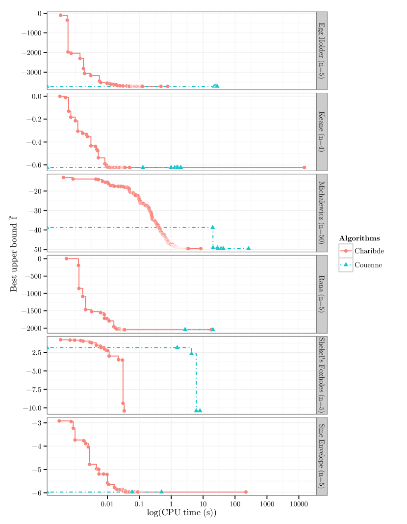
On Figure 3, the evolution of the best known solution in Charibde is compared with that of Couenne for a particular instance of each test function. Intermediate times for other solvers were not available. Note that the scale on the x-axis is logarithmic. These diagrams show that Charibde is highly competitive against Couenne: Charibde achieves convergence faster than Couenne on Michalewicz (ratio 31), Shekel (ratio 200), Egg Holder (ratio 25) and Rana’s function (ratio 1.1). Couenne is faster than Charibde on Sine Envelope (ratio 547) and Keane’s function (ratio 7430).

Is is however crucial to note that Couenne, while being a complete solver (the whole search-space is exhaustively processed), is not reliable. This stems from the fact that the under- and overestimators obtained by linearizing the function may suffer from numerical approximations. Contrary to interval arithmetic that bounds rounding errors, mere real-valued linearizations are not conservative and cannot guarantee the correctness of the result. This problem can easily be observed in Table 5: the global minima obtained by Couenne on Michalewicz, Sine Envelope, Egg Holder and Keane’s function are not correct compared to the certified minima provided by Charibde. The wrong decimal places are underlined.

6 Conclusion

We provided a comparison between Charibde, a cooperative solver that combines an EA and interval-based methods, and state-of-the-art solvers (stemming from mathematical programming and population-based metaheuristics). They were evaluated on a benchmark of nonlinear multimodal optimization problems among the most challenging: Michalewicz, Sine Envelope, Shekel’s Foxholes, Egg Holder, Rana and Keane. Charibde proved to be highly competitive with the best solvers, including Couenne, a complete but unreliable solver based on spatial branch and bound and linearizations. We provided new certified global minima for the considered test functions, as well as the corresponding solutions. They may be used from now on as references to test stochastic or deterministic optimization methods.

Table 6: Certified global minima

Function	$n$	Global minimum	Corresponding solution
Michalewicz	2	-1.8013034	(2.202906, 1.570796)
	3	-2.7603947	(2.202906, 1.570796, 1.284992)
	4	-3.6988571	(2.202906, 1.570796, 1.284992, 1.923058)
	5	-4.6876582	(2.202906, 1.570796, 1.284992, 1.923058, 1.720470)
	6	-5.6876582	(2.202906, 1.570796, 1.284992, 1.923058, 1.720470, 1.570796)
	7	-6.6808853	(2.202906, 1.570796, 1.284992, 1.923058, 1.720470, 1.570796, 1.454414)
	8	-7.6637574	(2.202906, 1.570796, 1.284992, 1.923058, 1.720470, 1.570796, 1.454414, 1.756087)
	9	-8.6601517	(2.202906, 1.570796, 1.284992, 1.923058, 1.720470, 1.570796, 1.454414, 1.756087, 1.655717)
	10	-9.6601517	(2.202906, 1.570796, 1.284992, 1.923058, 1.720470, 1.570796, 1.454414, 1.756087, 1.655717, 1.570796)
Sine Envelope	2	-1.4914953 [15]	(-0.086537, 2.064868)
	3	-2.9829906	(1.845281, -0.930648, 1.845281)
	4	-4.4744859	(2.066680, 0.001365, 2.066680, 0.001422)
	5	-5.9659811	(-1.906893, -0.796823, 1.906893, 0.796823, -1.906893)
	6	-7.4574764	(-1.517016, -1.403507, 1.517016, -1.403507, -1.517015, 1.403507)
Shekel	2	-12.1190084 [10]	(8.024065, 9.146534)
	3	-11.0307623	(8.024161, 9.150962, 5.113211)
	4	-10.4649942	(8.024876, 9.151655, 5.113888, 7.620843)
	5	-10.4039521 [5]	(8.024917, 9.151728, 5.113927, 7.620861, 4.564085)
	6	-10.3621514	(8.024916, 9.151795, 5.113951, 7.620875, 4.564063, 4.710999)
	7	-10.3131505	(8.024945, 9.151838, 5.113968, 7.620912, 4.564052, 4.711004, 2.996069)
	8	-10.2793068	(8.024947, 9.151874, 5.113979, 7.620933, 4.564043, 4.711003, 2.996055, 6.125980)
	9	-10.2288309	(8.024961, 9.151914, 5.113990, 7.620956, 4.564025, 4.710999, 2.996038, 6.125996, 0.734065)
	10	-10.2078768 [14]	(8.024968, 9.151929, 5.113991, 7.620959, 4.564020, 4.711005, 2.996030, 6.125993, 0.734057, 4.981999)
Egg Holder	2	-959.6406627 [13]	(512, 404.231805)
	3	-1888.3213909	(481.462894, 436.929541, 451.769713)
	4	-2808.1847922	(482.427433, 432.953312, 446.959624, 460.488762)
	5	-3719.7248363	(485.589834, 436.123707, 451.083199, 466.431218, 421.958519)
	6	-4625.1447737	(480.343729, 430.864212, 444.246857, 456.599885, 470.538525, 426.043891)
	7	-5548.9775483	(483.116792, 438.587598, 453.927920, 470.278609, 425.874994, 441.797326, 455.987180)
	8	-6467.0193267	(481.138627, 431.661180, 445.281208, 458.080834, 472.765498, 428.316909, 443.566304, 457.526007)
	9	-7376.2797668	(482.785353, 438.255330, 453.495379, 469.651208, 425.235102, 440.658933, 454.142063, 468.699867, 424.215061)
	10	-8291.2400675	(480.852413, 431.374221, 444.908694, 457.547223, 471.962527, 427.497291, 442.091345, 455.119420, 469.429312, 424.940608)
Rana	2	-511.7328819 [18]	(-488.632577, 512)
	3	-1023.4166105	(-512, -512, -511.995602)
	4	-1535.1243381	(-512, -512, -512, -511.995602)
	5	-2046.8320657	(-512, -512, -512, -512, -511.995602)
	6	-2558.5397934	(-512, -512, -512, -512, -512, -511.995602)
	7	-3070.2475210	(-512, -512, -512, -512, -512, -512, -511.995602)
Keane	2	-0.3649797 [7]	(1.600860, 0.468498)
	3	-0.5157855 [7]	(3.042963, 1.482875, 0.166211)
	4	-0.6222810 [7]	(3.065318, 1.531047, 0.405617, 0.393987)

Figure 3: Comparison of Couenne and Charibde (logarithmic x scale)

References

- [1] J.-M. Alliot, N. Durand, D. Gianazza, and J.-B. Gotteland. Finding and proving the optimum: Cooperative stochastic and deterministic search. 20th European Conference on Artificial Intelligence, 2012.
- [2] I. Araya, G. Trombettoni, and B. Neveu. Exploiting monotonicity in interval constraint propagation. In Proc. AAAI, pages 9–14, 2010.
- [3] F. Benhamou, F. Goualard, L. Granvilliers, and J.-F. Puget. Revising hull and box consistency. In International Conference on Logic Programming, pages 230–244. MIT press, 1999.
- [4] G. Chabert and L. Jaulin. Contractor programming. Artificial Intelligence, 173:1079–1100, 2009.
- [5] Q. Feng, S. Liu, G. Tang, L. Yong, and J. Zhang. Biogeography-based optimization with orthogonal crossover. Mathematical Problems in Engineering, 2013, 2013.
- [6] E. Hansen. Global optimization using interval analysis. Dekker, 1992.
- [7] L. Kang, Z. Kang, Y. Li, and H. de Garis. A two level evolutionary modeling system for financial data. In GECCO, pages 1113–1118, 2002.
- [8] A. Keane. Bump, a hard(?) problem. http://www.southampton.ac.uk/~ajk/bump.html, 1994.
- [9] R. B. Kearfott. Interval extensions of non-smooth functions for global optimization and nonlinear systems solvers. Computing, 57:57–149, 1996.
- [10] S. Koullias. Methodology for global optimization of computationally expensive design problems, 2013.
- [11] S. K. Mishra. Some new test functions for global optimization and performance of repulsive particle swarm method. Technical report, University Library of Munich, Germany, 2006.
- [12] R. E. Moore. Interval Analysis. Prentice-Hall, 1966.
- [13] Z. Oplatková. Metaevolution - Synthesis of Evolutionary Algorithms by Means of Symbolic Regression. PhD thesis, Tomas Bata University in Zlín, 2008.
- [14] J. P. Pedroso. Simple metaheuristics using the simplex algorithm for non-linear programming. In Engineering Stochastic Local Search Algorithms. Designing, Implementing and Analyzing Effective Heuristics, pages 217–221. Springer, 2007.
- [15] J. Pohl, V. Jirsík, and P. Honzík. Stochastic optimization algorithm with probability vector in mathematical function minimization and travelling salesman problem. WSEAS Trans. Info. Sci. and App., 7:975–984, 2010.
- [16] K. Price, R. Storn, and J. Lampinen. Differential Evolution - A Practical Approach to Global Optimization. Natural Computing. Springer-Verlag, 2006.
- [17] R. Storn and K. Price. Differential evolution - a simple and efficient heuristic for global optimization over continuous spaces. Journal of Global Optimization, pages 341–359, 1997.
- [18] J. Tao and N. Wang. DNA computing based RNA genetic algorithm with applications in parameter estimation of chemical engineering processes. Computers & Chemical Engineering, 31(12):1602 – 1618, 2007.
- [19] P. Van Hentenryck. Numerica: a modeling language for global optimization. In Proceedings of the Fifteenth international joint conference on Artifical intelligence - Volume 2, IJCAI’97, pages 1642–1647, 1997.
- [20] C. Vanaret, J.-B. Gotteland, N. Durand, and J.-M. Alliot. Preventing premature convergence and proving the optimality in evolutionary algorithms. In Proceedings of the Biennial International Conference on Artificial Evolution (EA-2013), 2013.
- [21] D. Whitley, K. Mathias, S. Rana, and J. Dzubera. Evaluating evolutionary algorithms. Artificial Intelligence, 85:245–276, 1996.