Jaynes-Cummings model under monochromatic driving

Abstract

We study analytically and numerically the properties of Jaynes-Cummings model under monochromatic driving. The analytical results allow to understand the regime of two branches of multi-photon excitation in the case of close resonance between resonator and driven frequencies. The rotating wave approximation allows to reduce the description of original driven model to an effective Jaynes-Cummings model with strong coupling between photons and qubit. The analytical results are in a good agreement with the numerical ones even if there are certain deviations between the theory and numerics in the close vicinity of the resonance. We argue that the rich properties of driven Jaynes-Cummings model represent a new area for experimental investigations with superconducting qubits and other systems.

I Introduction

The Jaynes-Cummings model (JCM) jc is the cornerstone system of quantum optics describing interactions of resonator photons with an atom, considered in a two-level approximation. The usual experimental conditions correspond to a weak coupling constant between photons and atom. In this regime the quantum evolution of the system is integrable demonstrating revival energy exchange between photons and atom jc ; eberly ; eberlybook ; scully . Such revival behavior had been first observed in experiments with Rydberg atoms inside a superconducting cavity walther . The overview of applications of JCM for various physical systems is given in jkono ; noriphysrep .

With the appearance of long living superconducting qubits esteve the coupling of such a qubit (or an artificial two-level atom) to microwave photons of cavity quantum electrodynamics (QED resonator or oscillator) became an active field of experimental research wendin . Thus single artificial-atom lasing astafiev and a nonlinearity of QED system fink have been realized and tested experimentally. In the frame of QED coupling between qubit and resonator it is very natural to consider the case of resonator pumping by a monochromatic microwave field (see e.g. astafiev ; ilichev ; buisson ). Thus the problem of monochromatically driven resonator with photons coupled to a qubit represents an interesting fundamental extension of JCM. This system can be viewed as a quantum monochromatically driven oscillator coupled to a qubit (or two-level atom or spin-1/2).

The first studies of JCM under monochromatic driving had been performed for the case of a dissipative quantum oscillator studied numerically in the frame of quantum trajectories zsprl . It was shown that under certain conditions the qubit is synchronized with the phase of monochromatic driving providing an example of quantum synchronization in this, on a first glance, rather simple system. The unusual regime of bistability induced by quantum tunneling has been reported which still requires a better understanding zsprl ; mavrogordatos . It was shown that many photons can be excited even at a relatively weak driving amplitude. It was also shown that two different qubits can be synchronized and entangled by the driving under certain conditions zsprb . Thus the driven JCM represents a very interesting example of a fundamental problem of quantum synchronization zssync . From the discovery of synchronization by Christian Huygens in 1665 huygens this fundamental nonlinear phenomenon has been observed and studied in a variety of real systems described by the classical dynamics pikovsky . At present the development of quantum technologies and especially superconducting qubits led to a significant growth of interest to the phenomenon of quantum synchronization (see e.g. bruder1 ; bruder2 ; bruder3 and Refs. there in). Thus the interest to the JCM under driving is growing with appearance of new experiments (see e.g. devoret ; paraoanu ; eschner ). The theoretical investigations by different groups are also in progress zsprl ; mavrogordatos ; fischer ; nori .

We note that the unitary evolution of driven JCM has been considered in refereeref1 in the rotating wave approximation (RWA) for the specific resonance case showing that above a certain driving border the Floquet eigenstates are not normalizable. In refereeref2 the comparison was done between the RWA and non-RWA evolution has been considered showing the existence of certain difference between these two cases.

With the aim of deeper understanding of the properties of driven JCM we study here the nondissipative case when the system evolution is described by the quantum time-dependent Hamiltonian and the related Schrodinger equation. We present here the comparative analysis of analytical and numerical treatment of this system. We develop the semiclassical description of quantum evolution considering mainly the case of close (but not exact) resonance driving with high excitation of oscillator states.

The paper is organized as follows: in Section II, we give the system description, the analytical analysis is described in Section III, the numerical results are presented in Section IV, the time evolution of coherent states is described in Section V, discussion of results and conclusion are given in Section VI. Appendix provides additional complementary material.

II System description

The monochromatically driven JCM is described by the Hamiltonian already considered in zsprl :

$$\hat{H}=\omega_{0}\hat{n}+\frac{\Omega}{2}\hat{\sigma}_{z}+g\omega_{0}(\hat{a}+\hat{a}^{\dagger})\hat{\sigma}_{x}+f\cos{(\omega t)}(\hat{a}+\hat{a}^{\dagger})$$ (1)

where $\hat{\sigma}_{i}$ are the usual Pauli operators describing a qubit, $g$ is a dimensionless coupling constant, the driving force amplitude and frequency are $f$ and $\omega$, the oscillator frequency is $\omega_{0}$ and $\Omega$ is the qubit energy spacing. The operators $\hat{a},\hat{a}^{\dagger}$ describe the quantum oscillator with number of photons being $\hat{n}=\hat{a}^{\dagger}\hat{a}$ ($\hat{n}|n\rangle=n|n\rangle$). Here and in the following we take $\hbar=1$.

In the RWA the Hamiltonian (1) takes the form:

$$\hat{H}=\omega_{0}\hat{n}+\frac{\Omega}{2}\hat{\sigma}_{z}+g\omega_{0}(\hat{a}\hat{\sigma}_{+}+\hat{a}^{\dagger}\hat{\sigma}_{-})+\frac{f}{2}(\hat{a}e^{i\omega t}+\hat{a}^{\dagger}e^{-i\omega t})\;.$$ (2)

The Floquet theory can be applied to the time periodic Hamiltonians (1) and (2) that gives the Floquet eigenstates ($|\Psi_{j}(t)\rangle$) and Floquet modes ($|\Phi_{j}(t)\rangle$)

$$|\Psi_{j}(t)\rangle=\exp{(-i\varepsilon_{j}t/\hbar)}|\Phi_{j}(t)\rangle$$ (3)

where $\varepsilon_{j}$ are quasienergy levels defined in the interval $[0,2\pi/T]$ and $|\Phi_{j}(t)\rangle=|\Phi_{j}(t+T)\rangle$ are periodic in time.

In the rotating frame the time dependence can be eliminated. Thus a state $|\Psi\rangle$, evolving via the Schrodinger equation $i\hbar\partial_{t}\Psi=H\Psi$, can be transformed to $|\tilde{\Psi}\rangle=\hat{U}^{\dagger}|\Psi\rangle=\exp\left(i\hat{A}t/\hbar\right)|\Psi\rangle$ where $\hat{U}^{\dagger}$ is a unitary operator generated by a Hermitian operator $\hat{A}=\omega(\hat{a}^{\dagger}\hat{a}+\hat{\sigma}_{+}\hat{\sigma}_{-})$. Then the system in the rotating frame of RWA is described by the transformed stationary Hamiltonian

$$\hat{H}_{r}=\Delta_{0}\hat{n}+\frac{\Delta_{\Omega}}{2}\hat{\sigma}_{z}+g\omega_{0}(\hat{a}\hat{\sigma}_{+}+\hat{a}^{\dagger}\hat{\sigma}_{-})+\frac{f}{2}(\hat{a}+\hat{a}^{\dagger})$$ (4)

with $\Delta_{0}=\omega_{0}-\omega$ and $\Delta_{\Omega}=\Omega-\omega$. In the following we mainly discuss a typical set of system parameters being $\omega_{0}=1$, $\Omega=1.2$, $g=0.04$ and $f=\lambda\sqrt{n_{p}}=0.02\sqrt{20}=5^{-\frac{3}{2}}\simeq 0.0894$ (this corresponds to the main set of parameters $\lambda=0.02$ and $n_{p}=20$ discussed in zsprl for the dissipative case with the dissipative constant $\lambda$ for oscillator). We check also other parameter sets ensuring that the main set corresponds to a typical situation. Below in our studies we use dimensionless units for parameters being proportional to frequencies ($\omega_{0}$, $\omega$, $\lambda$ given in Figs.), the physical quantities are restored from the ratios $\omega/\omega_{0},\lambda/\omega_{0}$, the physical values of system energies are obtain by multiplication of reported energies by $\omega_{0}\hbar$ where $\hbar$ is the Planck constant,

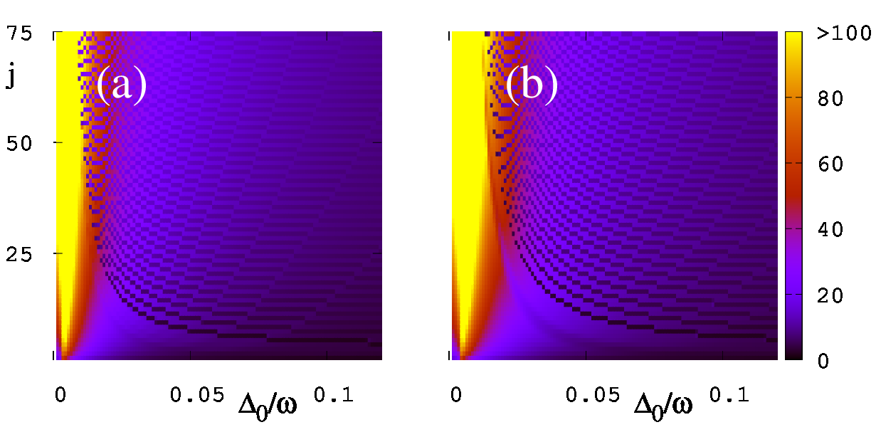
Figure 1: Participation ratio $\xi$ of eigenstates $\psi_{j}$ of RWA Hamiltonian (4) as a function of rescaled resonance detuning $\Delta_{0}/\omega$ and eigenstate index $j$ which counts eigenenergies in their monotonically increasing order; here $f=5^{-\frac{3}{2}}\simeq 0.0894$, $g=0.04$ and $g=0.08$ in left $(a)$ and right $(b)$ panels respectively; $xi$ values are shown by color with the corresponding color bar. Here and in all other Figures we use dimensionless units explained in the text.

The eigenstates $\psi_{j}$ of RWA Hamiltonian (4) are determined by the equation $\hat{H}_{r}\psi_{j}(n,\sigma_{z})=E_{j}\psi_{j}(n,\sigma_{z})$. We order the index $j$ in such a way that the energy eigenvalues $E_{j}$ are monotonically growing with $j$.

The numerical computation of eigenstates $\psi_{j}$ is done by a direct matrix diagonalization with a truncated basis of oscillator eigenstates with $0\leq n\leq N-1$. We checked that the value of $N=700$ is sufficient to have stable eigenstates with $j<100$ so thus the following numerical results are obtained with this $N$ value. Thus, with qubit, in total we have $2N=1400$ states. We also use the same $N$ to obtain the time evolution of initial Hamiltonian (1). The time evolution is obtained by the Trotter decomposition with the time step $\Delta=0.005$ (the results are not sensitive to further decrease of the time step).

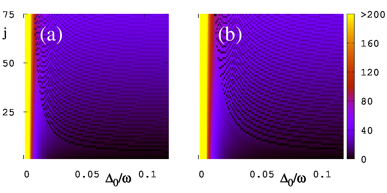
Figure 2: Average oscillator number $<n>$ for eigenstates of Hamiltonian (4) shown by color for the parameters of Fig. 1 with $g=0.04$ and $g=0.08$ in left $(a)$ and right $(b)$ panels respectively.

We characterize the eigenstates of $H$ (1) and $H_{r}$ (4) by their participation ratio (PR) defined as $\xi_{j}=\sum_{n\sigma_{z}}|\psi_{j}(n,\sigma_{z})|^{2}/\sum_{n\sigma_{z}}|\psi_{j}(n,\sigma_{z})|^{4}$. Here $\psi_{j}(n,\sigma_{z})$ represents the eigenfunction expansion in the eigenbasis at $g=0$. Thus $\xi_{j}$ gives an effective number of decoupled states (at $g=0$) contributing to a given eigenstate at $g>0$. For a given eigenstate we also compute the average photon number $\langle\psi_{j}|\hat{n}|\psi_{j}\rangle=\langle n\rangle$ and the average qubit (spin) polarization $<\sigma_{z}>$.

The dependencies of $\xi$, $<n>$, $<\sigma_{z}>$, for eigenstates $\psi_{j}$ of Hamiltonian (4), on $j$ and rescaled detuning frequency $\Delta_{0}/\omega$ are shown in Figs. 1, 2, 3 respectively. These results show that in a vicinity of resonance many oscillator states are populated that is rather natural. The polarization dependence is more tricky being close to zero in direct resonance vicinity and becoming mainly negative with detuning increase and later followed by a polarization change from positive to negative. We will return to the discussion of these properties in next Sections.

According to the analytical result obtained in the RWA frame in refereeref1 for the case of exact resonance the Floquet eigenstates become fully delocalized over all oscillator states (being non-normalizable) for $f\geq g$. Our numerical results confirm this delocalization both for non-RWA case of Hamiltonian (1) and for RWA case of Hamiltonian (4). These results are presented in Appendix Fig. 12.

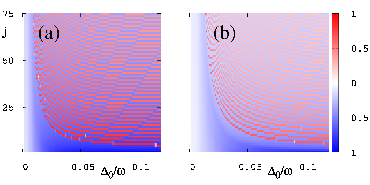
Figure 3: Average spin $<\sigma_{z}>$ for eigenstates of Hamiltonian (4) shown by color for the parameters of Fig. 1 with $g=0.04$ and $g=0.08$ in left $(a)$ and right $(b)$ panels respectively.

III Analytical results

For analytical analysis of driven JCM we perform in (4) an additional transformation using the replacement $\hat{a}=\hat{b}-\frac{f}{2\Delta_{0}}$ that gives us a transformed Hamiltonian

$$\hat{H_{rt}}=\Delta_{0}\hat{n}_{b}+\frac{\Delta_{\Omega}}{2}\hat{\sigma}_{z}+g\omega_{0}\left(\hat{b}\hat{\sigma}_{+}+\hat{b}^{\dagger}\hat{\sigma}_{-}\right)+B_{x}\hat{\sigma}_{x}+K\;.$$ (5)

This shows an appearance of an effective field $B_{x}={fg\omega_{0}}/({2\Delta_{0}})$ and a constant term $K={f^{2}}/({4\Delta_{0}})$. The interesting feature of the expression (5) is that even for small $g$ values we obtain an effective JCM with a strong effective values of effective coupling constant $g_{eff}=g\omega_{0}/\Delta_{0}\gg g$ at small resonance detunings $\Delta_{0}\ll\omega_{0}$.

It is important to note that in (5) we effectively obtain the JCM with a strong coupling $g_{eff}>1$ between oscillator and spin. In fact it is known that without RWA the original JCM at strong coupling is characterized by a chaotic dynamics for the corresponding classical equations of motion zaslavsky ; milonni . In the quantum case such a chaotic dynamics leads to quantum chaos for several spins interacting with a resonator with the level spacing statistics as for random matrix theory graham . Thus the monochromatically driven JCM can be used for investigations of many-spin quantum chaos induced by an effective strong coupling to a resonator.

On the other hand, the semiclassical version of Eq.(4) can be written in spin 1/2 basis as

$$H_{sc} = \frac{p^{2}}{2}+\frac{\Delta_{0}^{2}x^{2}}{2}+f\sqrt{\frac{\Delta_{0}}{2}}x+$$

$$+ \left(\begin{array}[]{cc}\frac{1}{2}\Delta_{\Omega}&\sqrt{\frac{\Delta_{0}g^{2}\omega_{0}^{2}}{2}}\left(x+\frac{ip}{\Delta_{0}}\right)\\ \sqrt{\frac{\Delta_{0}g^{2}\omega_{0}^{2}}{2}}\left(x-\frac{ip}{\Delta_{0}}\right)&-\frac{1}{2}\Delta_{\Omega}\\ \end{array}\right)$$

which can be diagonalized, with the corresponding solution:

$$h = h_{0}+f\sqrt{\frac{\Delta_{0}}{2}}x\pm\sqrt{\frac{g^{2}\omega_{0}^{2}}{\Delta_{0}}h_{0}+\frac{\Delta_{\Omega}^{2}}{4}}$$ (9)

$$h_{0} = \frac{p^{2}}{2}+\frac{\Delta_{0}^{2}x^{2}}{2}\;.$$

Here $(x.p)$ are classical coordinate and momentum of oscillator which mass is taken to be unity $m=1$. The linear term in $x$ in (9) simply gives a shift of oscillator center position.

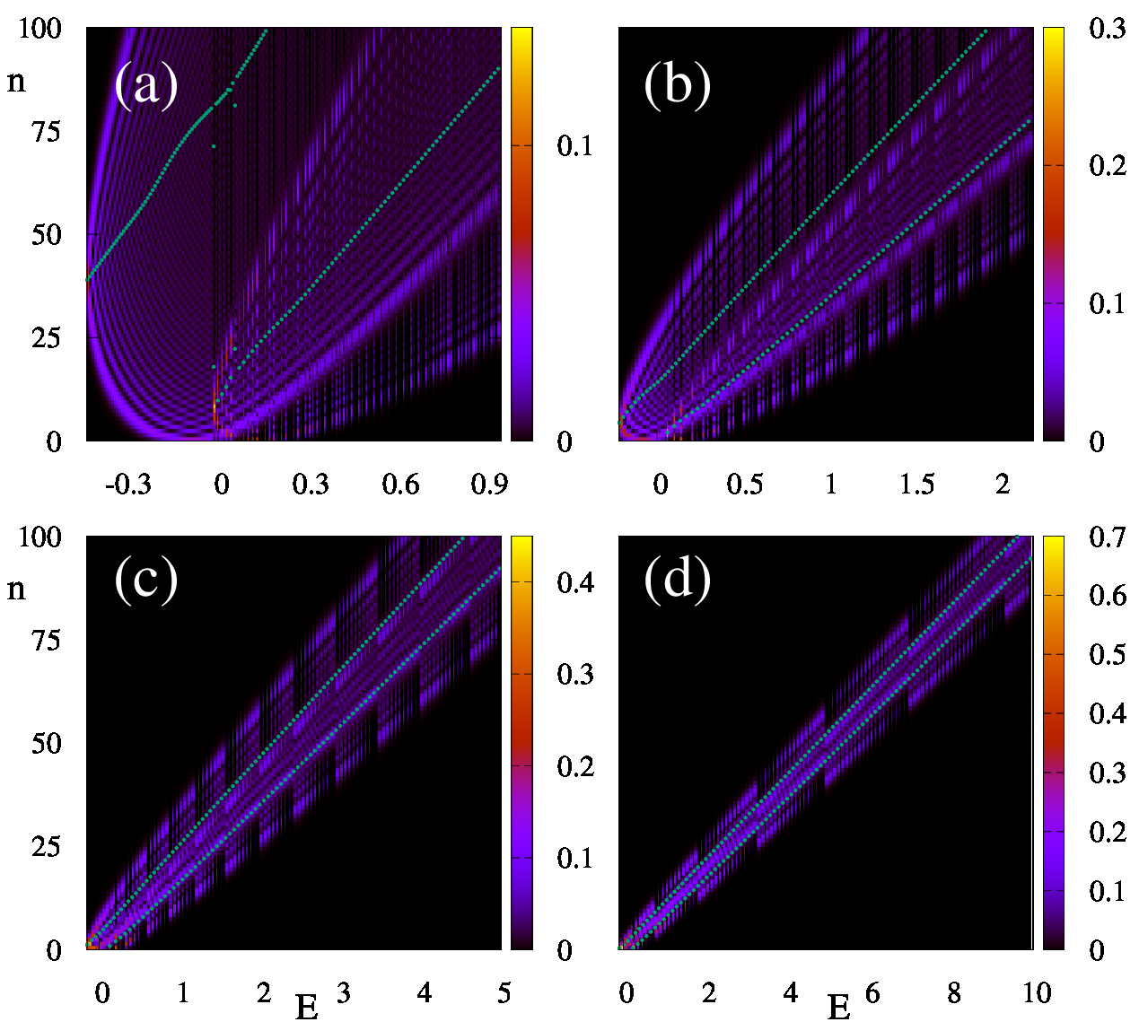
Figure 4: Probability distribution $P(n)=|\langle n|\psi_{j}\rangle|^{2}$ (tracing out spin space) of $j^{th}$ eigenstate of (4) ordered by increasing energy $H|\psi_{j}\rangle=E_{j}|\psi_{j}\rangle$. The values of parameters are $g=0.04$, and $\Delta_{0}=\omega_{0}-\omega=0.01,0.025,0.05,0.1$ in panels (a), (b), (c) and (d) respectively. The green dotted curves show the mean value $\langle n\rangle$ of the corresponding eigenstate $\psi_{j}$. The color map goes from black at 0 to yellow at maximum value given by $0.14$ for $(a)$, $0.3$ for $(b)$, $0.45$ for $(c)$ and $0.7$ for $(d)$.

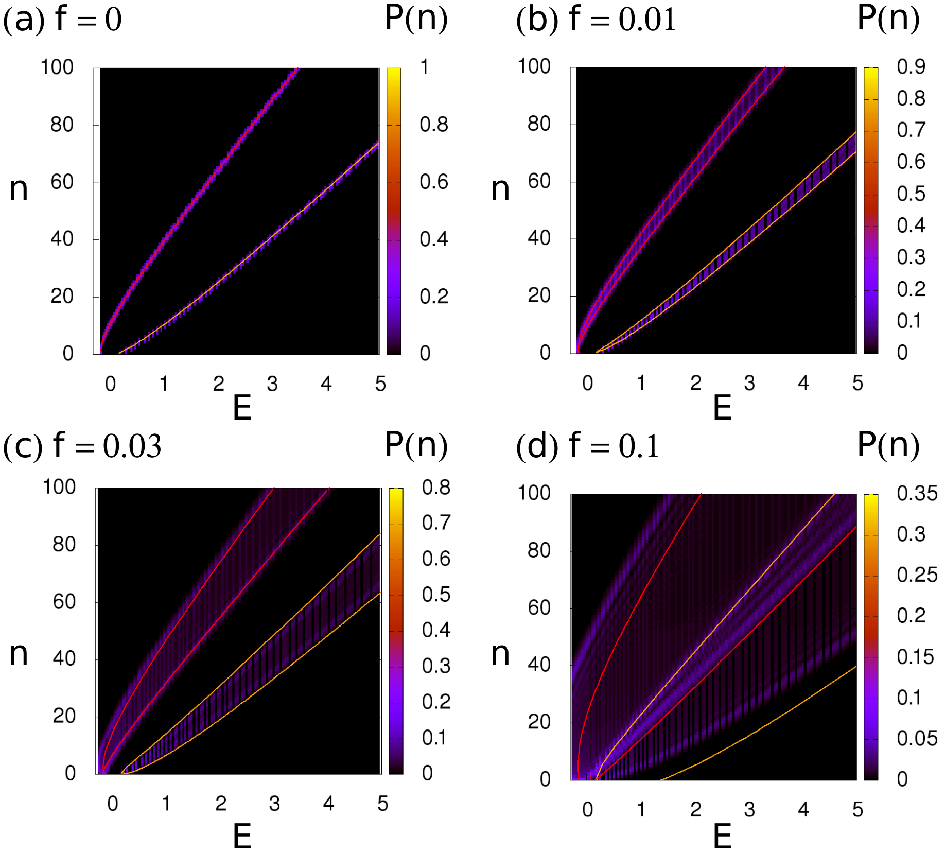
Figure 5: Probability distribution $P(n)$ of the eigenstates of $\psi$ Eq. (4) ordered by increasing energy ${\hat{H}}\psi=E\psi$ for different values of the driving force $f$. The other parameters of the Hamiltonian are set to $\Delta_{\Omega}=0.25$, $\Delta_{0}=0.05$, $g\omega_{0}=0.15$. The red/orange lines show the semi-classical estimate expressions for the positions of $P(n)$ maxima for the two-spin eigenstates of the semi-classical hamiltonian given by Eqs. (11,12). The semi-classical curves are in a good agreement with the data from quantum wavefunctions and give a physical interpretation for the position of the maxima of $P(n)$.

The above expressions also allow to obtain the semiclassical expression for the average spin polarization being

$$\langle\sigma_{z}\rangle=\pm\left(1+4g^{2}\omega_{0}^{2}\langle n\rangle/\Delta_{\Omega}^{2}\right)^{-\frac{1}{2}}.$$ (10)

The semiclassical theoretical expressions (9) gives us the dependence of RWA energy $h$ on unperturbed energy $h_{0}$ which we compare with the results of numerical simulations in the next Section. We also compare the theoretical spin polarization (10) with the numerical results.

IV Numerical results

The eigenstates of Hamiltonian (4) are obtained by a direct numerical matrix diagonalization with the numerical parameter described above. The eigenstate probability distribution of $\psi_{j}$ is shown in Fig. 4 as a function of oscillator number $n$ and eigenenergy $E=E_{j}$. We clearly see the presence of two branches corresponding to two spin polarization. The mean values of $\langle n\rangle$ are shown by green dotted curves marking the average dependence $n(E)$ for each branch. In Appendix Fig. 13, for comparison we show the same characteristics as in Fig. 4 but for eigenstates of transformed Hamiltonian (5). We obtain a good agreement between the eigenstates of these two Hamiltonian confirming the validity of the analytical transformation from one to another. At the same time at very small resonance detunings $\Delta_{0}=0.01$ there are certain differences between these two representations which we attribute to high order corrections in a resonance vicinity.

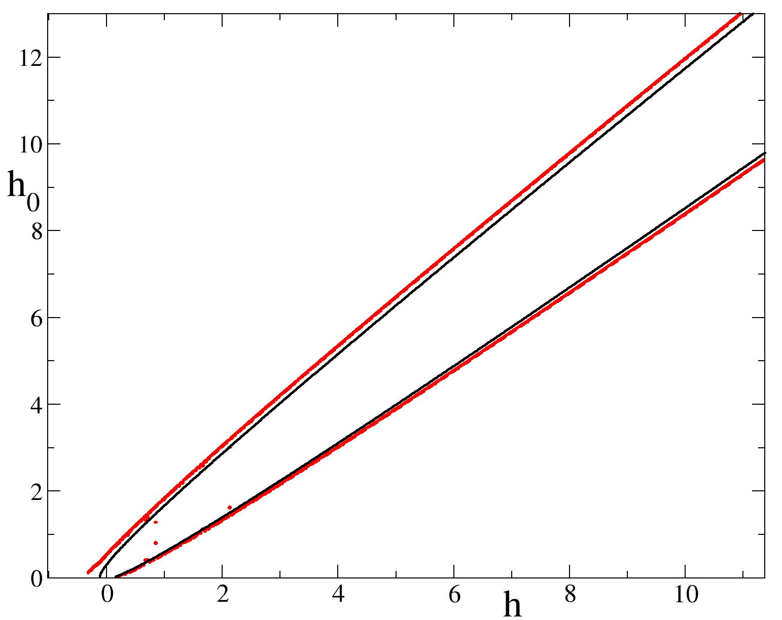
Figure 6: Quantum harmonic oscillator Hamiltonian $h_{0}$ vs. $h$ from (9). Two branches of (9) for $f=0$ are shown in black line, while mean values of $\langle h_{0}\rangle$ as a function of $\langle h\rangle$ obtained from the numerical diagonalization of Hamiltonian (4) are shown by red (gray) dots. The parameter values are $g=0.04$, $\omega=1$, $\omega_{0}=0.975$, $\Omega=1.2$, $g=0.04$ and $f=\hbar\lambda\sqrt{n_{p}}$ with $\lambda=0.02$ and $n_{p}=20$ which are the same as in panel (b) of Fig 4.

Averaging the semi-classical Hamiltonian over an oscillation period, we find the mean oscillator quantum number $\langle n\rangle=h_{0}/\Delta_{0}$ as function of the eigenstate energy $E=h$ as the positive solutions of the equation:

$$E =\Delta_{0}\langle n\rangle\pm\sqrt{g^{2}\omega_{0}^{2}\langle n\rangle+\frac{\Delta_{\Omega}^{2}}{4}}$$ (11)

the two possible signs correspond to the two spin-eigenstates of Eq. (III). As can be seen from Fig. (4), the probability $P(n)$ is in general not peaked at its average value $\langle n\rangle$, instead (for a fixed eigenstate) $P(n)$ is non zero for n in a range $(n_{min},n_{max})$ with maxima at both $n_{min}$ and $n_{max}$. The position of the maxima can be understood from the following argument. For simplicity we neglect the change in the Zeeman-like energy term of Eq. (III), in the conservation of energy for semiclassical motion is then $h\simeq h_{0}+f\sqrt{\frac{\Delta_{0}}{2}}x(t)$ where the position $x(t)$ follows an oscillation with amplitude $\sqrt{2\langle n\rangle/\Delta_{0}}$. The change in potential energy $f\sqrt{\frac{\Delta_{0}}{2}}x(t)$ is approximately compensated by a change of $h_{0}=\Delta_{0}n$. The most likely value of $h_{0}$ correspond to inflection points of the trajectory giving the estimate:

$$n_{max,min} =\langle n\rangle\pm\frac{f\sqrt{\langle n\rangle}}{\Delta_{0}}$$ (12)

This estimation is compared with numerical data on Fig. (5) for different strengths of the force $f$ showing a good agreement with the roating-wave Hamiltonian wavefunctions. It is interesting that these simple semi-classical arguments allow to understand some nontrivial wavefunctions properties of the driven Jaynes-Cummings model wavefunctions.

The comparison between the numerical results obtained from the eigenstates of Hamiltonian (4) and the semiclassical theory of (9) is also shown in Fig. 6. It shows a good agreement between the theory and numerical results.

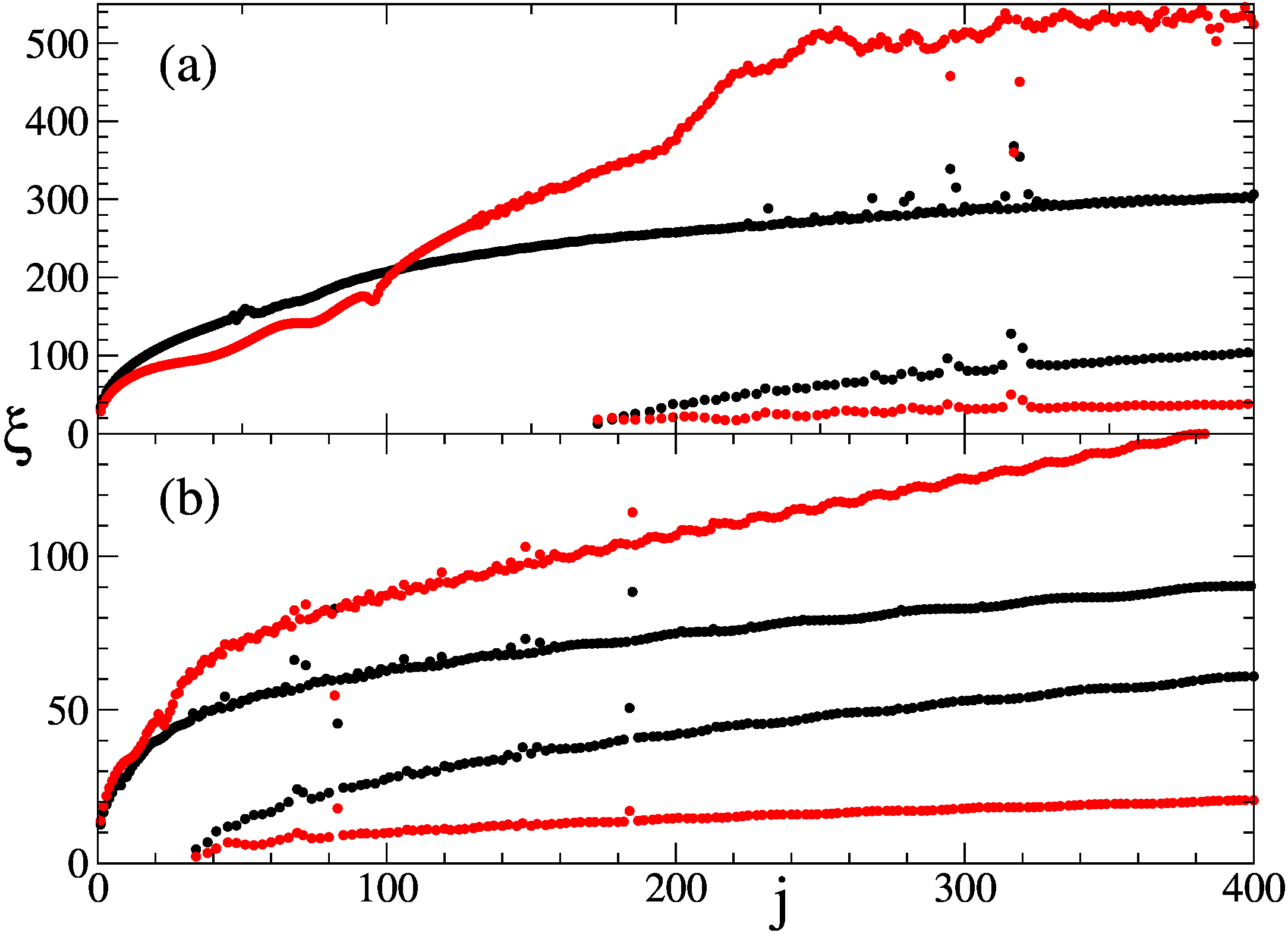
Figure 7: Participation ratio $\xi$ of eigenstates of Hamiltonian $H$ (4) as a function of eigenstate index $j^{\text{th}}$. Here, the values $\xi$, computed for eigenstates of both $\hat{n}$ and $\hat{\sigma}_{z}$, are shown by black circles. Floquet states (ordered by increasing mean value of $\langle H\rangle$ averaged in a period) of (1) are shown with red (gray) circles. Here we have values $\omega_{0}=0.99$ ($\Delta_{0}=0.01$) and $\omega_{0}=0.975$ ($\Delta_{0}=0.025$) in top (a) and bottom (b) panels respectively with $g=0.04$, $\omega=1$, $\Omega=1.2$ and $f=\hbar\lambda\sqrt{n_{p}}$ with $\lambda=0.02$ and $n_{p}=20$. These values are the same as in panels (a) and (b) of Fig 4 respectively.

The validity of the semiclassical description (9) is confirmed by the numerical results presented in Fig. 6 showing the dependence $h_{0}(h)$ for two spin (or qubit) projections. Indeed, there is a good agreement between the numerical results obtained for the Hamiltonian (4).

It is important to compare the numerical results obtained in the RWA of (4) with the those obtained from the Floquet eigenstates of (1). The index $j$ for Floquet eigenstates is defined for increasing value of $\langle H\rangle$ averaged over a period. We present the comparison for the participation ratio $\xi$ shown in Fig. 7. It shows a qualitative agreement between the Floquet results of (1) and those obtained for the RWA Hamiltonian (4). However, the quantitative agreement is absent showing that $\xi$ values from RWA are by a factor 2 different from Floquet values of (1). We attribute this difference for the fact that the results are obtained in a close vicinity to the resonance with $\omega_{0}$ being very close to the driven frequency $\omega$. In such a case next order corrections beyond RWA can produce additional frequency shifts providing rescaling of an effecting value of frequency detuning that would notably affect the values of participation ration $\xi$ of eigenstates. We note that the difference between RWA an non-RWA cases in a resonance vicinity was also pointed in refereeref2 even if the regime of strong oscillator excitation was not analyzed in detail there.

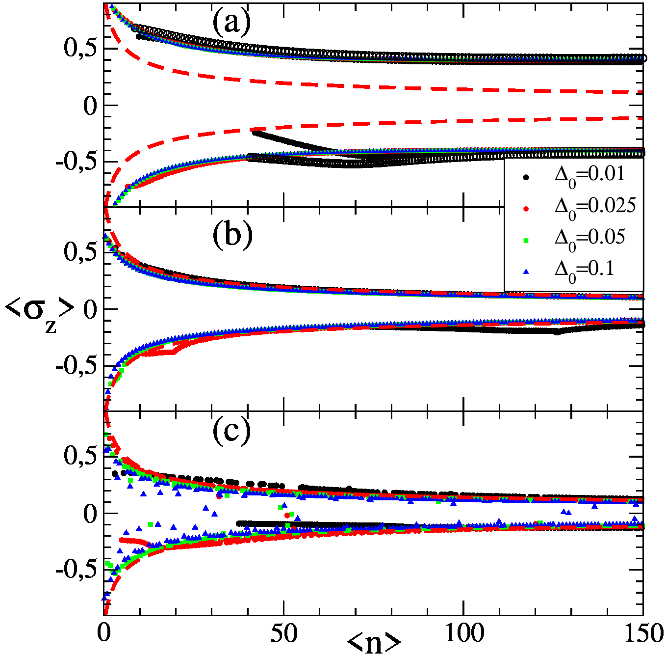
Figure 8: Average spin polarization as a function of mean oscillator number ($\langle\sigma_{z}\rangle$ vs. $\langle n\rangle$) for eigenstates of $H$. Top (a), middle (b) and bottom (c) panels show the cases of Hamiltonian (1), (4) and 5) respectively. Parameter values are $g=0.04$, $\omega=1$, $\Omega=1.2$ and $f=\hbar\lambda\sqrt{n_{p}}$ with $\lambda=0.02$ and $n_{p}=20$, with $\Delta_{0}=0.01,0.025,0.05,0.1$ in black circles, red (gray) circles, green squares and blue triangles respectively. The semiclassical theoretical dependence (10) curve given by is shown by red dashed red (gray) curve for $\Delta_{0}=0.025$.

According to the above argument the agreement between data obtained from (1), (4), (5) should become better with the increase of resonance detuning $\Delta_{0}$. We check this determining the dependence of average spin polarization $\langle\sigma_{z}\rangle$ on average quantum number of oscillator $\langle n\rangle$ as it is presented in Fig. 8. The comparison shows that the semiclassical theory (10) well describes the numerical results of RWA from Hamiltonians of (4), (5). However, there is a notable deviations between the theory and RWA numerical results from the Floquet results. At the same time, the results presented in Appendix Fig 14, 15 show that the agreement between the Floquet results of (1) and the RWA results of (4) becomes better with in increase of resonance detuning $\Delta_{0}$ and decrease of coupling strength $g$. This confirms our argument that the difference between the Floquet and RWA results are related to higher order corrections related to coupling $g$ which play a more significant role in a close vicinity to the resonance.

Figure 9: Quantum harmonic oscillator Hamiltonian $h_{0}$ vs. $h$ for Floquet eigenstates $|\Psi_{j}(t=0)\rangle$. $h_{0}=\langle\Psi_{j}(t=0)|\hbar\omega\hat{n}|\Psi_{j}(t=0)\rangle$ and $h=\langle\Psi_{j}(t=0)|\hat{H}|\Psi_{j}(t=0)\rangle$ with $\hat{H}$ of Eq.1 Parameter values are $g=0.04$, $\omega=1$, $\omega_{0}=0.975$, $\Omega=1.2$ and $f=5^{-\frac{3}{2}}$ which are the same than panel $(b)$ of Fig 4. Red and green circles represent the Floquet states shown in Fig 10 in top ($(a)$ and $(b)$) and bottom ($(c)$ and $(d)$) panels.

In Fig. 9 we show the two branch dependence, corresponding to two spin polarizations, of quantities $h_{0},h$ described above. $h_{0}$ and $h$ of Fig. 9 are computed for Floquet eigenstates $|\Psi_{j}(t=0)\rangle$ valued in initial state $t=0$ as $h_{0}=\langle\Psi_{j}(t=0)|\hbar\omega\hat{n}|\Psi_{j}(t=0)\rangle$ and $h=\langle\Psi_{j}(t=0)|\hat{H}|\Psi_{j}(t=0)\rangle$ where $\hat{H}$ is defined in Eq.1. We also mark with red and green circles there the values of $h_{0},h$ obtained for two given Floquet states described in the next Section. The presence of two branches obtained from the developed semiclassical description corresponds to the bistability behavior found in zsprl for the evolution of Hamiltonian (1) in presence of dissipation.

V Husimi function evolution

In this Section we consider the phase space representation in the plane coordinate and momentum $(q,p)$ of certain Floquet eigenmodes of (1) and the time evolution of certain initial coherent states. The phase space representation of quantum states is done with the Husimi function which gives the Wigner function smoothed on a scale of Planck constant (see e.g. husimi1 ; husimi2 ). The smoothing is done with the oscillator coherent state corresponding to a Gaussian wave packet that is localized in the classical phase space around a point $(q_{0},p_{0})$ in the phase space. The smoothing is given by the relation $\langle x|\varphi(p_{0},q_{0}){>}=Ae^{-(x-q_{0})^{2}/2+\frac{i}{\hbar}p_{0}(x-q_{0})},$ with wave packet the same widths coordinate and momentum $\Delta p=\Delta q=1/2$, and with the normalization constant $A$ (see more details in husimi1 ; husimi2 ). Then the Husimi function probability $\rho_{H}$ in the phase space $(q_{0},p_{0})$ is given by the relation $\rho_{H}(p_{0},\theta_{0})=|{<}\varphi(p_{0},\theta_{0})\,|\,\psi{>}|^{2}$. We construct the Husimi function for up and down $\sigma_{z}$-spin components of the total wavefunction.

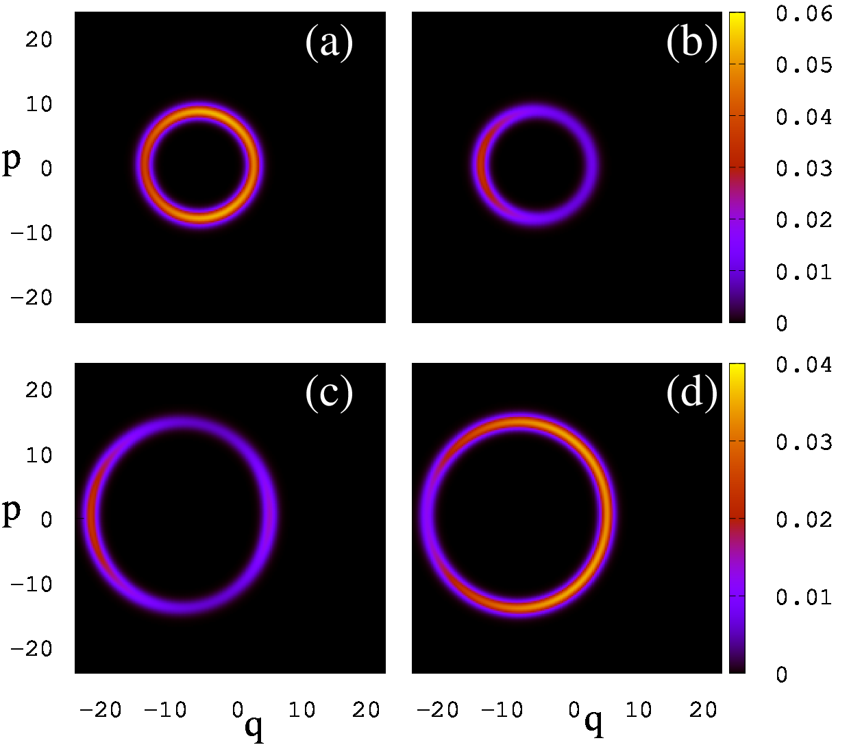
Figure 10: Husimi representation in phase space of two Floquet states with $t=0$. Left ($(a)$ and $(c)$) and right ($(b)$ and $(d)$) panels show the $\Pi_{0}\equiv|0\rangle\langle 0|$ and $\Pi_{1}=|1\rangle\langle 1|$ projection in $\hat{\sigma}_{z}$ respectively of two Floquet states. The parameter values are the same as in Fig 9, where both Floquet modes are shown in ($h,h_{0}$) plane with color circles: red for $(a)$ and $(b)$ ($h\simeq 11.64,h_{0}\simeq 8.99$) and green for $(c)$ and $(d)$ ($h\simeq 129.13,h_{0}\simeq 65.0$). The color map goes from black at 0 to yellow at maximum value given by 0.06 for $(a)$ and $(b)$, and 0.04 for $(c)$ and $(d)$.

In Fig. 10 we present the Husimi functions for spin up and down for a typical Floquet eigenstate with $\lambda=0.02$ and system parameters given in Fig. 9. The results clearly show that the eigenstate have double contribution of small and large oscillator numbers $n$ with a small circle in top panels and large circle in bottom panels respectively (this doublet structure is present for both spin projections shown in left and right panels). This example shows that all phases of a circle in $(q,p)$ plane are present but the distribution over the phases is inhomogeneous. The two sizes of the circle corresponds to the two semiclassical branches appearing in (9).

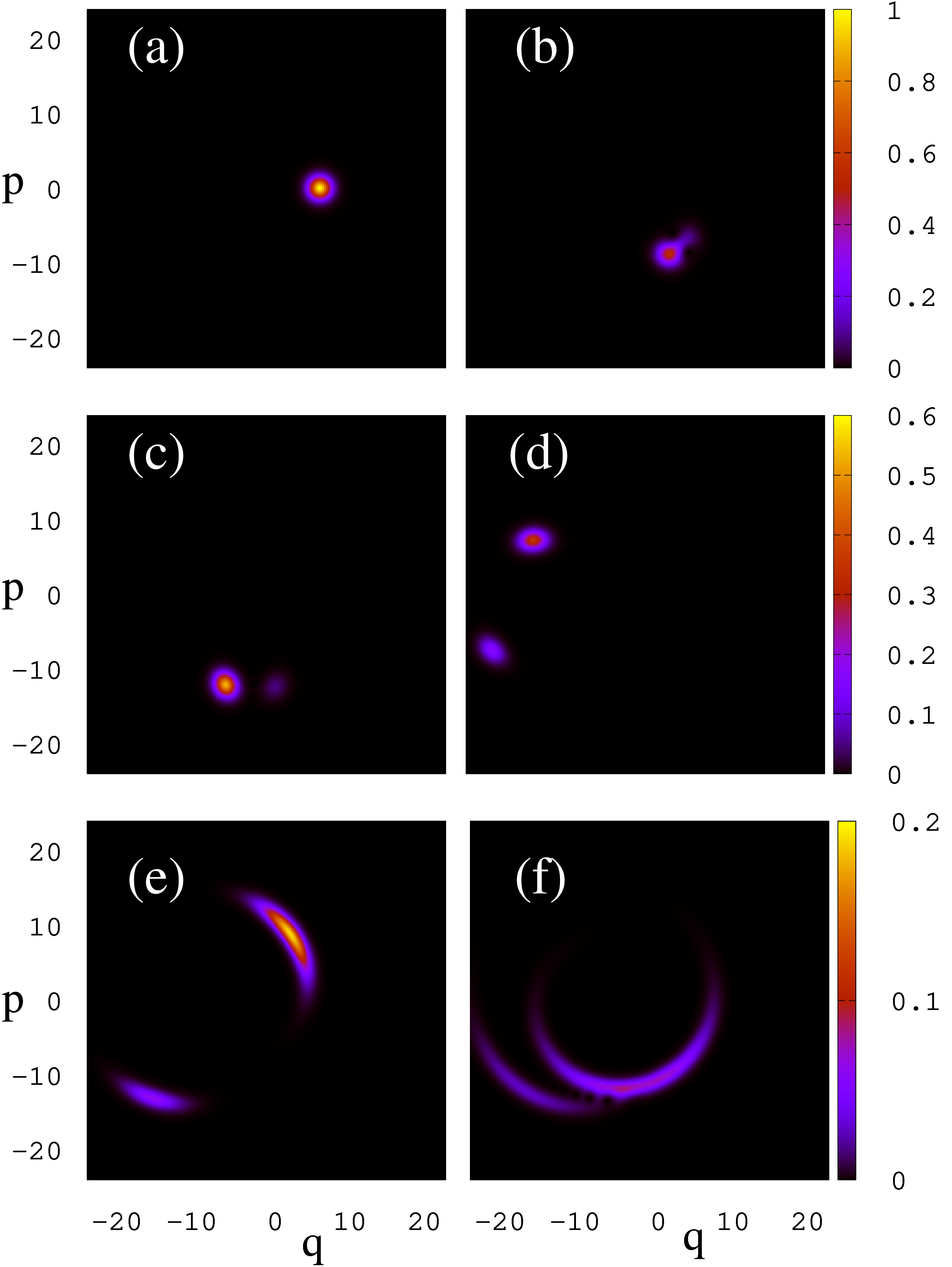
Figure 11: Husimi representation in phase space the evolution of a coherent state. Initial state is given by a coherent state centered at $(q_{0},p_{0})=(5,0)$ and spin projection $\Pi_{0}=|0\rangle\langle 0|$ shown in panel (a). Time evolution of $\Pi_{0}$ projection is also shown for times $\omega t/2\pi=10,20$, $50$ and $400$, $1000$ in $(b),(c)$, $(d)$ and $(e),(f)$ panels respectively. Parameter values are $g=0.04$, $\omega=1$, $\omega_{0}=0.975$, $\Omega=1.2$ and $f=5^{-\frac{3}{2}}$ which are the same as in panel $(b)$ of Fig 4. The videos of time evolution are available at suppmat .

The snapshots of time evolution of the Husimi function of an initial coherent state are shown in Fig. 11. At large times the localized coherent state, shown in videos available at suppmat , spreads over the whole circle corresponding to a given oscillator number that is in agreement with the Floquet eigenstate structure shown in Fig. 10 where the probability is distributed over all circle phases even if the distribution is inhomogeneous. The videos are obtained from the Floquet system (1) and from the RWA Hamiltonian (2). The evolution in both cases is similar but not exactly the same. More details about videos are given in Appendix. The time of such a spreading $t_{sp}$ over the whole circle is rather long with $\omega t_{sp}/2\pi\approx 1000$.

We attribute it to the nonlinear energy dispersion correction appearing in driven JCM due to coupling between the spin and oscillator with $\delta\omega=\delta E_{n}\approx\pm g\omega_{0}\sqrt{n/\Delta_{0}}$ (see (9)). In fact this nonlinear dependence of energy shift $\delta E_{n}$ on level number $n$ (or classical action) should lead to appearance of a nonlinear resonance with the driving frequency $\omega$. In principle, such a resonance can be treated in the pendulum approximation of an isolated resonance as described in chirikov . Due to two spin orientations we will have two resonances corresponding to spin up and down branches discussed above. Thus there should exist a tunneling between this two branches with a certain tunneling time $\tau$. The results presented in zsprl (see Fig.5 there) show that the tunneling times $\tau$, expressed in number of driving periods, can be rather long with $\tau\sim 10^{3}-10^{4}$. We expect that the further development of the nonlinear resonance theory can allow to understand the mechanism of this long time tunneling process and obtain the estimates for its dependence on system parameters. However, this requires to perform additional investigations going beyond the studies presented here. In the language of the Floquet eigenvalues the tunneling process should be related to appearing of very tiny splittings between Floquet eigenenergies $\epsilon_{j}$ in (3).

VI Discussion

In this work we analyzed the JCM behavior under a monochromatic driving. Our analytical and numerical results show that the system can be effectively reduced to a modified JCM with a strong coupling between photons and qubit. The obtained results allow to understand the process of two branches of excitation of many photons induced by the driving in presence of nonlinear frequency dispersion induced by coupling between photons and qubit. The obtained analytical semiclassical formula gives a good description of obtained numerical results. However, in a very close vicinity of the resonance between frequencies of oscillator and monochromatic driving there appear certain deviations which we attribute to high order corrections to RWA approach which become important in close resonance vicinity. The obtained results still keep certain open questions on properties on the driven JCM, in particular the question about the physical estimates of long tunneling times between two branches corresponding to up and down qubit polarization, which are also present in the dissipative case zsprl .

Here we analyzed the case of unitary driven JCM system. In experiments the dissipative effects start to play and important role. However, at a weak dissipation the results obtained for the unitary evolution will allow to have a better understanding of dissipative quantum behavior. Thus our semiclassical theory for the unitary evolution explains the appearance of bistability in the dissipative case zsprl .

Since the JCM is the fundamental system of quantum optics we hope that the reach properties of driven JCM will attract interest of experimental groups working with superconducting qubits and other systems of quantum optics.

*

Appendix A

Here we present supplementary figures complementing the main text of the paper.

In Fig. 12 we show that for the case of exact resonance $\omega=\omega_{0}$ the probability is rapidly transferred to highest oscillator levels, available for a given computational basis, for $f\geq g$ while for $f<g$ the probability of high levels remains very small. This numerical result is obtained both in RWA frame and without RWA for the Hamiltonian (1). Thus for $f\geq g$ the Floquet states are delocalized and non-nonrmalizable. This result is in agreement with the analytical result obtained within RWA in refereeref1 . Fig. 13 shows properties of eigenstates of Hamiltonian (5) fog parameters of Fog. 4.

Figure 12: Time evolution of total probability $P_{b}$ at 20 highest oscillator levels (with both spin components) for numerical simulations with basis of $1000$ oscillator states. At the initial state the oscillator is at level $n=1$ and the spin is at its down-component. Parameter values are $\omega=\omega_{0}=1$, $\Omega=1$, $g=0.04$ and $f=g/2$ (black curves), $f=g$ (red (gray) curves), $f=2g$ (blue (dark gray) curves), where the dashed curves represent the computations within RWA frame and full curves are for results without RWA for the Hamiltonian (1). Black curves are saturated at the level of $P_{b}\approx 10^{-24}$ at $\omega t=30$; at the level $P_{b}\approx 10^{-16}$ the blue (dark gray) curves are located at $\omega t\approx 4$ and the red (gray) curves are located at $\omega t\approx 7.5$.

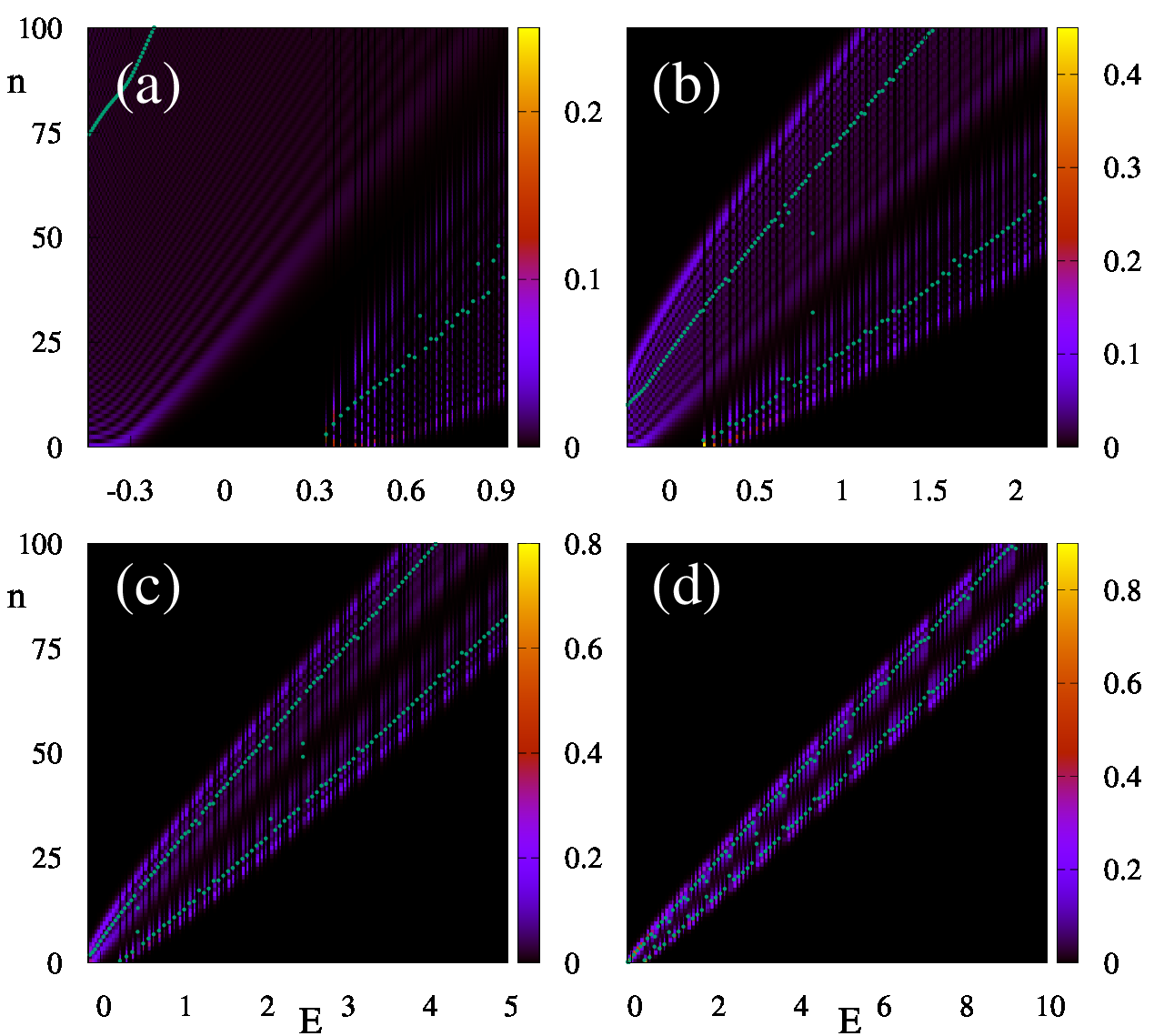
Figure 13: Same quantities and parameters as in Fig. 4 but the eigenstates are obtained from the numerical diagonalization of transformed Hamiltonian (5). The color map goes from black at 0 to yellow at maximum value given by $0.25$ for $(a)$, $0.45$ for $(b)$, $0.8$ for $(c)$ and $0.9$ for $(d)$.

Fig. 14 and Fig. 15 show the average spin polarization as a function of the mean oscillator number ($\langle\sigma_{z}\rangle$ vs. $\langle n\rangle$) for eigenstates of the Hamiltonian of Eq. 1 (black circles) and Eq 4 (red circles) with $\Delta_{0}=0.01$ and $\Delta_{0}=0.025$ respectively. Each panel on both figures represent a different value of $g$: $0.0025$ $(a)$, $0.005$ $(b)$, $0.0088$ $(c)$, $0.0138$ $(d)$, $0.0375$ $(e)$ and $0.05$ $(f)$.

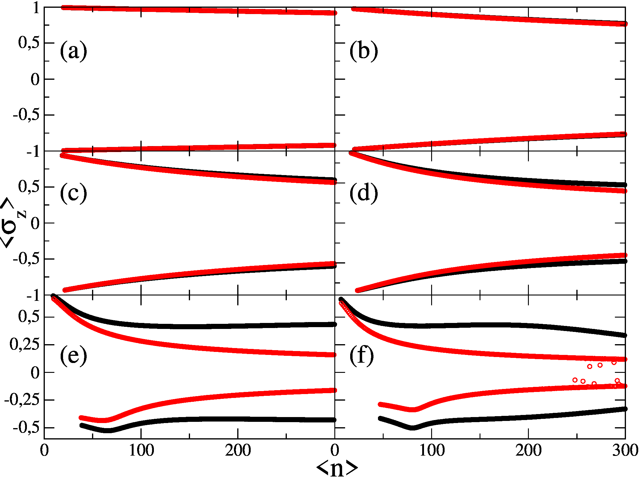
Figure 14: $\langle\sigma_{z}\rangle$ vs. $\langle n\rangle$ for eigenstates of $H$ with $\Delta_{0}=0.01$ and different values of $g$. Black and red (gray) circles show the cases of Hamiltonian of Eq. 1 and Eq. 4 respectively. Parameter values are $\omega=1$, $\Omega=1.2$ and $f=5^{-\frac{3}{2}}$ with a different value of $g$ en each panel: $0.0025$ $(a)$, 0.005 $(b)$, 0.0088 $(c)$, 0.0138 $(d)$, 0.0375 $(e)$ and 0.05 $(f)$.

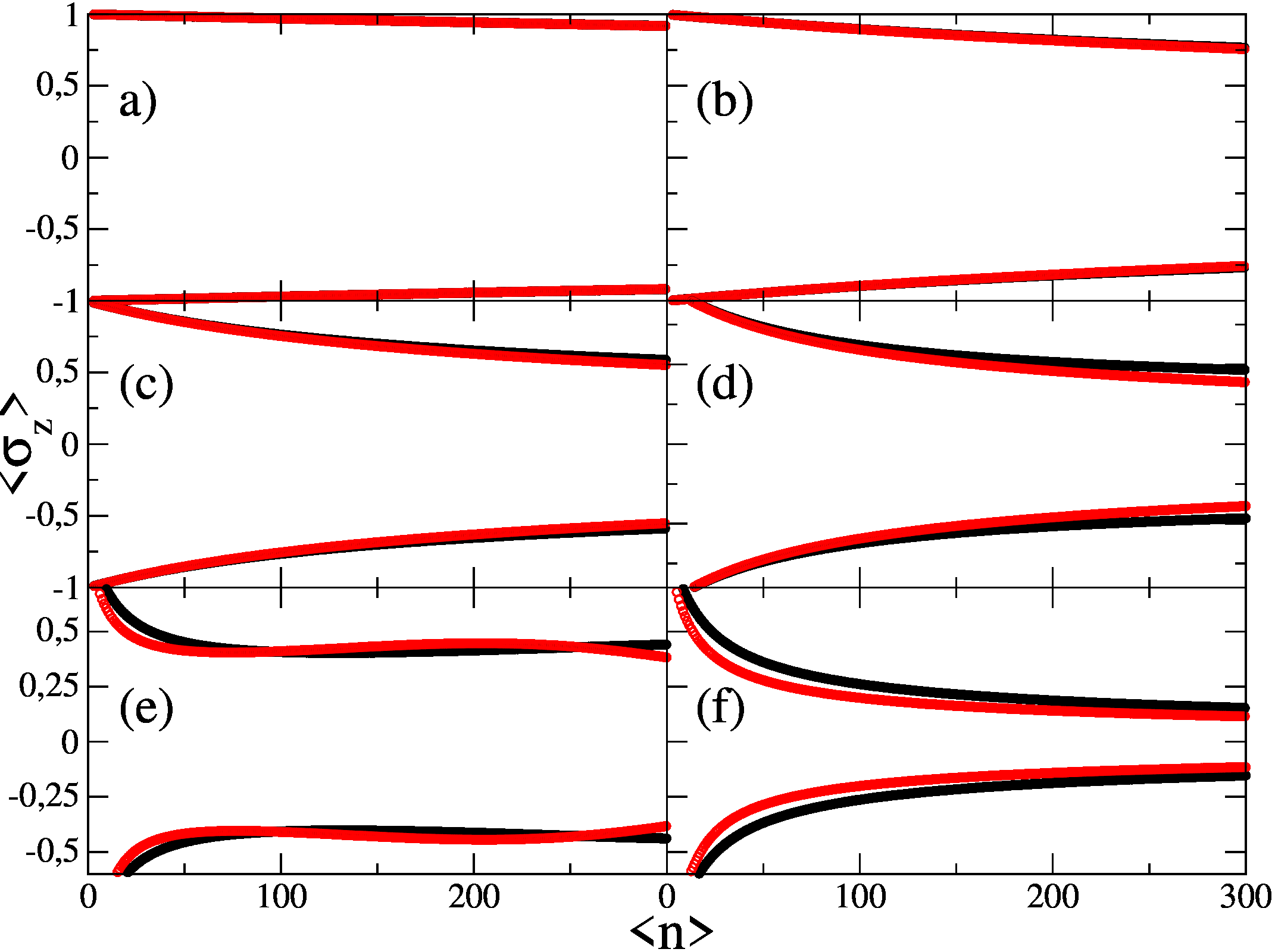
Figure 15: $\langle\sigma_{z}\rangle$ vs. $\langle n\rangle$ for eigenstates of $H$ with $\Delta_{0}=0.025$. Black and red (gray) circles show the cases of Hamiltonian of Eq. 1 and Eq. 4 respectively. Parameter values are the same as in Fig. 14 but with $\Delta_{0}=0.025$. Each panel represent a different value of $g=0.0025$ $(a)$, 0.005 $(b)$, 0.0088 $(c)$, 0.0138 $(d)$, 0.0375 $(e)$ and 0.05 $(f)$.

Videos in suppmat present the time evolution of Husimi function for parameters of Fig. 11; videohusimi1.mp4 is obtained from the time evolution given by Floquet system (1) and videohusimi2.mp4 is obtained from the RWA Hamiltonian (2). Initial state is given by a coherent state centered at $(q_{0},p_{0})=(5,0)$ with a spin projection in $|0\rangle$. Parameter values are $g=0.04$, $\omega=1$, $\omega_{0}=0.975$, $\Omega=1.2$ and $f=\hbar\lambda\sqrt{n_{p}}$ with $\lambda=0.02$ and $n_{p}=20$.

References

- (1) E.T. Jaynes, and F.W. Cummings, Comparison of quantum and semiclassical radiation theories with application to the beam maser”, Proc. IEEE. 51(1), 89 (1963).
- (2) J.J. Sanchez-Mondragon, N.B. Narozhny, and J.H. Eberly, Theory of spontaneous-emission line shape in an ideal cavity, Phys. Rev. Lett. 51m 550 (1983).
- (3) L. Allen and J.H. Eberly, Optical resonance and two-level atoms, Dover Publs. Inc., New York (1987).
- (4) M.O. Scully, and M.S. Zubairy, Quantum optics, (Cambridge University Press, Cambridge, England, 1997).
- (5) G. Rempe, H. Walther and N. Klein, Observation of quantum collapse and revival in a one-atom maser, Phys. Rev. Lett. 58(4), 353 (1987).
- (6) P. Fom-Diaz, L. Lamata, E. Rico, J. Kono, and E. Solano, Ultrastrong coupling regimes of light-matter interaction, Rev. Mod. Phys. 91, 025005 (2019).
- (7) X. Guab, A.F. Kockum, A. Miranowicz, Y-x. Liu, and F. Nori, Microwave photonics with superconducting quantum circuits, Phys. Rep. 718-719, 1 (2017).
- (8) D. Vion, A. Aassime, A. Cottet, P. Joyez, H. Pothier, C. Urbina†, D. Esteve, and M.H. Devoret, Manipulating the quantum state of an electrical circuit, Science 296, 886 (2002).
- (9) G. Wendin, Quantum information processing with superconducting circuits: a review, Rep. Prog. Phys. 80, 106001 (2017).
- (10) O. Astafiev, K. Inomata, A.O. Niskanen, T. Yamamoto, Yu.A. Pashkin, Y. Nakamura, and J.S. Tsai, Single artificial-atom lasing, Nature 449, 588 (2007).
- (11) J.M. Fink, M. Goppl, M. Baur, R. Bianchetti, P.J. Leek, A. Blais, and A. Wallraff, Climbing the Jaynes–Cummings ladder and observing its nonlinearity in a cavity QED system, Nature 454, 315 (2008).
- (12) E. Il’ichev, N. Oukhanski, A. Izmalkov, Th. Wagner, M. Grajcar, H.-G. Meyer, A.Yu. Smirnov, A. Maassen van den Brink, M.H.S. Amin, and A.M. Zagoskin, Continuous monitoring of Rabi oscillations in a Josephson flux qubit, Phys. Rev. Lett. 91, 097906 (2003).
- (13) J. Claudon, F. Balestro, F.W.J. Hekking, and O. Buisson, Coherent oscillations in a superconducting multilevel quantum system, Phys. Rev. Lett. 93, 187003 (2004).
- (14) O.V. Zhirov, and D.L. Shepelyansky, Synchronization and bistability of qubit coupled to a driven dissipative oscillator, Phys. Rev. Lett. 100, 014101 (2008).
- (15) Th.K. Mavrogordatos, G. Tancredi, M. Elliott, M.J. Peterer, A. Patterson, J. Rahamim, P.J. Leek, E. Ginossar, and M.H. Szymanska, Simultaneous bistability of a qubit and resonator in circuit quantum electrodynamics, Phys. Rev. Lett. 118, 040402 (2017).
- (16) O.V. Zhirov, and D.L. Shepelyansky, Quantum synchronization and entanglement of two qubits coupled to a driven dissipative resonator, Phys. Rev. B 80, 014519 (2009).
- (17) O.V. Zhirov, and D.L. Shepelyansky, Quantum synchronization, Eur. Phys. J. D 38, 375 (2006).
- (18) C. Huygens, Œvres complétes, vol. 15, Swets & Zeitlinger B.V., Amsterdam (1967).
- (19) A. Pikovsky, M. Rosenblum, and J. Kurths, Synchronization: a universal concept in nonlinear sciences, Cambridge University Press, Cambridge UK (2001).
- (20) S. Walter, A. Nunnenkamp, and C. Bruder, Quantum synchronization of a driven self-sustained oscillator, Phys. Rev. Lett. 112, 094102 (2014).
- (21) A. Roulet, and C. Bruder, Synchronizing the smallest possible system, Phys. Rev. Lett. 121, 053601 (2018).
- (22) A. Roulet, and C. Bruder, Quantum synchronization and entanglement generation, Phys/ rev. Lett. 121, 063601 (2018).
- (23) R. Lescanne, L. Verney, Q. Ficheux, M.H. Devoret, B. Huard, M. Mirrahimi, and Z. Leghtas, Escape of a driven quantum Josephson circuit into unconfined states, Phys. Rev. Appl. 11, 014030 (2019)
- (24) I. Pietikainen, J. Tuorila, D.S. Golubev, and G.S. Paraoanu, Photon blockade and the quantum-to-classical transition in the driven-dissipative Josephson pendulum coupled to a resonator, Phys. Rev. A 99, 063828 (2019).
- (25) H. Gothe, T. Valenzuela, M. Cristiani, and J. Eschner, Optical bistability and nonlinear dynamics by saturation of cold Yb atoms in a cavity, Phys. Rev. A 99, 013849 (2019).
- (26) K. Fischer, S. Sun, D. Lukin, Y. Kelaita, R. Trivedi, and J. Vuckovic, Pulsed coherent drive in the Jaynes-Cummings model, Phys. Rev. A 98, 021802(R) (2018).
- (27) C. S. Munoz, A. F. Kockum, A. Miranowicz, and F. Nori, Ultrastrong-coupling effects induced by a single classical drive in Jaynes-Cummings-type systems, arXiv:1910.12875[quant-ph] (2019).
- (28) P. Alsing, D.-S. Guo, and H.J. Carmichael, Dynamic stark effect for the Jaynes-Cummings system, Phys. Rev. A 45, 5135 (1992)
- (29) G. Berlin, adn J. Aliaga, Validity of the rotating wave approximation in the driven Jaynes–Cummings model, J. Opt. B: Quantum Semiclass. Opt. 6, 231 (2004)
- (30) P.I. Belobrov, G.M. Zaslavskii, and G.Kh. Tartakovskii, Stochastic breaking of bound states in a system of atoms interacting with a radiation field, Sov. Phys. JETP 44(5), 945 (1976)
- (31) J.R. Ackerhalt, P.W. Milonni, and M.-L. Shin, Chaos in quantum optics, Physics Reports 128(4-5), 205 (1985)
- (32) R. Graham, and M. Hohnerbach, Statistical spectral and dynamical properties of two-level systems, Phys. Rev. Lett. 57, 1378 (1986)
- (33) S.-J. Chang and K.-J. Shi, Evolution and exact eigenstates of a resonant quantum system, Phys. Rev. A 34, 7 (1986).
- (34) K.M. Frahm, R. Fleckinger and D.L. Shepelyansky, Quantum chaos and random matrix theory for fidelity decay in quantum computations with static imperfections, Eur. Phys. J. D 29, 139 (2004).
- (35) See Supplemental Material at http:XXXX that contains videos of time evolution of Husimi function of inital coherent state corresponding to the parameters of Fig. 11.
- (36) B. V. Chirikov, A universal instability of many-dimensional oscillator systems, Phys. Rep. 52, 263 (1979).