First-principles calculation of electroweak box diagrams from lattice QCD

Abstract

We present the first realistic lattice QCD calculation of the $\gamma W$-box diagrams relevant for beta decays. The nonperturbative low-momentum integral of the $\gamma W$ loop is calculated using a lattice QCD simulation, complemented by the perturbative QCD result at high momenta. Using the pion semileptonic decay as an example, we demonstrate the feasibility of the method. By using domain wall fermions at the physical pion mass with multiple lattice spacings and volumes, we obtain the axial $\gamma W$-box correction to the semileptonic pion decay, $\Box_{\gamma W}^{VA}\big{|}_{\pi}=2.830(11)_{\mathrm{stat}}(26)_{\mathrm{sys}}\times 10^{-3}$, with the total uncertainty controlled at the level of $\sim 1$%. This study sheds light on the first-principles computation of the $\gamma W$-box correction to the neutron decay, which plays a decisive role in the determination of $|V_{ud}|$.

Introduction – The precise determination of the Cabibbo-Kobayashi-Maskawa (CKM) matrix elements, which are fundamental parameters of the Standard Model, is one of the central themes in modern particle physics. In the CKM matrix, $V_{ud}$ is the most accurately-determined element from the study of superallowed $0^{+}\to 0^{+}$ nuclear beta decays Hardy and Towner (2015) which are pure vector transitions at tree level and are theoretically clean due to the protection of the conserved vector current. Going beyond tree level, the electroweak radiative corrections involving the axial-vector current become important and ultimately dominate the theoretical uncertainties.

Among various electroweak radiative corrections, the axial $\gamma W$-boson box contribution $\Box_{\gamma W}^{VA}$ contains a significant sensitivity to low-energy hadronic effects, and is a dominant source of the total theoretical uncertainty Sirlin (1978). The recent dispersive analysis Seng et al. (2018, 2019) reduced this uncertainty by a factor of 2 comparing to the previous study by Marciano and Sirlin Marciano and Sirlin (2006), and the updated result of $|V_{ud}|$ raised a 4 standard-deviation tension with the first-row CKM unitarity (barring possibly underestimated nuclear effects: see Ref. Seng et al. (2019); Gorchtein (2019)). The main difference between those works is the use of inclusive neutrino and antineutrino scattering data that Refs. Seng et al. (2018, 2019) used to estimate the contribution of the intermediate momenta inside the $\gamma W$ loop integral, $0.1\,\mbox{GeV}^{2}\lesssim Q^{2}\lesssim 1\,\mbox{GeV}^{2}$, prone to nonperturbative hadronic effects. To further improve the determination of $|V_{ud}|$, it requires either better-quality experimental input or the direct, precise lattice QCD calculations of the $\gamma W$-box contribution.

Lattice QCD has played an important role in the determination of the nonperturbative hadronic matrix elements needed to constrain the CKM unitarity. Recent lattice results are averaged and summarized by the FLAG report 2019 Aoki et al. (2020). With lattice QCD simulations having reached an impressive level of precision for tree-level parameters of the electroweak interaction, it becomes timely and important to study higher-order electroweak corrections. The examples of such lattice applications include the QED corrections to hadron masses Duncan et al. (1996, 1997); Blum et al. (2007, 2010); Ishikawa et al. (2012); Borsanyi et al. (2015); Boyle et al. (2017); Feng and Jin (2019) and leptonic decay rates Carrasco et al. (2015); Lubicz et al. (2017); Giusti et al. (2018); Di Carlo et al. (2019) and a series of higher-order electroweak effects, such as $K_{L}$-$K_{S}$ mass difference Christ et al. (2013); Bai et al. (2014); Wang (2020), $\epsilon_{K}$ Bai (2017), rare kaon decays Christ et al. (2015, 2016a, 2016b); Bai et al. (2017, 2018); Christ et al. (2019) and double beta decays Shanahan et al. (2017); Tiburzi et al. (2017); Nicholson et al. (2018); Feng et al. (2019a); Detmold and Murphy (2019); Tuo et al. (2019). As for the $\gamma W$-box contribution, which is a QED correction to semileptonic decays, it still remains a new horizon for lattice QCD.

It has been proposed to use the Feynman-Hellmann theorem to calculate the $\gamma W$-box contribution Bouchard et al. (2017); Seng and Meißner (2019). In this work, we opt for a more straightforward way to perform the lattice calculation. To demonstrate the feasibility of the method, we carry out the exploratory study for the case of the pion semileptonic decays. The calculation is performed at the physical pion mass with various lattice spacings and volumes, which allows us to control the systematic effects in the lattice results. Combining the results from lattice QCD together with the perturbative QCD, we obtain the axial $\gamma W$-box correction to pion decay amplitude with a relative $\sim 1$% uncertainty.

The $\gamma W$-box contribution – In the theoretical analysis of the superallowed nuclear beta decay rates, the dominant uncertainty arises from the nucleus-independent electroweak radiative correction, $\Delta_{R}^{V}$, which is universal for both nuclear and free neutron beta decay Hardy and Towner (2015). Among various contributions to $\Delta_{R}^{V}$, Sirlin established Sirlin (1978) that only the axial $\gamma W$-box contribution is sensitive to hadronic scales; see Fig. 1 for the $\gamma W$ diagrams. The relevant hadronic tensor $T^{VA}_{\mu\nu}$ is defined as

$$T^{VA}_{\mu\nu}=\frac{1}{2}\int d^{4}x\,e^{iqx}\langle H_{f}(p)|T\left[J^{em}_{\mu}(x)J^{W,A}_{\nu}(0)\right]|H_{i}(p)\rangle,$$ (1)

for a semileptonic decay process $H_{i}\to H_{f}e\bar{\nu}_{e}$. Above, $H_{i/f}$ are given by neutron and proton for the neutron beta decay, and by $\pi^{-}$ and $\pi^{0}$ for the pion semileptonic decay, respectively. Furthermore, $J^{em}_{\mu}=\frac{2}{3}\bar{u}\gamma_{\mu}u-\frac{1}{3}\bar{d}\gamma_{\mu}d-\frac{1}{3}\bar{s}\gamma_{\mu}s$ is the electromagnetic quark current, and $J^{W,A}_{\nu}=\bar{u}\gamma_{\nu}\gamma_{5}d$ is the axial part of the weak charged current.

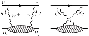
Figure 1: The $\gamma W$-box diagrams for the semileptonic decay process $H_{i}\to H_{f}e\bar{\nu}_{e}$.

The spin-independent part of $T^{VA}_{\mu\nu}$ has only one term, $T^{VA}_{\mu\nu}=i\epsilon_{\mu\nu\alpha\beta}q^{\alpha}p^{\beta}T_{3}+\dots$, where $T_{3}$ is a scalar function. For the neutron beta decay, the spin-dependent contributions, denoted by the ellipses here, are absorbed into the definition of the nucleon axial charge $g_{A}$, which can be measured directly from experiments. According to current algebra Sirlin (1978), it is this spin-independent term that gives rise to the hadron structure-dependent contribution and dominates the uncertainty in the theoretical prediction. Using $T_{3}$ as input, the axial $\gamma W$-box correction to the tree-level amplitude is given as Seng et al. (2018)

$$\Box_{\gamma W}^{VA}\big{|}_{H}=\frac{1}{F_{+}^{H}}\frac{\alpha_{e}}{\pi}\int_{0}^{\infty}dQ^{2}\,\frac{m_{W}^{2}}{m_{W}^{2}+Q^{2}}$$

$$\hskip 42.67912pt\times\int_{-\sqrt{Q^{2}}}^{\sqrt{Q^{2}}}\frac{dQ_{0}}{\pi}\frac{(Q^{2}-Q_{0}^{2})^{\frac{3}{2}}}{(Q^{2})^{2}}T_{3}(Q_{0},Q^{2}).$$ (2)

Here $Q^{2}=-q^{2}>0$ is the spacelike four-momentum square. The normalization factor $F_{+}^{H}$ arises from the local matrix element $\langle H_{f}(p^{\prime})|J_{\mu}^{W,V}|H_{i}(p)\rangle=(p+p^{\prime})_{\mu}F_{+}^{H}$, with $F_{+}^{H}=1$ for the neutron and $\sqrt{2}$ for the pion decay.

Methodology – In the framework of lattice QCD, the hadronic tensor $T^{VA}_{\mu\nu}$ in Euclidean spacetime is given by

$$T^{VA}_{\mu\nu}=\frac{1}{2}\int dt\,e^{-iQ_{0}t}\int d^{3}x\,e^{-i\vec{Q}\cdot\vec{x}}\,\mathcal{H}^{VA}_{\mu\nu}(t,\vec{x})$$ (3)

with $\mathcal{H}^{VA}_{\mu\nu}(t,\vec{x})$ defined as

$$\mathcal{H}^{VA}_{\mu\nu}(t,\vec{x})\equiv\langle H_{f}(P)|T\left[J^{em}_{\mu}(t,\vec{x})J^{W,A}_{\nu}(0)\right]|H_{i}(P)\rangle.$$ (4)

Here the Euclidean momenta $P$ and $Q$ are chosen as

$$P=(im_{H},\vec{0}),\quad Q=(Q_{0},\vec{Q})$$ (5)

with $m_{H}$ the hadron mass.

By multiplying $\epsilon_{\mu\nu\alpha\beta}Q_{\alpha}P_{\beta}$ to $T^{VA}_{\mu\nu}$, we can extract the function $T_{3}(Q_{0},Q^{2})$ through

$$T_{3}(Q_{0},Q^{2})=-\frac{\mathcal{I}}{2m_{H}^{2}|\vec{Q}|^{2}},\quad\mathcal{I}=\epsilon_{\mu\nu\alpha\beta}Q_{\alpha}P_{\beta}T^{VA}_{\mu\nu}.$$ (6)

Here $\mathcal{I}$ can be written in terms of $\mathcal{H}^{VA}_{\mu\nu}$ as

$$\mathcal{I} = \frac{i}{2}\epsilon_{\mu\nu\alpha 0}Q_{\alpha}m_{H}\int dt\,e^{-iQ_{0}t}\int d^{3}\vec{x}\,e^{-i\vec{Q}\cdot\vec{x}}\mathcal{H}^{VA}_{\mu\nu}$$ (7)

$$= \frac{m_{H}}{2}\int dt\,e^{-iQ_{0}t}\int d^{3}\vec{x}\,e^{-i\vec{Q}\cdot\vec{x}}\epsilon_{\mu\nu\alpha 0}\frac{\partial\mathcal{H}^{VA}_{\mu\nu}}{\partial x_{\alpha}}.$$

We can average over the spatial directions for $\vec{Q}$ and have

$$\mathcal{I} = \frac{m_{H}}{2}\int dt\,e^{-iQ_{0}t}\int d^{3}\vec{x}\,j_{0}\left(|\vec{Q}||\vec{x}|\right)\epsilon_{\mu\nu\alpha 0}\frac{\partial\mathcal{H}^{VA}_{\mu\nu}}{\partial x_{\alpha}}$$

$$= \frac{m_{H}}{2}\int dt\,e^{-iQ_{0}t}\int d^{3}\vec{x}\,\frac{|\vec{Q}|}{|\vec{x}|}j_{1}\left(|\vec{Q}||\vec{x}|\right)\epsilon_{\mu\nu\alpha 0}x_{\alpha}\mathcal{H}^{VA}_{\mu\nu},$$

where $j_{n}(x)$ are the spherical Bessel functions. A key ingredient in this approach is that once the Lorentz scalar function $\epsilon_{\mu\nu\alpha 0}x_{\alpha}\mathcal{H}^{VA}_{\mu\nu}$ is prepared, e.g. from a lattice QCD calculation, one can determine $T_{3}(Q_{0},Q^{2})$ directly.

Putting Eqs. (First-principles calculation of electroweak box diagrams from lattice QCD) and (6) into Eq. (First-principles calculation of electroweak box diagrams from lattice QCD) and changing the variables as $|\vec{Q}|=\sqrt{Q^{2}}\cos\theta$ and $Q_{0}=\sqrt{Q^{2}}\sin\theta$, we obtain the master formula

$$\Box_{\gamma W}^{VA}\big{|}_{H}=\frac{3\alpha_{e}}{2\pi}\int\frac{dQ^{2}}{Q^{2}}\,\frac{m_{W}^{2}}{m_{W}^{2}+Q^{2}}M_{H}(Q^{2})$$ (9)

with

$$M_{H}(Q^{2})=-\frac{1}{6}\frac{1}{F_{+}^{H}}\frac{\sqrt{Q^{2}}}{m_{H}}\int d^{4}x\,\omega(t,\vec{x})\epsilon_{\mu\nu\alpha 0}x_{\alpha}\mathcal{H}^{VA}_{\mu\nu}(t,\vec{x}),$$

$$\omega(t,\vec{x})=\int_{-\frac{\pi}{2}}^{\frac{\pi}{2}}\frac{\cos^{3}\theta\,d\theta}{\pi}\frac{j_{1}\left(\sqrt{Q^{2}}|\vec{x}|\cos\theta\right)}{|\vec{x}|}\cos\left(\sqrt{Q^{2}}t\sin\theta\right).$$

For small $Q^{2}$, lattice QCD can determine the function $M_{H}(Q^{2})$ with lattice discretization errors under control.

For large $Q^{2}$, we utilize the operator product expansion

$$\frac{1}{2}\int d^{4}xe^{-iQx}T\left[J_{\mu}^{em}(x)J_{\nu}^{W,A}(0)\right]$$ (11)

$$= \frac{i}{2Q^{2}}\left\{C_{a}(Q^{2})\delta_{\mu\nu}Q_{\alpha}-C_{b}(Q^{2})\delta_{\mu\alpha}Q_{\nu}\right.$$

$$\hskip 56.9055pt\left.-C_{c}(Q^{2})\delta_{\nu\alpha}Q_{\mu}\right\}J^{W,A}_{\alpha}(0)$$

$$+\frac{1}{6Q^{2}}C_{d}(Q^{2})\epsilon_{\mu\nu\alpha\beta}Q_{\alpha}J^{W,V}_{\beta}(0)+\cdots.$$

There are only four possible local operators at leading twist. (For the pion decay, the hadronic matrix elements for the first three operators vanish.) Multiplying $\epsilon_{\mu\nu\alpha\beta}Q_{\alpha}P_{\beta}$ to the relation (11) we obtain

$$T_{3}(Q_{0},Q^{2})=\frac{C_{d}(Q^{2})}{3Q^{2}}F_{+}^{H}+\cdots,$$

$$M_{H}(Q^{2})=\frac{C_{d}(Q^{2})}{12}+\cdots,$$ (12)

where the ellipses remind us that the higher-twist contributions are not included yet. The Wilson coefficient $C_{d}(Q^{2})$ is calculated to four-loop accuracy Larin and Vermaseren (1991); Baikov et al. (2010)

$$C_{d}(Q^{2})=\sum_{n}c_{n}a_{s}^{n},\quad a_{s}=\frac{\alpha_{s}(Q^{2})}{\pi},$$ (13)

with coefficients $c_{n}$ given in Eq. (12) of Ref. Baikov et al. (2010). Here $\alpha_{s}$ is the strong coupling constant.

We introduce a momentum-squared scale $Q^{2}_{\mathrm{cut}}$ that separates the two regimes, and split the integral in Eq. (9) into two parts

$$\Box_{\gamma W}^{VA}\big{|}_{H} = \Box_{\gamma W}^{VA,\leq}\big{|}_{H}+\Box_{\gamma W}^{VA,>}\big{|}_{H}$$

$$= \left(\int_{0}^{Q^{2}_{\mathrm{cut}}}\frac{dQ^{2}}{Q^{2}}+\int_{Q^{2}_{\mathrm{cut}}}^{\infty}\frac{dQ^{2}}{Q^{2}}\right)\frac{m_{W}^{2}}{m_{W}^{2}+Q^{2}}M_{H}(Q^{2}).$$

With Eq. (First-principles calculation of electroweak box diagrams from lattice QCD) we use the lattice data to determine the integral for $Q^{2}\leq Q^{2}_{\mathrm{cut}}$, while with Eq. (First-principles calculation of electroweak box diagrams from lattice QCD) we use perturbation theory to determine the integral for $Q^{2}>Q^{2}_{\mathrm{cut}}$.

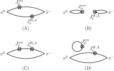
Figure 2: Four types of quark contractions for pion $\gamma W$-box diagrams.

Lattice setup – We use five lattice QCD gauge ensembles at the physical pion mass, generated by RBC and UKQCD Collaborations using $2+1$-flavor domain wall fermion Blum et al. (2016). The ensemble parameters are shown in Table 1. Here 48I and 64I use the Iwasaki gauge action in the simulation (denoted as Iwasaki in this work) while the other three ensembles use Iwasaki+DSDR action (denoted as DSDR). We calculate the correlation function $\langle\phi_{\pi^{0}}(t_{f})J_{\mu}^{em}(x)J_{\nu}^{W,A}(y)\phi_{\pi^{-}}^{\dagger}(t_{i})\rangle$ with $t_{f}=\operatorname{max}\{t_{x},t_{y}\}+\Delta t$ and $t_{i}=\operatorname{min}\{t_{x},t_{y}\}-\Delta t$. We use the wall-source pion interpolating operators $\phi_{\pi^{0}}$ and $\phi_{\pi^{-}}^{\dagger}$, which have a good overlap with the $\pi$ ground state, and find the ground-state saturation for $\Delta t\gtrsim 1$ fm. In practice the values of $\Delta t$ are chosen conservatively as shown in Table 1. For each ensemble we use the gauge configurations with sufficiently long separation, i.e. each separated by at least 10 trajectories. The number of configurations used is listed in Table 1.

Ensemble	$m_{\pi}$ [MeV]	$L$	$T$	$a^{-1}$ [GeV]	$N_{\text{conf}}$	$N_{r}$	$\Delta t/a$
24D	141.2(4)	$24$	$64$	$1.015$	46	1024	8
32D	141.4(3)	$32$	$64$	$1.015$	32	2048	8
32D-fine	143.0(3)	$32$	$64$	$1.378$	71	1024	10
48I	135.5(4)	$48$	$96$	$1.730$	28	1024	12
64I	135.3(2)	$64$	$128$	$2.359$	62	1024	18

Table 1: Ensembles used in this work. For each ensemble we list the pion mass $m_{\pi}$, the spatial and temporal extents, $L$ and $T$, the inverse of lattice spacing $a^{-1}$, the number of configurations used, $N_{\text{conf}}$, the number of point-source light-quark propagator generated for each configuration, $N_{r}$, and the time separation, $\Delta t$, used for the $\pi$ ground-state saturation.

There are four types of contractions for $\gamma W$-box diagrams as shown in Fig. 2. We produce wall-source quark propagators on all time slices. Using the techniques described in Ref. Tuo et al. (2019) type (A) and (B) diagrams can be calculated with high precision by performing the spacetime-translation average over $L^{3}\times T$ measurements. Under the $\gamma_{5}$ Hermitian conjugation of the Euclidean quark propagators, one can confirm that type (B) does not contribute to the axial $\gamma W$-box diagrams. Type (C) diagram is calculated by treating one current as the source and the other as the sink. We calculate point-source propagators at $N_{r}$ random spacetime locations. The values of $N_{r}$ are shown in Table 1. These point-source propagators can be placed at either electromagnetic current or weak current. We thus average the type (C) correlation functions over $2\,N_{r}$ measurements. This is similar with the treatment taken by Ref. Feng et al. (2019b). We neglect the disconnected contribution (D), which vanishes in the flavor $SU(3)$ limit.

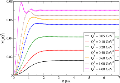
Figure 3: For ensemble 64I, lattice results of $M_{\pi}(Q^{2})$ as a function of the integral range $R$.

Numerical results – In practice, the integral in Eq. (First-principles calculation of electroweak box diagrams from lattice QCD) can be performed within a range of $\sqrt{t^{2}+\vec{x}^{2}}\leq R$. Taking the ensemble 64I as an example, $M_{\pi}(Q^{2})$ as a function of the integral range $R$ is shown in Fig. 3. We find that for all the momenta $Q^{2}\in[0,4]$ GeV², the integral is saturated at large $R$. We choose the truncation range $R_{0}\simeq 4$ fm, which is a conservative choice for all ensembles listed in Table 1. The contributions to the integral from $\sqrt{t^{2}+\vec{x}^{2}}>R_{0}$ is negligible, indicating that the finite-volume effects are well under control in our calculation. We can further verify this conclusion by a direct comparison using the 24D and 32D data.

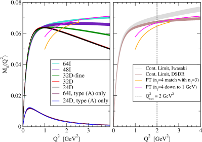
Figure 4: $M_{\pi}(Q^{2})$ as a function of $Q^{2}$. In the left panel, the lattice results for ensembles 64I, 48I, 32D-fine, 32D and 24D are represented by turquoise, indigo, dark green, red and black bands, respectively. Taking 64I and 24D as examples, the results for type (A) diagram are also plotted. In the right panel, Iwasaki and DSDR results at the continuum limit are shown by the gray and brown bands. The orange curve shows the results from perturbation theory by decoupling the charm quark at 1.6 GeV while the magenta one is compiled using the 4-flavor perturbation theory continuously down to 1 GeV.

The lattice results of $M_{\pi}(Q^{2})$ as a function of $Q^{2}$ are shown in Fig. 4 together with the perturbative results. Ensemble 24D and 32D have the same pion mass and lattice spacing but different volumes. The good agreement between these two ensembles indicates that the finite-volume effects are smaller than the statistical errors. At $Q^{2}\gtrsim 1$ GeV², the lattice discretization effects dominate the uncertainties. In the left panel of Fig. 4 an obvious discrepancy is observed at large $Q^{2}$ for the lattice results with different lattice spacings.

For the perturbation theory, the Wilson coefficient $C_{d}(Q^{2})$ is determined using the RunDec package Chetyrkin et al. (2000), where $\alpha_{s}$ is calculated to four-loop accuracy. At low $Q^{2}$ the results still contain large systematic uncertainties due to the lack of higher-loop and higher-twist contributions. In Fig. 4 we show two curves from perturbation theory. One is compiled using 4-flavor theory down to 1 GeV, while the other decouples the charm quark at 1.6 GeV and uses 3-flavor theory for $(\mbox{1 GeV})^{2}\leq Q^{2}\leq(\mbox{1.6 GeV})^{2}$. The discrepancy between the two curves suggests an O(14%) systematic effect in the perturbative determination of $M_{H}(Q^{2})$ at $Q^{2}\approx 1$ GeV².

Estimate of systematic effects – For $\Box_{\gamma W}^{VA,\leq}$ the largest uncertainties arise from the lattice discretization effects. Since Iwasaki and DSDR ensembles have different lattice discretizations, we treat them separately. After the linear extrapolation in $a^{2}$, the Iwasaki and DSDR results at continuum limit are shown in the right panel of Fig. 4. Using $Q_{\mathrm{cut}}^{2}=2$ GeV² we obtain

$$\Box_{\gamma W}^{VA,\leq}\big{|}_{\pi}=\begin{cases}0.671(11)\times 10^{-3}&\mbox{for Iwasaki}\\ 0.647(7)\times 10^{-3}&\mbox{for DSDR}\end{cases}.$$ (15)

We take the Iwasaki result as the central value and estimate the residual $O(a^{4})$ lattice artifacts using the discrepancy between Iwasaki and DSDR.

For $\Box_{\gamma W}^{VA,>}$ the largest uncertainties arise from the higher-loop and higher-twist truncation effects. We estimate the former by comparing the 4-loop and 3-loop results from perturbation theory. For the latter, unfortunately the complete information is not available. Considering the fact that type (A) diagram, which has two currents located at different quarks lines, only contains the higher-twist contributions, we use it to estimate the size of higher twist. At $Q_{\mathrm{cut}}^{2}=2$ GeV² we have

$$\Box_{\gamma W}^{VA,>}\big{|}_{\pi}=2.159(6)_{\mathrm{HL}}(7)_{\mathrm{HT}}\times 10^{-3},$$ (16)

where the central value is compiled using the 4-flavor theory (see the magenta curve in the right panel of Fig. 4). The first error indicates the higher-loop effects. The second one stands for the higher-twist effects, which are compiled from the integral of $Q^{2}>Q_{\mathrm{cut}}^{2}$ using the type (A) data as input.

Summary of results – After combining the results of $\Box_{\gamma W}^{VA,\leq}$ from lattice QCD and $\Box_{\gamma W}^{VA,>}$ from perturbation theory, we obtain the total contribution of $\Box_{\gamma W}^{VA}$

$$\Box_{\gamma W}^{VA}\big{|}_{\pi} = 2.830(11)_{\mathrm{stat}}(9)_{\mathrm{PT}}(24)_{\mathrm{a}}(3)_{\mathrm{FV}}\times 10^{-3}$$ (17)

$$= 2.830(11)_{\mathrm{stat}}(26)_{\mathrm{sys}}\times 10^{-3},$$

where the first uncertainty is statistical, and the remaining errors account for perturbative truncation and higher-twist effects, lattice discretization effects, and lattice finite-volume effects by comparing the 24D and 32D results. We add these systematic errors in quadrature to obtain the final systematic error. For comparison, we also calculate $\Box_{\gamma W}^{VA}\big{|}_{\pi}=2.816(9)_{\mathrm{stat}}(24)_{\mathrm{PT}}(18)_{\mathrm{a}}(3)_{\mathrm{FV}}\times 10^{-3}$ at $Q_{\mathrm{cut}}^{2}=1$ GeV² and $\Box_{\gamma W}^{VA}\big{|}_{\pi}=2.835(12)_{\mathrm{stat}}(5)_{\mathrm{PT}}(30)_{\mathrm{a}}(3)_{\mathrm{FV}}\times 10^{-3}$ at $Q_{\mathrm{cut}}^{2}=3$ GeV². Both results are consistent with Eq. (17).

For the pion semileptonic decay, the PIBETA experiment Pocanic et al. (2004) has improved the measurement of the branching ratio to 0.6%. The Standard Model prediction of the decay rate is given by Sirlin (1978); Pocanic et al. (2004)

$$\Gamma_{\pi\ell 3}=\frac{G_{F}^{2}|V_{ud}|^{2}m_{\pi}^{5}|f_{+}^{\pi}(0)|^{2}}{64\pi^{3}}\left(1+\delta\right)I_{\pi}$$ (18)

with $G_{F}=1.1663787(6)\times 10^{-5}\>\mathrm{GeV}^{-2}$ the Fermi’s constant measured from the muon decay, $m_{\pi}$ the charged pion mass, $f_{+}^{\pi}(0)=1$ the tree-level semileptonic form factor and $I_{\pi}=7.376(1)\times 10^{-8}$ a known kinematic factor. Numerically, $\Gamma_{\pi l3}=0.3988(23)\>\mathrm{s}^{-1}$ after taking into account the updated value of $\pi^{+}\rightarrow e^{+}\nu(\gamma)$ branching ratio as an overall normalization Czarnecki et al. (2019). The effects of radiative corrections are contained in $\delta$. The existing analysis from chiral perturbation theory (ChPT) yields $\delta=0.0334(10)_{\mathrm{LEC}}(3)_{\mathrm{HO}}$ Jaus (2001); Cirigliano et al. (2003); Passera et al. (2011); Czarnecki et al. (2019) with an overall theoretical uncertainty of $\Gamma_{\pi\ell 3}$ at a level of $0.1\%$. Here the first error is from the low energy constants and the second is the uncertainty in determining the higher-order QED effects Erler (2004). Thus the experimental measurement dominates the uncertainties and results in the determination of $|V_{ud}|=0.9739(28)_{\mathrm{exp}}(5)_{\mathrm{th}}$ with a 0.3% uncertainty.

We now show how our calculation reduces the uncertainty in $\delta$. We adopt Sirlin’s parameterization Sirlin (1978) with slight modifications:

$$\delta=\frac{\alpha_{e}}{2\pi}\left[\bar{g}+3\ln\frac{m_{Z}}{m_{p}}+\ln\frac{m_{Z}}{m_{W}}+\tilde{a}_{g}\right]+\delta_{\mathrm{HO}}^{\mathrm{QED}}+2\Box_{\gamma W}^{VA}.$$ (19)

By separating the axial $\gamma W$-box part into $\Box_{\gamma W}^{VA}$, the remaining contributions are model independent and are given as follows.

• Sirlin’s function $\bar{g}$ arises from a structure-indepenent, UV-finite one-loop integral. It accounts for the infrared contributions involving the vector $\gamma W$-box and the bremsstrahlung corrections. It contains a $3\ln m_{p}$ term that cancels the $m_{p}$-dependence in $3\ln\frac{m_{Z}}{m_{p}}$. Here $m_{p}$ is the proton mass that appears just as a matter of convention. Numerically, one has $\frac{\alpha_{e}}{2\pi}\bar{g}=1.051\times 10^{-2}$ Sirlin (1978); Wilkinson and Macefield (1970).

• $\tilde{a}_{g}$ represents the $O(\alpha_{s})$ QCD correction to all one-loop diagrams except for the axial $\gamma W$ box. The integral in $\tilde{a}_{g}$ is dominated by the high-energy scale $Q^{2}\simeq m_{W}^{2}$, where $\alpha_{s}$ is small. As a consequence $\frac{\alpha_{e}}{2\pi}\tilde{a}_{g}\approx-9.6\times 10^{-5}$ is a small contribution Sirlin (1978); Seng et al. (2020a).

• $\delta_{\mathrm{HO}}^{\mathrm{QED}}=0.0010(3)$ summarizes the leading-log higher-order QED effects which can be accounted for through the running of $\alpha_{e}$. The uncertainty assignment follows Ref. Erler (2004).

Although the detailed uncertainties for $\bar{g}$ and $\tilde{a}_{g}$ are not given, by power counting the intrinsic precision for the terms in the square brackets (multiplied by $\frac{\alpha_{e}}{2\pi}$) is of the order $G_{F}m_{p}^{2}\sim 10^{-5}$.

Combining the $\Box_{\gamma W}^{VA}$ in Eq. (17), we now obtain

$$\delta=0.0332(1)_{\gamma W}(3)_{\mathrm{HO}},$$ (20)

which corresponds to an almost complete removal of the dominant LEC uncertainties in the ChPT expression, and a reduction of the total uncertainty by a factor of 3. Therefore, any theoretical improvement in the future will unavoidably require a complete electroweak two-loop analysis. Consequently, the $|V_{ud}|$ determined from the pion semileptonic decay now reads: $|V_{ud}|=0.9740(28)_{\mathrm{exp}}(1)_{\mathrm{th}}$.

Conclusion – In this work we perform the first realistic lattice QCD calculation of the $\gamma W$-box correction to the pion semileptonic decay, $\Box_{\gamma W}^{VA}\big{|}_{\pi}$. The final result combines the lattice data at low momentum and perturbative calculation at high momentum. We use multiple lattice spacings and volumes at the physical pion mass to control the continuum and infinite-volume limits and obtain $\Box_{\gamma W}^{VA}\big{|}_{\pi}$ with a total error of $\sim 1$%. As a result, the uncertainty of the theoretical prediction for the pion semileptonic decay rates is reduced by a factor of $3$. This result does not impact the first-row CKM unitarity due to the large experimental error, but a follow-up work Seng et al. (2020b) shows that the 4-$\sigma$ tension persists.

The combined experimental measurement of 14 nuclear superallowed beta decays Hardy and Towner (2015) is 10 times more accurate than the current pion semileptonic decay experiment. On the other hand, the free neutron decay Tanabashi et al. (2018); Markisch et al. (2019) leads to a 4.5 times better precision. In these two cases, the nonperturbative, structure-dependent $\gamma W$-box contribution plays a decisive role. The technique presented in this work can be straightforwardly generalized to a lattice calculation of the nucleon $\gamma W$-box corrections, which are universal for both free and bound neutron decay. The latter is the key to a precise determination of $|V_{ud}|$ and a stringent test of CKM unitarity.