PyCARL: A PyNN Interface for Hardware-Software Co-Simulation of Spiking Neural Network

Abstract

We present PyCARL, a PyNN-based common Python programming interface for hardware-software co-simulation of spiking neural network (SNN). Through PyCARL, we make the following two key contributions. First, we provide an interface of PyNN to CARLsim, a computationally-efficient, GPU-accelerated and biophysically-detailed SNN simulator. PyCARL facilitates joint development of machine learning models and code sharing between CARLsim and PyNN users, promoting an integrated and larger neuromorphic community. Second, we integrate cycle-accurate models of state-of-the-art neuromorphic hardware such as TrueNorth, Loihi, and DynapSE in PyCARL, to accurately model hardware latencies, which delay spikes between communicating neurons, degrading performance of machine learning models. PyCARL allows users to analyze and optimize the performance difference between software-based simulation and hardware-oriented simulation. We show that system designers can also use PyCARL to perform design-space exploration early in the product development stage, facilitating faster time-to-market of neuromorphic products.

I Introduction

Advances in computational neuroscience have produced a variety of software for simulating spiking neural network (SNN) [1] — NEURON [2], NEST [3], PCSIM [4], Brian [5], MegaSim [6], and CARLsim [7]. These simulators model neural functions at various levels of detail and therefore have different requirements for computational resources.

In this paper, we focus on CARLsim [7], which facilitates parallel simulation of large SNNs using CPUs and multi-GPUs, simulates multiple compartment models, 9-parameter Izhikevich and leaky integrate-and-fire (LIF) spiking neuron models, and integrates the fourth order Runge Kutta (RK4) method for improved numerical precision. CARLsim’s support for built-in biologically realistic neuron, synapse, current and emerging learning models and continuous integration and testing, make it an easy to use and powerful simulator of biologically-plausible SNN models. Benchmarking results demonstrate simulation of 8.6 million neurons and 0.48 billion synapses using 4 GPUs and up to 60x speedup with multi-GPU implementations over a single-threaded CPU implementation.

To facilitate faster application development and portability across research institutes, a common Python programming interface called PyNN is proposed [8]. PyNN provides a high-level abstraction of SNN models, promotes code sharing and reuse, and provides a foundation for simulator-agnostic analysis, visualization and data-management tools. Many SNN simulators now support interfacing with PyNN — PyNEST [9] for the NEST simulator, PyPCSIM [4] for the PCSIM simulator, and Brian 2 [10] for the Brian simulator. Through PyNN, applications developed using one simulator can be analyzed/simulated using another simulator with minimal effort.

Currently, no interface exists between CARLsim, which is implemented in C++ and the Python-based PyNN. Therefore, applications developed in PyNN cannot be analyzed using CARLsim and conversely, CARLsim-based applications cannot be analyzed/simulated using other SNN simulators without requiring significant effort. This creates a large gap between these two research communities.

Our objective is to bridge this gap and create an integrated neuromorphic research community, facilitating joint developments of machine learning models and efficient code sharing. Figure 1 illustrates the standardized application programming interface (API) architecture in PyNN. Brian 2 and PCSIM, which are native Python implementations, employ a direct communication via the pynn.brian and pynn.pcsim API calls, respectively. NEST, on the other hand, is not a native Python simulator. So, the pynn.nest API call first results in a code generation to the native SLI code, a stack-based language derived from PostScript. The generated code is then used by the Python interpreter PyNEST to simulate an SNN application utilizing the backend NEST simulator kernel. Figure 1 also shows our proposed interface for CARLsim, which is exposed via the new pynn.carlsim API in PyNN. We describe this interface in details in Section III.

On the hardware front, neuromorphic computing [11] has shown significant promise to fuel the growth of machine learning, thanks to low-power design of neuron circuits, distributed implementation of computing and storage, and integration of non-volatile synaptic memory. In recent years, several spiking neuromorphic architectures are designed: SpiNNaker [12], DYNAP-SE [13], TrueNorth [14] and Loihi [15]. Unfortunately, due to non-zero latency of hardware components, spikes between communicating neurons may experience non-deterministic delays, impacting SNN performance.

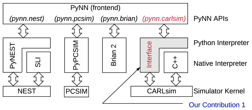
Figure 1: PyNN standardized API architecture and our proposed pynn-to-carlsim interface.

Currently, no PyNN-based simulators incorporate neuromorphic hardware laterncies. Therefore, SNN performance estimated using PyNN can be different from the performance obtained on hardware. Our objective is to estimate this performance difference, allowing users to optimize their machine learning model to meet a desired performance on a target neuromorphic hardware. Figure 2 shows our proposed carlsim-to-hardware interface to model state-of-the-art neuromorphic hardware at a cycle-accurate level, using the output generated from the proposed pynn-to-carlsim interface (see Figure 1). We describe this interface in Sec. IV.

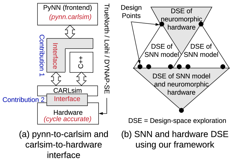
Figure 2: (a) Our proposed interface to estimate SNN performance on neuromorphic hardware and (b) design space exploration (DSE) based on this contribution.

The two new interfaces developed in this work can be integrated inside a design-space exploration (DSE) framework (illustrated in Figure 2(b)) to explore different SNN topologies and neuromorphic hardware configurations, optimizing both SNN performance such as accuracy and hardware performance such as latency, energy, and throughput.

Summary: To summarize, our comprehensive co-simulation framework, which we call PyCARL, allows CARLsim-based detailed software simulations, hardware-oriented simulations, and neuromorphic design-space explorations, all from a common PyNN frontend, allowing extensive portability across different research institutes. By using cycle-accurate models of state-of-the-art neuromorphic hardware, PyCARL allows users to perform hardware exploration and performance estimation early during application development, accelerating the neuromorphic product development cycle.

II Our Integrated Framework PyCARL

Figure 3 shows a high-level overview of our integrated framework PyCARL, based on PyNN. An SNN model written in PyNN is simulated using the CARLsim backend kernel with the proposed pynn-to-carlsim interface (contribution 1). This generates the first output snn.sw.out, which consists of synaptic strength of each connection in the network and precise timing of spikes on these connections. This output is then used in the proposed carlsim-to-hardware interface, allowing simulating the SNN on a cycle-accurate model of a state-of-the-art neuromorphic hardware such as TrueNorth [14], Loihi [15], and DYNAP-SE [13]. Our cycle-accurate model generates the second output snn.hw.out, which consists of 1) hardware-specific metrics such as latency, throughput, and energy, and 2) SNN-specific metrics such as inter-spike interval distortion and disorder spike count (which we formulate and elaborate in Section IV). SNN-specific metrics estimate the performance drop due to non-zero hardware latencies.

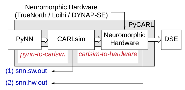
Figure 3: Our integrated framework PyCARL.

We now describe the components of PyCARL and show how to use PyCARL to perform design space explorations.

III Pynn-to-carlsim Interface in PyCARL

Apart from bridging the gap between the PyNN and the CARLsim research communities, the proposed pynn-to-carlsim interface is also significant in the following three ways. First, Python being an interactive language allows users to interact with the CARLsim kernel through command line, reducing the application development time. Second, the proposed interface allows code portability across different operating systems (OSes) such as Linux, Solaris, Windows, and Macintosh. Third, Python being open source, allows distributing the proposed interface with mainstream OS releases, exposing neuromorphic computing to the systems community.

An interface between Python (PyNN) and C++ (CARLsim) can be created using the following two approaches. First, through statically linking the C++ library with a Python interpreter. This involves copying all library modules used in CARLsim into a final executable image by an external program called linker or link editors. Statically linked files are significantly larger in size because external programs are built into the executable files, which must be loaded into the memory every time they are invoked. This increases program execution time. Static linking also requires all files to be recompiled every time one or more of the shared modules change. A second approach is the dynamic linking, which involves placing the names of the external libraries (shared libraries) in the final executable file while the actual linking taking place at run time. Dynamic linking is performed by the OS through API calls. Dynamic linking places only one copy of the shared library in memory. This significantly reduces the size of executable programs, thereby saving memory and disk space. Individual shared modules can be updated and recompiled, without compiling the entire source code again. Finally, load time of shared libraries is reduced if the shared library code is already present in memory. Due to lower execution time, reduced memory usage, and flexibility, we adopt dynamic linking of CARLsim with PyNN.

We now describe the two steps involved in creating the proposed pynn-to-carlsim interface.

III-A Step 1: Generating the Interface Binary carlsim.so

Unlike PyNEST, which generates the interface binary manually, we propose to use the Simplified Wrapper Interface Generator (SWIG), downloadable at http://www.swig.org. SWIG simplifies the process of interfacing high level languages such as Python with low-level languages such as C/C++, preserving the robustness and expressiveness of these low-level languages from the high-level abstraction.

The SWIG compiler creates a wrapper binary code by using headers, directives, macros, and declarations from the underlying C++ code of CARLsim. Figures 4-8 show the different components of the input file carlsim.i needed to generate the compiled interface binary file carlsim.so. The first component are the interface files that are included using the %include directive (Figure 4). The second component consists of declaration of the data structures (e.g., vectors) of CARLsim using the %template directive (Figure 5). The third component is the main module definition that can be loaded in Python using the import command (Figure 6).

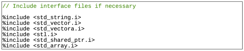
Figure 4: Define interface files using the %include directive.

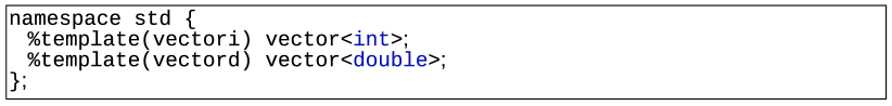
Figure 5: Declare CARLsim data structures using the %template directive.

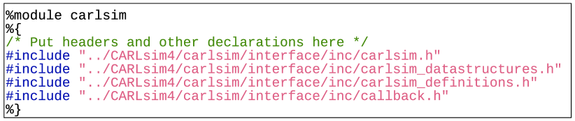
Figure 6: Main module definition for import in Python.

The fourth component consists of enumerated data types defined by the directive enum (Figure 7). In this example we show two definitions – 1) the STDP curve and 2) the computing platform. The last component is the CARLsim class object along with its member functions (Figure 8).

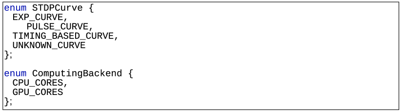
Figure 7: Enumerated data types using the enum directive.

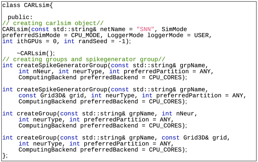
Figure 8: CARLsim class object.

The major advantage of using SWIG is that it uses a layered approach to generate a wrapper over C++ classes. At the lowest level, a collection of procedural ANSI-C style wrappers are generated by SWIG. These wrappers take care of the basic type conversions, type checking, error handling and other low-level details of C++ bindings. To generate the interface binary file carlsim.so, the input file carsim.i is compiled using the swig compiler as shown in Figure 9.

Figure 9: Compilation of carlsim.i using the SWIG compiler to generate carsim.so interface binary.

III-B Step 2: Designing PyNN API to Link carlsim.so

We now describe the proposed pynn.carlsim API to link the interface binary carlsim.so in PyNN.

The carlsim.so interface binary is placed within the sub-package directory of PyNN. This exposes CARLsim internal methods as a Python library using the import command as from carlsim import *. The PyNN front-end API architecture supports implementing both basic functionalities (common for all backend simulators) and specialized simulator-specific functionalities.

III-B1 Implementing common functionalities

PyNN defines many common functionalities to create a basic SNN model. Examples include cell types, connectors, synapses, and electrodes. Figure 10 shows the UML class diagram to create the Izhikevich cell type [16] using the pynn.carlsim API. The inheritance relationship shows that the PyNN standardmodels class includes the definition of all the methods under the StandardModelType class. The Izhikevich model and all similar standard cell types are a specialization of this StandardModelType class, which subsequently inherits from the PyNN BaseModelType class. Defining other standard components of an SNN model follow similar inheritance pattern using the common internal API functions provided by PyNN.

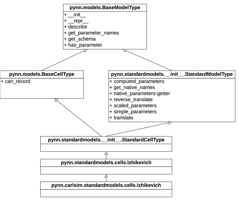
Figure 10: UML class diagram of Izhikevich cell type showing the relationship with the pynn.carlsim API.

III-B2 Implementing specialized CARLsim functions

Using the standard PyNN classes, it is also possible to define and expose non-standard CARLsim functionalities.

Figure 11 details the state class of CARLsim. The composition adornment relationship between the state class of the simulator module and the CARLsim class in the pynn.carlsim API. The composition adornment means that apart from the composition relationship between the contained class (CARLsim) and the container class (State), the object of the contained class also goes out of scope when the containing class goes out of scope. Thus, the State class exercises complete control over the members of the CARLsim class objects. The class member variable network of the simulator.State class contains an instance of the CARLsim object. From Figure 11 it can be seen that the CARLsim class consists of methods which can be used for the initial configuration of an SNN model and also methods for running, stopping and saving the simulation. These functions are appropriately exposed to the PyNN by including them in the pynn.carlsim API methods, which are created as members of the class simulator.State.

Figure 12 shows the implementations of the run() and setupNetwork() methods in the simulator.State class. It can be seen that these methods call the corresponding functions in the CARLsim class of the pynn.carlsim API. This technique can be used to expose other non-standard CARLsim methods in the pynn.carlsim API.

III-C Using pynn-to-carlsim Interface

To verify the integrity of our implementation, Figure 13 shows the source code of a test application written in PyNN. The source code sets SNN parameters using PyNN. A simple spike generation group with 1 neuron and a second neuron group with 3 excitatory Izhikevich neurons are created. The user can run the code in a CPU or a GPU mode by specifying the respective parameters in the command line.

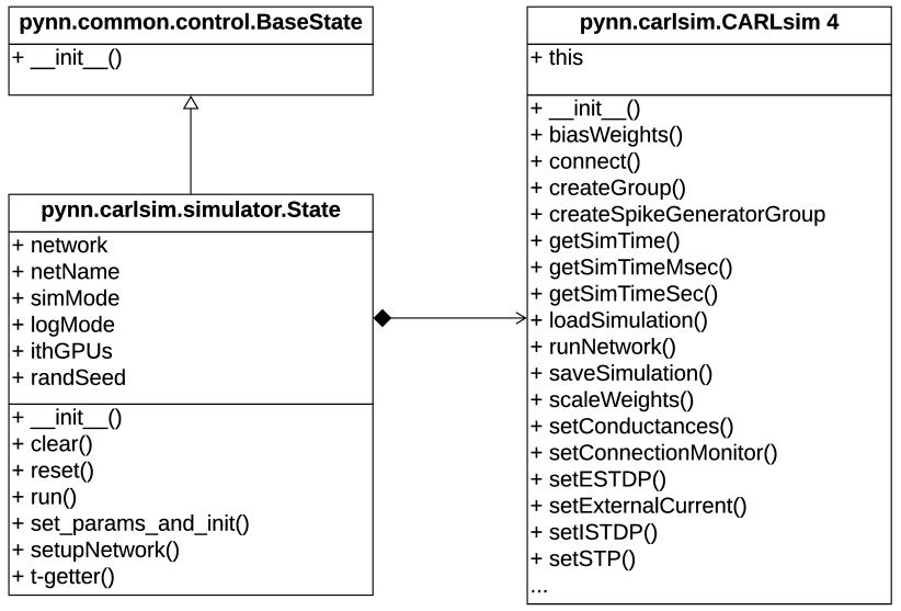
Figure 11: UML class diagram of simulator state of the pynn.carlsim API.

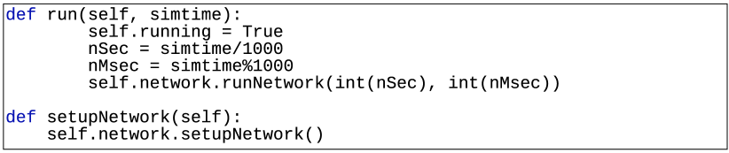
Figure 12: Snippet showing the exposed CARLsim functions in the pynn.carlsim API.

It can be seen from the figure that command line arguments have been specified to receive the simulator specific parameters from the user. This command line parameters can be replaced with custom defined methods in the pynn.carlsim API of PyNN or by using configuration files in xml or json format. The application code shows the creation of an SNN model by calling the get_simulator method. To use CARLsim back-end, an user must specify “carlsim” as the simulator to be used for this script while invoking the Python script, as can be seen in Figure 14. This results in the internal resolution of creating an instance of CARLsim internally by PyNN. The returned object (denoted as sim in the figure) is then used to access all the internal API methods offering the user control over the simulation.

Figure 15 shows the starting of the simulation by executing the command in Figure 14. As can be seen, the CPU_MODE is set by overriding the GPU_MODE as no argument was provided in the command and the default mode being CPU_MODE was set. The test is being run in the logger mode USER with a random seed of 42 as specified in the command line. From Figure 13, we see that the application is set in the current-based (CUBA) mode, which is also reported during simulation (Fig. 15). The timing parameters such as the AMPA decay time and the GABAb decay times are set in simulation as shown in Figure 13.

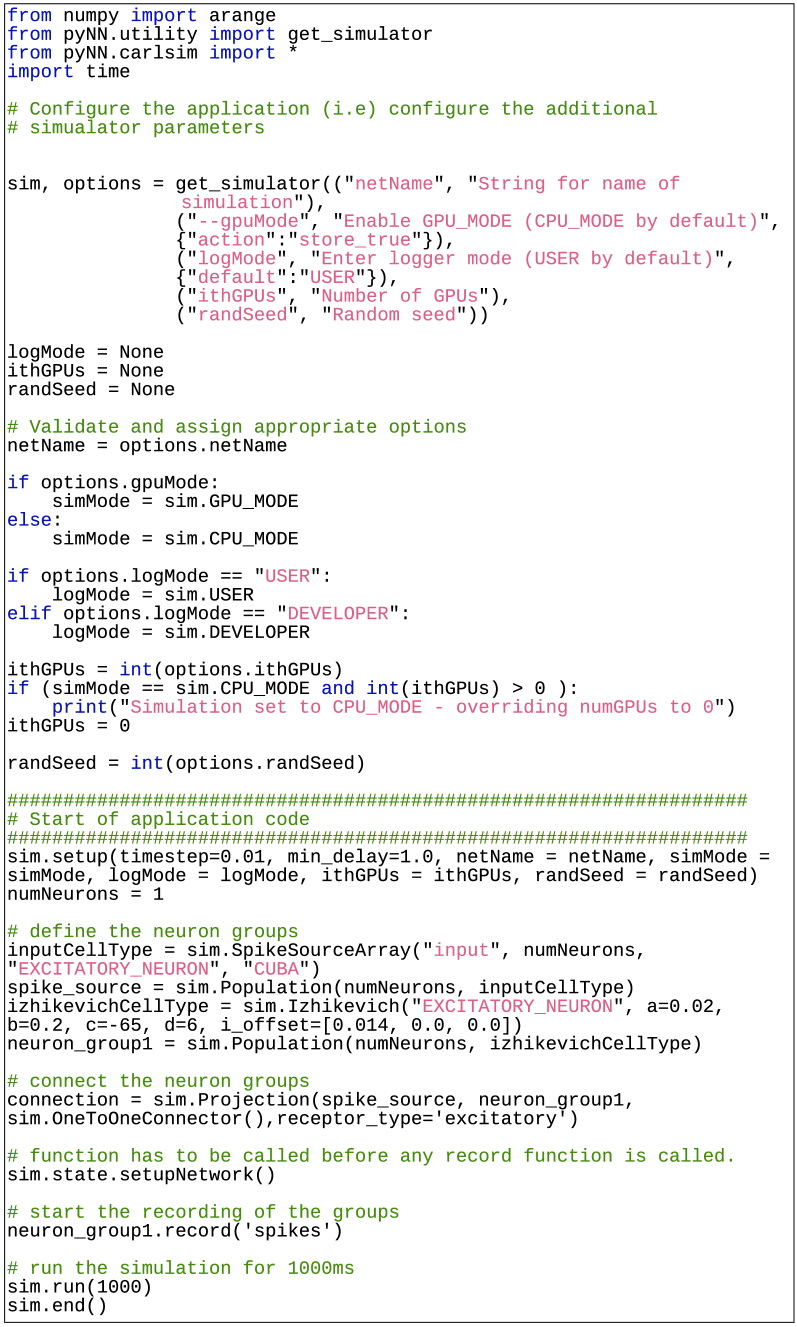
Figure 13: An example application code written in PyNN.

Figure 14: Executing the test application from command line.

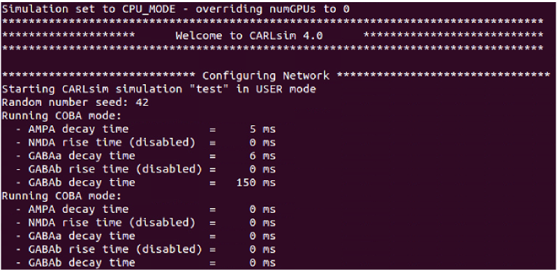
Figure 15: Simulation snippet.

III-D Generating Output snn.sw.out

At the end of simulation, the proposed pynn-to-carlsim interface generates the following information.

• Spike Data: the exact spike times of all neurons in the SNN model and stores them in a 2D spike vector. The first dimension of the vector is neuron id and the second dimension is spike times. Each element $spkVector[i]$ is thus a vector of all spike times for the $i^{\text{th}}$ neuron.

• Weight Data: the synaptic weights of all synapses in the SNN model and stores them in a 2D connection vector. The first dimension of the vector is the pre-synaptic neuron id and the second dimension is the post-synaptic neuron id. The element $synVector[i,j]$ is the synaptic weight of the connection $(i,j)$.

The spike and weight data can be used to analyze and adjust the SNN model. They form the output snn.sw.out of our integrated framework PyCARL.

IV Hardware-Oriented Simulation in PyCARL

To estimate the performance impact of executing SNNs on a neuromorphic hardware, the standard approach is to map the SNN to the hardware and measure the change in spike timings, which are then analyzed to estimate the performance deviation from software simulations. However, there are three limitations to this approach. First, neuromorphic hardware are currently in their research and development phase in a selected few research groups around the world. They are not yet commercially available to the bigger systems community. Second, neuromorphic hardware that are available for research have limitations on the number of synapses per neuron. For instance, DynapSE can only accommodate a maximum of 128 synapses per neuron. These hardware platforms therefore cannot be used to estimate performance impacts on large-scale SNN models. Third, existing hardware platforms have limited interconnect strategies for communicating spikes between neurons, and therefore they cannot be used to explore the design of scalable neuromorphic architectures that minimize latency, a key requirement for executing real-time machine learning applications. To address these limitations, we propose to design a cycle-accurate neuromorphic hardware simulator, which can allow the systems community to explore current and future neuromorphic hardware to simulate large SNN models and estimate the performance impact.

IV-A Designing Cycle-Accurate Hardware Simulator

Figure 16(a) shows the architecture of a neuromorphic hardware with multiple crossbars and a shared interconnect. Analogous to the mammalian brain, synapses of a SNN can be grouped into local and global synapses based on the distance information (spike) conveyed. Local synapses are short distance links, where pre- and post-synaptic neurons are located in the same vicinity. They map inside a crossbar. Global synapses are those where pre- and post-synaptic neurons are farther apart. To reduce power consumption of the neuromorphic hardware, the following strategies are adopted:

• the number of point-to-point local synapses is limited to a reasonable dimension (size of a crossbar); and

• instead of point-to-point global synapses (which are of long distance) as found in a mammalian brain, the hardware implementation usually consists of time-multiplexed interconnect shared between global synapses.

DYNAP-SE [13] for example, consists of four crossbars, each with 128 pre- and 128 post-synaptic neurons implementing a full 16K (128x128) local synapses per crossbar.

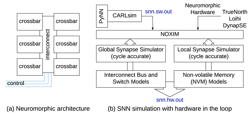
Figure 16: (a) Neuromorphic architecture and (b) SNN Simulations with hardware in the loop.

Since local synapses map within the crossbar, their latency is fixed and can be estimated offline. However, the global synapses are affected by variable latency introduced due to time multiplexing of the shared interconnect at run-time. Figure 16(b) shows the proposed framework for SNN simulation with hardware in the loop. The snn.sw.out generated from the pynn-to-carlsim interface is used as trace for the cycle-accurate simulator NOXIM [17]. NOXIM allows integration of circuit-level power-performance models of non-volatile memory (NVM), e.g., phase-change memory (PCM) for the crossbars and highly configurable global synapse model based on mesh architecture. The user configurable parameters include buffer size, network size, packet size, packet injection rate, routing algorithm, and selection strategy. In the power consumption simulation aspect, a user can modify the power values in external loaded YAML file to benefit from the flexibility. For the simulation results, NOXIM can calculate latency, throughput and power consumption automatically based on the statistics collected during runtime.

NOXIM has been developed using a modular structure that easily allows to add new interconnect models, which is an adoption of object-oriented programming methodology, and to experiment with them without changing the remaining parts of the simulator code. The cycle-accurate feature is provided via the SystemC programming language. This makes NOXIM the ideal framework to represent a neuromorphic hardware.

IV-A1 Existing NOXIM Metrics

As a traditional interconnect simulator, NOXIM provides performance metrics, which can be adopted to global synapse simulation directly.

• Latency: The difference between the sending and receiving time of spikes in number of cycles.

• Network throughput: The number of total routed spikes divided by total simulation time in number of cycles.

• Area and energy consumption: Area consumption is calculated based on the number of processing elements and routers; energy consumption is generated based on not only the number, but also their activation degree depending on the traffic. The area and energy consumption are high-level estimates for a given neuromorphic hardware. We adopt such high-level approach to keep the simulation speed sufficiently low, which is required to enable the early design space exploration.

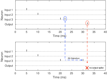
(a)

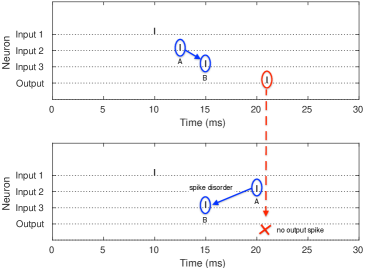
(b)

Figure 17: Impact of ISI distortion (a) and spike disorder (b) on the output spike for a simple SNN with three input neurons connected to a single output neuron.

IV-A2 New NOXIM Metrics

We introduce the following two new metrics to represent the performance impact of executing an SNN on the hardware.

• Disorder spike count: This is added for SNNs where information is encoded in terms of spike rate. We formulate spike disorder as follows. Let $F^{i}=\{F_{1}^{i},\cdots,F_{n_{i}}^{i}\}$ be the expected spike arrival rate at neuron $i$ and $\hat{F}^{i}=\{\hat{F}_{1}^{i},\cdots,\hat{F}_{n_{i}}^{i}\}$ be the actual spike rate considering hardware latencies. The spike disorder is computed as

  $$\footnotesize\text{spike disorder}=\sum_{j=1}^{n_{i}}[(F_{j}^{i}-\hat{F}_{j}^{i})^{2}]/n_{i}$$ (1)

• Inter-spike interval distortion: Performance of supervised machine learning is measured in terms of accuracy, which can be assessed from inter-spike intervals (ISIs) [18]. To define ISI, we let $\{t_{1},t_{2},\cdots,t_{K}\}$ be a neuron’s firing times in the time interval $[0,T]$. The average ISI of this spike train is given by [18]:

  $$\vspace{-5pt}\footnotesize\mathcal{I}=\sum_{i=2}^{K}(t_{i}-t_{i-1})/(K-1).$$ (2)

To illustrate how ISI distortion and spike disorder impact accuracy, we consider a small SNN example where three input neurons are connected to an output neuron. In Figure LABEL:fig:isi_imact, we illustrate the impact of ISI distortion on the output spike. In the top sub-figure, we observe that a spike is generated at the output neuron at 22ms due to spikes from the input neurons. In the bottom sub-figure, we observe that the second spike from input 3 is delayed, i.e., has ISI distortion. As a result of this distortion, there is no output spike. Missing spikes can impact application accuracy, as spikes encode information in SNNs. In Figure LABEL:fig:disorder_impact, we illustrate the impact of spike disorder on the output spike. In the top sub-figure, we observe that the spike A from input 2 is generated before the spike B from input 3, causing an output spike to be generated at 21ms. In the bottom sub-figure, we observe that the spike order of inputs 2 and 3 is reversed, i.e., the spike B is generated before the spike A. This spike disorder results in no spike being generated at the output neuron, which can also lead to a drop in accuracy.

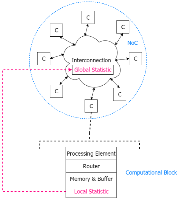
Figure 18: Statistics collection architecture in PyCARL.

IV-B Generating Output snn.hw.out

Figure 18 shows the statistics collection architecture in PyCARL. Overall, the output snn.hw.out consists of two performance components as highlighted in Table I.

snn.hw.out
hardware performance	specific to neuromorphic hardware
	latency, throughput, and energy
model performance	specific to SNN model
	disorder, inter-spike interval, and fanout

TABLE I: Performance metrics obtained in executing an SNN model on the neuromorphic hardware.

V Evaluation Methodology

V-A Simulation Environment

We conduct all experiments on a system with 8 CPUs, 32GB RAM, and NVIDIA Tesla GPU, running Ubuntu 16.04.

V-B Evaluated Applications

Table II reports the applications that we used to evaluate PyCARL. The application set consists of 7 functionality tests from the CARLsim and PyNN repositories. The CARLsim functionality tests are testKernel{1,2,3}. The PyNN functionality tests are Izhikevich, Connections, SmallNetwork, and Varying_Poisson. These functionalities verify the biological properties on neurons and synapses. Columns 2, 3 and 4 in the table reports the number of synapses, the SNN topology and the number of spikes simulated by these functionality tests.

Apart from the functionality tests, we evaluate PyCARL using large SNNs for 4 synthetic and 4 realistic applications. The synthetic applications are indicated with the letter ‘S’ followed by a number (e.g., S_1000), where the number represents the total number of neurons in the application. The 4 realistic applications are image smoothing (ImgSmooth) [7] on 64x64 images, edge detection (EdgeDet) [7] on 64x64 images using difference-of-Gaussian, multi-layer perceptron (MLP)-based handwritten digit recognition (MLP-MNIST) [19] on 28x28 images of handwritten digits and CNN-based heart-beat classification (HeartClass) using ECG signals [20, 21, 22].

Category	Applications	Synapses	Topology	Spikes
functionality tests	testKernel1	1	FeedForward (1, 1)	6
	testKernel2	101,135	Recurrent (Random)	96,885
	testKernel3	100,335	FeedForward (800, 200)	63,035
	Izhikevich	4	FeedForward (3, 1)	3
	Connections	7,200	Recurrent (Random)	1,439
	SmallNetwork	200	FeedForward (20, 20)	47
	Varying_Poisson	50	FeedForward (1, 50)	700
synthetic	S_1000	240,000	FeedForward (400, 400, 100)	5,948,200
	S_1500	300,000	FeedForward (500, 500, 500)	7,208,000
	S_2000	640,000	FeedForward (800, 400, 800)	45,807,200
	S_2500	1,440,000	FeedForward (900, 900, 700)	66,972,600
realistic	ImgSmooth [7]	136,314	FeedForward (4096, 1024)	17,600
	EdgeDet [7]	272,628	FeedForward (4096, 1024, 1024, 1024)	22,780
	MLP-MNIST [19]	79,400	FeedForward (784, 100, 10)	2,395,300
	HeartClass [20]	2,396,521	CNN1	1,036,485

• Input(82x82) - [Conv, Pool]*16 - [Conv, Pool]*16 - FC*256 - FC*6

TABLE II: Applications used for evaluating PyCARL.

VI Results and Discussion

VI-A Evaluating pynn-carlsim Interface of PyCARL

We evaluate the proposed pynn-to-carlsim interface in PyCARL using the following two performance metrics.

• Memory usage: This is the amount of main memory (DDDx) occupied by each application when simulated using PyCARL (Python). Main memory usage is reported in terms of the resident set size (in kB). Results are normalized to the native CARLsim simulation (in C++).

• Simulation time: This is the time consumed to simulate each application using PyCARL. Execution time is measured as CPU time (in ms). Results are normalized to the native CARLsim simulation.

VI-A1 Memory Usage

Figure 19 plots the memory usage of each application using PyCARL normalized to CARLsim. For easy reference, the absolute memory usage of CARLsim is also reported on the bar for each application. We make the following three main observations. First, the memory usage is application-dependent. The memory usage of testKernel1 with a single synapse is 6.9MB, compared to the memory usage of 151.4 MB for Synth_2500 with 1,440,000 synapses. Second, the memory usage of PyCARL is on average 3.8x higher than CARLsim. This is because 1) the pynn-carlsim interface loads all shared CARLsim libraries in the main memory during initialization, irrespective of whether or not they are utilized during simulation and 2) some of CARLsim’s dynamic data structures are re-created during SWIG compilation as SWIG cannot access these native data structures in the main memory. Our future work involves solving both these limitation to reduce the memory footprint of PyCARL. Third, smaller SNNs result in higher memory overhead. This is because for smaller SNNs, the memory allocation for CARLsim libraries becomes the primary contributor of the memory overhead in PyCARL. CARLsim, on the other hand, loads only the libraries that are needed for the SNN simulation.

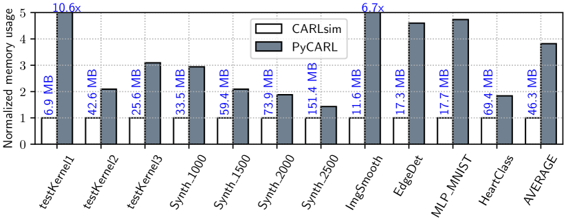
Figure 19: Memory usage of PyCARL normalized to CARLsim (out of scale results are reported on the bar).

VI-A2 Simulation Time

Figure 20 plots the simulation time of each our applications using PyCARL, normalized to CARLsim. For easy reference, the absolute simulation time of CARLsim is also reported on the bar for each application. We make the following two main observations. First, the simulation time using PyCARL is on average 4.7x higher than CARLsim. The high simulation time of PyCARL is contributed by two components – 1) initialization time, which includes the time to load all shared libraries and 2) the time for simulating the SNN. We observe that the simulation time of the SNN is comparable between PyCARL and CARLsim. The difference is in the initialization time of PyCARL, which is higher than CARLsim. Second, the overhead for smaller SNNs (i.e., ones with less number of spikes) are much higher because the initialization time dominates the overall simulation time for these SNNs, Therefore, PyCARL, which has higher initialization time, has higher simulation time than CARLsim.

To analyze the simulation time, Figure 21 plots the distribution of total simulation time into initialization time and the SNN simulation time. For testKernel1 with only 6 spikes (see Table II), the initialization time is over 99% of the total simulation time. Since the initialization time is considerably higher in PyCARL, the overall simulation time is 17.1x than CARLsim (see Figure 20). On the other hand, for a large SNN like Synth_2500, the initialization time is only 8% of the total simulation time. For this application PyCARL’s simulation time is only 4% higher than CARLsim.

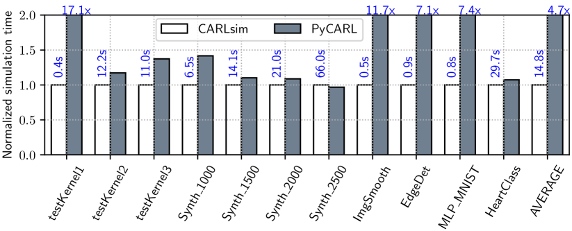
Figure 20: Simulation time of PyCARL normalized to CARLsim (out of scale results are reported on the bar).

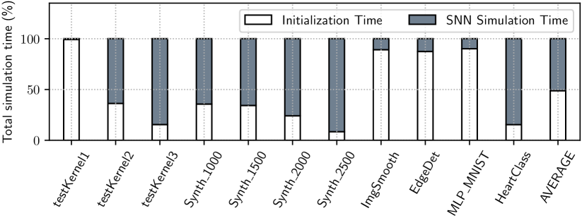
Figure 21: Total Simulation time distributed into initialization time and SNN simulation time.

We conclude that the total simulation time using PyCARL is only marginally higher than native CARLsim for larger SNNs, which are typical in most machine learning models. This is an important requirement to enable fast design space exploration early in the model development stage. Hardware-aware circuit-level simulators are much slower and have large memory footprint. Finally, other PyNN-based SNN simulators don’t have the hardware information so they can only provide functional checking of machine learning models.

VI-B Evaluating carlsim-hardware Interface of PyCARL

VI-B1 Hardware Configurations Supported in PyCARL

Table III reports the supported spike routing algorithms in PyCARL.

Algorithms	Description
XY	Packets first go horizontally and then vertically to reach destinations.
West First	West direction should be taken first if needed in the proposed route to destination.
North Last	North direction should be taken last if needed in the proposed route to destination.
Odd Even	Turning from the east at tiles located in even columns and turning to the west at tiles in odd column are prohibited.
DyAD	XY routing when there is no congestion, and Odd Even routing when there is congestion.

TABLE III: Routing algorithms supported in PyCARL.

To illustrate the statistics collection, we use a fully connected synthetic SNN with two feedforward layers of 18 neurons each. The SNN is mapped to a hardware with 36 crossbars arranged in a 6x6 mesh topology. Figure 22 shows a typical distribution of spike latency and ISI distortion (in clock cycles) collected when configuring the global synapse network with XY routing.

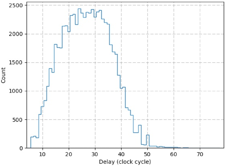
(a)

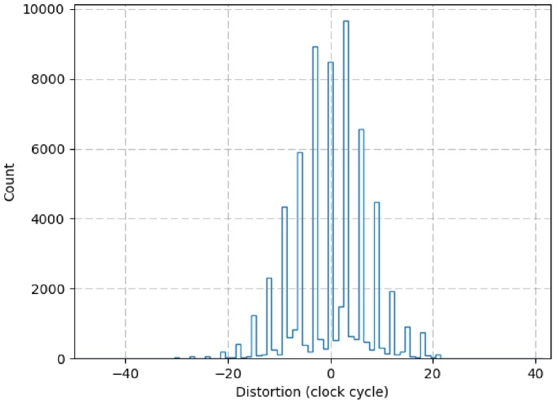
(b)

Figure 22: (a) Latency and (b) ISI distortion for XY routing.

Table IV reports the statistics collected for different routing algorithms for the global synapse network of the neuromorphic hardware. PyCARL facilitates system design exploration in the following two ways. First, system designers can explore these statistics and set a network configuration to achieve the desired optimization objective. In our prior work [23], we have developed segmented bus interconnect for neuromorphic hardware using PyCARL. Second, system designers can analyze these statistics for a given hardware to estimate performance of SNNs on hardware. In our prior work [24, 25, 26, 27], we have analyzed such performance deviation using PyCARL.

Algorithms	Avg. ISI	Disorder Count	Avg. Latency	Avg. Throughput
	(cycles)	(cycles)	(cycles)	(spikes/cycle)
XY	48	203	26.75	0.191
West First	44	198	26.76	0.191
North Last	43	185	26.77	0.191
Odd Even	44	176	26.77	0.191
DyAD	44	186	26.78	0.191

TABLE IV: Evaluating routing algorithms in PyCARL.

VI-B2 Performance Impact on Hardware

To illustrate how the performance of a machine learning application changes on hardware, Figure 23 shows the accuracy of MLP_MNIST obtained on five hardware configurations programmed in PyCARL. We also report the accuracy of MLP_MNIST obtained using software-only simulation with the proposed pynn-carlsim interface. The hardware configuration $n\times n~{}(m)$ is for a neuromorphic hardware with $n^{2}$ crossbars, arranged using a $n\times n$ mesh network. Each crossbar can accommodate $m$ input and $m$ output neurons, with a maximum of $m$ pre-synaptic connections per output neuron. We observe that compared to an accuracy of 89% obtained using the pynn-carlsim interface, the best case accuracy on a $6\times 6$ hardware ($36$ crossbars with $25$ input and $25$ output neurons per crossbar) is only 66.6% – a loss of $22.4\%$. This loss is due to hardware latencies, which delay some spikes more than others, and are not accounted when performing accuracy estimation through software-only simulations. The proposed carlsim-hardware interface in PyCARL facilitates estimating accuracy (performance in general) impact of machine learning applications on neuromorphic hardware.

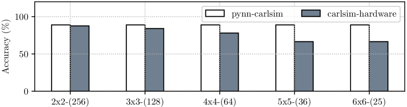
Figure 23: Accuracy of MLP_MNIST on five neuromorphic hardware configurations compared to the accuracy obtained via software-only simulation using pynn-carlsim interface.

VI-B3 SNN Performance on DYNAP-SE

Figure 24 evaluates the statistics collection feature of PyCARL on DYNAP-SE [13], a state-of-the-art neuromorphic hardware to estimate performance impact between software-only simulation (using pynn-carlsim interface) and hardware-oriented simulation (using carlsim-hardware interface) for each application.

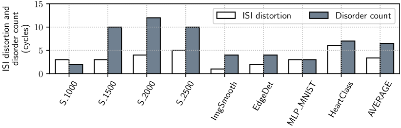
Figure 24: ISI distortion and disorder of hardware-oriented simulation, normalized to software-only simulation.

We observe that these applications have average ISI distortion of 3.375 cycles and disorder of 6.5 cycles when executed on the specific neuromorphic hardware. In the software-only simulation (using the pynn-carlsim interface), ISI distortion and disorder count are both zero. These design metrics directly influence performance, as illustrated in Figure 17.

VI-B4 Design Space Exploration using PyCARL

We now demonstrate how the statistics collection feature of PyCARL can be used to perform design space explorations optimizing hardware metrics such as latency and energy. We demonstrate PyCARL for DYNAP-SE using an instance of particle swarm optimization (PSO) [28] to distribute the synapses in order to minimize latency and energy. The mapping technique is adapted from our earlier published work [25]. Although optimizing SNN mapping to the hardware is not the main focus of this paper, the following results only illustrate the capability of PyCARL to perform such optimization.

Figure 25 plots the energy and latency of each application obtained using PyCARL, normalized to PyNN, which balances the synapses on different crossbars of the hardware. We observe that PyCARL achieves an average 50% lower energy and 24% lower latency than PyNN’s native load balancing strategy. These improvements clearly motivate the significance of PyCARL in advancing neuromorphic computing.

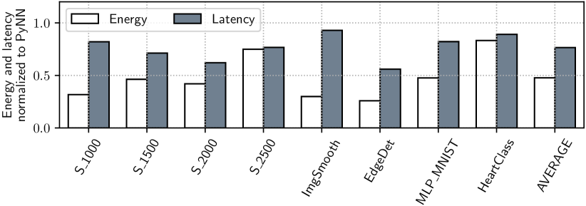
Figure 25: Energy and latency of PyCARL normalized to PyNN.

VII Conclusions

We present PyCARL, a Python programming interface that allows CARLsim-based spiking neural network simulations with neurobiological details at the neuron and synapse levels, hardware-oriented simulations, and design-space explorations for neuromorphic computing, all from a common PyNN frontend. PyCARL allows extensive portability across different research institutes. We evaluate PyCARL using functionality tests as well as synthetic and realistic SNN applications on a state-of-the-art neuromorphic hardware. By using cycle-accurate models of neuromorphic hardware, PyCARL allows users to perform neuromorphic hardware and machine learning model explorations and performance estimation early during application development, accelerating the neuromorphic product development cycle. We conclude that PyCARL is a comprehensive framework that has significant potential to advance the field of neuromorphic computing.

PyCARL is available for download at [29].

References

- [1] W. Maass, “Networks of spiking neurons: The third generation of neural network models,” Neural Networks, 1997.
- [2] M. L. Hines and N. T. Carnevale, “The NEURON simulation environment,” Neural Computation, 1997.
- [3] M.-O. Gewaltig and M. Diesmann, “Nest (neural simulation tool),” Scholarpedia, 2007.
- [4] D. Pecevski, T. Natschläger, and K. Schuch, “PCSIM: A parallel simulation environment for neural circuits fully integrated with Python,” Frontiers in Neuroinformatics, 2009.
- [5] D. F. Goodman and R. Brette, “Brian: A simulator for spiking neural networks in python,” Frontiers in Neuroinformatics, 2008.
- [6] B. Linares-Barranco, “The Modular Event-driven Growing Asynchronous Simulator (MegaSim),” https://bitbucket.org/bernabelinares/megasim, 2020.
- [7] T.-S. Chou, H. J. Kashyap, J. Xing, S. Listopad, E. L. Rounds, M. Beyeler, N. Dutt, and J. L. Krichmar, “CARLsim 4: An open source library for large scale, biologically detailed spiking neural network simulation using heterogeneous clusters,” in IJCNN, 2018.
- [8] A. P. Davison, D. Brüderle, J. M. Eppler, J. Kremkow, E. Muller, D. Pecevski, L. Perrinet, and P. Yger, “PyNN: a common interface for neuronal network simulators,” Frontiers in Neuroinformatics, 2009.
- [9] J. M. Eppler, M. Helias, E. Muller, M. Diesmann, and M.-O. Gewaltig, “PyNEST: A convenient interface to the NEST simulator,” Frontiers in Neuroinformatics, 2009.
- [10] S. Marcel and B. Romain, “Brian 2, an intuitive and efficient neural simulator,” eLife, 2019.
- [11] C. Mead, “Neuromorphic electronic systems,” Proc. of the IEEE, 1990.
- [12] S. B. Furber, F. Galluppi, S. Temple, and L. A. Plana, “The SpiNNaker project,” Proc. of the IEEE, 2014.
- [13] S. Moradi, N. Qiao, F. Stefanini, and G. Indiveri, “A scalable multicore architecture with heterogeneous memory structures for dynamic neuromorphic asynchronous processors (DYNAPs),” TBCAS, 2018.
- [14] M. V. DeBole, B. Taba, A. Amir, F. Akopyan, A. Andreopoulos, W. P. Risk, J. Kusnitz, C. O. Otero et al., “TrueNorth: Accelerating from zero to 64 million neurons in 10 years,” Computer, 2019.
- [15] M. Davies, N. Srinivasa, T.-H. Lin, G. Chinya, Y. Cao, S. H. Choday, G. Dimou, P. Joshi, N. Imam, S. Jain et al., “Loihi: A neuromorphic manycore processor with on-chip learning,” IEEE Micro, 2018.
- [16] E. M. Izhikevich, “Simple model of spiking neurons,” TNNLS, 2003.
- [17] V. Catania, A. Mineo, S. Monteleone et al., “Noxim: An open, extensible and cycle-accurate network on chip simulator,” in ASAP, 2015.
- [18] S. Grün and S. Rotter, Analysis of parallel spike trains, 2010.
- [19] P. U. Diehl and M. Cook, “Unsupervised learning of digit recognition using spike-timing-dependent plasticity,” Frontiers in Computational Neuroscience, 2015.
- [20] A. Balaji, F. Corradi, A. Das et al., “Power-accuracy trade-offs for heartbeat classification on neural networks hardware,” JOLPE, 2018.
- [21] A. Das, P. Pradhapan, W. Groenendaal, P. Adiraju, R. T. Rajan, F. Catthoor, S. Schaafsma, J. L. Krichmar, N. Dutt, and C. Van Hoof, “Unsupervised heart-rate estimation in wearables with liquid states and a probabilistic readout,” Neural Networks, 2018.
- [22] A. K. Das, F. Catthoor, and S. Schaafsma, “Heartbeat classification in wearables using multi-layer perceptron and time-frequency joint distribution of ECG,” in CHASE, 2018.
- [23] A. Balaji, Y. Wu et al., “Exploration of segmented bus as scalable global interconnect for neuromorphic computing,” in GLSVLSI, 2019.
- [24] A. Das, Y. Wu, K. Huynh, F. Dell’Anna et al., “Mapping of local and global synapses on spiking neuromorphic hardware,” in DATE, 2018.
- [25] A. Balaji, A. Das, Y. Wu, K. Huynh, F. G. Dell’Anna, G. Indiveri, J. L. Krichmar, N. D. Dutt, S. Schaafsma, and F. Catthoor, “Mapping spiking neural networks to neuromorphic hardware,” TVLSI, 2019.
- [26] S. Song, A. Balaji, A. Das, N. Kandasamy et al., “Compiling spiking neural networks to neuromorphic hardware,” in LCTES, 2020.
- [27] A. Balaji, S. Song, A. Das, N. Dutt, J. Krichmar, N. Kandasamy, and F. Catthoor, “A framework to explore workload-specific performance and lifetime trade-offs in neuromorphic computing,” CAL, 2019.
- [28] J. Kennedy et al., “Particle swarm optimization,” in ICNN, 1995.
- [29] PyCARL: A PyNN Interface for Hardware-Software Co-Simulation of Spiking Neural Network. https://github.com/drexel-DISCO/PyCARL.