Solutions of N-dimensional Schrödinger Equation with Morse Potential Via Laplace Transforms

Abstract

A study is undertaken to investigate an analytical solution for the N-dimensional Schrödinger equation with the Morse potential based on the Laplace transformation method. The results show that in the Pekeris approximation, the radial part of the Schrödinger equation reduces to the corresponding equation in one dimension. Hence its exact solutions can be obtained by the Laplace transformation method of G. Chen, phys. Lett. A 326 (2004) 55. In addition, a comparison is made between the energy spectrum resulted from this method and the spectra that are obtained from the two-point quasi-rational approximation method and the Nikiforov-Uvarov approach.

Keywords: Schrödinger equation; Morse potential; Laplace transformation method

1 Introduction

The vibration and rotational movements of the diatomic molecules are topics of research in a wide range of scientific fields including molecular physics and astrophysics [1]. However, these areas are considered to be the main tools for other disciplines such as biology and environmental science [2, 3]. One of the most available methods to describe the vibration of the diatomic and even polyatomic molecules is the Morse potential [4]. The rotation of molecules presents independently with the centrifugal potential and involves the quantum number of the angular momentum, namely $\ell$.

Solutions of the Schrödinger equation for the sate $\ell=0$ has been found in [4]-[6]. However, due to complexity of the case $\ell\neq 0$, the wave equation can only be solved by using perturbation and approximation. The most employed estimation to solve the equation is the Pekeris method, [7, 5]. This method is suitable for obtaining the local solutions of the equation, when the range of the nuclear distance is not far from its equilibrium position. Moreover, this method induces some restriction on the upper limit of the quantum number $\ell$.

A number of methods have been proposed to solve the Schrödinger equation with the Morse potential for $\ell\neq 0$ case, among which are the factorization scheme [8]-[10], the path integral formulation [11]-[13], the super symmetry approach [14]-[18], the algebraic way [19]-[24], the power series expansion [25]-[27], the two-point quasi-rational approximation method [28, 29], the $1/N$ expansion procedure [30]-[33], the transfer matrix method [34]-[36], the asymptotic iteration method [37]-[39] and Nikiforov-Uvarov approach [40, 41].

One of the most effective methods for solving the Schrödinger equation with different sort of spherically symmetric potentials is the Laplace transformation method [42]. The advantage of this method is that a second order differential equation reduces to a first order differential equation. It was Schrödinger who used this technique for the first time in quantum physics in order to solve the radial eigenfunction of hydrogen atom, [43]. The method has become commonly employed ever since to solve various kind of the spherically symmetric potentials [44]- [50].

The Laplace transform method also has been applied to solve the one dimensional Schrödinger equation with the Morse potential, when $\ell=0$, by Chen in [47]. In the proposed procedure the exact bound state solutions are obtained in an effective manner. The present paper attempts to solve the radial Schrödinger equation for the Morse potential in the Pekeris approximation with the Laplace transform method, in three and then in $N$ dimensions.

This paper is organized as follows: In section two the Pekeris approximation is reviewed. In section three the bound state solutions in three dimensions are obtained. In this section it is shown that the three-dimensional Schrödinger equation with the Morse potential can be reduced to the corresponding equation in one dimension. As a result, its exact solutions can be achieved by the Laplace transformation method of [47]. Furthermore, a comparison is made between the resulted energy spectrum and those spectra that are obtained by using the two-point quasi-rational approximation method and the Nikiforov-Uvarov approach. In section four the procedure is generalized to an arbitrary dimension $N$ and the bound state solutions of the N-dimensional Schrödinger equation for the Morse potential are found. Finally, section five presents the results.

2 Schrödinger equation for Morse potential with rotation correction

The time independent Schrödinger equation for an arbitrary potential $V(\textbf{{r}})$ is given by

$$\frac{-\hbar^{2}}{2m}\nabla^{2}\psi(\textbf{{r}})=[E-V(\textbf{{r}})]\psi(\textbf{{r}})\,.$$ (1)

For spherical symmetric potential, the wave function $\psi(\textbf{{r}})$ can be separated as [25]

$$\psi(\textbf{{r}})=\frac{1}{r}R_{\ell}(\textsf{r})Y^{\ell}_{m}(\theta,\phi)\,.$$ (2)

Substituting Eq.(2) in Eq.(1), the equation for the radial wave function becomes

$$\frac{-\hbar^{2}}{2m}\left[\frac{d^{2}}{d\textsf{r}^{2}}-\frac{\ell(\ell+1)}{\textsf{r}^{2}}\right]R_{\ell}(\textsf{r})=[E_{\ell}-V(\textsf{r})]R_{\ell}(\textsf{r})\,.$$ (3)

The Morse potential [4, 5], has the following form:

$$V(\textsf{r})=D\left(e^{-2\alpha r}-2e^{-\alpha r}\right)\,,$$ (4)

where

$$r=\frac{\textsf{r}-\textsf{r}_{0}}{\textsf{r}_{0}}\,,$$ (5)

and $\textsf{r}_{0}$ is the equilibrium position of molecules. The parameter $D$ describes the depth of the potential and the dimensionless parameter $\alpha$ characterizes the potential acting range.

From the classical point of view, the nuclear distance r even for high fluctuation levels, will not oscillate significantly far from the equilibrium distance $\textsf{r}_{0}$. Hence it is reasonable that $r=|\frac{\textsf{r}-\textsf{r}_{0}}{\textsf{r}_{0}}|\ll 1$. This allows to expand $\frac{1}{(1+r)^{2}}$ of the centrifugal potential term in Eq.(4), in the form

$$\frac{1}{(1+r)^{2}}=1-2r+3r^{2}-4r^{3}+...\,,$$ (6)

and considering its first few terms. Up to order $r^{3}$, this expansion can be replaced by, [5]

$$\frac{1}{(1+r)^{2}}\cong C_{0}+C_{1}e^{-\alpha r}+C_{2}e^{-2\alpha r}\,,$$ (7)

since the power series expansion of the later relation yields the former, with the following definitions

$$C_{0}=1-3/\alpha+3/\alpha^{2},\,\,C_{1}=4/\alpha-6/\alpha^{2},\,\,C_{2}=-1/\alpha+3/\alpha^{2}\,.$$ (8)

Substituting Eq.(7) into Eq.(4), the Schrödinger equation (4) becomes

$$\left(\frac{d^{2}}{dr^{2}}-\eta^{2}e^{-2\alpha r}+2\zeta^{2}e^{-\alpha r}-\beta_{1}^{2}\right)R_{\ell}(r)=0\,,$$ (9)

where

$$\beta_{1}^{2}=-\frac{2m\textsf{r}_{0}^{2}}{\hbar^{2}}E_{\ell}+\ell(\ell+1)C_{0}$$ ,

 ,

 .

(10)

Eq.(9) is the three-dimensional Schrödinger equation for the Morse potential in the Pekeris approximation.

It is noticeable that the validity of the approximation (7) depends on the order of magnitude of the relative distance $r$ and likewise by considering Eq.(8), the strength of the parameter $\alpha$. In order to justify the fitness of the L.H.S and the R.H.S of Eq.(7) for different magnitude of $r$ and strength of $\alpha$, these terms are plotted in Fig. (1) where the solid line corresponds to the centrifugal term $1/(1+r)^{2}$ without the factor $\ell(\ell+1)$, the other lines show $(C_{0}+C_{1}e^{-\alpha r}+C_{2}e^{-2\alpha r})$ for different strength of $\alpha$. According to the figure, by increasing of $\alpha$ the approximation (7) would be correct in smaller domain of $r$. In the worst case, namely for $I_{2}$, at $r=0.15$ the relative discrepancy is only about $0.0136$. Please note that the validity of the Pekeris approximation also depends on the magnitude of the rotational quantum number $\ell$. In fact the relative discrepancies are multiplied by the factor $\ell(\ell+1)$. Therefore it can be concluded that the Pekeris approximation is not reliable for higher values of $\ell$.

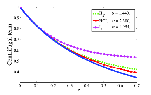
Figure 1: The centrifugal term for different values of $\alpha$ versus the relative distance r.

3 Bound state solutions in three dimensions

Considering only the fluctuation modes, that is the case $\ell=0$, the radial Schrödinger equation has been solved in [47] via Laplace transforms. The more general case $\ell\neq 0$ contains the rotational energies in addition to the vibrational modes, and the corresponding radial Schrödinger equation reduces to Eq.(9). This section shows that by following the procedure of [47], the eigenvalues and eigenfunctions of this case can be obtained via Laplace transforms.

First, a new variable is defined as

$$y=\frac{2\eta}{\alpha}e^{-\alpha r}\,.$$ (11)

By applying this new variable in Eq.(9), the following equation results

$$\left(y^{2}\frac{d^{2}}{dy^{2}}+y\frac{d}{dy}-\frac{1}{4}y^{2}+\frac{\kappa}{2}y-\beta^{2}\right)R_{\ell}(y)=0\,,$$ (12)

where

$$\kappa=\frac{\zeta^{2}}{\eta\alpha}\,,\,\,\,\beta=\frac{\beta_{1}}{\alpha}\,.$$ (13)

In order to have finite solutions at the limit $y\rightarrow\infty$, one should take the following ansatz

$$R_{\ell}(y)=y^{-\beta}\psi_{\ell}(y)\,,$$ (14)

which transforms Eq.(12) into

$$\left(y\frac{d^{2}}{dy^{2}}-(2\beta-1)\frac{d}{dy}-\frac{1}{4}y+\frac{\kappa}{2}\right)\psi_{\ell}(y)=0\,.$$ (15)

The last equation is the same as the one that has already been obtained in [47] for the case $\ell=0$. But by appropriate transformations this can be applied to the case $\ell\neq 0$. Hence by following the same procedure, the solutions of Eq.(15) can be found via Laplace transforms. By applying Laplace transform $F(s)=\mathcal{L}(\psi)$$=\int_{0}^{\infty}e^{-sy}\psi_{\ell}(y)dy$, [42], to Eq.(15), the following equation can be obtained

$$\left(s^{2}-\frac{1}{4}\right)\frac{d}{ds}F(s)+\left[(2\beta+1)s-\frac{\kappa}{2}\right]F(s)=0\,,$$ (16)

which is a first order differential equation and its solutions are in the form

$$F(s)=N\left(s+\frac{1}{2}\right)^{-(2\beta+1)}\left(1-\frac{1}{s+\frac{1}{2}}\right)^{[\kappa-(2\beta+1)]/2}\,,$$ (17)

where $N$ is a constant. Here $\left(1-\frac{1}{s+\frac{1}{2}}\right)^{\kappa-(2\beta+1)}$ is a multi-valued function. In order to have a single valued wave function we impose the condition

$$\kappa-(2\beta+1)=2n,\,\,\,\,n=0,1,2,3,...\,.$$ (18)

Now considering Eq.(10), Eq.(13) and Eq.(18), the eigenvalues of the bound states can be obtained as

$$E_{nl}=\frac{\hbar^{2}}{2mr_{0}^{2}}\left[\ell(\ell+1)C_{0}-\alpha^{2}\left(n+\frac{1}{2}-\frac{\zeta^{2}}{2\eta\alpha}\right)^{2}\right]\,,$$ (19)

where the parameters $\zeta$, $\eta$ are given by Eq.(10). This bound state energy spectrum is the same as the spectrum obtained in [40] by using Nikiforov-Uvarov approach. Also for $\ell=0$ this eigenvalue relation is reduced to the relation obtained in [47].

In order to find the eigenfunctions, we should apply inverse Laplace transforms to Eq.(17). However to do so, it needs to be expanded in power series. Following the method of [47] the normalized eigenfunctions can be achieved as

$$R_{\ell n}(y)=N_{n}y^{\frac{\kappa}{2}-(n+\frac{1}{2})}e^{-y/2}L_{n}^{\kappa-2n-1}(y)\,.$$ (20)

$L_{n}^{\beta}$ are generalized Laguerre polynomials and $N_{n}$ is given by

$$N_{n}=\left[\frac{\alpha n!(\kappa-2n-1)}{\textsf{r}_{0}\Gamma(\kappa-n)}\right]^{1/2}.$$ (21)

The proposed solutions are based on the Perkeris approximation and their validity related to the magnitude of the quantum number $\ell$. Let us now make a comparison between the calculated eigenvalues Eq.(19) and the results of the two-point quasi-rational approximation method [28, 29]. This method is an extension of Padé procedure and is reliable even for high rotational and vibrational quantum numbers. This comparison is made via Fig.(2) for three vibrational levels $n=0$, $n=1$ and $n=2$ of $H_{2}$ molecule. In this figure the solid line shows the eigenvalues obtained from Eq.(19) with $\alpha=1.4405$, $\frac{\hbar^{2}}{2m\textsf{r}_{0}^{2}}=7.5416\times 10^{-3}ev$ and $D=4.7446\,ev$. The dashed lines present the eigenvalues obtained from [29]. It is evident from the figure that there is a noticeable concurrence between two methods approximately for $\ell\leq 24$. By increasing the vibrational quantum number $n$, the coincidence is elongated to smaller values of $\ell$. Specifically the coincidence for $n=0$, $n=1$ and $n=2$ can be seen up to $\ell=28$, $\ell=26$ and $\ell=24$, respectively. Fig.(1) also demonstrates that the worse concurrence occurs for $I_{2}$ molecule, while a better concurrence is resulted for HC1 molecule.

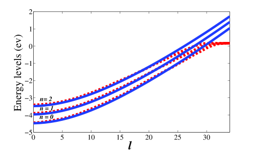
Figure 2: Energy eigenvalues versus rotational quantum number $\ell$.

4 Bound state solutions in $N$ dimensions

The procedure of the preceding section for solving the schrodinger equation with the Morse potential, can be generalized to any given arbitrary dimension $N$. The time independent Schrödinger equation in $N$ dimension can be written as follows

$$\frac{-\hbar^{2}}{2m}\nabla_{N}^{2}\psi(\textbf{{r}})=\left[E-V(\textbf{{r}})\right]\psi(\textbf{r})$$ (22)

where $V(\textbf{{r}})$ is an arbitrary potential. In the presence of a spherical symmetry potential, the wave equation Eq.(22) is known to be separable and can be written as follows, [51]-[54]

$$\psi(\textbf{r})=\textsf{r}^{-(N-1)/2}R_{\ell}(\textsf{r})Y_{\ell_{N-2},...\ell_{1}}^{\ell}(\hat{\textbf{{r}}})$$ (23)

where $Y_{\ell_{N-2},...\ell_{1}}^{\ell}(\hat{\textbf{{r}}})$ are generalized spherical harmonics. Here $\hat{\textbf{{r}}}$ is the unite vector in $N$ dimension and is supposed to be characterized with $(N-1)$ angular coordinates. Using Eq.(23) in Eq.(22), the Schrödinger equation for the radial part $R_{\ell}(\textsf{r})$ becomes

$$\frac{-\hbar^{2}}{2m}\left[\frac{d^{2}}{d\textsf{r}^{2}}-\frac{\lambda^{2}-\frac{1}{4}}{\textsf{r}^{2}}\right]R_{\lambda}(\textsf{r})=[E_{\lambda}-V(\textsf{r})]R_{\lambda}(\textsf{r})$$ (24)

where

$$\lambda=\ell-1+\frac{N}{2}\,.$$ (25)

Applying the Morse potential, Eq.(24) takes the following form

$$\left\{\frac{d^{2}}{dr^{2}}-\frac{\lambda^{2}-\frac{1}{4}}{(r+1)^{2}}-\frac{2m}{\hbar^{2}}\textsf{r}_{0}^{2}\left[D(e^{-2\alpha r}-2e^{-\alpha r})-E_{\lambda}\right]\right\}R_{\lambda}(r)=0$$ (26)

where the variable $r$ is defined in Eq.(5). Using expansion (7) with definitions (8), Eq.(26) can be written as

$$\left(\frac{d^{2}}{dr^{2}}-\eta_{N}^{2}e^{-2\alpha r}+2\zeta_{N}^{2}e^{-\alpha r}-\beta_{1N}^{2}\right)R_{\lambda}(r)=0\,.$$ (27)

Here the parameters $\eta_{N}$, $\zeta_{N}$ and $\beta_{1N}$ are analogue to respectively $\eta$, $\zeta$ and $\beta$ defined in three dimensional case in Eq.(10), and are given as follows

$$\beta_{1N}^{2}=-\frac{2m\textsf{r}_{0}^{2}}{\hbar^{2}}E_{\lambda}+(\lambda^{2}-\frac{1}{4})C_{0}$$  ,

 ,

 .

(28)

The form of Eq.(27) is exactly similar to Eq.(9) and Hence the solutions of the former equation can be obtained via the method of the latter one. Following the procedure of the last section the bound state energy spectrum can be found as

$$E_{n\lambda}=\frac{\hbar^{2}}{2mr_{0}^{2}}\left[\left(\lambda^{2}+\frac{1}{4}\right)C_{0}-\alpha^{2}\left(n+\frac{1}{2}-\frac{\zeta_{N}^{2}}{2\eta_{N}\alpha}\right)^{2}\right]\,,$$ (29)

with

$$n=0,1,2,3,...\,.$$ (30)

Also the corresponding normalized wave functions can be obtained as

$$R_{\lambda n}(y)=N_{n}y^{\frac{\kappa_{N}}{2}-(n+\frac{1}{2})}e^{-y/2}L_{n}^{\kappa_{N}-2n-1}(y)\,.$$ (31)

Here the parameter $\kappa_{N}=\frac{\zeta_{N}^{2}}{\eta_{N}\alpha}$ and $y=\frac{2\eta_{N}}{\alpha}e^{-\alpha r}$ and $L_{n}^{\beta}$ are generalized Laguerre polynomials. Considering Eq.(23) the normalization condition is given as $\int\frac{1}{\alpha y}|R_{\lambda n}(y)|^{2}dy=1$. Applying this normalization condition and using the integrals of Laguerre polynomials, the normalization constant $N_{n}$ can be found as follow

$$N_{n}=\left[\frac{\alpha n!(\kappa_{N}-2n-1)}{\textsf{r}_{0}\Gamma(\kappa_{N}-n)}\right]^{1/2}.$$ (32)

As an example Fig.(3) shows the solutions for eigenfunctions and eigenvalues in seven dimension.

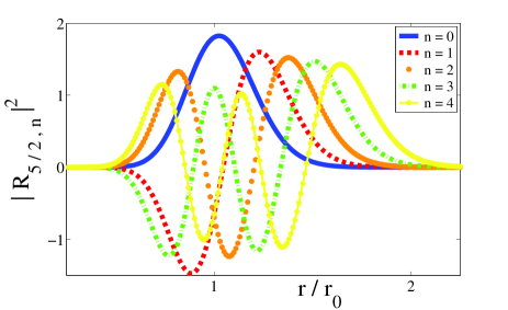
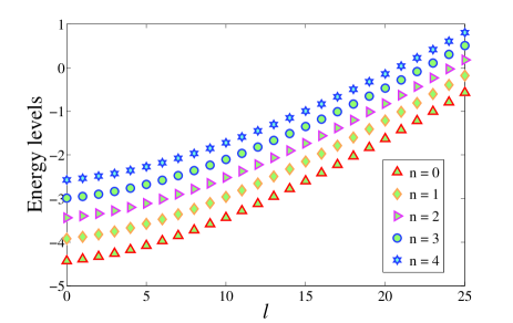
Figure 3: The eigenvalues and eigenfunctions solutions in seven dimensions for hydrogen atom and with $\ell=0$ and $\lambda=5/2$.

5 Conclusions

This study has found an analytical solution for the energy spectrum and wave functions of the Morse problem in arbitrary dimension based on the Pekeris approximation and following [47], by using the Laplace transforms. The obtained solutions in three dimensions are exactly coincides with the results of [40] which are attained by Nikiforov-Uvarov approach. This paper shows that the results can be justified by comparing the calculated energy spectrum with those obtained via the two-point quasi-rational approximation method. This comparison in fact was undertaken to validate the Pekeris approximation which is the basis of the proposed procedure. Nevertheless, the results show that this approximation is not valid for high values of quantum numbers $n$ and $\ell$ except at very low separation distances. Despite this fact the procedure represented in this paper is effective and succinct in its approach, and does not have the complexities of parallel methods. Finally, this method can be generalized in order to include higher dimensions of space.

References

- [1] C. D. Yang, Chaos Soliton. Fract., 37 (2008) 962.
- [2] H. Haken and H. C. Wolf, Molecular Physics and Elements of Quantum Chemistry: Introduction to Experiments and Theory, Springer, Berlin, 1995.
- [3] C. Frankenberg, J. F. Meiring, M. van Weele, U. Platt and T. Wagner, Science 308 (2005) 1010.
- [4] P. M. Morse, Phys. Rev. 34 (1929) 57.
- [5] S. Flügge, Practical Quantum Mechanics, Springer, Berlin, 1974.
- [6] S. M. Ikhdair and R. Sever, Appl. Math. Comput. 218 (2012) 10082.
- [7] C. L. Pekeris, Phys. Rev. 45 (1934) 98.
- [8] L. Infeld and T. E. Hull, Rev. Mod. Phys. 23 (1951) 21.
- [9] A. B. Balentekin, Phys. Rev. A 57(1998) 4188.
- [10] S. H. Dong, R. Lemus and A. Frank, Int. J. Quantum Chem. 86 (2002) 433.
- [11] C. Grosche, J. Phys. A-Math. Gen. 28(1995) 5889.
- [12] C. Grosche, J. Phys. A-Math. Gen. 29 (1996) 365.
- [13] N. Kandirmaz and R. Sever, Chin. J. Phys. 47(1)(2009) 46.
- [14] F. Cooper, A. Khare and U. Sukhatme, Phys. Rep. 251 (1995) 267.
- [15] M. G. Benedict and B. Molnár, Phys. Rev. A 60 (1999) 1737.
- [16] E. D. Filho and R. M. Ricotta, Phys. Lett. A 269 (2000) 269.
- [17] F. R. Silva and E. D. Filho, J. Chem. Phys. Lett. 498 (2010) 198.
- [18] Y. Grandati, Phys. Lett. A 376 (2012) 2866.
- [19] B. Bagchi, P. S. Gorain and C. Quesne, Mod. Phys. Lett. A 21 (2006) 2703.
- [20] G. F. Wei and S. H. Dong, Europhys. Lett. 87 (4) (2009) 40004.
- [21] S. A. Yahiaoui, S. Hattou and M. Bentaiba, Ann. Phys. 322 (2007) 2733
- [22] I. L. Cooper, J. Phys. A-Math Gen. 26 (1993) 1601.
- [23] I. L. Cooper and R. K. Gupta, Phys. Rev. A 52 (1995) 941.
- [24] Z. H. Geng, Y. Dai and S. L. Ding, J. Chem. Phys. 278 (2002) 119.
- [25] J. Yu, S. H. Dong and G. H. Sun, Phys. Lett. A 322 (2004) 290.
- [26] S. H. Dong and G. H. Sun, Phys. Lett. A 314 (2003) 261.
- [27] A. J. Zakrzewski, Comput. Phys. Commun. 175 (2006) 397.
- [28] E. Castro, J. L. Paz and P. Martin, J. Mol. Struc-Theochem 769 (2006) 15.
- [29] E. Castro, P. Martin and J. L. Paz, Phys. Lett. A 364 (2007) 135.
- [30] C. H. Lai, J. Math. Phys. 28 (1987) 1801.
- [31] S. Atag, Phys. Rev. A 37 (1988) 2280.
- [32] T. D. Imbo and U. P. Sukhatme, Phys. Rev. Lett. 54 (1985) 2184.
- [33] M. Bag, M. M. Panja and R. Dutt, Phys. Rev. A 46 (1992) 6059.
- [34] Y. Ou, Z. Cao and Q. Shen, Phys. Lett. A 318 (2003) 36.
- [35] H. Sun, Phys. Lett. A 338 (2005) 309.
- [36] I. Nasser, M. S. Abdelmonem , H. Bahlouli and A. D. Alhaidari, J. Phys. B-At. Mol. Opt. 40 (2007) 4245.
- [37] H. Ciftci, R. L. Hall and N. Saad, J. Phys. A-Math. Gen. 36 (2003) 11807.
- [38] H. Ciftci, R. L. Hall and N. Saad, J. Phys. A-Math. Gen. 38 (2005) 1147.
- [39] O. Bayrak and I. Boztosun, J. Mol. Struc-Theochem 802 (2007) 17.
- [40] C. Berkdemir and J. Han, J. Chem. Phys. Lett. 409 (2005) 203.
- [41] S. M. Ikhdair, J. Chem. Phys. 361 (2009) 9.
- [42] E. Kreyszing, Advanced Engineering Mathematics, John Wiley and Sons, 1979.
- [43] E. Schrödinger, Ann. Phys. 384 (1926) 361.
- [44] M. J. Englefield, J. Austral. Math. Soc. 8 (1968) 557.
- [45] M. J. Englefield, J. Math. Anal. and Appl. 48 (1974) 270.
- [46] R. A. Swainson and G. W. F. Drake, J. Phys. A-Math. Gen. 24 (1991) 79.
- [47] G. Chen, phys. Lett. A 326 (2004) 55.
- [48] G. Chen, Chin. Phys. 14 (6) (2005) 1075.
- [49] A. Arda and R. Sever, J. Math. Chem. 50 (2012) 971.
- [50] D. R. M. Pimentel and A. S. de Castro, Eur. J. Phys. 34 (2013) 199.
- [51] M. M. Nieto, Phys. Lett. A 293 (2002) 10.
- [52] G. Chen, Phys. Lett. A 329 (2004) 22.
- [53] G. Chen and Z. D. Chen, Phys. Lett. A 331 (2004) 312.
- [54] H. Hassanabadi, M. Hamzavi, S. Zarrinkamar and A. A. Rajabi, Int. J. Phy. Sci. 6 (3) (2011) 583.