Algorithms for Brownian dynamics across discontinuities

Abstract

The problem of mass diffusion in layered systems has relevance to applications in different scientific disciplines, e.g., chemistry, material science, soil science, and biomedical engineering. The mathematical challenge in these type of model systems is to match the solutions of the time-dependent diffusion equation in each layer, such that the boundary conditions at the interfaces between them are satisfied. As the number of layers increases, the solutions may become increasingly complicated. Here, we describe an alternative computational approach to multi-layer diffusion problems, which is based on the description of the overdamped Brownian motion of particles via the underdamped Langevin equation. In this approach, the probability distribution function is computed from the statistics of an ensemble of independent single particle trajectories. To allow for simulations of Langevin dynamics in layered systems, the numerical integrator must be supplemented with algorithms for the transitions across the discontinuous interfaces. Algorithms for three common types of discontinuities are presented: (i) A discontinuity in the friction coefficient, (ii) a semi-permeable membrane, and (iii) a step-function chemical potential. The general case of an interface where all three discontinuities are present (Kedem-Katchalsky boundary) is also discussed. We demonstrate the validity and accuracy of the derived algorithms by considering a simple two-layer model system and comparing the Langevin dynamics statistics with analytical solutions and alternative computational results.

Keywords: Diffusion equation, Interface boundary conditions, Layered-inhomogeneous systems, Langevin dynamics

1 Introduction

Brownian motion of particles and molecules in inhomogeneous media can be described by a diffusion equation for the probability distribution function (PDF), $p(\vec{r},t)$, at coordinate $\vec{r}$ and time $t$ [1]:

$$\frac{\partial p(\vec{r},t)}{\partial t}=\vec{\nabla}\cdot\left[D(\vec{r})\vec{\nabla}p(\vec{r},t)-\frac{D(\vec{r})}{k_{B}T}\vec{f}(\vec{r})p(\vec{r},t)\right],$$ (1.1)

where $k_{B}$ is Boltzmann’s constant, and $T$ is the temperature which is assumed to be uniform throughout the system. In Eq. (1.1), $D(\vec{r})$ denotes the coordinate-dependent diffusion coefficient, while $f(\vec{r})$ is the total regular force (i.e., excluding random molecular collisions that cause the diffusive dynamics) acting on the Brownian particle. Obviously, a continuous position-dependent $D(\vec{r})$ can only be defined if the diffusion coefficient does not exhibit strong variations on length scales of the order of the particle’s size. A simple example where this criterion is not met, is the case of a colloidal particle of size $R_{c}\sim 10-10^{3}$ nm intersecting a thin interface, of the size of a single molecular layer, between immiscible fluids such as water and oil. Typically, the oil is much more viscous than the water and, thus, the diffusion coefficient of the particle in it is much smaller than on the aqueous side. In general, the solubility of the particle may be very different in the water and oil compartments, implying that it also experiences a force at the interface pulling it toward the medium with a lower chemical potential.

A water-oil interface constitutes an example of a layered system with a sharp, essentially discontinuous, boundary between media with distinct diffusion constants. Within each layer, the PDF can be found by solving the partial differential equation (PDE) (1.1) with a constant $D$, and the transition between the layers is accounted for by introducing appropriate boundary conditions (to be discussed below) that the PDFs in the different layers satisfy. Note that the diffusing particle is assumed to be point-like in this continuum description, which is applicable only to length scales much larger than $R_{c}$. The solutions may be found analytically by, e.g., separation of variables or the Laplace transform method, or numerically through some kind of a discretization scheme, e.g., finite elements, finite differences, and the marker cell method [1, 2, 3, 4, 5, 6, 7, 8, 9, 10, 11, 12, 13, 14, 15]. As the number of layers and boundaries becomes larger, the calculation of $p(\vec{r},t)$ becomes increasingly complicated, which calls for further development of solution methods of diffusion problems in multi-layered systems. In a recent study, we considered the problem of drug release from a drug eluting stent (layer 1) into the artery (layer 2) across a semi-permeable thin membrane (boundary) [16]. We presented a novel approach for finding the time-dependent PDF, which is based on generating a large ensemble of statistically-independent single-particle trajectories using Langevin Dynamics (LD) simulations. In each layer, the trajectory is computed using the statistically-reliable Grønbech-Jensen and Farago (GJF) algorithm [17, 18], which is supplemented with an algorithm describing how to treat a crossing event of the interface between the layers. We found agreement between our computational results and analytical solution of the very same model [19]. Here, we expand our previous work and present a set of such algorithms for crossing different types of commonly encountered boundaries. These include interfaces with (i) a discontinuity in $D$, (ii) a thin semi-permeable membrane, and (iii) an imperfect contact with discontinuity in the chemical potential resulting in a delta-function force. We test each of the algorithms on a simple model system of a particle starting on one side of the interface and spreading across the system (see fig. 1). In cases (i) and (iii) we compare our results with the analytical solution of the problem, and in case (ii) with LD simulations of a similar system that explicitly includes a thin membrane. In all cases, we obtain an excellent fit to the expected solutions. Finally, we consider the case where all three effects are present. Notice that while we study a two-layer system with a single boundary in this paper, the algorithms are applicable to any multi-layer system. In each layer, the trajectory is computed using the GJF integrator for LD, and upon crossing a boundary, the appropriate algorithm is applied. The simulations presented here were performed on commonly available PCs within a modest CPU time of no more than a few hours.

2 Boundary conditions at interfaces

In what follows, we consider mass transport in a class of model systems consisting of two regions with diffusion coefficients $D_{1}$ and $D_{2}$, respectively, and an infinitesimally thin interface separating them at $x=0$. A schematic of such a system is shown in fig. 1. In many application, one is only interested in mass transport in the $x$ direction (the coordinate perpendicular to the interface), which is characterized by the projected PDF, $p(x,t)=\iint dz\!dyp(\vec{r},t)$. If the mass transport process is purely diffusive and the dynamics is not driven by any regular force (i.e., $f(x)=0$ everywhere except, perhaps, at the boundaries), then the PDF in each region, $p_{i}(x,t)$ ($i=1,2$), is governed by

$$\frac{\partial p_{i}}{\partial t}=D_{i}\frac{\partial^{2}p_{i}}{\partial x^{2}}.$$ (2.1)

The PDFs in both regions must be matched at the interface $x=0$, and two boundary conditions (BCs) must be specified. If mass is not lost or generated at the interface (no source or sink), then the probability flux, $J$, must be continuous on the interface for any $t>0$

$$J(0,t)=-D_{1}\frac{\partial p_{1}}{\partial x}=-D_{2}\frac{\partial p_{2}}{\partial x}.$$ (2.2)

The other BC to be specified at $x=0$ depends on the nature of the interface. The transport of material in one of the directions can be completely blocked by placing a perfectly reflecting [$J(0,t)=0$] or perfectly absorbing [$p(0,t)=0$] barriers. Typically, however, we are interested at intermediate situations where neither the probability nor the the flux vanish. More specifically, two types of interfaces are often considered in diffusion controlled setups. The first one is an “imperfect contact” [20] that imposes material partitioning across the boundary such that

$$p_{1}(0,t)=\sigma p_{2}(0,t).$$ (2.3)

where $\sigma$ is known as the partition coefficient of the interface. Note that when $\sigma=1$, the PDF exhibits no discontinuity at the boundary [$p_{1}(0,t)=p_{2}(0,t)$], which is then considered as a “perfect” one. The second commonly imposed BC describes the effect of a thin semi-permeable membrane which, similarly to Eq. (2.3), leads to a discontinuity in the probability. In the case of a semi-permeable thin membrane, the probability jump and the flux are related by [21, 22]

$$J(0,t)=P\left[p_{1}(0,t)-p_{2}(0,t)\right].$$ (2.4)

where $P$ is known as the permeability of the membrane. Note that, when $P\rightarrow\infty$, Eq. (2.4) reduces to the continuity condition: $p_{1}=p_{2}$ (or, otherwise, the flux diverges), while $P\rightarrow 0$ corresponds to a perfectly reflecting boundary ($J=0$).

In the most general case, the particle experiences all three effects (discontinuity in $D$, imperfect contact, and the presence of a membrane) at the interface. In this case, one needs to impose the Kedem-Katchalsky (KK) BC that reads [23, 24]

$$J(0,t)=-D_{1}\frac{\partial p_{1}}{\partial x}=-D_{2}\frac{\partial p_{2}}{\partial x}=P\left[p_{1}(0,t)-\sigma p_{2}(0,t)\right].$$ (2.5)

3 Langevin Dynamics

3.1 Diffusion in homogeneous medium

At the heart of the proposed method for computing the PDF $p(x,t)$ lies the alternative route to Eq. (2.1) for depicting particle diffusion, which is the Langevin equation of motion

$$m\frac{dv}{dt}=-\alpha v+\beta(t)+f(x),$$ (3.1)

where $m$ and $v=dx/dt$ denote, respectively, the mass and velocity of the diffusing particle. Langevin equation describes Newtonian dynamics under the action of (i) a regular force $f(x)$, (ii) a friction force, $-\alpha v$, and (iii) stochastic Gaussian thermal noise chosen from a normal distribution with zero mean, $\langle\beta(t)\rangle=0$ and delta-function auto-correlation $\langle\beta(t)\beta(t^{\prime})\rangle=2k_{B}T\alpha\delta(t-t^{\prime})$. The friction coefficient, $\alpha$, in Langevin equation and the diffusion coefficients, $D$, in the corresponding diffusion equation, satisfy $\alpha D=k_{B}T$, which is Einstein’s relation. Notice that Eq. (2.1) describes a purely diffusive behavior in each layer, which corresponds to the case where the regular force $f(x)=0$ in Eq. (3.1). Nevertheless, we include the regular force term in Langevin’s equation because we need it for reproducing the imperfect contact BC (2.3) - see section 3.5.

The idea is to compute $p(x,t)$ from an ensemble of statistically-independent stochastic particle trajectories of duration $t$. The distribution of $x$ at $t=0$ is drawn from the initial distribution $p(x,0)$. The trajectories $x(t)$ are computed by performing discrete-time integration of Langevin equation (3.1). For this purpose, we use the GJF integrator [17, 18]

$$x^{n+1} = x^{n}+b\,\left[dtv^{n}+\frac{dt^{2}}{2m}f^{n}+\frac{dt}{2m}\beta^{n+1}\right]$$ (3.2)

$$v^{n+1} = a\,v^{n}+\frac{dt}{2m}\left(a\,f^{n}+f^{n+1}\right)+\frac{b}{m}\beta^{n+1},$$ (3.3)

to advance the coordinate $x^{n}=x(t_{n})$ and velocity $v^{n}=v(t_{n})$ by one time step from $t_{n}=n\,dt$ to $t_{n+1}=t_{n}+dt$. In the above GJF equations (3.2)-(3.3), $f^{n}=f(x^{n})$, and $\beta^{n}$ is a Gaussian random number satisfying

$$\langle\beta^{n}\rangle=0\ ;\ \langle\beta^{n}\beta^{l}\rangle=2\alpha k_{B}Tdt\delta_{n,l},$$ (3.4)

and the damping coefficients of the algorithm are

$$b=\displaystyle{1\over 1+\left(\alpha\,dt/2m\right)},\qquad a=b\left[1-\left(\alpha\,dt/2m\right)\right].$$ (3.5)

Generally speaking, numerical integration involves discretization errors which often scale linearly or quadratically with $dt$. The GJF integrator is chosen because of its unusual robustness against such errors, which is critical for achieving accurate statistics of configurational results even when the integration time step $dt$ is not vanishingly small. More specifically, the GJF integrator accomplishes statistical accuracy for configurational sampling of the Boltzmann distribution in closed systems; and it also provides the correct Einstein diffusion, $\langle x^{2}\rangle=2Dt$ (with $D=k_{B}T/\alpha$), of a freely diffusing particle in an unbounded system [17, 18, 25, 26]. Note that on time scales

$$t\ll\tau_{\rm ballistic}=\frac{m}{\alpha},$$ (3.6)

Langevin’s dynamics is predominantly ballistic. In “smooth” systems, the GJF algorithm can be implemented in simulations with relatively large time steps $dt>\tau_{\rm ballistic}$, and still produce accurate statistical results at asymptotically large times. By contrast, in “layered” systems, especially when encountering a discontinuity in $D(x)$ (see section 3.3 below), it is important to perform the simulations in the ballistic regime, i.e., with $dt\ll\tau_{\rm ballistic}$, in order to correctly mimic the imposed BCs at the interfaces between the layers.

3.2 Reflecting and absorbing boundaries

In addition to the interface at $x=0$ shown in fig. 1, the system may be bound by reflecting and absorbing interfaces. These interfaces are treated in the LD simulations as follows: If the particle crosses a reflecting boundary at $x=L$, then its new position and velocity are redefined as follows:

$$x^{n+1}\rightarrow 2L-x^{n+1}\qquad v^{n+1}\rightarrow-v^{n+1},$$ (3.7)

which sets the new position of the “escaping” particle back within the boundaries of the systems and reverse its direction of propagation. Crossing an absorbing boundary is a special case of the imperfect contact BC (2.3) with $\sigma=0$ or $\sigma\rightarrow\infty$ ($1/\sigma=0$), where the PDF vanishes on one side of the interface. The discussion on this type of BC is given on section 3.5.

3.3 Transition between layers with different diffusion coefficients

The problem of moving in a medium with space-dependent diffusion coefficient, $D(x)$, invokes the so-called “Itô-Stratonovich dilemma” [27, 28, 29]. The dilemma refers to the ambiguity regarding the proper value of the diffusion coefficient to be used in discrete-time integration. The correct choice is not a-priory clear because $D(x^{n})\neq D(x^{n+1})$. Dealing with all the aspects of the dilemma is beyond the scope of this work, and we therefore provide here a limited review containing only the information necessary for understanding the algorithm for crossing a sharp interface. For a more detailed discussion on the Itô-Stratonovich dilemma, the reader is referred to our previous works [30, 31]. The problem of diffusion in layered heterogeneous systems discussed in this section has been also treated in the framework of the random walk model [32, 33, 34, 35].

Obviously, it is desirable to run an algorithm that uses the friction coefficient at the beginning of the time-step, $\alpha(x^{n})=k_{B}T/D(x^{n})$. This is known as the Itô-convention [36] and, algorithmically, it is the simplest one since any other convention that also uses $\alpha(x^{n+1})=k_{B}T/D(x^{n+1})$ involves an implicit integration method. However, using Itô’s convention to integrate Eqs. (3.2) and (3.3) would not lead to the correct statistics. More precisely, if the integration is performed with a time step in the diffusive regime $dt\gtrsim\tau_{\rm ballistic}$, a “spurious force” term, $\vec{f}_{s}=-k_{B}T\alpha^{\prime}/\alpha$ must be added to the dynamics [37]. This is not a real physical force (as the name implies) and, thus, it has no influence on the equilibrium distribution to which the PDF relaxes at large times in closed systems. It nevertheless represents a real drifting effect of Brownian particles in the direction of lower friction. Without the spurious force term, the statistics becomes accurate only in the limit when $dt\rightarrow 0$ (i.e., when the time step $dt\ll\tau_{\rm ballistic}$), but the rate of convergence to the continuous-time PDF with $dt$ may be quite slow [30]. This is because the drift which is generated by the spurious force is an inertial effect that takes place at the ballistic regime of the LD [31].

In layered systems, the friction function is a step-function and its derivative is the Dirac delta-function: $\alpha^{\prime}=k_{B}T[1/D_{2}-1/D_{1}]\delta(x)$. This means that the spurious force $\vec{f}_{s}=-k_{B}T\alpha^{\prime}/\alpha$ vanishes everywhere and has a singularity at $x=0$, which raises the question how to treat it in the discrete-time integration. To state it differently, the question is how to reproduce the desired drifting effect at the interface without a spurious force. The solution is to avoid using the Itô convention for choosing the friction coefficient and replace it with a different one. This alternative convention, termed the “ballistic (inertial) convention”, is an explicit one and it yields the correct drifting effect at sharp interfaces (as well as in systems with smooth friction functions) [30, 31, 38]. In layered systems, the algorithm runs as follows:

If $x^{n}$ and $x^{n+1}$ are found on different sides of the interface located at $x=L$, then $x^{n+1}$ and $v^{n+1}$ need to be recalculated as follows:

1. Calculate the ballistic position $x^{n+1}_{b}=x^{n}+v^{n}dt$

2. Calculate the average friction coefficient along the ballistic trajectory

   $$\bar{\alpha}=\frac{\alpha\left(x^{n}\right)\left|x^{n}-L\right|+\alpha\left(x^{n+1}_{b}\right)\left|x^{n+1}_{b}-L\right|}{\left|x^{n}-L\right|+\left|x^{n+1}_{b}-L\right|}$$

3. Advance the trajectory from $(x^{n},v^{n})$ to $(x^{n+1},v^{n+1})$ by one step $dt$, according to Eqs. (3.2)-(3.5), with $\bar{\alpha}$.

Notice that in some rare cases, the new position $x^{n+1}$ will be found on the same size as $x^{n}$, but this is acceptable since small discretization errors are always present when encountering a discontinuity in $D$. Nevertheless, with the above ballistic convention, the rate of convergence to the correct statistics in the limit $dt\rightarrow 0$ is markedly faster than that of the Itô convention and, therefore, one can use much larger time-steps without scarifying the statistical accuracy of the results.

In order to demonstrate the accuracy of the above algorithm, we consider the system depicted in fig. 1 with an interface at $x=0$ and delta-function initial distribution: $p(x,0)=\delta(x-x^{0})$. Assuming (i) continuity of the flux, Eq. (2.2), and (ii) continuity of the probability at a “perfect” contact, Eq. (2.3) with $\sigma=1$, the analytical solution is (for $x^{0}<0$):

$$p(x,t)=\left\{\begin{array}[]{ll}\displaystyle\frac{1}{\sqrt{4\pi D_{1}t}}\exp\left[{-\displaystyle\frac{(x-x^{0})^{2}}{4D_{1}t}}\right]+\displaystyle\frac{A}{\sqrt{4\pi D_{1}t}}\exp\left[{-\displaystyle\displaystyle\frac{(x+x^{0})^{2}}{4D_{1}t}}\right]&x<0\\ &\\ \displaystyle\frac{B}{\sqrt{4\pi D_{2}t}}\exp\left[{-\frac{(x-\tilde{x}^{0})^{2}}{4D_{2}t}}\right]&x>0\ ,\end{array}\right.$$ (3.8)

with

$$\tilde{x}^{0}=x^{0}\sqrt{D_{2}/D_{1}},\qquad A={1-\sqrt{D_{2}/D_{1}}\over 1+\sqrt{D_{2}/D_{1}}},\qquad B={2\over 1+\sqrt{D_{1}/D_{2}}}.$$ (3.9)

Fig. 2 depicts this analytical solution at $t=100$ and $t=500$ (solid red and blue lines, respectively) for $x^{0}=-5$ and

$$D(x)=\left\{\begin{array}[]{ll}1&x<0\\ 0.1&x>0\end{array}\right.,$$ (3.10)

along with the results of LD simulations that are based on $10^{8}$ trajectories. In the simulations, we set $m=1$ and $k_{B}T=1$. Thus, the friction coefficients in the layers are given by $\alpha_{1}=k_{B}T/D_{1}=1$ and $\alpha_{2}=k_{B}T/D_{2}=10$. The integration time step is chosen to be $dt=0.01$, which is an order of magnitude smaller then the ballistic time in the more viscous layer ($\tau_{\rm ballistic}^{x>0}=m/\alpha=1/10$). All the trajectories start at $x^{0}=-5$, and the initial velocity $v^{0}$ is drawn from the equilibrium Maxwell-Boltzmann (MB) distribution

$$\rho_{\rm MB}(v)=\sqrt{\frac{m}{2\pi k_{B}T}}\exp\left(-\frac{mv^{2}}{2k_{B}T}\right).$$ (3.11)

The computational results are marked by circles and exhibit an excellent agreement with the analytical solution (LABEL:eq:2layer). As stated above, discretization errors may be encountered close to the interface, but these are nearly-negligible in fig. 2.

3.4 Transition of a semi-permeable membrane

The transport of material in the system can be controlled by placing a thin membrane with very low diffusivity, which slows down the flow of particles. In the limit when both the membrane diffusion coefficient, $D_{m}$, and width, $h$, vanish, the presence of the membrane can be represented by a boundary satisfying condition (2.4), where $P=D_{m}/h$ is the permeability, or the mass transfer coefficient, of the membrane [22]. Importantly, the material flux is assumed to be continuous across the boundary, which means that the limits $D_{m}\rightarrow 0$ and $h\rightarrow 0$ are taken such that the amount of material which is trapped inside the membrane is negligible. This is to be expected because the typical diffusion time of particles inside the membrane, $\tau_{m}\sim h^{2}/D_{m}=h/P\rightarrow 0$, for any non-vanishing value of $P$.

In LD simulations, the mass flux BC (2.4) can be implemented by a simple transition rule that the trajectory crosses the boundary with probability $\Pi$, and is reflected from it with the complementary probability $1-\Pi$. In the case of a reflection, Eq. (3.7) is used for calculating the coordinate and velocity after the time-step. In order to find the relationship between the transition probability of the simulations, $\Pi$, and the membrane permeability, $P$, we begin with the following standard derivation of Fick’s first law [39]. Let us denote by $J(x)$ the net probability flux crossing an imaginary interface at $x$. The net flux is the difference between the probability flux associated with particles moving from left to right in the positive direction, and the negative flux associated with particles moving from right to left: $J=J^{+}-J^{-}$. The positive flux, $J^{+}(x)$, can be written as the product of the average thermal velocity, $v_{\rm th}$, of particles moving rightward (i.e., particles with $v>0$) and half the density of particles located slightly left to $x$ (which is where these particles are coming from):

$$J^{+}(x)=\frac{1}{2}p\left(x-\frac{l}{2}\right)v_{\rm th}\simeq\frac{v_{\rm th}}{2}\left[p(x)-\frac{l}{2}\frac{\partial p}{\partial x}\right].$$ (3.12)

In the above equation, the density of particles residing left to $x$ is evaluated at $x-l/2$ ($l>0$). The relationship between $l$ and the other system parameters will be determined later [see Eq. (3.16)]. The following should be also noted about Eq.(3.12): (i) The factor half arises from the physical assumption that the ensemble of particles is found at thermal equilibrium. Strictly speaking, this assumption is valid only in the overdamped limit considered by Fick’s law, when the velocity relaxation after crossing a barrier is (almost) instantaneous, i.e., the limit $\tau_{\rm ballistic}\rightarrow 0$. Specifically, at each point, the velocity distribution function of the particles is the Maxwell-Boltzmann (MB) one (3.11), which means that only half of the particles residing left to $x$ are moving in the right direction. (ii) From the MB distribution function we find that the average thermal velocity of those particles is

$$v_{\rm th}=2\int_{0}^{\infty}v\rho_{\rm MB}(v)dx=\sqrt{\frac{2k_{B}T}{\pi m}},$$ (3.13)

where the factor 2 here is due to the fact that the average is taken only over half of the population of particles. Similarly to Eq.(3.12),

$$J^{-}(x)=\frac{1}{2}p\left(x+\frac{d}{2}\right)v_{\rm th}\simeq\frac{v_{\rm th}}{2}\left[p(x)+\frac{l}{2}\frac{\partial p}{\partial x}\right].$$ (3.14)

The net flux is then

$$J(x)=J^{+}(x)-J^{-}(x)=-\frac{v_{\rm th}l}{2}\frac{\partial p}{\partial x},$$ (3.15)

and by comparison with Fick’s first law, we identify that

$$l=\frac{2D}{v_{\rm th}}.$$ (3.16)

The length $l$ is often identified as the “mean free path” (MFP) of the particles [39]. This is essentially the characteristic distance that the particle travels before encountering a random collision and acquiring a new random velocity. In the Langevin equation formalism, this is associated with the characteristic ballistic distance of the dynamics. Indeed, the mean free travel time can be estimates by $\tau_{\rm free\ path}=l/v_{\rm th}=\pi(mD/k_{B}T)=\pi(m/\alpha)=\pi\tau_{\rm ballistic}$, which up to a factor of $\pi$ coincides with the ballistic time defined in Eq. (3.6).

Let us assume that we have a barrier at $x=L$ with (symmetric) crossing and reflection probabilities $\Pi$ and $1-\Pi$, respectively. For simplicity, let us assume that the diffusion coefficients on both sides are the same. (We could continue the derivation without this assumption). Let us denote by $J_{1}^{+}=J_{1}^{\rm in}$ and $J_{2}^{-}=J_{2}^{\rm in}$ the probability fluxes incoming to the interface from the left and right sides, respectively. The outgoing currents are given by $J_{1}^{-}=(1-\Pi)J_{1}^{\rm in}+\Pi J_{2}^{\rm in}$ and $J_{2}^{+}=(1-\Pi)J_{2}^{\rm in}+\Pi J_{1}^{\rm in}$, which means that the net fluxes, $J_{1}=J_{1}^{+}-J_{1}^{-}$ and $J_{2}=J_{2}^{+}-J_{2}^{-}$, are

$$J_{1}=J_{2}=\Pi\left(J_{1}^{in}-J_{2}^{in}\right).$$ (3.17)

The fact that the fluxes on both sides of the barrier are equal to each other is not surprising since particles can only cross or be reflected from the barrier, but not to be eliminated or generated. Now, from Eq. (3.12) we have that

$$J_{1}^{\rm in}=(v_{\rm th}/2)\cdot p_{1}(L-l/2)\simeq(v_{\rm th}/2)[p_{1}(L)-(l/2)\partial p_{1}/\partial x]$$

where $p_{1}(L)$ is the probability density on the left side of the barrier. Similarly, from Eq. (3.14), we get

$$J_{2}^{\rm in}=(v_{\rm th}/2)\cdot p_{2}(L+l/2)\simeq(v_{\rm th}/2)[p_{2}(L)+(l/2)\partial p_{2}/\partial x],$$

where $p_{2}(L)$ is the probability density on the right side. By subtracting the above expressions, we find that

$$J_{1}^{\rm in}-J_{2}^{\rm in}=\frac{v_{\rm th}}{2}[p_{1}(L)-p_{2}(L)]-\frac{v_{\rm th}l}{4}\left[\frac{\partial p_{1}}{\partial x}+\frac{\partial p_{2}}{\partial x}\right].$$ (3.18)

From Eq. (3.15) and the fact that the net fluxes on both sides are the same, we conclude that the second term on the r.h.s. of Eq.(3.18) is equal to the $J$ at the interface. Also, from Eq. (3.17) we conclude that the term on the l.h.s. of Eq. (3.18) is equal to $J/\Pi$. Thus, Eq. (3.18) can be also written as $J/\Pi=(v_{\rm th}/2)[p_{1}(L)-p_{2}(L)]+J$, which leads to

$$J=\frac{v_{\rm th}\Pi}{2(1-\Pi)}[p_{1}(L)-p_{2}(L)].$$

This equation has the form of Eq. (2.4) (which is written for a membrane located at $L=0$) and we, thus, arrive at the relationship between the membrane mass transfer coefficient and the crossing probability in the LD simulations: $P=\displaystyle{v_{\rm th}\,\Pi\over 2(1-\Pi)}$, or

$$\Pi=\frac{2P}{2P+v_{\rm th}},$$ (3.19)

where $v_{\rm th}$ is given by Eq. (3.13).

We notice from Eqs. (3.19) and (3.13) that the transition probability $\Pi$ in the LD simulations is a function of the mass of the particle $m$. This feature of the algorithm is nicely demonstrated in fig. 3, showing the PDF computed at (a) $t=100$ and (b) $t=500$ in the setup shown in fig. 1 with a semi-permeable boundary at $x=0$. As in the example presented in fig. 2, we assume a delta-function initial distribution $p(x,0)=\delta(x-x^{0})$ with $x^{0}=-5$, but in contrast to fig. 2, we here set $D_{1}=D_{2}=1$ as we want to “separate” the semi-permeable membrane effect from the impact of the discontinuity in $D$. The decision whether the trajectory crosses the interface is done a-la Monte Carlo, i.e., by drawing a random number ${\cal R}$ uniformly distributed between 0 and 1, and allowing crossing if ${\cal R}\leq\Pi$. The black circles depict the results from simulations with $m=1$ and $P=v_{\rm th}/8$, in which case $\Pi=1/5$. The red squares represent the results of simulations with $m^{*}=4$ at the same temperature ($k_{B}T=1$), which means that $v_{\rm th}^{*}=v_{\rm th}/2$. Since now $P=v_{\rm th}/8=v_{\rm th}^{*}/4$, the crossing probability in the simulations is now set to $\Pi=2P/(2P+v_{\rm th}^{*})=1/3$, yielding results that are almost indistinguishable from those obtained in the simulations with $m=1$ and $\Pi=1/5$.

Unfortunately, the two-layer problem with a semi-permeable membrane and delta-function initial conditions cannot be solved analytically and presented in the same form as in Eq. (LABEL:eq:2layer). Therefore, in order to validate the algorithm, we performed another set of LD simulations where, rather than using a boundary with crossing probability $\Pi$, we explicitly introduced a thin membrane, of width $h=0.05$, in the interval $|x|<h/2$. The simulations with the explicit presence of a membrane were performed according to the algorithm presented in section 3.3 for Langevin simulations with discontinuous diffusion coefficient. We set $D=1$ for $|x|>h/2$ (i.e., in both layers) and $D_{m}=Ph=v_{\rm th}h/8$ in the thin membrane, in order to match it with the simulations results described in the previous paragraph and depicted by black circles in fig. 3 for $m=1$ and $k_{B}T=1$. We thus set $D_{m}=h(2k_{B}T/\pi m)^{0.5}\simeq 0.005$ or $\alpha_{m}=k_{B}T/D_{m}\simeq 200$, which requires the simulations to be performed with a very small time step, $dt=0.001$, which is smaller than the ballistic time in the thin membrane ($\tau_{\rm ballistic,m}=m/D_{m}=0.005$). The bound imposed on the simulation time step by the large friction coefficient of the membrane explains the utility of the above semi-permeable boundary algorithm, where much larger time steps can be used. Moreover, one also needs to account for the (small, yet non-negligible) fraction of particles that are trapped in the membrane, which is done by excluding from the statistics the trajectories where $|x|<h/2$ at the moment of the measurement. The results of the explicit-membrane simulations are presented with blue triangles in fig. 3. The agreement with the semi-permeable boundary algorithm simulations (black circles and red squares) is excellent, which proves the validity and accuracy of the algorithm.

3.5 Transition of an imperfect contact boundary

A non-perfect contact interface is a barrier that maintains a fixed ratio $\sigma$ between the probability densities on both sides, see Eq. (2.3). This BC is essentially a detailed-balance condition. In a two-layer closed system with no external potential, equilibrium is achieved when the density in each layer is uniform, and the ratio between them is

$$\sigma=\frac{p_{1}}{p_{2}}=\exp\left(-\frac{\Delta\mu}{k_{B}T}\right)$$

where $\Delta\mu=\mu_{2}-\mu_{1}$ is the chemical potential difference between the layers. The step-function chemical potential,

$$\mu_{\rm step}(x)=\Delta\mu H(x-L)$$ (3.20)

[where $H$ is the Heaviside function], produces a delta-function force at $x=L$, the position of the imperfect contact interface. This resembles the case discussed in section 3.3 where a delta-function force has also been encountered; however, the difference is that here we deal with a real physical, not a spurious, singular force. The question, again, is how to account for such a force that vanishes everywhere. A plausible algorithm would be to resort to energy considerations, and check whether the particle has enough kinetic energy to cross the interface between the layers. Thus, if the particle arrives from the thermodynamically less favorable medium with higher chemical potential then its allowed to cross the interface, but if it arrives from the opposite side then it makes the transition only if it has enough kinetic energy to overcome the potential barrier: $m(v^{n})^{2}/2\geq|\Delta\mu|$. The velocity of the particle after the transition is determined by energy conservation: $(v^{n})^{2}+2m\mu(x^{n})=(v^{n+1})^{2}+2m\mu(x^{n+1})$. If the particle arrives from the lower chemical potential side and has no sufficient energy to cross the barrier then it is reflected backward, and the algorithm for a reflecting boundary, see Eq. (3.7), is applied.

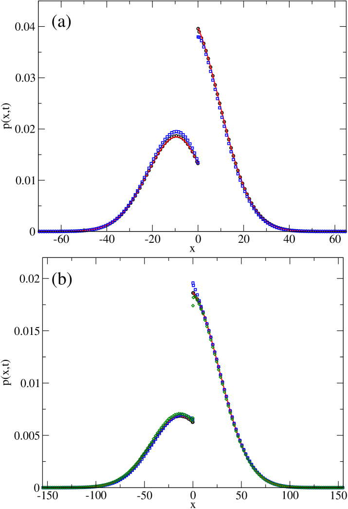
Figure 4: (a) The PDF, $p(x,t)$, in a two-layer system with an imperfect contact with partition coefficient $\sigma=1/3$ at $x=0$, at time $t=100$. The initial position of the particle is at $x^{0}=-5$. The black circles show the simulation results, while the red solid line show the analytical solution Eq. (LABEL:eq:2layer) with the coefficient $A$ and $B$ given by Eq. (3.21). The blue squares depict the simulation results that are based on the (incorrect) algorithm utilizing energy considerations at the interface. (b) Black circles and red solid line - same as (a) at $t=500$. The blue squares and green diamonds depict results obtained when the region over which the chemical potential changes is 10 time wider than in Eq. (3.22) - blue squares, and $10^{-2}$ thinner than in Eq. (3.22) - green diamonds.

One may expect that the above algorithm for crossing a step-function energy barrier would reproduce the desired PDF when the time step is sufficiently small, i.e., for $dt\ll\tau_{\rm ballistic}$. This turns out not to be the case, as demonstrated in fig. 4 (a) that shows results from simulations of the two-layer model system in fig. 1 with an imperfect contact surface at $x=0$. The partition coefficient of the imperfect contact boundary is set to $\sigma=1/3$. As in the examples studied in previous sections, we compute the PDF at $t=100$ from $10^{8}$ independent trajectories, all starting at $x^{0}=-5$. As in section 3.4, we set $D_{1}=D_{2}=1$. The blue squares depict the results of LD simulations of the above algorithm, while the solid red line shows the analytical solution, which takes the same form as in Eq. (LABEL:eq:2layer), with

$$A={\sigma-1\over\sigma+1}\qquad B={2\over\sigma+1}.$$ (3.21)

We observe that the computational results depart from the the analytical solution and do not achieve the correct ratio $\sigma$ between the densities on both sides of the interface.

The failure of the above algorithm to yield correct results is rooted in the lack of detailed-balance between the fluxes crossing the interface in both directions. If the velocity follows the Maxwell-Boltzmann distribution (3.11), then the above algorithm transfers a fraction 1 of the particles that fall down the potential gap, and a fraction $\sigma<1$ (or $1/\sigma$, for $\sigma>1$) of the particles that climb from the lower to the higher potential side. This, however, is not sufficient to ensure detailed-balance if the system has not reached a steady-state yet. To preserve the ratio $\sigma$ between the densities on both side of the interface for any time $t$, the algorithm must also produce the correct fluxes incoming to the interface from both sides. This, however, cannot be achieved by the above algorithm that, irrespective of $\sigma$, yields the same first crossing time statistics. In the limit $\sigma\rightarrow\infty$, for instance, we deal with a one-sided barrier, and from Eq. (2.3) we expect $p_{1}(0)=0$. But with the above algorithm $p_{1}(0)$ does not vanish because, at any time $t$, there is a fraction of “surviving” trajectories reaching arbitrarily close to the surface.

The above argument suggests that the interface at $x=L$ must also have influence on nearby particles, even on those who have never reached it. This can be accomplished by replacing the step-function potential energy Eq. (3.20) with the following sharp piece-wise linear continuous function:

$$\mu_{\rm linear}(x)=\left\{\begin{array}[]{ll}\displaystyle 0&x<L-\frac{l_{1}}{2}\\ \displaystyle\frac{\Delta\mu}{2}\left(\frac{x-L+l_{1}/2}{l_{1}/2}\right)&L-\frac{l_{1}}{2}<x<L\\ \displaystyle\frac{\Delta\mu}{2}\left(1+\frac{x-L}{l_{2}/2}\right)&L<x<L+\frac{l_{2}}{2}\\ \displaystyle\Delta\mu&x>L+\frac{l_{2}}{2},\end{array}\right.$$ (3.22)

where $l_{i}$ ($i=1,2$) is the mean free path (MFP) in each layer [see Eqs. (3.16) and (3.13)]. The piece-wise linear potential (3.22) introduces a force, $f(x)=-d\mu_{\rm linear}(x)/dx$, in a interface layer (IL) region of the size of the (average) MPF $(l_{1}+l_{2})/2$, around the interface. As the MPF is comparable to the the ballistic distance (see discussion above, section 3.4), the GJF equations (3.2)-(3.3) must be iterated with a sufficiently small time-step $dt\ll\tau_{\rm ballistic}$ in order to ensure that the trajectory passes through the IL and the force is felt by the particle. The resulting statistics must then be corrected to account for the distortion of the step-function potentials energy. This is done by multiplying the computed PDF with an exponential weight function associated with the Boltzmann factors of the “step” and “linear” potentials

$$w(x,t)_{\rm step}=p(x,t)_{\rm linear}\cdot\exp\left[\frac{\mu_{\rm linear}(x)-\mu_{\rm step}(x)}{k_{B}T}\right],$$ (3.23)

and then normalizing the result

$$p(x,t)=\frac{w(x,t)_{\rm step}}{\int_{-\infty}^{\infty}w(x,t)_{\rm step}\,dx}.$$

The results derived based on this algorithm are presented by black circles in fig. 4 (a). They exhibit excellent agreement with the analytical solution which is plotted in red solid curve.

The width of the IL where the piece-wise linear potential (3.22) changes, has been set to $\Delta=(l_{1}+l_{2})/2$ - the average MFP. This choice is obviously not unique and, depending on the system in question, may be altered in order to improve the accuracy of the results and the computational speed of the algorithm. The influence of the IL thickness on the results is demonstrated in fig. 4 (b) showing the PDF at $t=500$ for the same system as in (a). The black circles and red solid line show the computational results and the analytical solution and, as in fig. 4 (a), we observe an excellent agreement between them. The other markers in fig. 4 (b) show computational results obtained with the same algorithm and time step $dt$, but when the width of the IL is: (i) 10 times the MFP: $\Delta_{\rm blue}=10(l_{1}+l_{2})/2$ (blue squares), and (ii) $10^{-2}$ times the MFP: $\Delta_{\rm green}=10^{-2}(l_{1}+l_{2})/2$ (green diamonds). In both cases the agreement is good but not perfect, and deviations from the analytical solution are visible near the interface at $x=0$. In the former case, the deviations can be explained by the fact that $\mu_{\rm linear}(x)$ is an approximation of $\mu_{\rm step}(x)$. The impact of this approximation on the PDF is supposedly corrected by the weight function (3.23). However, this correction is based on the ratio of the corresponding Boltzmann factors and, thus, relies on the assumption that locally the system is at thermal equilibrium which, obviously, is not the case. The deviations from the analytical solution in latter case arise from the fact that the characteristic distance traveled by the particle within a single time step $v_{\rm th}dt\simeq\Delta_{\rm green}$. This means that the discrete-time trajectory does not always passes through the IL but sometimes hops from one side of the IL to the other without experiencing the IL force. By choosing the IL to be of size comparable to the MFP and the time step $dt\ll\tau_{\rm ballistic}$, we ensure that this scenario is avoided.

4 Summary

We presented a new computational method for solving diffusion problems in layered systems. The method is based on accumulating statistics from a large number of independent trajectories of LD simulations with friction coefficient $\alpha(x)=k_{B}T/D(x)$. For this purpose, algorithms for crossing the interfaces between the layers have been derived. In order to ensure that the simulations generate the correct BCs at the interfaces, the discrete-time integration of Langevin equation must be performed with a time-step which is smaller than the ballistic time of the dynamics. The physical basis for this requirement is the fact that the discontinuity in $D$ leads to an inertial drifting effect toward the medium with lower friction. In smooth systems, this effect can be accounted for by introducing a spurious force, but in layered systems the force is ill-defined (singular) and, therefore, the drifting effect must be reproduced explicitly by performing the simulations at the inertial (ballistic) regime of Langevin’s dynamics (see section 3.3). Similarly, a step-function chemical potential (representing distinct solubilities of the diffusing particle in the different layers) must be also approached with simulations of inertial LD. A discontinuity in the chemical potential result in a physical (not spurious) delta-function force, which must be approximated by a non-singular form within a region of the size of mean free ballistic distance around the discontinuity (section 3.5). Another type of interface encountered in many problems is that of a semi-permeable membrane, which can be represented in the LD simulations as a partially-reflecting interface with crossing probability $\Pi$ and a complementary reflection probability $1-\Pi$ (section 3.4).

We presented examples demonstrating the validity and accuracy of the algorithms for three similar model systems (see fig. 1) where, in each one of them, only one of the three types of discontinuities (diffusion coefficient, semi-permeable membrane, chemical potential) is present. In general, however, all three effects may exist simultaneously. This general case is represented by the Kedem-Katchalsky (KK) BC Eq. (2.5). We conclude the discussion by presenting simulation results for the model system in fig. 1 with a KK interface at $x=0$. Similarly to the above examples, we assume delta-function initial condition, $p(x,0)=\delta(x-x^{0})$, with $x^{0}=-5$. In the simulations we use the diffusion step-function Eq. (3.10) as in section 3.3. We set the KK parameters to $P=v_{\rm th}/8$ (with $m=1$) as in section 3.4, and $\sigma=1/3$ as in section 3.5. The effects of all the discontinuities can be detected in the results, which are presented in fig. 5. The PDF spreads to larger distances on the left layer ($x<0$), reflecting the fact that the it has a larger diffusion coefficient than the right layer ($x>0$). Also, we observe that the probability to find the particle on the left layer, where it is initially located, is significantly larger than on the right layer. This is mainly due to the presence of the membrane impeding the transition of particles across the interface. Nevertheless, the probability density in the immediate vicinity of the interface is larger for $x>0$ than for $x<0$, which is due to the fact the the KK interface has a partition coefficient which is smaller than unity.

$k$	$dt_{k}$	$E(\cdot,100)$	$E(\cdot,500)$
$0$	$100\,dt$
$1$	$50\,dt$	$1.06\times 10^{-2}$	$6.26\times 10^{-3}$
$2$	$20\,dt$	$8.33\times 10^{-3}$	$3.92\times 10^{-3}$
$3$	$10\,dt$	$3.54\times 10^{-3}$	$1.15\times 10^{-3}$
$4$	$5\,dt$	$4.05\times 10^{-3}$	$2.37\times 10^{-3}$
$5$	$2\,dt$	$3.70\times 10^{-3}$	$2.54\times 10^{-3}$
$6$	$dt$	$1.34\times 10^{-3}$	$9.94\times 10^{-4}$

Table 1: Norm of the difference between the PDFs $p_{k}(x,t)$ at $t=100$ and $t=500$ computed with a sequence of decreasing time steps $dt_{k}$.

While the paper is focused on the algorithms for crossing discontinuous interfaces, it is important to also comment on the Langevin integrator that propagates the stochastic dynamics. As noted in section 3.1, we use the GJF equations (3.2)-(3.5) for this purpose because this integrator yields the correct Einstein diffusion, $\langle x^{2}\rangle=2\,D\,t=2(k_{B}T/\alpha)t$, for any time step when applied in simulations of a freely diffusing particle [30]. This feature of the GJF integrator ensures correct sampling of the diffusive dynamics away from the interface, and implies that discretization errors can only arise from the crossing algorithms. Generally speaking, the discretization errors can be reduced if the integration is performed with a smaller time step, but that would come at the cost of being able to simulate a smaller number of trajectories per CPU time, which would increase the statistical noise. In order to analyze the convergence of the numerical method with respect to $dt$, we repeat the simulations of the KK interface described in the previous paragraph, with a sequence of decreasing time steps $dt_{k}$ ($k=0,1,2,\ldots$) and the same number of trajectories, $10^{8}$. As a reference case, we set $dt_{0}=1$, which is 100 times larger than the time step $dt$ used to generate the results in fig. 5 and 10 times larger than the ballistic time in the region $x>0$: $\tau_{\rm ballistic}^{x>0}=m/\alpha=0.1$. Denoting by $p_{k}(x,t)$ the PDF computed in simulations with $dt_{k}$, the convergence can be quantified by the norm of the difference function between the PDFs corresponding to subsequent time-steps

$$E^{k}(\cdot,t)=\left\{\int_{-\infty}^{\infty}\left[p_{k}\left(x,t\right)-p_{k-1}\left(x,t\right)\right]^{2}\,dx\right\}^{0.5},\qquad k=1,2,\ldots$$ (4.24)

The results of the convergence analysis are summarized in table 1 and in fig. 6. The table shows a clear convergence at smaller time steps and indicates that choosing $dt=10^{-2}$ for the simulations presented in fig. 5 yields satisfactory accurate results. This is also evident from fig. 6, showing the sequence of PDFs $p_{k}(x,100)$ drawn in alternating colors of black and red for $k=0,1,2,\ldots,6$. The case $k=0$ is depicted by the topmost curve for $x<0$ and bottom-most curve for $x<0$. From fig. 6, we learn that most of the contribution to the error defined by Eq. (4.24) comes from the region close to the interface, which is indeed where we expected to encounter discretization errors (see discussion above). Also, we observe both in the figure and the table a significant drop in $E^{k}$ between $k=2$ and $k=3$, which is probably due to the fact that $dt_{3}$ is equal to $\tau_{\rm ballistic}^{x>0}$. This observation serves as a reminder of the requirement that the integration time must be much smaller than the ballistic time of the Langevin dynamics.

Acknowledgments I thank Giuseppe Pontrelli for useful discussions and critical comments.

Figure 1: A two-layer one-dimensional system consisting of two media with different diffusion coefficients, separated at $x=0$ by an interface (solid line) that controls the mass transport between the layers. The probability densities and fluxes at the interface are related by two boundary conditions. The first one is the continuity of the flux, and the second one depends on the nature of the interface. In the examples discussed below, we consider delta-function initial conditions $p(x,0)=\delta(x-x^{0})$, with $x^{0}<0$ (dashed line).

Figure 2: The PDF, $p(x,t)$, in a two-layer system where $D_{1}=1$ for $x<0$ and $D_{2}=0.1$ for $x>0$. The initial position of the particle is at $x^{0}=-5$. Circles and squares represent the computational results at $t=100$ and $t=500$, respectively. The solid lines depict the corresponding analytical solutions Eq. (LABEL:eq:2layer) with the coefficient $\tilde{x}^{0}$, $A$ and $B$ given by Eq. (3.9).

Figure 3: (a) The PDF, $p(x,t)$, in a two-layer system with a semi-permeable membrane at $x=0$ at time $t=100$. The initial position of the particle is at $x^{0}=-5$. The black circles show result of simulations with $m=1$ and $\Pi=1/5$, while the red squares show results of the same algorithm with $m=4$ and $\Pi=1/3$. The blue triangles depict the results of simulations with $m=1$, where the boundary at $x=0$ is replaced by a membrane of width $h=0.05$ and diffusion coefficient $D_{m}=v_{\rm th}h/8\simeq 0.005$, centered around $x=0$. Same as (a) at $t=500$.

Figure 5: The PDF, $p(x,t)$, in a two-layer system with a KK boundary at $x=0$, at time $t=100$ and $t=500$. The initial position of the particle is at $x^{0}=-5$. The model parameters are given in the text. The computational results are denoted by circles ($t=100$) ans squares ($t=500$). The dashed lines are guides to the eye (red - $t=100$; blue - $t=500$).

Figure 6: The sequence of PDFs, $p_{k}(x,t=100)$ ($k=0,1,2,\ldots,6$) obtained when the simulations are performed with the time steps $dt_{k}$ given in table 1. The case $k=0$ is the topmost curve for $x<0$ and bottom-most curve for $x<0$. The simulations throughout the paper were conducted with $dt_{6}=dt$. Notice that the curves corresponding $k=5$ ($dt_{5}=2dt$) and $k=6$ are indistinguishable at the resolution of the plot.

References

- [1] J. Crack, The Mathematics of Diffusion (Clarendon Press, Oxford, 1975).
- [2] H. S. Carslaw, J. C. Jaeger, Conduction of Heat in Solids (Oxford Press, Oxford, 1959).
- [3] A.V. Luikov, Analytical Heat Diffusion Theory (Academic Press, New York, 1968).
- [4] C. W. Tittle, Boundary value problems in composite media: Quasi-orthogonal functions, J. Appl. Phys. 36 (1965), 1486-1488.
- [5] G. P. Mulholland, M. H. Cobble, Diffusion through composite media, Int. J. Heat Mass Transfer 15 (1972), 147-160.
- [6] M. D. Mikhailov, General solutions of the diffusion equations coupled at the boundary conditions, Int. J. Heat Mass Transfer 16 (1973), 2155-2164.
- [7] D. Ramkrishna, N. R. Amundson, Transport in composite materials: Reduction to a self-adjoint formalism, Chem. Eng. Sci, 29 (1974), 1457-1464.
- [8] J. Padovan, Generalized Sturm-Liouville procedure for composite domain anisotropic transient conduction problems, AIAA J. 12 (1974),1158-1160.
- [9] G. Liu, B. C. Si, Analytical modeling of one-dimensional diffusion in layered systems with position-dependent diffusion coefficients Adv. Water Res. 31 (2008), 251-268.
- [10] R. I. Hickson ,S. I. Barry, G. N. Mercer, H. S. Sidhu, Finite difference schemes for multi layer diffusion, Math. Comput. Model. 54 (2011), 210–220.
- [11] G. Pontrelli, A. D. Mascio, F. de Monte, Local mass non-equilibrium dynamics in multi-layered porous media: Application to the drug-eluting stent, Int. J. Heat Mass Transfer 66 (2013), 844-854.
- [12] S. McGinty, T. T. N. Vo, M. Meere, S. McKee, C. McCormick, Some design considerations for polymer-free drug-eluting stents: A mathematical approach, Acta Biomater. 18 (2015), 213-225.
- [13] D. Mantzavinos, M. G. Papadomanolaki, Y. G. Saridakis, A. G. Sifalakis, Fokas transform method for a brain tumor invasion model with heterogeneous diffusion in 1+1 dimensions, Appl. Num. Math. 104 (2016), 47-61.
- [14] E. J. Carr, I. W. Turner, A semi-analytical solution for multilayer diffusion in a composite medium consisting of a large number of layers, Appl. Math. Model. 40 (2016), 7034-7050.
- [15] M. R. Rodrigo, A. L. Worthy, Solution of multilayer diffusion problems via the Laplace transform, J. Math. Anal. Appl. 444 (2016), 475-502,
- [16] S. Regev, O. Farago, Application of underdamped Langevin dynamics simulations for the study of diffusion from a drug-eluting stent, Physica A: Statistical Mechanics and its Applications 507 (2018), 231-239.
- [17] N. Grønbech-Jensen, O. Farago, A simple and effective Verlet-type algorithm for simulating Langevin dynamics, Mol. Phys. 111 (2013), 983-991.
- [18] N. Grønbech-Jensen, N. R. Hayre, O. Farago, Application of the G-JF discrete-time thermostat for fast and accurate molecular simulations, Comput. Phys. Commun. 185 (2014), 524-527.
- [19] G. Pontrelli, F. de Monte F. Mass diffusion through two-layer porous media: An application to the drug-eluting stent, Int. J. Heat Mass Transfer 50 (2007), 3658-3669.
- [20] E. J.Carr, N. G. March, Semi-analytical solution of multilayer diffusion problems with time-varying boundary conditions and general interface conditions, Appl. Math. Comput. 333 (2018), 286-303.
- [21] D. Y. Arifin, L. Y. Kee, C.-H. Wang, Mathematical modeling and simulation of drug release from microspheres: Implications to drug delivery systems, Adv. Drug Deliv. Rev. 58 (2006), 1274-1325.
- [22] B. Kaoui, M. Lauricella, G. Pontrelli, Mechanistic modelling of drug release from multi-layer capsules, Comput. Biol. Med. 93 (2018), 149-157.
- [23] O. Kedem, A. Katchalsky, Thermodynamic analysis of the permeability of biological membrane to non-electrolytes , Biochim. Biophys. Acta 27 (1958), 229–246.
- [24] A. Kargol, M. Kargol, S. Przestalski, The Kedem-Katchalsky equations as applied for describing substance transport across biological membranes, Cell. Molec. Biol. Lett. 2 (1996), 117-124
- [25] E. Arad, O. Farago, N. Grønbech-Jensen, The G-JF thermostat for accurate configurational sampling in soft-matter simulations, Isr. J. Chem. 56 (2016), 629-635.
- [26] J. Finkelstein, G. Fiorin, B. Seibold, Comparison of modern Langevin integrators for simulations of coarse-grained polymer melts, Mol. Phys. (2019), DOI: 10.1080/00268976.2019.1649493.
- [27] W. T. Coffey, Y. P. Kalmyfov, J. T. Waldron, The Langevin Equation: With Application in Physics, Chemistry, and Electrical Engineering (World Scientific, London, 1996).
- [28] N. G. van Kampen, Stochastic Processes in Physics and Chemistry (North-Holland, Amsterdam, 1981).
- [29] R. Mannella, V. P. E. McClintock, Itô versus stratonovich: 30 years later, Fluct. Noise Lett. 11 (2012), 1240010.
- [30] O. Farago, N. Grønbech-Jensen, Langevin dynamics in inhomogeneous media: Re-examining the Itô-Stratonovich dilemma, Phys. Rev. E 89 (2014), 013301.
- [31] O. Farago, N. Grønbech-Jensen, Fluctuation-dissipation relation for systems with spatially varying friction, J. Stat. Phys. 156 (2014), 1093-1110.
- [32] H. W. de Haan, M. V. Chubynsky, G. W. Slater, Monte Carlo approaches for simulating a particle at a diffusivity interface and the “Itô-Stratonovich dilemma”, cond-mat: arXiv:1208.5081 (2012).
- [33] A. Lejay, G. Pichot, Simulating diffusion processes in discontinuous media: Benchmark tests, J. Comput. Phys. 314 (2016), 384-413.
- [34] E. J. Carr, M. J. Simpson, New homogenization approaches for stochastic transport through heterogeneous media, J. Chem. Phys. 150 (2019), 044104.
- [35] E. J. Carr, J. M. Ryan, M. J. Simpson, Diffusion in heterogeneous discs and spheres: new closed-form expressions for exit times and homogenization formulae, cond-mat: arXiv:2004.06863 (2020).
- [36] K. Itô, Stochastic integrals, Proc. Imp. Acad. Tokyo 20 (1944), 519-524.
- [37] A. W. C. Lau, T. C. Lubensky, State-dependent diffusion: thermodynamic consistency and its path integral formulation, Phys. Rev. E 76 (2007), 011123.
- [38] S. Regev, N. Grønbech-Jensen, O. Farago Isothermal Langevin dynamics in systems with power-law spatially dependent friction, Phys Rev. E 94 (2016), 012116.
- [39] R. P. Feynman, R. B. Leighton, M. Sands, The Feynman Lectures on Physics, Vol. 1, Ch. 43 (Addison-Wesley, Reading Mass., 1964).