Bond percolation between $k$ separated points on a square lattice

Abstract

We consider a percolation process in which $k$ points separated by a distance proportional to system size $L$ simultaneously connect together ($k>1$), or a single point at the center of a system connects to the boundary ($k=1$), through adjacent connected points of a single cluster. These processes yield new thresholds $\overline{p}_{ck}$ defined as the average value of $p$ at which the desired connections first occur. These thresholds are not sharp as the distribution of values of $p_{ck}$ for individual samples remains broad in the limit of $L\to\infty$. We study $\overline{p}_{ck}$ for bond percolation on the square lattice, and find that $\overline{p}_{ck}$ are above the normal percolation threshold $p_{c}=1/2$ and represent specific supercritical states. The $\overline{p}_{ck}$ can be related to integrals over powers of the function $P_{\infty}(p)$ equal to the probability a point is connected to the infinite cluster; we find numerically from both direct simulations and from measurements of $P_{\infty}(p)$ on $L\times L$ systems that, for $L\to\infty$, $\overline{p}_{c1}=0.51755(5)$, $\overline{p}_{c2}=0.53219(5)$, $\overline{p}_{c3}=0.54456(5)$, and $\overline{p}_{c4}=0.55527(5).$ The percolation thresholds $\overline{p}_{ck}$ remain the same, even when the $k$ points are randomly selected within the lattice. We show that the finite-size corrections scale as $L^{-1/\nu_{k}}$ where $\nu_{k}=\nu/(k\beta+1)$, with $\beta=5/36$ and $\nu=4/3$ being the ordinary percolation critical exponents, so that $\nu_{1}=48/41$, $\nu_{2}=24/23$, $\nu_{3}=16/17$, $\nu_{4}=6/7$, etc. We also study three-point correlations in the system, and show how for $p>p_{c}$, the correlation ratio goes to 1 (no net correlation) as $L\to\infty$, while at $p_{c}$ it reaches the known value of 1.022.

I Introduction

Percolation is the study of long-range connectiveness in systems such as graphs or lattices in which the sites or bonds are randomly occupied with probability $p$. There is a well-defined threshold $p_{c}$ at which the average size of a cluster first becomes infinite. The threshold can also be defined by considering finite systems (say an $L\times L$ square), and studying the probability that a single cluster connects or spans two opposite sides. The average value of $p$ at which spanning first occurs yields an estimate for $p_{c}(L)$, and using finite-size scaling one can predict the value of $p_{c}$ for $L\to\infty$. In this case, the threshold is sharp as $L\to\infty$. For a square lattice with bond percolation, for example, one has $p_{c}=1/2$ StaufferAharony94 ; ReynoldsStanleyKlein80 .

Percolation has received a great deal of attention over the years; some recent papers include a study of regular and inverse percolation of rigid rods RamirezCentresRamirezPastor18 , continuum percolation of overlapping polyhedra XuZhuJiangJiao19 , percolation over varied ranges of transmission KunduManna , percolation on a distorted lattice MitraSahaSensharma19 , percolation of $k$-mers undergoing random sequential adsorption SlutskiiBarashYuTarasevich18 , percolation disassortativity on random networks MizutakaHasegawa18 , percolation for random sequential adsorption with relaxation KunduAraujoManna18 , percolation over a range of interactions OuyangDengBlote18 , percolation in high dimensions and on a random graph HuangHouWangZiffDeng18 , percolation on hypercubic lattices in high dimensions MertensMoore18 ; MertensMoore18b , percolation of the elastic backbone FilhoAndradeHerrmannMoreira18 , universality in explosive percolation SabbirHassan18 , crossing probabilities for polygons FloresSimmonsKlebanZiff17 , rigorous bounds for percolation thresholds Wierman17 , percolation on random jammed sphere packings ZiffTorquato17 , and percolation on hyperbolic manifolds KryvenZiffBianconi19 . Clearly, percolation remains a very active field.

For the ordinary percolation problem in $d$ dimensions, the connectivity is usually considered between the pair of opposite $(d-1)$ dimensional hypersurfaces. Naturally, the question arises, what happens if the connectivity is considered between the $(d-2)$, $(d-3)$, …. dimensional hypersurfaces? In this paper, we try with the simplest possible situation, that is the connectivity between the $(d-2)$ dimensional hypersurfaces in $d=2$. More specifically, we study the percolation problem between the $k$ widely separated points (dimension 0) on the two-dimensional square lattice, or between a single point and the boundary of the system.

The first threshold we consider is defined as the average value of $p$ at which a point in the center of a square system first connects to any point on the boundary. This defines the threshold $\overline{p}_{c1}$. The other thresholds are defined as the average value of $p$ at which $k$ points separated far apart in a periodic system all first connect; we call those thresholds $\overline{p}_{ck}$. These thresholds are all greater than $p_{c}$, indicating that we are in the supercritical regime of percolation where there is a percolating net throughout the system. Being in a supercritical state is expected since connecting a large cluster to a specific single point at the normal critical point $p_{c}$ occurs with low probability (unlike connecting to a boundary, for example, which can occur through many paths and is much easier). Connecting to a boundary is a universal property that survives at the critical point when the lattice spacing goes to zero, while in that limit the probability of connecting to a single point goes to zero. When going to the supercritical regime, the probability of connecting to a point can be raised to a significant value, and this allows different points to connect together simultaneously with a sufficient probability to be observed.

We carried out computer simulations to find the values of $\overline{p}_{ck}$ directly for $k=1,2,3$ and 4. We also developed a theory to connect $\overline{p}_{ck}$ to $P_{\infty}$, the percolation function that gives the probability a given point belongs to the infinite cluster, or the largest cluster for a finite system. By directly simulating $P_{\infty}$ for this system, we are able to verify numerically that the relation to $\overline{p}_{ck}$ is valid. The analysis also shows that, unlike in the case of the usual percolation threshold, the distribution of $\overline{p}_{ck}$ for individual systems is broad and does not become sharp as the system size goes to infinity. That is, there are large fluctuations in the states of these systems defined by these percolation criteria.

In Fig. 1 we show pictures of simulations of a $64\times 64$ periodic system in which the first connection between the two anchor points occurred when 4415 bonds were placed down, or at $p_{c2}=4415/8192\approx 0.53894$, and the same system at the standard threshold $p=4096/8192=1/2=p_{c}$, at which point no connection exists between the two anchor points for this system. The value of $p_{c2}$ for this sample is close to the average value $\overline{p}_{c2}=0.5312$ found by averaging over many realizations. It can be seen that, at $p_{c2}$, there is one overwhelming “infinite” cluster throughout the system, and finite clusters are very small. This behavior illustrates the idea behind our conjecture that in the supercritical region, the probability that $k$ points are connected together is equal to $[P_{\infty}(p)]^{k}$.

In Fig. 2 we show a very rare case where the connection between the anchor points occurred at a value substantially below $p=1/2$; for large systems such cases appear with very low probability.

We also studied a ratio involving three-point correlations and two-point correlations, and show how that varies with the separation of the points compared with the size of the system. This ratio has been studied previously at the critical point only SimmonsZiffKleban09 ; DelfinoViti10 ; here we study it for all $p$.

In section II we develop our theory for $\overline{p}_{ck}$, including the scaling of the estimates. In section III we describe our simulation methods, and in section IV we give the results of our simulations. In section V we consider the problem of the three-point correlation ratio. In section VI we discuss our results and give our conclusions.

II Theoretical analysis

Here we develop a theory to predict $\overline{p}_{ck}$ from $P_{\infty}(p)$, and develop a scaling analysis that allows one to predict the convergence exponents for the $\overline{p}_{ck}$.

II.1 Relation to $P_{\infty}$

The first assumption is that we must be in the supercritical state, since only then will the $k$ points be able to connect together via the infinite network. At $p_{c}$, the infinite cluster is tenuous and fractal, and does not connect to given points with a significant probability (for a large system), and below $p_{c}$ the clusters are all small and it would be virtually impossible for points far apart to connect together.

Thus, for $k$ widely separated points to be all connected together, we hypothesize that they must be part of the infinite cluster in the supercritical state. The probability a single point belongs to the infinite cluster is denoted as $P_{\infty}(p)$; for a finite system we can define $P_{\infty}(p,L)=s_{\mathrm{max}}/L^{2}$ where $s_{\mathrm{max}}$ is the number of sites in the largest cluster in the system. Thus, we conjecture that the probability that $k$ widely separated points are connected must be equal to $[P_{\infty}(p)]^{k}$. The probability density that they first connect when the occupation probability is $p$ is then

$$P_{r}=(d/dp)[P_{\infty}(p)]^{k}=k[P_{\infty}(p)]^{k-1}P_{\infty}^{\prime}(p)$$ (1)

and the average value of $p$ at which the $k$ points first connect will be given by

$$\overline{p}_{ck}=\langle p\rangle=\int_{0}^{1}p(d/dp)[P_{\infty}(p)]^{k}dp$$ (2)

Integrating by parts, we find

$$\overline{p}_{ck}=1-\int_{0}^{1}[P_{\infty}(p)]^{k}dp=\int_{0}^{1}(1-[P_{\infty}(p)]^{k})dp$$ (3)

For the problem of a single site connected to the boundary (corresponding to $\overline{p}_{c1}$), the above formulas also apply, taking $k=1$. In this case, the largest cluster surely connects to the boundary, so we are asking for just the probability that a point connects to the largest cluster, which is given by $P_{\infty}(p)$. Note, for the case of $k=1$, we do not use periodic boundary conditions.

For $k>1$ the value of $\overline{p}_{ck}$ should be independent of the exact configuration of the $k$ points, as long as their relative distances grow with $L$, so that they become infinitely far apart as $L\to\infty$ and greater than the correlation length $\xi$, which is finite for any given $p>p_{c}$. For finite systems, the specific configuration of the points will be relevant for the precise threshold.

We can make a very useful approximation for calculating $\overline{p}_{ck}$ from $P_{\infty}(p)$ for finite systems by simply assuming $P_{\infty}(p)=0$ for $p<p_{c}$, which is true for an infinite system. Then the integrand in the second form of equation (3) is exactly 1 in the interval $0<p<p_{c}$, and we can write as an alternative to (3)

$$\overline{p}_{ck}=p_{c}+\int_{p_{c}}^{1}(1-[P_{\infty}(p)]^{k})dp$$ (4)

where $p_{c}=1/2$ for bond percolation on the square lattice. Equations (3) and (4) are identical when $L\to\infty$, but it will turn out that (4) gives a much better estimate of $\overline{p}_{ck}$ for finite $L$.

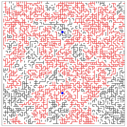
(a)

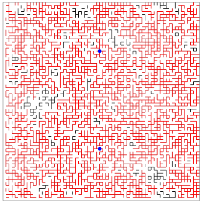
(b)

Figure 1: Two illustrations of the system are presented for a lattice of size $64\times 64$ with periodic boundary conditions, and with $k=2$ anchor points (marked by filled blue circles) separated by a distance of $32$ lattice units. Bonds of the largest occupied cluster are shown in red (grey), and all other occupied bonds are shown in black. (a) A system where the number of bonds is exactly 4096 or $p=4096/8192=1/2=p_{c}$, without connection between the two anchor points. (b) The same system where the number of occupied bonds is increased to 4415 bonds or $p_{c2}=4415/8192\approx 0.53894$, at which point connection between the anchors first occurred. This is a typical example where the threshold is near the average value of $\overline{p}_{c2}=0.5322$ and shows that in this supercritical regime there is a percolating network that goes essentially throughout the entire system.

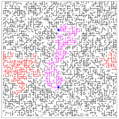
(a)

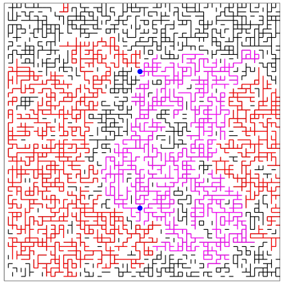
(b)

Figure 2: (a) Here the density of occupied bonds at the first connection occurs at $p=p_{c2}=3660/8192=0.44678$. (b) The same system where $p$ is increased to $p_{c}=1/2$ is shown. This is a very rare system in which the connection between the anchor points first occurs substantially below $p_{c}$, where the point connecting cluster (magenta or light grey bonds) is different from the largest cluster (red or grey bonds). In fact, the spanning cluster is relatively small and does not extend over the whole system. Such behavior where spanning occurs below $p_{c}$ can only happen in smaller systems. In most cases, the individual values of $p_{c2}$ are larger than $p_{c}$ and the cluster connecting them is the “infinite” cluster that spreads over virtually the entire system as in Fig. 1(b).

II.2 Scaling of the estimates

If we assume that the mapping of our problem to $[P_{\infty}(p)]^{k}$ is correct for finite systems characterized by $P_{\infty}(p,L)$, we can then estimate the scaling behavior of the estimates from finite-size scaling theory. That theory states that for $L\to\infty$ and $p-p_{c}\to 0$ with $(p-p_{c})L^{1/\nu}$ constant,

$$P_{\infty}(p,L)\sim aL^{-\beta/\nu}F(b(p-p_{c})L^{1/\nu})$$ (5)

where $a$ and $b$ are system-dependent constants (“metric factors”) while $\beta$, $\nu$ and $F(z)$ are universal quantities, having the same values and behavior for all systems of a given dimensionality, and also a given system shape for the case of $F(z)$. For $d=2$, one has $\beta=5/36$ and $\nu=4/3$ StaufferAharony94 .

We will apply this scaling to the estimate for $\overline{p}_{ck}$ given by Eq. (3). First we consider the interval $p=(0,p_{c})$. In this interval, we assume that the finite-size effects are essentially those given by the scaling function $F(z)$, because when $p<p_{c}$, $P_{\infty}(p,\infty)=0$. That is, we assume the non-scaling corrections are unimportant for large $L$ for $p<p_{c}$.

Putting (5) into the integral in Eq. (3) over the interval $p=(0,p_{c})$, we find

$$\int_{0}^{p_{c}}[P_{\infty}(p)]^{k}dp=a^{k}\int_{0}^{p_{c}}L^{-k\beta/\nu}[F(b(p-p_{c})L^{1/\nu})]^{k}dp$$ (6)

and a change of variables yields

$$\int_{0}^{p_{c}}[P_{\infty}(p)]^{k}dp = a^{k}b^{-1}L^{-(k\beta+1)/\nu}\int_{-bp_{c}L^{1/\nu}}^{0}[F(z)]^{k}dz$$ (7)

$$\approx a^{k}b^{-1}L^{-(k\beta+1)/\nu}\int_{-\infty}^{0}[F(z)]^{k}dz$$ (9)

where $z=b(p-p_{c})L^{1/\nu}$. In the second integral in (9) we extended the lower limit to $-\infty$, valid for large $L$ because the integrand decays exponentially for negative $z$.

Therefore, this contribution to the integral in (3) should scale as $L^{-1/\nu_{k}}$ with

$$1/\nu_{k}=(k\beta+1)/\nu=\frac{36+5k}{48}$$ (10)

so that $1/\nu_{1}=41/48=0.854166$ and $1/\nu_{2}=23/24=0.958333$ etc.

For $p>p_{c}$, it is not clear how to attack the finite-size corrections of the integral in (3) because there are large non-scaling contributions to $P_{\infty}$ whose behavior we do not know, but it seems reasonable to assume that the finite-size corrections for $p>p_{c}$ scale the same as those we found for $p<p_{c}$, so we conjecture that the exponents $\nu_{k}$ above should characterize the full finite-size corrections to $\overline{p}_{ck}$. That is, we conjecture

$$\overline{p}_{ck}(L)=\overline{p}_{ck}+cL^{-1/\nu_{k}}$$ (11)

where $c$ is a constant and $\nu_{k}$ is given by Eq. (10). The constant term on the right-hand side, $\overline{p}_{ck}$, derives from the non-scaling parts of $P_{\infty}$ for $p>p_{c}$.

Note that it also follows from the scaling arguments above that $P_{r}=k[P_{\infty}(p)]^{k-1}P^{\prime}_{\infty}(p)$ behaves with $L$ in the scaling regime as

$$P_{r} \sim ka^{k-1}L^{-(k-1)\beta/\nu}[F(b(p-p_{c})L^{1/\nu})]^{k-1}$$ (12)

$$\times aL^{-\beta/\nu}F^{\prime}(b(p-p_{c})L^{1/\nu})bL^{1/\nu}$$ (13)

$$\sim L^{-(k\beta-1)/\nu}G(b(p-p_{c})L^{1/\nu})$$ (14)

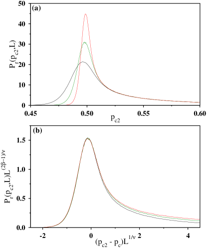
Figure 3: Simulation result: (a) The probability distribution $P_{r}(p_{c2},L)$ of the percolation threshold $p_{c2}$ of connecting two anchor points has been plotted against $p_{c2}$ for $L$ = 128 (black or lower curve), 256 (green or middle curve), 512 (red or upper, most peaked curve). (b) The scaling plot of the probability distribution $P_{r}(p_{c2},L)L^{(2\beta-1)/\nu}$ against $(p_{c2}-p_{c})L^{1/\nu}$ with $\beta=5/36,\nu=4/3$ with $p_{c}=1/2$. Bottom to top $L=128$, 256, and 512.

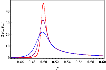
Figure 4: Plots of $P_{r}(p,L)=2P_{\infty}(p)P^{\prime}_{\infty}(p)$ for $L=128,$ 256 and 512, bottom to top at peaks. These are the analogous curves as given in Fig. 3(a), calculated from $P_{\infty}(p)$ rather than by direct simulation of $P_{r}$. Note here $p$ is equivalent to $p_{c2}$ used in Fig. 3.

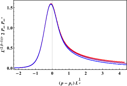
Figure 5: Scaling plot of $L^{(2\beta-1)/\nu}2P_{\infty}(p)P^{\prime}_{\infty}(p)$ vs. $(p-p_{c})L^{1/\nu}$ for $L=128,$ 256 and 512 (bottom to top). The curves collapse well to a universal curve, except for the tail for large $(p-p_{c})L^{1/\nu}$ which represents the non-scaling part of this quantity. This plot is comparable with Fig. 3(b), here evaluated through $P_{\infty}$ rather than the direct measurement of $P_{r}$. Here $p$ is equivalent to $p_{c2}$ in Fig. 3.

III Simulation methods

III.1 Simulation method to find $\overline{p}_{ck}$

We carried out computer simulations of these processes on systems of size $L\times L$ for bond percolation, with periodic boundary conditions. For the case $k=1$, we consider $L$ odd and add bonds until the center point connects to the boundary for $p=p_{c1}$. Repeating this process many times, we average the values of $p_{c1}$ to find $\overline{p}_{c1}$. For $k$ = 2, 3 and 4, we consider periodic $L\times L$ systems with $L=2^{n}$, $n=5,6,\ldots 12$. For $k=2$ we consider the connectivity between a point at the origin (0,0) and a point at $(0,L/2)$. For $k=3$, the connectivity between the three points (0,0), $(L/2,0)$, and $(0,L/2)$, and for $k=4$, the connectivity between the four points (0,0), $(L/2,0)$, $(0,L/2)$, and $(L/2,L/2)$ is considered. Note that for $k=3$, the three points are the vertices of a right triangle rather than an equilateral triangle, so the distances between pairs of points are not identical, but this is not important — all that matters is that the three points are relatively far apart from each other. The average value of $p$ at the first connection gives $\overline{p}_{ck}$.

It is clear from Eq. (1) that the values of the thresholds $\overline{p}_{ck}$ should depend only on the value of $k$, and not on the actual distribution of the $k$ points. We have numerically verified this issue for $k=2$ by randomly distributing these two points on the lattice for every configuration. Our simulation results show that the values of $\overline{p}_{c2}$ remain unchanged.

We also studied the average $p$ at which the origin connects to point $x=1$, $x=2$, …, $x=L/2$ and $y=0$ for systems of different $L$. We discovered that $p_{c2}(x)$ does not noticeably depend upon $L$ as along as $x\ll L$, indicating that the size of the system is unimportant for shorter-range connections.

III.2 Simulation method to find $P_{\infty}$

To test the conjecture relating $\overline{p}_{ck}$ to $P_{\infty}$, we carried out measurements of $P_{\infty}(p)$ using the method of Newman and Ziff (NZ) NewmanZiff00 ; NewmanZiff01 , which involves adding bonds one at a time to the system and using the union-find procedure to merge clusters and keep track of the cluster distribution. This method allows one to effectively measure a quantity $Q(p)$ (such as $P_{\infty}(p))$ for all values of $p$ in a single simulation. In this method, one first determines the “microcanonical” $Q_{n}$ (here $P_{\infty,n}$) when exactly $n$ bonds have been placed down, and then determines the “canonical” $Q(p)$ (here $P_{\infty}(p)$) by carrying out a convolution with the binomial distribution $B(N,n,p)={N\choose n}p^{n}(1-p)^{N-n}$:

$$Q(p)=\sum_{n=0}^{N}{N\choose n}p^{n}(1-p)^{N-n}Q_{n}$$ (15)

where $N$ is the total number of bonds in the system, in this case $2L^{2}$. For large systems, the differences between the microcanonical $Q_{n}$ with $n=pN$ and $Q(p)$ are small, except for regions of high curvature or second derivative, but the convolution serves a further purpose of smoothing out the data, and connecting it with a continuous curve, rather than the discrete values $p=1/N,2/N,\ldots$. To integrate $P_{\infty}(p)$ (as required for $\overline{p}_{c1}$ according Eqs. (3) or (4)), one can just as well sum the microcanonical values, because of the identity ZiffNewman02

$$\int_{0}^{1}Q(p)dp = \sum_{n=0}^{N}{N\choose n}Q_{n}\int_{0}^{1}p^{n}(1-p)^{N-n}dp$$ (16)

$$= \frac{1}{N+1}\sum_{n=0}^{N}Q_{n}$$ (17)

Likewise it follow that

$$\int_{0}^{1}pQ(p)dp = \frac{1}{(N+1)(N+2)}\sum_{n=0}^{N}(n+1)Q_{n}$$ (18)

To integrate $[Q(p)]^{k}=[P_{\infty}(p)]^{k}$ for $k>1$ with respect to $p$, it is most straightforward to first carry out the convolution to find $P_{\infty}(p)$, and then numerically integrate the $[P_{\infty}(p)]^{k}$ at equally spaced values of $p$.

Derivatives of $Q(p)$ can also be found directly from the $Q_{n}$ ZiffNewman02 :

$$Q^{\prime}(p) = \sum_{n=0}^{N}{N\choose n}Q_{n}\frac{d}{dp}\left(p^{n}(1-p)^{N-n}\right)$$ (19)

$$= \frac{1}{p(1-p)}\sum_{n=0}^{N}(n-Np){N\choose n}(p^{n}(1-p)^{N-n})Q_{n}$$ (20)

$$= \frac{\langle(n-Np)Q_{n}\rangle}{p(1-p)}$$ (21)

and likewise

$$\textstyle{Q^{\prime\prime}(p)} =\textstyle{\frac{\langle n^{2}Q_{n}\rangle-(2(N-1)p+1)\langle nQ_{n}\rangle+N(N-1)p^{2}\langle Q_{n}\rangle}{p^{2}(1-p)^{2}}\hskip 10.00002pt}$$ (22)

$$\textstyle{=} \textstyle{\frac{\langle(n-Np)^{2}Q_{n}\rangle+(2p-1)\langle(n-Np)Q_{n}\rangle-Np(1-p)\langle Q_{n}\rangle}{p^{2}(1-p)^{2}}}$$ (23)

where the averages are over the binomial distribution $B(N,n,p)$. Note that in Ref. ZiffNewman02 , there is a typo in Eq. (32) for $Q^{\prime\prime}(p)$, in which the last term should have the factor $(N-n-1)$ rather than $(N-n+1)$.

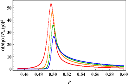
Figure 6: A plot of $(d/dp)[P_{\infty}(p)]^{k}$ vs. $p$ for $k=1$ (red, highest peak)), $k=2$ (orange, second-highest peak), $k=3$ (green, second-lowest peak), and $k=4$ (blue, lowest peak) for a system with $L=512$, calculated from the results of the numerical simulations of $P_{\infty}(p)$, including using Eq. (21) to find $P^{\prime}_{\infty}(p)$. The estimates of $\overline{p}_{ck}$ are the means of these distributions according to Eq. (2), and it can be seen that the distribution spreads to the right as $k$ increases, yielding larger values of $\overline{p}_{ck}$. To find the accurate values of $\overline{p}_{ck}$, one has to consider systems of different $L$ and take the limit that $L\to\infty$, although the change is small for systems larger than $L=512$. Note that the distribution is broad and the large fluctuations in the individual values of $p_{ck}$ persist as $L\to\infty$.

To find $P_{\infty}(p)$ we simulated $10^{7}$ samples each for $L=64,128,256$ and 512 on $L\times L$ periodic systems, saving the $2L^{2}$ microcanonical values of $s_{\mathrm{max}}$ in a file. For the largest system $L=512$, the simulations took several days on a laptop computer. Then we used a separate program to read the files and calculate $P_{\infty}(p)=s_{\mathrm{max}}/L^{2}$ for $10^{4}$ points $p=0,0.0001,\ldots,1.0000$ using the convolution (15). We also calculated $P^{\prime}_{\infty}(p)$ and $P^{\prime\prime}_{\infty}(p)$ using the formulas of Eqs. (21) and (23). We used the recursive method described in Ref. NewmanZiff01 to calculate the binomial distribution for each $p$. To find the integrals of $[P_{\infty}(p)]^{k}$ for Eqs. (3) and (4), we carried out numerical integration of the $10^{4}$ points using the trapezoidal rule (namely counting the two endpoints with relative weight 1/2 and all other points with weight 1). We compared some of the integrals using $10^{3}$ and $10^{5}$ points and did not find significant difference in the results, and used $10^{4}$ values of $p$ in our calculations.

IV Results

Figure 3(a) shows the probability distribution $P_{r}(p_{c2},L)$ of the percolation threshold $p_{c2}$ of connecting two anchor points, from direct measurements. Note $p_{c2}$ is the value of $p$ at which the connection first takes place in a given sample, as opposed to $\overline{p}_{c2}$ which is the average value over many samples. Figure 3(b) shows a scaling plot of the data, using the scaling implied in Eq. 14.

Figure 4 shows the predicted behavior of $P_{r}$ from the ansatz of Eq. 1, using the simulation results of $P_{\infty}$ rather than measuring $P_{r}$ directly. These curves can be compared with those of Fig.  3(a), and the two can be seen to agree.

Figure 5 shows the predicted scaling behavior of $P_{r}$ from the ansatz of Eq. 1, and the results can be seen to be similar to the scaling plot of the directly measured $P_{r}$ given in Fig. 3(b).

Figure 6 shows plots of the predicted distributions of the probabilities of first connection, $(d/dp)[P_{\infty}(p)]^{k}$, for $k=1$, 2, 3, and 4, based upon measurements $P_{\infty}(p)$, for a system of $L=512$. As can be seen, the distributions are broad, meaning that the thresholds we find $p_{ck}$ have large fluctuations from system to system and persist as $L\to\infty$.

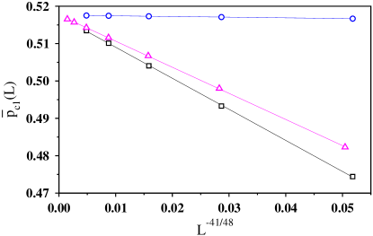
Figure 7: Values of $\overline{p}_{c1}(L)$ found from simulations of connections of a point at the center to the boundary of an $(L+1)\times(L+1)$ square system (triangles), by integrating $P_{\infty}(p)$ on $L\times L$ periodic systems using Eq.  (3) for $k=1$ (squares), and by integrating $P_{\infty}(p)$ using Eq.  (4) (circles). The estimates are all plotted vs.  $L^{-41/48}$ according to the prediction of Eq.  (10). The equations of the linear fits through the points are $\overline{p}_{c1}=a+bL^{-41/48}$ with $a=0.55520$, $b=-0.33805$ (squares), $a=0.55532$, $b=-0.27962$ (triangles), $a=0.55530$, $b=-0.06323$ (circles).

In Fig. 7 we plot estimates for $\overline{p}_{c1}$ found from direct simulations with the point in the center of an $(L+1)\times(L+1)$ system, for $L=64,128,\ldots,4096$, and secondly using the formulas of Eqs.  (3) and (4) for $k=1$ based upon $P_{\infty}(p)$. The data are plotted based on the predicted scaling $L^{-41/48}$ from Eq. (10). We do not expect that the values of $\overline{p}_{c1}(L)$ would be the same for finite $L$ from the two methods (direct simulation and via $P_{\infty}$); however, we expect that the extrapolation as $L\to\infty$ should be the same, because in that limit the probability the point connects to the boundary should exactly be the probability the point belongs to the largest cluster, namely $P_{\infty}$. Furthermore, we expect the two estimates of $\overline{p}_{c1}$ should scale with $L$ with the same exponent $1/\nu_{1}=41/48$, and indeed that plot confirms that expectation. The two different approaches suggest a threshold of $\overline{p}_{c1}=0.51749(5)$.

It can clearly be seen that the estimate based upon (4), which assumes $P_{\infty}(p,L)=0$ for $p<p_{c}$, converges much more quickly than the estimate based upon (3). On a more expanded scale, the convergence to this estimate is also shown to obey the $L^{-41/48}$ scaling, but is not shown here. The results for $k=2$, 3 and 4 are shown in Figs. 8, 9, and 10. Our values of $p_{ck}$ are given in Table 1.

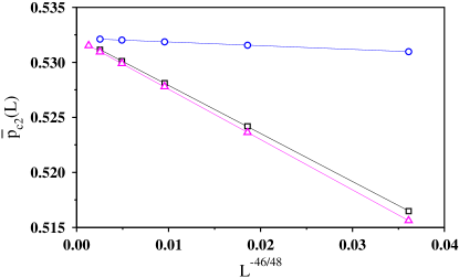
Figure 8: Values of $\overline{p}_{c2}(L)$ found from direct simulations on an $L\times L$ periodic system with the two points at (0,0) and (0,$L/2$) (triangles), and the predictions from Eqs. (3) (squares) and (4) (circles) based upon measurements of $P_{\infty}(p)$ on an $L\times L$ periodic system, all plotted as a function of $L^{-46/48}=L^{-23/24}$ as predicted by Eq. (10). Here $L=32$, 64, 128, 256, and 512 for the upper two sets of data, and also $L=1024$ for the lower set.

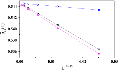
Figure 9: Values of $\overline{p}_{c3}(L)$ found from direct simulations on an $L\times L$ periodic system with the three points at (0,0), $(0,L/2)$ and ($L/2,0$) (triangles), and the predictions from Eqs. (3) (squares) and (4) (circles) based upon measurements of $P_{\infty}(p)$ on an $L\times L$ periodic system, all plotted as a function of $L^{-51/48}=L^{-17/16}$ as predicted by Eq. (10).

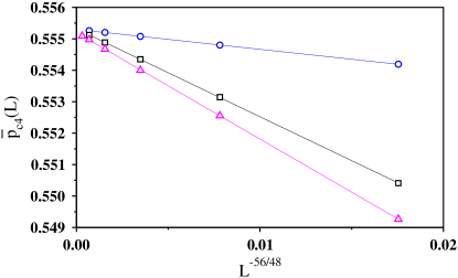
Figure 10: Values of $\overline{p}_{c4}(L)$ found from direct simulations on an $L\times L$ periodic system with the four points at the corners of a square of length $L/2$ (triangles), and the predictions based upon $P_{\infty}(p)$ using Eq. (3) (squares) and Eq. (4) (circles), both based upon measurements of $P_{\infty}(p)$ on an $L\times L$ periodic system. All data are plotted as a function of $L^{-56/48}=L^{-7/6}$ as predicted by Eq. (10). Lines show linear fits through the data. It can be seen that estimates based upon Eq. (4) exhibit the fastest convergence with system size.

V Correlations

We also considered a related question for two- and three-point correlations. Studying this problem sheds light on the correlations that occur in the system in the critical vs. the post-critical regime where the connectivity between the anchor points mainly occurs.

In SimmonsZiffKleban09 ; DelfinoViti10 the following ratio was considered:

$$R(p)=\frac{P(r_{1},r_{2},r_{3})}{\sqrt{P(r_{1},r_{2})P(r_{1},r_{3})P(r_{2},r_{3})}}$$ (24)

where $r_{1}$, $r_{2}$ and $r_{3}$ are three points in the system, $P(r_{i},r_{j})$ is the probability that points $r_{i}$ and $r_{j}$ connect, and $P(r_{1},r_{2},r_{3})$ is the probability that all three points connect.

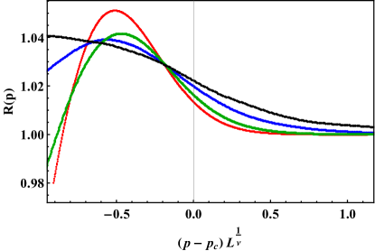
Figure 11: (color online) Scaling plot of $R(p)$ vs. $(p-p_{c})L^{1/\nu}$ where $R(p)$ is given in Eq. (24), for three points at positions ($0,0$), ($0,L/n$), and ($L/n,0$), for $n=2$ (red, the curve with the highest peak), $n=4$, (green, the curve with the second-highest peak), $n=8$ (blue, the curve with the third-highest peak), and $n=16$ (black, the curve that does not reach a peak in this interval), for $L=64$, 128, 256, and 512 respectively. Other runs show that there is a small $L$-dependence on the results, but the main variation is due to $n$. At $p=p_{c}=1/2$, the value of $R(p_{c})$ approaches the theoretical value $C_{1}=1.022$ SimmonsZiffKleban09 ; DelfinoViti10 as $n$ gets large, in which case the three points are close together compared to the size of the system. The meaning of the crossing point for $(p-p_{c})L^{1/\nu}\approx-0.2$ is unclear, and may not be maintained for larger systems.

This ratio has previously been studied, to our knowledge, only at $p=p_{c}$, where the value of $R(p_{c})$ approaches the value $C_{1}=1.0220$ when the three points are far separated and the system size is infinite. This value of $C_{1}$ was first observed numerically in SimmonsZiffKleban09 and then derived analytically from conformal field theory in DelfinoViti10 . The fact that this ratio is unequal to 1 implies a correlation between the three points in the system. If we make the assumption that $P(r_{i},r_{j})=P_{\infty}(p)^{2}$ and $P(r_{1},r_{2},r_{3})=P_{\infty}(p)^{3}$, which we expect to be the case for $p>p_{c}$, then we would have $R=1$. At $p_{c}$, where the infinite cluster does not span throughout the system, one would not expect this to be valid and indeed $R(p)\neq 1$, although it turns out quite close to 1.

Here we consider the three points in a right triangle, ($0,0$), ($0,L/n$), and ($L/n,0$), in an $L\times L$ periodic system, for $n=2,$ 4 and 8 . As $n$ increases for large $L$ (that is, as the separation of the three points is small compared to the size of the system), $R(p_{c})$ approaches the value $C_{1}$. Using the NZ method, we were able to calculate $R(p)$ as a function of $p$ after executing a microcanonical simulation where we found the $P(r_{i},r_{j})$ and $P(r_{1},r_{2},r_{3})$ as a function of the number of bonds added. We then carried out the convolution to the canonical ($p$-dependent) functions for all $P$’s separately, and calculated $R(p)$ according to Eq. (24). The results are shown in Fig. 11.

As can be seen, at $p=p_{c}$, $R(p_{c})$ approaches $C_{1}$ as $n$ increases (in which case the points get closer together compared to the size of the system). In the limit that $L\to\infty$, $R(p)$ evidently becomes a discontinuous function of $p$, with $R(p_{c})=C_{1}$ for $p=p_{c}$, and $R(p)=1$ for $p>p_{c}$. The behavior for $p<p_{c}$ is not clear. Notice in Fig. 11 that there is a maximum for $R(p)$ in finite systems at $z=(p-p_{c})L^{1/\nu}\approx-0.5$, meaning for some values of $p<p_{c}$, $R(p)$ is greater than the value at $p_{c}$. However, it is not clear what the behavior is as $n\to\infty$ (for large $L$); it is possible that the peak for negative $z$ disappears and the peak occurs only at $z=0$ or $p=p_{c}$. The behavior for $p<p_{c}$ needs further investigation.

At the point $p_{c3}\approx 0.5445$ where three points first connect, it can be seen that $R(p)$ approaches 1, since that would correspond to $(p-p_{c})L^{1/\nu}$ going to infinity as $L$ goes to infinity. This result reiterates that at the places where multiple points connect, there are no correlations among connections between different pairs of widely separated points.

Table 1: Our best estimates for the extrapolated values of the average percolation thresholds $\overline{p}_{ck}$ from direct measurements (second column) and from $P_{\infty}$ via Eqs. (3) and (4) for different values of $k$. The averages of these values are quoted in the abstract.

$k$	$\overline{p}_{ck}$ measured	Eq. (3)	Eq. (4)
1	0.51749(5)	0.51761(3)	0.51755(3)
2	0.53212(5)	0.53220(3)	0.53226(3)
3	0.54450(5)	0.54458(3)	0.54461(3)
4	0.55520(5)	0.55530(3)	0.55531(3)

VI Discussion

We have shown that exploring the average value of the probability $p$ of bond occupation at which a certain number of separated points first connect leads to a new set of average thresholds. The distribution of the values of $p$ is broad, so that this threshold is not sharp as in the usual case of thresholds in percolation. For example, the median rather than the mean of the distribution would give a different value. We have shown that the values can be related to $P_{\infty}(p)$, and confirm this relation by simulation. From this theory it is apparent that while the percolation thresholds $\overline{p}_{ck}$ indeed depend on the number $k$ of points, their values are robust with respect to the actual spatial distribution of the $k$ points. For example, the $k$ points may either be symmetrically placed on the lattice or, they can be randomly distributed (for $L\to\infty$).

This work suggests further research in a variety of areas. It might be interesting to study these thresholds in higher dimensions, where the relations to $P_{\infty}(p)$ in Eqs. (3) and (4), and the scaling in (10) (but with $\nu$ and $\beta$ being the three-dimensional result) should still hold, for connections to points as we considered here. Furthermore, connections between higher-dimensional objects (lines, surfaces, …) can also be considered. One question to consider is whether the thresholds continue to have broad distributions as found here, and how those thresholds scale with $L$.

With respect to the correlations $R(p)$, one can consider a point in the center of a surface of a cylinder (that is, the center of a square with periodic b.c. in one direction), and find the probability of connecting the center to one boundary or to both boundaries of the cylinder. At $p_{c}$, the corresponding $R(p)$ should go to the value $C_{0}=2^{7/2}3^{-3/4}\pi^{5/2}\Gamma(1/3)^{-9/2}=1.0299268\ldots$ SimmonsZiffKleban09 while the behavior away from $p_{c}$ has not been studied before. Likewise, similar correlations in higher dimensions have not been studied. Many aspects of correlations in percolation are yet to be explored.

VII Acknowledgment

The authors would like to thank Deepak Dhar for a careful reading and constructive comments on the paper.

References

- [1] Dietrich Stauffer and Ammon Aharony. Introduction to Percolation Theory, 2nd ed. CRC press, 1994.
- [2] Peter J. Reynolds, H. Eugene Stanley, and W. Klein. Large-cell Monte Carlo renormalization group for percolation. Phys. Rev. B, 21:1223–1245, 1980.
- [3] L. S. Ramirez, P. M. Centres, and A. J. Ramirez-Pastor. Standard and inverse bond percolation of straight rigid rods on square lattices. Phys. Rev. E, 97:042113, 2018.
- [4] Wenxiang Xu, Zhigang Zhu, Yaqing Jiang, and Yang Jiao. Continuum percolation of congruent overlapping polyhedral particles: Finite-size-scaling analysis and renormalization-group method. Phys. Rev. E, 99:032107, 2019.
- [5] Sumanta Kundu and S. S. Manna. Percolation model with an additional source of disorder. Phys. Rev. E, 93:062133, 2016.
- [6] Sayantan Mitra, Dipa Saha, and Ankur Sensharma. Percolation in a distorted square lattice. Phys. Rev. E, 99:012117, 2019.
- [7] M. G. Slutskii, L. Yu. Barash, and Yu. Yu. Tarasevich. Percolation and jamming of random sequential adsorption samples of large linear -mers on a square lattice. Phys. Rev. E, 98:062130, 2018.
- [8] Shogo Mizutaka and Takehisa Hasegawa. Disassortativity of percolating clusters in random networks. Phys. Rev. E, 98:062314, 2018.
- [9] Sumanta Kundu, Nuno A. M. Araújo, and S. S. Manna. Jamming and percolation properties of random sequential adsorption with relaxation. Phys. Rev. E, 98:062118, 2018.
- [10] Yunqing Ouyang, Youjin Deng, and Henk W. J. Blöte. Equivalent-neighbor percolation models in two dimensions: Crossover between mean-field and short-range behavior. Phys. Rev. E, 98:062101, 2018.
- [11] Wei Huang, Pengcheng Hou, Junfeng Wang, Robert M. Ziff, and Youjin Deng. Critical percolation clusters in seven dimensions and on a complete graph. Phys. Rev. E, 97:022107, 2018.
- [12] Stephan Mertens and Cristopher Moore. Percolation thresholds and fisher exponents in hypercubic lattices. Phys. Rev. E, 98:022120, 2018.
- [13] Stephan Mertens and Cristopher Moore. Series expansion of the percolation threshold on hypercubic lattices. J. Phys. A: Math. Th., 51(47):475001, 2018.
- [14] Cesar I. N. Sampaio Filho, José S. Andrade, Hans J. Herrmann, and André A. Moreira. Elastic backbone defines a new transition in the percolation model. Phys. Rev. Lett., 120:175701, 2018.
- [15] M. M. H. Sabbir and M. K. Hassan. Product-sum universality and rushbrooke inequality in explosive percolation. Phys. Rev. E, 97:050102(R), 2018.
- [16] S. M. Flores, J. J. H. Simmons, P. Kleban, and R. M. Ziff. A formula for crossing probabilities of critical systems inside polygons. J. Phys. A: Math. Th., 50(6):064005, 2017.
- [17] John C. Wierman. On bond percolation threshold bounds for archimedean lattices with degree three. J. Phys. A: Math. Th., 50(29):295001, 2017.
- [18] Robert M. Ziff and Salvatore Torquato. Percolation of disordered jammed sphere packings. J. Phys. A: Math. Th., 50(8):085001, 2017.
- [19] Ivan Kryven, Robert M. Ziff, and Ginestra Bianconi. Renormalization group for link percolation on planar hyperbolic manifolds. Phys. Rev. E, 100:022306, 2019.
- [20] Jacob J. H. Simmons, Robert M. Ziff, and Peter Kleban. Factorization of percolation density correlation functions for clusters touching the sides of a rectangle. J. Stat. Mech. Th. Exp., 2009(02):P02067, 2009.
- [21] Gesualdo Delfino and Jacopo Viti. On three-point connectivity in two-dimensional percolation. J. Phys. A.: Math. Th., 44(3):032001, 2010.
- [22] M. E. J. Newman and R. M. Ziff. Efficient Monte Carlo algorithm and high-precision results for percolation. Phys. Rev. Lett., 85(19):4104–4107, 2000.
- [23] M. E. J. Newman and R. M. Ziff. Fast Monte Carlo algorithm for site or bond percolation. Phys. Rev. E, 64(1):016706, 2001.
- [24] R. M. Ziff and M. E. J. Newman. Convergence of threshold estimates for two-dimensional percolation. Phys. Rev. E, 66(1):016129, 2002.