Lasing in a coupled hybrid double quantum dot-resonator system

Abstract

We theoretically investigate the possibility of lasing in an electromagnetic resonator coupled to a voltage-biased hybrid-double-quantum-dot comprised of a double-quantum-dot tunnel coupled simultaneously to a normal metal and a superconducting lead. Using a unitary transformation, we derive a resonator-double-quantum-dot interaction Hamiltonian in the rotating wave approximation which reveals the fact that lasing in this system is mediated by electron transitions between Andreev energy levels in the system’s density of states. Moreover, by employing a markovian master equation incorporating dissipation effects for the electronic and photonic degrees of freedom, we numerically calculate the steady-state reduced density-matrix of the system from which we determine the average photon number and its statistics in the resonator in various parameter regimes. We find that at some appropriate parameter configurations, lasing can be considerably enhanced due to the possiblity of electron tansitions between multiple Andreev levels in the system.

I Introduction

Laser has been one of the most intriguing optical devices over the past few decades, and today it has found tremendous number of applications in different fields of the science and technology. While in conventional lasers, light amplification is induced by optical pumping of large number of atoms which are weakly coupled to the cavity mode, the realization of strongly coupled one-atom-laser in tightly confined cavity modes is of fundamental interest to the researchers due to their particular properties and usages(Mu and Savage, 1992; Ginzel et al., 1993; Pellizzari and Ritsch, 1994a, b; An et al., 1994; Jones et al., 1999; Löffler et al., 1997; Karlovich and Kilin, 2001). Following the first experimental achievement in 2003 using a single Cesium atom strongly coupled to a cavity mode(McKeever et al., 2003), many theoretical proposals and experimental demonstrations were put forward to explore other realizations of the single atom laser(Yoshie et al., 2004; Florescu et al., 2004; Aoki et al., 2006; Lougovski et al., 2007; Florescu, 2008; Kim et al., 2008; Ritter et al., 2010). Among of these, quantum dot(QD) lasers find a lot of interest because of their tunability as well as their fabrication advantages. In the last two decades, based on the cavity quantum electrodynamics, many micro and nano-cavity lasers with a single-QD have been fabricated(Reithmaier et al., 2004; Reitzenstein et al., 2008; Nomura et al., 2009, 2010; Ledentsov, 2010; Liu et al., 2011).

Recently, similar effects are demonstrated in the circuit quantum electrodynamics architecture, where a double-quantum-dot(DQD) or a superconducting qubit, which is constantly driven into an excited state by an external electric or magnetic bias, plays the role of an active media in the electromagnetic resonator formed in a superconducting transmission line(Marthaler et al., 2011; Jin et al., 2011; Toida et al., 2013; Liu et al., 2015; Karlewski et al., 2016; Stehlik et al., 2016; Astafiev et al., 2007; Hauss et al., 2008; Grajcar et al., 2008; André et al., 2009). In particular, it was theoretically predicted in Ref.[Jin et al., 2011] and then experimentally shown in Ref.[Liu et al., 2015], that a voltage biased DQD can create a lasing state when it is coupled to a resonator through an electric dipole interaction. By noting that, it was a DQD coupled to two normal metal leads which is actually considered in the aforementioned proposals to establish the lasing state in the resonator, it would be valuable to see whether replacing one of the normal metal leads by a superconductor can have any implications on the lasing behavior or not?

In general, by coupling a QD to a normal and also to a superconducting lead, some new intriguing features arise in the energy configurations and transport properties of the QD, which are basically due to the formation of the resonant Andreev reflections at the QD-superconducting lead interface(Sun et al., 1999a, b, 2001; Cuevas et al., 2001; Nurbawono et al., 2010; Barański and Domański, 2013; Weymann and Wójcik, 2015). Recently, the role of such hybrid single QD structures in creating a lasing state in an electromagnetic resonator becomes attractive(Bruhat et al., 2016; Rastelli and Governale, 2019), however, the consequences of using a hybrid-DQD in a voltage biased DQD laser has not been studied, so far. It should be noted that, Bruhat et.al.(Bruhat et al., 2018), have recently conducted an experiment on a hybrid-DQD system coupled to an electromagnetic resonator. They have not studied the lasing state in their setup, but instead, they investigated the mechanism of resonator-DQD coupling and observed a symmetric coupling between the hybrid-DQD and the resonator which is attributed directly to the roles of superconducting proximity effects in the DQD.

In this paper, we consider a setup comprising a hybrid-DQD which is capacitively coupled to an electromagnetic resonator. Using an analytical treatment of the Hamiltonian of the system and also a numerical simulation of the full quantum system in the steady state, we analyze the lasing state in various parameter regimes of this model system. We show that a lasing state with sub-Poissonian statistics is present in this system at frequencies equal to the energy differences between Andreev energy levels in the density of states of the hybrid DQD. There are two Andreev energy levels corresponding to each energy level of the hybrid DQD which are arranged in the density of states(DOS) of the system symmetrically around the chemical potential of the superconducting electrode. Therefore, depending on the weights of different Andreev levels in the DOS, there are some specific parameter regimes at which the system shows lasing due to the electron transitions between the corresponding Andreev energy levels of hybrid DQD.

The remainder of this paper is organized as follows: In Sec.II, the model Hamiltonian is introduced and the underlying formalism of the paper is set up. Our numerical results are considered in Sec.III, and conclusions are presented in Sec.IV.

II MODEL AND FORMALISM

II.1 Model Hamiltonian

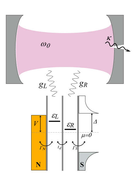
Figure 1: A single mode resonator is capacitively coupled to a voltage-biased hybrid double quantum dot connected to a normal metal and a superconducting lead.

As it is shown in Fig.1, our model system consists of a hybrid DQD, which is capacitively coupled to a single mode electromagnetic resonator. The total Hamiltonian of the system can be written as:

$$\hat{H}=\hat{H}_{dqd}+\hat{H}_{l}+\hat{H}_{l-d}+\hat{H}_{ph}+\hat{H}_{ph-dqd},$$ (1)

where $\hat{H}_{dqd}$ is the Hamiltonian of the DQD given by

$$\hat{H}_{dqd}= \sum_{\sigma}\varepsilon_{L}\hat{n}_{L,\sigma}+\varepsilon_{R}\hat{n}_{R,\sigma}+t_{d}\sum_{\sigma}(d_{R,\sigma}^{\dagger}d_{L,\sigma}+h.c)$$

$$+U_{R}\hat{n}_{R,\uparrow}\hat{n}_{R,\downarrow}+U_{L}\hat{n}_{L,\uparrow}\hat{n}_{L,\downarrow}+U_{LR}\hat{n}_{L}\hat{n}_{R},$$ (2)

where $\hat{n}_{i,\sigma}=\hat{d}_{i,\sigma}^{\dagger}\hat{d}_{i,\sigma}$ is the electron number operator with spin $\sigma=\uparrow,\downarrow$ in the dot $i=L,R$ with energy $\varepsilon_{i}$, and $t_{d}$ is the hybridization energy between DQDs. Moreover, $U_{L}$ and $U_{R}$ are the onsite Coulomb interaction energies for the left and right dots, respectively, and $U_{LR}$ is the mutual Coulomb interaction between the two dots in DQD. Furthermore, $\hat{H}_{l}$ and $\hat{H}_{l-d}$ stand for the Hamiltonian of the leads and tunneling between leads-DQD which are given by

$$\hat{H}_{l} =\underset{k,\alpha,\sigma}{\sum}(\varepsilon_{k,\alpha}+\mu_{\alpha})\hat{c}_{k,\alpha,\sigma}^{\dagger}\hat{c}_{k,\alpha,\sigma}$$

$$\qquad+\underset{k,\alpha}{\sum}\Delta_{\alpha}(\hat{c}_{k,\alpha,\uparrow}^{\dagger}\hat{c}_{k,\alpha,\downarrow}^{\dagger}+h.c),$$ (3)

$$\hat{H}_{l-d} =\sum_{k,\alpha,i,\sigma}t_{\alpha,i}(\hat{c}_{k,\alpha,\sigma}^{\dagger}\hat{d}_{i,\sigma}+h.c.),$$ (4)

where $\hat{c}_{\sigma}$ denotes annihilation operator for an electron with spin $\sigma$ in the single-particle state of the left ($\alpha=N$) or right lead ($\alpha=S$), characterized by the momentum $k$ with energy $\varepsilon_{k,\alpha}$, and $\mu_{\alpha}$ is the chemical potential of the corresponding lead. Moreover, $\Delta_{i}$ is the pairing energy gap in the respective lead which is given by $\Delta_{N}=0$ for the normal lead and a real positive $\Delta_{S}$ for the superconducting lead. Furthermore, $t_{\alpha,i}$ is the tunneling energy between lead $\alpha$ and dot $i$. The left(right) lead is only coupled to the left(right) dot, thus $t_{N,R}=t_{S,L}=0$.

Because we are interested in studying the impacts of the presence of superconducting pairing correlations on the lasing behavior in the DQD-resonator coupled system, it is reasonable to consider electronic transitions in the superconducting subgap regime and disregard the quasiparticle excitations in the continuum region of the superconducting lead. In practice, this is equal to consider a large superconducting gap limit, $\Delta_{S}\rightarrow\infty$, in which all energy scales of the system are smaller than the edges of the superconducting gap. By using a Green’s functions description(Trocha and Barnaś, 2014) or a Schrieffer-Wolf transformation(Nigg et al., 2015), it can be shown that in this so-called infinite-gap approximation, the superconductor lead is decoupled from right dot, leaving an effective pairing potential $\Gamma_{S}(\hat{d}_{R,\uparrow}^{\dagger}\hat{d}_{R,\downarrow}^{\dagger}+h.c)$ in the Hamiltonian of DQD, where $\Gamma_{S}=2\pi|t_{S,R}|^{2}\rho_{0}^{S}$ is the electron tunneling rate between DQD and superconducting lead in the wide-band approximation and $\rho_{0}^{S}$ is the lead’s density of states in its normal state. Thus, we can rewrite the Hamiltonian of the DQD as

$$\hat{H}_{dqd}^{SC}=\hat{H}_{dqd}+\Gamma_{S}(\hat{d}_{R,\uparrow}^{\dagger}\hat{d}_{R,\downarrow}^{\dagger}+h.c).$$ (5)

The Hamiltonian of the single mode resonator is given by $\hat{H}_{ph}=\hbar\omega_{0}(\hat{a}^{\dagger}\hat{a}+\frac{1}{2}),$ where $\hat{a}$ is the bosonic annihilation operator of the resonator mode with frequency $\omega_{0}$. The coupling of the DQD to the resonator is modeled by a capacitive interaction between electrons in the DQD and the electric field in the resonator and its Hamiltonian is given by

$$\hat{H}_{ph-dqd}=-\sum_{i,\sigma}g_{i}\hat{n}_{i,\sigma}(\hat{a}+\hat{a}^{\dagger}),$$ (6)

where $g_{i}$ is the coupling strength between the dot $i$ and the resonator mode.

II.2 Master equation description

The coupled DQD-resonator system can be driven into a non-equilibrium state by applying a finite bias voltage $\mu_{N}=eV_{b}$ on the normal electrode where $e$ is the charge of electron. Following the standard recipe for deriving the master equation, we consider the DQD-resonator subsystem with the Hamiltonian $\hat{H}_{S}=\hat{H}_{dqd}^{SC}+\hat{H}_{ph}+\hat{H}_{ph-dqd}$, as an open system which we seek for its dynamics when it is weakly coupled to the normal metal electrode and a photon bath. Then, the dynamics of the system can be described by using a master equation of the reduced density matrix, $\rho$, of the coupled DQD-resonator system which in the Markovian approximation is given by(Gullans et al., 2018; Agarwalla et al., 2019)

$$\frac{d}{dt}\hat{\rho}(t)=- \frac{i}{\hbar}\big{[}\hat{H}_{S},\hat{\rho}(t)\big{]}+\mathcal{L}_{ph}\hat{\rho}(t)+\mathcal{L}_{N}\hat{\rho}(t),$$ (7)

where $\mathcal{L}_{ph}$ and $\mathcal{L}_{N}$ are, repectively, the Lindblad superoperators describing the dissipation of photons, and the electron tunneling between the QD and the normal metal electrode. While for a general description of the dynamics of the DQD-resonator system, a precise microscopic derivation of the above Lindblad superoperators is necessary, but as we are interested here to investigate the possibility of lasing in the hybrid DQD-resonator system, we will focus on the situations where the system is in low-temperatures and also there is a large bias voltage applied on the normal metal lead. These assumptions introduce great simplifications in our calculations and allow us to represent the action of the above Lindblad superoperators on the reduced density matrix of DQD-resonator by the following forms:

$$\mathcal{L}_{ph}\hat{\rho}(t)=\kappa\big{[}\hat{a}\hat{\rho}(t)\hat{a}^{\dagger}-\frac{1}{2}\big{\{}\hat{a}^{\dagger}\hat{a},\hat{\rho}(t)\big{\}}\big{]},$$ (8)

and

$$\mathcal{L}_{N}\hat{\rho}(t)=\Gamma_{N}\sum_{i,\sigma}\big{[}\hat{C}_{i\sigma}\hat{\rho}(t)\hat{C}_{i\sigma}^{\dagger}-\frac{1}{2}\big{\{}\hat{C}_{i\sigma}^{\dagger}\hat{C}_{i\sigma},\hat{\rho}(t)\big{\}}\big{]},$$ (9)

where $\kappa$ is the decay rate of the photons in the resonator, $\Gamma_{N}=2\pi|t_{N,L}|^{2}\rho_{0}^{N}$ is the electronic tunneling rate to the normal metal lead, and $\hat{C}_{i\sigma}=\hat{d}_{i,\sigma}^{\dagger}(\hat{d}_{i,\sigma})$, for positive(negative) bias voltages. We emphasize that if we had not considered the infinite-gap approximation for the superconducting lead, it would have been necessary in Eq.(7) to consider the effect of coupling to the superconducting lead by introducing its corresponding Lindblad superoperator(Pfaller et al., 2013). We also note that the above formalism best describes the coupled DQD-resonator system when the coupling between DQD and resonator is weak. For a general treatment in the presence of strong coupling between the DQD and the resonator we can refer to the Ref.[Agarwalla et al., 2019].

By solving Eq.(7) for $d\hat{\rho}(t)/dt=0$, we obtain the reduced density matrix of the coupled DQD-resonator system in the steady state, from which we can calculate the average value of every observable of the system using the relation $\bigl{\langle}\hat{O}(t)\bigr{\rangle}=\text{Tr}\bigl{[}\hat{O}\hat{\rho}(t)\bigr{]}$, where $\text{Tr}[...]$ is the trace with respect to all degrees of freedom in the system. Of interest to us here are the average photon number, $n_{photon}=\bigl{\langle}a^{\dagger}a\bigr{\rangle}$, and the Fano factor of the photons where the latter can be calculated by the relation $F=(\bigl{\langle}a^{\dagger}aa^{\dagger}a\bigr{\rangle}-\bigl{\langle}a^{\dagger}a\bigr{\rangle}^{2})/\bigl{\langle}a^{\dagger}a\bigr{\rangle}$. The Fano factor can be referred to as a means to distinguish between the photon bunching($F>1$) or anti-bunching($F<1$) regimes and describes whether the photons inside the resonator have either sub-Poissonian($F<1$), Poissonian($F=1$) or super-Poissonian($F>1$) statistics.(Mendes and Mora, 2016)

With the knowledge of the reduced density matrix of the system, we can also calculate the distribution of the photons number in the resonator, which is given by the diagonal elements of $\text{Tr}_{QD}\bigl{[}\hat{\rho}(t)\bigr{]}$ in the occupation number basis, where $\text{Tr}_{QD}[...]$ is the trace with respect to the degrees of freedom of the QD.

II.3 Rotating-wave-approximation

Despite its simplicity, Eq.(7) cannot be solved analytically and it is necessary to solve it numerically. Before presenting our numerical results, it is instructive to examine the Hamiltonian of the system in a rather different representation which is more familiar in the context of the quantum optics literature(Breuer et al., 2002). By transforming to a representation in which the Hamiltonians $\hat{H}_{dqd}^{SC}$ and $\hat{H}_{ph}$ are diagonal, we can find a rotating-wave-approximation(RWA) description of $\hat{H}_{ph-dqd}$ by which a clear interpretation of the lasing mechanism can be obtained easily. However, the simultaneous presence of pairing($\Gamma_{S})$ and tunneling($t_{d}$) terms in $\hat{H}_{dqd}^{SC}$, makes its analytical diagonalization practically impossible. Nevertheless, we can use perturbation theory to obtain a unitary transformation to the lowest order in $\Gamma_{S}$, which can be used to obtain an approximating expression for diagonalized $\hat{H}_{dqd}^{SC}$.

We relegate the details of deriving such unitary transformation to the AppendixA, and here we solely present the results. Using a unitary transformation $\hat{U}$, which its explicit representation is given in Eq.(17), the Hamiltonian $\hat{H}_{dqd}^{SC}$ becomes diagonalized as

$$\hat{\widetilde{H}}_{dqd}^{SC}=\hat{U}^{\dagger}\hat{H}_{dqd}^{SC}\hat{U}=\sum_{i,\sigma}E_{i}\hat{\gamma}_{i,\sigma}^{\dagger}\hat{\gamma}_{i,\sigma}+\mathcal{O}(\Gamma_{S}^{2}),$$ (10)

where $E_{1}(E_{2})=(\varepsilon_{L}+\varepsilon_{R})/2\pm[((\varepsilon_{L}-\varepsilon_{R})/2)^{2}+t_{d}^{2}]^{1/2}$ and the fermionic operators $\hat{\gamma}_{i,\sigma}$ with $i=1,2$ and $\sigma=\uparrow,\downarrow$, are related to the $\hat{d}_{i,\sigma}$ operators through Eq.(17). By applying the same unitary transformation on the DQD-resonator coupling Hamiltonian, $\hat{H}_{ph-dqd}$, and after some algebra, we reach to the following expression for the transformed Hamiltonian $\hat{\widetilde{H}}_{ph-dqd}$, in the rotating-wave-approximation:

$$\hat{\widetilde{H}}_{ph-dqd}^{\textrm{RWA}}=uv\sum_{\sigma}\hat{a}\left\{(g_{L}-g_{R})\left[\hat{\gamma}_{1,\sigma}^{\dagger}\hat{\gamma}_{2,\sigma}\right.\right.\hskip 28.45274pt$$

$$\left.-\Gamma_{S}(\frac{u^{2}}{2E_{2}}+\frac{v^{2}}{2E_{1}})\hat{\gamma}_{1,\sigma}^{\dagger}\hat{\gamma}_{2,-\sigma}^{\dagger}\right]$$

$$\left.-(g_{L}+g_{R})\Gamma_{S}\frac{1}{E_{1}+E_{2}}\hat{\gamma}_{1,\sigma}^{\dagger}\hat{\gamma}_{2,-\sigma}^{\dagger}+\mathcal{O}(\Gamma_{S}^{2})\right\}+h.c,$$ (11)

where $u(v)=\frac{1}{\sqrt{2}}[1\pm\frac{\varepsilon_{L}-\varepsilon_{R}}{[(\varepsilon_{L}-\varepsilon_{R})^{2}+4t_{d}^{2}]^{1/2}}]^{1/2}.$ Note that for $\Gamma_{S}=0$, the above equation is reduced to the usual electric dipole coupling between a DQD and a resonator. We emphasis that, to the linear order of $\Gamma_{S}$, in addition to the term proportional to $g_{L}-g_{R}$ which is usual for the electric dipole coupling of a DQD to a resonator, there appears a new term in Eq.(11) which is proportional to $g_{L}+g_{R}$. In fact, this new intriguing DQD-resonator coupling term is particularly due to the coupling of the superconducting lead to the DQD and its effects have been observed only very recently in Ref.[Bruhat et al., 2018]. Another interesting thing which we can understand from Eq.(11) is that a photon creation is accompanied with a new electronic transition in the DQD represented by the operator $\hat{\gamma}_{1,\sigma}^{\dagger}\hat{\gamma}_{2,-\sigma}^{\dagger}$ which is related to the Andreev reflections in DQD due to the coupling to the superconducting lead. It should be noted that Eq.(11) is obtained perturbatively to the first order of $\Gamma_{S}$, and it should not be used for a quantitative explanation of the lasing in the DQD-resonator coupled system in the general case.

III Results and Discussions

In order to solve Eq.(7) numerically, we need to express its matrix representation in an appropriate basis. We can express the operators in Eq.(7) in the basis spanned by the states $\left|n_{L\uparrow}\right\rangle\otimes\left|n_{L\downarrow}\right\rangle\otimes\left|n_{R\uparrow}\right\rangle\otimes\left|n_{R\downarrow}\right\rangle\otimes\left|n_{p}\right\rangle$, where $n_{i,\sigma}=0,1$ is the electron occupation number and $n_{p}=0,1,2,...$, represents the number of photons in the resonator. In practice, we need to truncate the maximum value of photon numbers in the resonator to a sufficient value $n_{p,max}$, which should be taken large enough to assure the convergence of the numerical calculations. In our calculations, $n_{p,max}=70$, is found to be a sufficient cutoff number. It is noteworthy that to calculate the steady state reduced density matrix, we need to solve a set of $(2^{4}\times(n_{p,max}+1))^{2}$ equations, which is a highly time and memory consuming process. The uniqueness of the calculated reduced density matrix is guaranteed by using the normalization condition $\text{Tr}\left[\hat{\rho}(t)\right]=1$. Our numerical calculations were performed by utilizing QuTiP package(Johansson et al., 2013).

Since there are no previous experiments addressing a similar model as what we considered in this work, we will take the values of our model parameters on the order of experimentally accessible values which are reported in some previous experimental works(Doh et al., 2008; Liu et al., 2014; Bruhat et al., 2018). So, we take the energy of the left dot level and the interdot tunneling energy as $\varepsilon_{L}=10\mu eV$ and $t_{d}=5\mu eV$. Also, we set $\Gamma_{N}=0.1\sim 1\mu eV$ and $\Gamma_{S}=1\sim 5\mu eV$. The chemical potential of the superconducting electrode is taken as the energy reference, $\mu_{S}=0$, and a large positive bias voltage is applied directly on the normal electrode, $\mu_{N}=eV_{b}$. Moreover, we set the resonator damping to $\kappa=10^{-3}\mu eV$ and also the magnitude of the DQD-resonator coupling to $\left|g_{L}\right|=\left|g_{R}\right|=g_{0}=6.62\times 10^{-2}\mu eV$. To simplify our discussion and for more clarity, we momentarily disregard the electron-electron interactions in the DQD and demonstrate the presence of the lasing state in the noninteracting case. We shall come back to the issue of the presence of nonzero electron-electron interactions in the DQD at the final stage of this section.

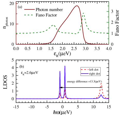
Figure 2: (a) Average photon number(solid brown) and Fano factor(dashed green) as functions of the energy level of right dot, $\varepsilon_{R}$. (b) Local density of states of the DQD for $\varepsilon_{R}=2.6\mu eV$. Other parameter are $\varepsilon_{L}=10\mu eV$, $U_{L}=U_{R}=U_{LR}=0$, $\Gamma_{N}=0.1\mu eV$, $\Gamma_{S}=1\mu eV$, $\mu_{S}=0$, $\hbar\omega_{0}=13.3\mu eV$, $g_{L}=-g_{R}=g_{0}=6.62\times 10^{-2}\mu eV$ and $\kappa=10^{-3}\mu eV$.

In Fig.2(a), we fix the frequency of the resonator to $\hbar\omega_{0}=13.3\mu eV$, and plot the average photon number and the Fano factor of the photons in the resonator as a function of the energy level of right dot, $\varepsilon_{R}$. We see that the average photon number in the resonator shows an asymmetric peak with maximum photon number about $n_{photon}=20$, around $\varepsilon_{R}=2.6\mu eV$, accompanied with a Fano factor slightly lower than $F=1$, corresponding to a sub-Poissonian distribution for the photons in the resonator. A rigorous way to interpret why the lasing happens at these particular gate voltage and resonator frequency and also why the photon peak is asymmetric, is to look at the local density of states(LDOS) of the DQD when it is in equilibrium state and isolated from the resonator and the normal lead. The LDOS can be easily obtained from $-\textrm{Im}[G_{i}^{R}(\omega)]$, where $G_{i}^{R}(\omega)$ is the retarded Green’s function of the dot $i$ which can be calculated by using the Lehmann representation(See AppendixB)(Bruus and Flensberg, 2004). In general, by coupling to a superconducting lead, the peaks in the LDOS of a QD with energies around the chemical potential of the superconducting lead, will be split into two Andreev reflection subgap levels with equal but opposite sign energies(Barański and Domański, 2013). On the other hand, since we have assumed a large positive bias voltage on the left lead, we can expect that the direction of electron tunnelings should be from the left to the right dot. If the energy levels of the two dots are in resonance, we will end up with an electric current originated from resonant Andreev reflections at the interface of the right dot and the superconducting lead(Sun et al., 1999a; Tanaka et al., 2010). However, when the energy levels of the two dots are misaligned, electron tunnelings from left to right dots are assisted by some photon excitation or absorption in the resonator, the frequency of which is equal to the energy difference between the two corresponding LDOS peaks of the left and right dot.

We have plotted the LDOS of the left and right dots in Fig.2(b), for the gate voltage at which the the photon number in the resonator is maximized. We see that the LDOS of left dot, has a large peak around $\hbar\omega\approx 12.3\mu eV$, while the LDOS of the right dot has two main peaks at energies $\hbar\omega\approx\pm 1\mu eV$. It can be deduced that the photon number peak in Fig.2(a), which is for resonator frequency $\hbar\omega_{0}=13.3\mu eV$, is because of electron transitions between the two peaks in the LDOS of DQD by an arrow in Fig.2(b). Interestingly, we see that there is another possible electron transition with energy difference $\hbar\omega\approx 11.3\mu eV$, which we anticipate we can see its lasing effect by tuning the frequency of the resonator to the appropriate frequency. The origin of the asymmetry in the photon peak in Fig.2, can also be deduced from the LDOS by noting that the weight of the Andreev subgap peaks in the LDOS is dependent on the values of the gate voltages.

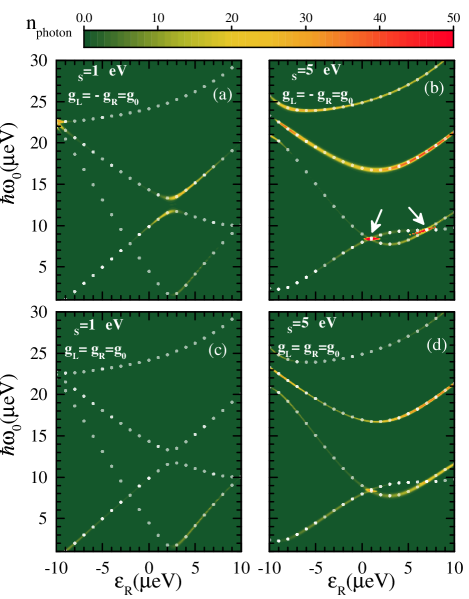
Figure 3: (a)-(d) Average number of photons in the resonator as a function of resonator frequency, $\omega_{0}$, and the energy level of right dot, $\varepsilon_{R}$, for various values of $\Gamma_{S}$ and $g_{L}$ and $g_{R}$. (a) $\Gamma_{S}=1\mu eV$ and $g_{L}=-g_{R}=g_{0},$ (b) $\Gamma_{S}=5\mu eV$ and $g_{L}=-g_{R}=g_{0},$ (c) $\Gamma_{S}=1\mu eV$ and $g_{L}=g_{R}=g_{0},$ (d) $\Gamma_{S}=5\mu eV$ and $g_{L}=g_{R}=g_{0}$. White circles show the energy difference of various peaks in the LDOS at the respective $\varepsilon_{R}$. Other parameters are as in Fig.2.

From the above discussion, it becomes clear that because of the presence of the superconducting lead, there are of course more than one possible lasing frequencies in our model system corresponding to each parameter configuration of the DQD. To see this, we have plotted false color plots of the average photon number in the resonator as a function of $\varepsilon_{R}$ and $\omega_{0}$ in Fig.3. Additionally, we have also calculated energy differences between various LDOS peaks of the system at the different gate voltages, which are shown in Fig.3 by white circles. In Fig.3(a), we consider the same parameter configuration as in Fig.2. We see that lasing happens at various gate voltages as well as in different resonator frequencies. Moreover, as it is expected, the resonator frequencies at which we can see nonzero lasing are exactly equal to the energy differences between various LDOS peaks. It is interesting to note that the regions with nonzero lasing do not follow regular pattern which is mainly because of the fact that positions and heights of the LDOS peaks are non-linear functions of the values of $t_{d}$, $\varepsilon_{R}$, $\varepsilon_{L}$ and $\Gamma_{S}$. Alternatively, this non-linearity can also be seen in the approximate expression which we obtained for the DQD-resonator coupling in Eq.(11).

Next, in Fig.3(b), we investigate the effect of increasing the coupling energy between the right dot and the superconducting lead by setting $\Gamma_{S}=5\mu eV$. Because of increasing the value of $\Gamma_{S}$, the LDOS peaks are renormalized and therefore their energy differences are also changed. Accordingly, the profile of the lasing which should follow these energy differences is changed as well. An important feature in Fig.3(b) is the presence of two points, which are marked by two white arrows. We see that at these points, two branches with nonzero lasing are crossing and, very intriguingly, as a result of this branch crossing the photon number in the resonator is considerably increased. Actually, the crossing of two energy difference branches means that there are two distinct possible electron transitions in the LDOS with exactly the same energy difference. Hence, we can deduce that the sudden increasing of the photon number at these points is due to multiple photon excitation due to the electron transitions from different pairs of peaks in the LDOS. Another feature in Fig.3(b) is that, in the regions around the crossing points, some nonzero lasing occurs at frequencies which are not associated to any energy difference branches. We speculate that these nonzero lasing points are originated from two-level lasing mechanism corresponding to the electron transitions from the two nearby branches(Markus et al., 2003).

So far, in Figs.2 and 3(a) and (b), we have investigated the properties of the lasing state for the situation where the DQD-resonator coupling is asymmetric where $g_{L}=-g_{R}=g_{0}$. However, as we have shown by using some approximative calculations in Sec.II, a spectacular character of the coupling a hybrid DQD to the resonator, is the presence of new coupling mechanism which is dependent on the sum of the coupling strength of each dot to the resonator, $g_{L}+g_{R}$, and therefore, one can obtain lasing in this system even for symmetric DQD-resonator coupling as $g_{L}=g_{R}$. Thus, it is interesting to study the presence of lasing in such symmetric couplings. We have plotted in Figs.3(c) and (d), the same plots as in (a) and (b), except that here we consider the case of $g_{L}=g_{R}=g_{0}$. Here, because the energy configurations of the DQD are not changed, the profile of the energy differences are not altered. However, we see that there are still some nonzero lasing states available for the system in this symmetric coupling configuration. We emphasize that in the case where the DQD is coupled to two normal metals, the DQD-resonator coupling is described only by a term proportional to $g_{L}-g_{R}$, and one could expect that a symmetric DQD-resonator coupling as $g_{L}=g_{R}$, would result in a completely vanishing DQD-resonator coupling and therefore no lasing can happen in such situations.

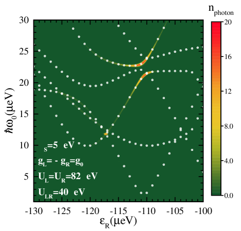
Figure 4: Average number of photons in the resonator as a function of resonator frequency, $\omega_{0}$, and the energy level of right dot, $\varepsilon_{R}$, for the presence of finite electron-electron interactions in DQD. We set $U_{L}=U_{R}=82\mu eV$ and $U_{LR}=40\mu eV$ and other parameters are $\varepsilon_{L}=-110\mu eV$, $\Gamma_{N}=1\mu eV$, $\Gamma_{S}=5\mu eV$, $\mu_{S}=0$, $g_{L}=-g_{R}=g_{0}$ and $\kappa=10^{-3}\mu eV$.

Having realized the presence of the lasing in the coupled hybrid DQD-resonator system as well as its origins and some of its properties, we now study the effect of nonzero electron-electron interactions on the lasing state in our model system. Although, it seems that the presence of finite electron-electron interactions in the hybrid-DQD could suppress the superconducting proximity correlations in the DQD and accordingly could reduce the lasing state, however, previous theoretical and experimental analysis have shown that indeed the electronic transport through a hybrid QD, mainly depends on three energy scales, namely $U/\Gamma_{S}$, $\Gamma_{N}/\Gamma_{S}$ and $t_{d}/\Gamma_{S}$(Doh et al., 2008; Tanaka et al., 2010; Deacon et al., 2010). So, even for large $U$ values, we can expect nonzero conductance through DQD and therefore the presence of lasing in this case is also of no surprise. As a representative example, in Fig.4, we investigate the presence of lasing for a parameter configuration as in Fig.3(b) except that here we consider a large electron-electron interaction in the DQD by setting $U_{L}=U_{R}=82\mu eV$ and $U_{LR}=40\mu eV$, which are roughly similar to the values given in Ref.[Bruhat et al., 2018]. As a result of electron-electron interaction, the energy difference branches are split into many branches (some of them are not shown in Fig.4) and among them, at some particular regions, we can see some nonzero lasing states in various resonator frequencies. Note the large negative gate voltages $\varepsilon_{L}$ and $\varepsilon_{R}$ applied on the DQD in the Fig.4, which are necessary to compensate the large Coulomb interactions in the DQD. Also, note that the energy difference branches are obtained from the energy differences of the roots of the retarded Green’s function, which is calculated for the full interacting system by using the Lehmann representation.

IV Conclusions

In this paper, we studied the possibility of lasing in a single mode electromagnetic resonator which is capacitively coupled to a hybrid DQD. We found that lasing in this system is mediated by electron tunneling between various peaks in the LDOS of the DQD which are induced by Andreev reflections at the DQD-superconducting lead’s interface. Because of this particular lasing mechanism, we showed that the average photon number in the resonator in the lasing state can be further enhanced by multiple electron tunnelings between two different pairs of Andreev reflection peaks with the same energy difference in the LDOS of the DQD. Also, we showed that this system could also exhibit “two-state lasing” which is due to the electron transitions between different Andreev levels in the hybrid DQD with different energy differences.

Appendix A Diagonalization of $\hat{H}_{dqd}^{SC}$

Here, we present the details of steps needed for diagonalizing the Hamiltonian $\hat{H}_{dqd}^{SC}$. In these calculations we disregard the Coulomb interaction in the DQD to simplify our presentation. We start with the matrix representation

$$\hat{H}_{dqd}^{SC}=\hat{\Psi}^{\dagger}(h_{0}+\Gamma_{S}h_{1})\hat{\Psi},$$ (12)

where $\hat{\Psi}^{\dagger}=(\hat{d}_{1,\uparrow}^{\dagger},\hat{d}_{1,\downarrow},\hat{d}_{2,\uparrow}^{\dagger},\hat{d}_{2,\downarrow})$ and

$$h_{0}=\left(\begin{array}[]{cccc}\varepsilon_{1}&0&t_{d}&0\\ 0&-\varepsilon_{1}&0&-t_{d}\\ t_{d}&0&\varepsilon_{2}&0\\ 0&-t_{d}&0&-\varepsilon_{2}\end{array}\right),$$ (13)

and

$$h_{1}=\left(\begin{array}[]{cccc}0&0&0&0\\ 0&0&0&0\\ 0&0&0&1\\ 0&0&1&0\end{array}\right).$$ (14)

We then define four fermionic operators $\hat{\gamma}_{i,\sigma}$ with $i=1,2$ and $\sigma=\uparrow,\downarrow$ such that $\hat{U}^{\dagger}h_{0}\hat{U}$ is diagonal, where $\hat{U}^{\dagger}=(\hat{\gamma}_{1,\uparrow}^{\dagger},\hat{\gamma}_{1,\downarrow},\hat{\gamma}_{2,\uparrow}^{\dagger},\hat{\gamma}_{2,\downarrow})$. This is possible when the operators $\hat{\gamma}_{i,\sigma}$ are related to $\hat{d}_{i,\sigma}$ operators through a Bogoliubov transformation $\hat{U}=K\hat{\Psi}$, where $K$ is given by

$$K=\left(\begin{array}[]{cccc}u&0&v&0\\ 0&u&0&v\\ -v&0&u&0\\ 0&-v&0&u\end{array}\right),$$ (15)

where

$$u(v)=\frac{1}{\sqrt{2}}\sqrt{1\pm\frac{\varepsilon_{L}-\varepsilon_{R}}{\sqrt{(\varepsilon_{L}-\varepsilon_{R})^{2}+4t_{d}^{2}}}}.$$ (16)

Then, we find that $\hat{U}^{\dagger}h_{0}\hat{U}=\textrm{diag}(E_{1},-E_{1},E_{2},-E_{2})$, where $E_{1}(E_{2})=\frac{1}{2}(\varepsilon_{L}+\varepsilon_{R}\pm\sqrt{(\varepsilon_{L}-\varepsilon_{R})^{2}+4t_{d}^{2}})$.

To take into account the effect of the second term of Eq.(12), we perform a first order perturbation on the eigenfunctions of the matrix $h_{0}$ with respect to the perturbation term $\Gamma_{S}h_{1}$. These perturbed eigenfunctions can be represented by

$$\hat{U}=(K+\Gamma_{S}K^{\prime})\hat{\Psi},$$ (17)

where

$$K^{\prime}=\hskip 199.16928pt$$

$$\left(\begin{array}[]{cccc}{\scriptstyle 0}&{\scriptstyle\frac{uv^{2}}{2E_{1}}-\frac{uv^{2}}{E_{1}+E_{2}}}&{\scriptstyle 0}&{\scriptstyle\frac{v^{3}}{2E_{1}}+\frac{u^{2}v}{E_{1}+E_{2}}}\\ {\scriptstyle-\frac{uv^{2}}{2E_{1}}+\frac{uv^{2}}{E_{1}+E_{2}}}&{\scriptstyle 0}&{\scriptstyle-\frac{v^{3}}{2E_{1}}-\frac{u^{2}v}{E_{1}+E_{2}}}&{\scriptstyle 0}\\ {\scriptstyle 0}&{\scriptstyle\frac{u^{2}v}{E_{2}+E_{1}}-\frac{u^{2}v}{2E_{2}}}&{\scriptstyle 0}&{\scriptstyle\frac{uv^{2}}{E_{2}+E_{1}}+\frac{u^{3}}{2E_{2}}}\\ {\scriptstyle-\frac{u^{2}v}{E_{2}+E_{1}}+\frac{u^{2}v}{2E_{2}}}&{\scriptstyle 0}&{\scriptstyle-\frac{uv^{2}}{E_{2}+E_{1}}-\frac{u^{3}}{2E_{2}}}&{\scriptstyle 0}\end{array}\right).$$ (22)

Now, it is straightforward to show by matrix multiplication that the first order correction to the eigenenergies of $\hat{H}_{dqd}^{SC}$ is zero and its diagonalized form in terms of $\hat{\gamma}_{i,\sigma}$ operators can be given by

$$\hat{\widetilde{H}}_{dqd}^{SC}=U^{\dagger}\hat{H}_{dqd}^{SC}U=\sum_{i,\sigma}E_{i}\hat{\gamma}_{i,\sigma}^{\dagger}\hat{\gamma}_{i,\sigma}+\mathcal{O}(\Gamma_{S}^{2}).$$ (23)

The main benefit which we can obtain from above calculations is that we can apply the same unitary transformation $U$ on the DQD-resonator coupling Hamiltonian $\hat{H}_{ph-dqd}$ to obtain its representation in the terms of $\hat{\gamma}_{i,\sigma}$ operators as:

$$\hat{\widetilde{H}}_{ph-dqd}=-\sum_{\sigma}(\hat{a}+\hat{a}^{\dagger})[(g_{L}-g_{R})\hskip 56.9055pt$$

$$\times\left[-uv\hat{\gamma}_{1,\sigma}^{\dagger}\hat{\gamma}_{2,\sigma}+\Gamma_{S}uv\left(\frac{u^{2}}{2E_{2}}+\frac{v^{2}}{2E_{1}}\right)\hat{\gamma}_{1,\sigma}^{\dagger}\hat{\gamma}_{2,-\sigma}^{\dagger}\right]$$

$$\hskip 28.45274pt-(g_{L}+g_{R})\left[\Gamma_{S}\frac{uv}{E_{1}+E_{2}}\hat{\gamma}_{1,\sigma}^{\dagger}\hat{\gamma}_{2,-\sigma}^{\dagger}\right]]+h.c.$$ (24)

Appendix B Lehmann representation of $G_{i}^{R}(\omega)$

As we discussed in Sec.III, to the linear order of interaction between the DQD and the resonator and in the weak coupling regime, it is reasonable to expect that the possible lasing frequencies in the resonator can be explained by electron transitions between various peaks in the LDOS of the DQD when it is isolated from the resonator and also from the normal lead. It is convenient to to calculate the LDOS of the DQD from $-\textrm{Im}[G_{i}^{R}(\omega)]$, where $G_{i}^{R}(\omega)$ is the retarded Green’s function of the dot $i$ and can be calculated from the Lehmann representation.(Bruus and Flensberg, 2004) In the following we briefly summarize the main steps needed to calculate the retarded Green’s function of the DQD.

Our starting point is the Hamiltonian of the DQD

$$\hat{H}_{dqd}^{SC}= \sum_{\alpha\sigma}\varepsilon_{\alpha}\hat{n}_{\alpha,\sigma}+U_{\alpha}\hat{n}_{\alpha,\uparrow}\hat{n}_{\alpha,\downarrow}+U_{LR}\hat{n}_{L}\hat{n}_{R}$$

$$+t_{d}\sum_{\sigma}(d_{R,\sigma}^{\dagger}d_{L,\sigma}+h.c)+\Gamma_{S}(\hat{d}_{R,\uparrow}^{\dagger}\hat{d}_{R,\downarrow}^{\dagger}+h.c).$$ (25)

To proceed, we need the eigenstates and the eigenenergies of Eq.(25), which as we discussed in Sec.II, obtaining an analytical expression for its eigenstates is practically impossible. Nevertheless, we can rely on numerical methods and express the numerically calculated eigenstates of Eq.(25) and their corresponding eigenenergies by $\bigl{|}n\bigr{\rangle}$ and $\mathcal{E}_{n}$ where $n=1,2,\cdots,16$. Having the eigenspectrum of the Hamiltonian of the DQD, we can then calculate the retarded Green’s function of the DQD from

$$G_{i,\sigma}^{R}(\omega)=\frac{1}{Z}\sum_{m,m^{\prime}}\frac{\bigl{\langle}m\bigr{|}d_{i,\sigma}\bigl{|}m^{\prime}\bigr{\rangle}\bigl{\langle}m^{\prime}\bigr{|}d_{i,\sigma}^{\dagger}\bigl{|}m\bigr{\rangle}}{\omega+\mathcal{E}_{m}-\mathcal{E}_{m^{\prime}}+i\eta}\left(e^{-\beta\mathcal{E}_{m}}+e^{-\beta\mathcal{E}_{m^{\prime}}}\right),$$ (26)

where $Z=\sum_{m}e^{-\beta\mathcal{E}_{m}}$, $\eta$ is an infinitesimal positive constant and $\beta$ is the inverse temperature.

References

- Mu and Savage (1992) Y. Mu and C. Savage, Phys. Rev. A 46, 5944 (1992).
- Ginzel et al. (1993) C. Ginzel, H.-J. Briegel, U. Martini, B.-G. Englert, and A. Schenzle, Phys. Rev. A 48, 732 (1993).
- Pellizzari and Ritsch (1994a) T. Pellizzari and H. Ritsch, Phys. Rev. Lett. 72, 3973 (1994a).
- Pellizzari and Ritsch (1994b) T. Pellizzari and H. Ritsch, J. Mod. Opt. 41, 609 (1994b).
- An et al. (1994) K. An, J. J. Childs, R. R. Dasari, and M. S. Feld, Phys. Rev. Lett. 73, 3375 (1994).
- Jones et al. (1999) B. Jones, S. Ghose, J. P. Clemens, P. R. Rice, and L. M. Pedrotti, Phys. Rev. A 60, 3267 (1999).
- Löffler et al. (1997) M. Löffler, G. M. Meyer, and H. Walther, Phys. Rev. A 55, 3923 (1997).
- Karlovich and Kilin (2001) T. Karlovich and S. Y. Kilin, Opt. Spectrosc. 91, 343 (2001).
- McKeever et al. (2003) J. McKeever, A. Boca, A. D. Boozer, J. R. Buck, and H. J. Kimble, Nature 425, 268 (2003).
- Yoshie et al. (2004) T. Yoshie, A. Scherer, J. Hendrickson, G. Khitrova, H. Gibbs, G. Rupper, C. Ell, O. Shchekin, and D. Deppe, Nature 432, 200 (2004).
- Florescu et al. (2004) L. Florescu, S. John, T. Quang, and R. Wang, Phys. Rev. A 69, 013816 (2004).
- Aoki et al. (2006) T. Aoki, B. Dayan, E. Wilcut, W. P. Bowen, A. S. Parkins, T. Kippenberg, K. Vahala, and H. Kimble, Nature 443, 671 (2006).
- Lougovski et al. (2007) P. Lougovski, F. Casagrande, A. Lulli, and E. Solano, Phys. Rev. A 76, 033802 (2007).
- Florescu (2008) L. Florescu, Phys. Rev. A 78, 023827 (2008).
- Kim et al. (2008) H.-J. Kim, A. H. Khosa, H.-W. Lee, and M. S. Zubairy, Phys. Rev. A 77, 023817 (2008).
- Ritter et al. (2010) S. Ritter, P. Gartner, C. Gies, and F. Jahnke, Opt. Express 18, 9909 (2010).
- Reithmaier et al. (2004) J. P. Reithmaier, G. Sek, A. Löffler, C. Hofmann, S. Kuhn, S. Reitzenstein, L. Keldysh, V. Kulakovskii, T. Reinecke, and A. Forchel, Nature 432, 197 (2004).
- Reitzenstein et al. (2008) S. Reitzenstein, C. Böckler, A. Bazhenov, A. Gorbunov, A. Löffler, M. Kamp, V. Kulakovskii, and A. Forchel, Opt. Express 16, 4848 (2008).
- Nomura et al. (2009) M. Nomura, N. Kumagai, S. Iwamoto, Y. Ota, and Y. Arakawa, Opt. Express 17, 15975 (2009).
- Nomura et al. (2010) M. Nomura, N. Kumagai, S. Iwamoto, Y. Ota, and Y. Arakawa, Nat. Phys. 6, 279 (2010).
- Ledentsov (2010) N. Ledentsov, Semicond. Sci. Technol. 26, 014001 (2010).
- Liu et al. (2011) H. Liu, T. Wang, Q. Jiang, R. Hogg, F. Tutu, F. Pozzi, and A. Seeds, Nat. Photonics 5, 416 (2011).
- Marthaler et al. (2011) M. Marthaler, Y. Utsumi, D. S. Golubev, A. Shnirman, and G. Schön, Phys. Rev. Lett. 107, 093901 (2011).
- Jin et al. (2011) P.-Q. Jin, M. Marthaler, J. H. Cole, A. Shnirman, and G. Schön, Phys. Rev. B 84, 035322 (2011).
- Toida et al. (2013) H. Toida, T. Nakajima, and S. Komiyama, Phys. Rev. Lett. 110, 066802 (2013).
- Liu et al. (2015) Y.-Y. Liu, J. Stehlik, C. Eichler, M. Gullans, J. M. Taylor, and J. Petta, Science 347, 285 (2015).
- Karlewski et al. (2016) C. Karlewski, A. Heimes, and G. Schön, Phys. Rev. B 93, 045314 (2016).
- Stehlik et al. (2016) J. Stehlik, Y.-Y. Liu, C. Eichler, T. Hartke, X. Mi, M. Gullans, J. Taylor, and J. Petta, Phys. Rev. X 6, 041027 (2016).
- Astafiev et al. (2007) O. Astafiev, K. Inomata, A. Niskanen, T. Yamamoto, Y. A. Pashkin, Y. Nakamura, and J. Tsai, Nature 449, 588 (2007).
- Hauss et al. (2008) J. Hauss, A. Fedorov, C. Hutter, A. Shnirman, and G. Schön, Phys. Rev. Lett. 100, 037003 (2008).
- Grajcar et al. (2008) M. Grajcar, S. Van der Ploeg, A. Izmalkov, E. Ilichev, H.-G. Meyer, A. Fedorov, A. Shnirman, and G. Schön, Nature physics 4, 612 (2008).
- André et al. (2009) S. André, V. Brosco, M. Marthaler, A. Shnirman, and G. Schön, Phys. Scr. 2009, 014016 (2009).
- Sun et al. (1999a) Q.-f. Sun, J. Wang, and T.-h. Lin, Phys. Rev. B 59, 3831 (1999a).
- Sun et al. (1999b) Q.-f. Sun, J. Wang, and T.-h. Lin, Phys. Rev. B 59, 13126 (1999b).
- Sun et al. (2001) Q.-f. Sun, H. Guo, and T.-h. Lin, Phys. Rev. Lett. 87, 176601 (2001).
- Cuevas et al. (2001) J. C. Cuevas, A. Levy Yeyati, and A. Martín-Rodero, Phys. Rev. B 63, 094515 (2001).
- Nurbawono et al. (2010) A. Nurbawono, Y. P. Feng, and C. Zhang, Phys. Rev. B 82, 014535 (2010).
- Barański and Domański (2013) J. Barański and T. Domański, J. Phys.: Condens. Matter 25, 435305 (2013).
- Weymann and Wójcik (2015) I. Weymann and K. Wójcik, Phys. Rev. B 92, 245307 (2015).
- Bruhat et al. (2016) L. Bruhat, J. Viennot, M. Dartiailh, M. Desjardins, T. Kontos, and A. Cottet, Phys. Rev. X 6, 021014 (2016).
- Rastelli and Governale (2019) G. Rastelli and M. Governale, Phys. Rev. B 100, 085435 (2019).
- Bruhat et al. (2018) L. E. Bruhat, T. Cubaynes, J. J. Viennot, M. C. Dartiailh, M. M. Desjardins, A. Cottet, and T. Kontos, Phys. Rev. B 98, 155313 (2018).
- Trocha and Barnaś (2014) P. Trocha and J. Barnaś, Phys. Rev. B 89, 245418 (2014).
- Nigg et al. (2015) S. E. Nigg, R. P. Tiwari, S. Walter, and T. L. Schmidt, Physical Review B 91, 094516 (2015).
- Gullans et al. (2018) M. J. Gullans, J. M. Taylor, and J. R. Petta, Phys. Rev. B 97, 035305 (2018).
- Agarwalla et al. (2019) B. K. Agarwalla, M. Kulkarni, and D. Segal, Phys. Rev. B 100, 035412 (2019).
- Pfaller et al. (2013) S. Pfaller, A. Donarini, and M. Grifoni, Phys. Rev. B 87, 155439 (2013).
- Mendes and Mora (2016) U. C. Mendes and C. Mora, Phys. Rev. B 93, 235450 (2016).
- Breuer et al. (2002) H.-P. Breuer, F. Petruccione, et al., The theory of open quantum systems (Oxford University Press on Demand, 2002).
- Johansson et al. (2013) J. R. Johansson, P. D. Nation, and F. Nori, Comput. Phys. Commun. 184, 1234 (2013).
- Doh et al. (2008) Y.-J. Doh, S. D. Franceschi, E. P. Bakkers, and L. P. Kouwenhoven, Nano letters 8, 4098 (2008).
- Liu et al. (2014) Y.-Y. Liu, K. D. Petersson, J. Stehlik, J. M. Taylor, and J. R. Petta, Phys. Rev. Lett. 113, 036801 (2014).
- Bruus and Flensberg (2004) H. Bruus and K. Flensberg, Many-body quantum theory in condensed matter physics: an introduction (Oxford university press, 2004).
- Tanaka et al. (2010) Y. Tanaka, N. Kawakami, and A. Oguri, Phys. Rev. B 81, 075404 (2010).
- Markus et al. (2003) A. Markus, J. Chen, C. Paranthoen, A. Fiore, C. Platz, and O. Gauthier-Lafaye, Appl. Phys. Lett. 82, 1818 (2003).
- Deacon et al. (2010) R. Deacon, Y. Tanaka, A. Oiwa, R. Sakano, K. Yoshida, K. Shibata, K. Hirakawa, and S. Tarucha, Phys. Rev. Lett. 104, 076805 (2010).