The Average Physical Properties of A-G Stars Derived from uvby-H Strömgren-Crawford Photometry as the Basis for a Spectral-Classification Synthetical Approach
Abstract
We have revisited and updated the Strömgren colour and colour-index distributions of A, F and early G-type main sequence stars. For this aim, we selected 7054 dwarf stars along with 65 MK standard stars within the same spectral range but covering all luminosity classes. The standard stars were selected following the MK mandate strictly, using spectra taken at classification resolution recorded on photographic plates. We used the colours of these stars to determine the effective temperature and surface gravity. After correcting for systematic offsets using fundamental parameters and considering a few exceptions, we find an one-to-one correspondence, among MK spectral types, Strömgren photometry, and their associated physical properties.
We have applied a principal component analysis to the mean Strömgren indices for dwarf stars complemented by MK standards for higher luminosity classes. We have used the projections to introduce three new photometric metaindices, namely SM1, SM2, and SM3. We have defined a 3D-box, which allowed us to segregate dwarf stars from bright giants and supergiant stars, with the aid of the metaindices. Two of the planes show that the projections of dwarfs and supergiants are ordered by temperature; however, the temperature dependence for the supergiants is not as well defined as for the dwarfs. Following the MK Process, we were able to form an automatic classifier. We present some applications and assigned synthetical spectral types. We suggest that our metaindices formalism allows the extension of Strömgren photometric outside its original mandate (i.e., later types), without requiring the introduction of additional photometric filters.
keywords:
stars: fundamental parameters – stars: statistics – Galaxy: solar neighbourhood – techniques: photometric – standards1 Introduction
The Morgan-Keenan system (MK, hereafter) is an autonomous and self-consistent approach for stellar spectral classification. It relies on a well-defined set of standard stars, chosen on the basis of the phenomenology of spectral lines, blends and bands, according to a general progression of spectral type (abscissa) and luminosity (ordinate) (e.g., Morgan & Keenan, 1973; Mihalas, 1984; Morgan, 1984; Garrison, 1985; Gray & Corbally, 2009); hence, the standard stars define a two-dimensional grid of well separated spectral types and luminosity classes. To classify a given star, the classifier compares and interpolates its spectrum across the grid, considering the particular features to a class, but paying attention to the whole spectrum. The system was defined for Population I stars using the blue-violet region of the stellar spectrum. On the other hand, the MK Process (e.g., Morgan, 1984) as a methodology for classification has been successfully extended to other regions of the electromagnetic spectrum (Gray & Corbally, 2009). As any properly defined classification system, one of the main uses of the MK system is to separate rare or peculiar objects from the broad population of “normal stars" (e.g., Morgan, 1984; Garrison, 1985); notwithstanding, one of the most creative and powerful applications of the MK system was implemented by Morgan et al. (1952, 1953). Morgan et al. carried out a comprehensive search for galactic OB stars to map their distribution. Aided with spectroscopic parallaxes and correcting for extinction, Morgan and his collaborators were able to outline the spiral structure of the Galaxy, for the first time.
There have been several attempts to apply the MK system automatically. Manteiga et al. (2009) presented a list of spectral line-strengths, band fluxes and their ratios of MK standards; however, a closer advance to the emulate a classifier using the MK system was developed by Gray & Corbally (2014), who generated a computer program to classify stellar spectra by direct comparison with a set of MK standards.
1.1 Intermediate band photometry and stellar classification

Early on, it was realized that stellar photometry provided a complementary quantitative approach to spectral classification (e.g., Johnson & Morgan, 1953; Strömgren, 1966; Crawford, 1984; Smriglio et al., 1990; Crawford, 1994). The original complementary found between the MK types and stellar photometry (Johnson & Morgan, 1953; Strömgren, 1966) has become clearer as we have gained access larger data bases of stellar measurements and spectral classifications, and more realistic stellar atmosphere models.
Figure 1 shows the transmission curves (in dashed lines) for each of the filters that define (e.g., Straižys, 1992; Bessell, 2005) the photometric system introduced by Bengt Strömgren during the 1950s (See review by Strömgren, 1966). In general, intermediate-band photometric systems are able to reproduce the results derived from low resolution spectroscopy. Strömgren carefully configure the set of filters to define this photometric system, considering the broad stellar spectral properties, his aim was to closely match the MK classification system. Strömgren introduced colors and two indices resulting after the linear combination of colors. The color is sensitive to temperature but insensitive to metallicity (because of small and comparable line blanketing in and ), the color is very sensitive to metallicity particularly for F and G stars due to the large blanketing in and much smaller blanketing in , while the band reproduces Johnson’s band. The indices and measure physical properties which are unaccessible employing broad band filters: the measures the Balmer discontinuity, while the estimates line blanketing of A-G type stars, respectively. The Strömgren photometric system was originally designed to approximate spectral classifications for A2 to G2 stars. Successful extensions to the range of applicability to earlier or later types out of the aforemetioned range, have been achieved by introducing extra filters. For example the index introduced by Crawford (1958) to include stars earlier than A2. This extended system is called the uvby- Strömgren-Crawford Photometric System (Crawford & Strömgren, 1966). Anthony-Twarog et al. (1991) introduced the index design to cover the Ca II and lines, this extension allowed the consideration of metal poor dwarfs and red giants.
In Figure 1 the Å, Å, Å and Å filter passbands are overpplotted onto a A0 V stellar spectrum generated with CHORIZOS (Maíz-Apellániz, 2004, see §4, below) from a Kurucz model (Kurucz, 2004) while the uvby filter profiles are from The Isaac Newton Group filter database. Only the filter contains a strong absorption line, the H Balmer. The other filters do not contain very strong lines up to spectral type G0. Strömgren photometry is more sensitive to subtle variations in spectral energy distribution than broadband photometry, but less time consuming than spectroscopy.
Recently, Monguió et al. (2014) introduced a complex classification scheme based on MK standards and developed an automatic method for deriving the stellar physical parameters from Strömgren photometry. This attempt responded, at least partially, to the concerns raised by sticklers who hold that spectral types assigned from photometric are improper, because they are generated outside the MK mandate (e.g., Garrison, 1985), and, therefore, not accurate enough. Nevertheless, below, we show that the stellar physical properties derived photometrically approximate the physical basis of the MK sequence (See §2.4 in Gray & Corbally, 2009); therefore, we can extend the photometric approach to spectral classification based on the MK process, and provide complementary classifications to large numbers of faint stars, for which proper spectral inspection would be too time consuming.
Also we introduce a new photometry-based classification scheme, which is able to approximate MK types for normal stars. Our scheme is based on a principal component analysis (PCA) of the Strömgren indices (cf., Steindling et al., 2001). With the aid of our classification scheme we are able to segregate dwarf from supergiants, and assign spectral types automatically. (Terranegra et al., 1994) presented a simpler photometrically approach to spectral classification using Strömgren indexes.
This paper is organized as follows: §1 we give specific details on the MK system, the MK Process and the -H Strömgren-Crawford Photometry. In §2 we describe the selection of the sample and the reddening corrections; the properties of the observed photometry are presented in §3; the derivation of physical parameters is given in §4; §4.1 describes how we derived a transformation to match our results with fundamental effective temperatures effective temperature and also is presented a comparison with standard stars; results are listed in §4; in §5, we show Strömgren photometric indices space allows a reduction in dimension; hence, the main sequence can be reduced to straight line using a projection generated by principal component analysis (PCA). We also present applications of the proposed classification scheme. In last section (§6) we present our conclusions.
2 Sample selection
A recent compilation of 298 639 -H photometric measurements of 60 668 stars by Paunzen (2015), almos includes the fully earlier catalogue by Hauck & Mermilliod (1998), which contains 63 313 stars. Although, Paunzen’s compilation has reprocessed all the previous measurements and is much larger than Hauck & Mermilliod’s, due to the inclusion of CCD-based photometry, we found that analysis using either compilation were indistinguishable; therefore, we opted for the original compilation by Hauck & Mermilliod (1998). MK Spectral classifications were taken from the ongoing compilation by Skiff (2014), and parallaxes from HIPPARCOS (Perryman et al., 1997).
A preselection was done, considering that stars earlier than A0 V are not well represented in Paunzen (2015) compilation, see also Figure 2 in Sowell et al. (2007). The apparent absence of these stars can be explained by their short lifetimes and by their position within the Galaxy: stars earlier than A0 are highly massive and are often found in high extinction regions. On the other hand, we considered stars three types later than G2 V just for completeness; hence, we explored spectral classes outside the original mandate of the Strömgren system.
We have given preference to the classifications published in the University of Michigan Catalogue of Two-Dimensional Spectral Types for the HD Stars, Volumes 1–5 (Houk, & Cowley, 1975; Houk, & Fesen, 1978; Houk, 1982; Houk, & Smith-Moore, 1988; Houk, & Swift, 1999). The first reason is that the classifications were done following the MK system and mandate strictly (objective prism spectra on photographic plates). The second, most important, reason is that 96% of the classification provided in the Michigan Catalogues were assigned by a single expert classifier, Nancy Houk (Caballero-Nieves et al., 2007; Sowell et al., 2007). Hence, 86% MK of the classifications included in our study were taken from the Michigan Catalogues. Spectra of bright stars were saturated in the plates used by Houk, classifications to those stars were provided independently Robert F. Garrison, a list of 348 classifications assigned by R. F. Garrison using slit spectra on photographic plates are presented in Table 8 in Sowell et al. (2007).
In the MK system peculiar stars are marked by the letter "p" or the abbreviation "pec", or by the lack of convergence to a single type and luminosity class. Peculiarities are indicated by the presence of strong metallic lines, or by different types using hydrogen lines and other discrepant spectral features; hence, we have excluded peculiar stars including Am, Ap or any chemically peculiar (CP) star. Moreover, we checked that none of the CP candidate stars published by Renson & Manfroid (2009) were included.
For the rest of the stars included in this paper, we revised the sources to avoided MK-like classifications assigned by the modeling of the stellar spectral energy distribution (e.g., Ahn et al., 2012). We have made an effort to include only stars with the highest quality types assigned according to MK system. Our final sample contains 7054 normal star with full spectral classifications (single spectral type and luminosity class) covering from A0 V to G5 V, having accurate -H Strömgren-Crawford photometry, and a magnitude limit of mag.
We compared Houk with those derived from digital spectra by Gray, Napier, & Winkler (2001); Gray et al. (2003, 2006). Figure 2 shows the comparison between these classifiers. A slight trend is noted where early-type stars classified by Gray, Napier, & Winkler appear to be slightly later than the types by Houk. On the other hand, stars classified by Houk around G0 are systematically later than those of Gray, Napier, & Winkler (2001); Gray et al. (2003, 2006). E. Mamajek (Personal communication) noted that Houk chose the star HD 114710 as the standard for the G2 V class; nevertheless, this star was later revised to G0 V (e.g., Gray, Napier, & Winkler, 2001; Frasca et al., 2009); hence, the main source of discrepancy seen in Figure 2 is generated by selected grid of standard employed by each study. However, we will see below a clear progression of the spectral properties and the photometric and physical properties of the stars. A note regarding the definition of G2 V class and the Sun as a standard star is provided by E. Mamajeck,111http://www.pas.rochester.edu/~emamajek/memo_G2V.html: a more philosophical, discussion on the usage and abusage of MK mandate is provided by Garrison (1985).
| Identifier | Spectral type | Source | |||
|---|---|---|---|---|---|
| HD 196379 | A9 II | MK73 | 0.236 | 0.091 | 1.4810 |
| HD 23585 | F0 V | MK78 | 0.190 0.005 | 0.178 0.010 | 0.717 0.008 |
| HD 220392 | F0 IV | GG89 | 0.147 0.003 | 0.187 0.002 | 0.967 0.001 |
| 57 Tau | F0 IV | MK78 | 0.171 0.002 | 0.194 0.005 | 0.770 0.003 |
| CMi | F0 IIIb | GG89 | 0.132 0.005 | 0.193 0.002 | 1.007 0.007 |
| 38 Cnc | F0 IIIb | GG89 | 0.153 | 0.180 | 0.995 |
| Leo | F0 III∗ | MK78 | 0.196 | 0.169 | 0.986 |
| HD 6130 | F0 II | MK73 | 0.362 0.002 | 0.069 0.001 | 1.179 0.013 |
| Lep | F0 Ib∗ | MK78 | 0.139 0.001 | 0.149 0.002 | 1.503 0.004 |
| Cas | F0 Ia | MK78 | 0.492 0.002 | -0.002 0.011 | 1.438 0.012 |
| HD 113139 | F2 V∗ | MK78 | 0.244 0.002 | 0.170 0.003 | 0.576 0.003 |
| 32 Tau | F2 IV | GG89 | 0.225 | 0.152 | 0.660 |
| Cas | F2 III | GG89 | 0.216 | 0.177 | 0.785 |
| Aql | F2 Ib | GG89 | 0.420 0.005 | 0.069 0.006 | 1.449 0.012 |
| Sco | F2 Ia | MK78 | 0.337 | 0.107 | 1.459 |
| HD 26015 | F3 V | MK78 | 0.270 | 0.164 | 0.488 |
| 20 CVn | F3 III | MK78 | 0.176 0.003 | 0.232 0.005 | 0.915 0.003 |
| HD 27524 | F5 V | MK73 | 0.285 0.002 | 0.161 0.002 | 0.461 0.004 |
| CMi | F5 IV-V | MK78 | 0.272 0.000 | 0.167 0.000 | 0.532 0.000 |
| 48 Gem | F5 III-IV | MK78 | 0.246 | 0.170 | 0.786 |
| HD 186155 | F5 II-III | MK78 | 0.264 0.003 | 0.203 0.002 | 0.718 0.005 |
| Per | F5 Ib∗ | MK78 | 0.301 0.004 | 0.196 0.004 | 1.073 0.001 |
| HD 10494 | F5 Ia | MK78 | 0.875 | -0.026 | 1.458 |
| HD 30652 | F6 V∗ | MK73 | 0.298 0.002 | 0.163 0.002 | 0.415 0.004 |
| Tri | F6 IV | MK73 | 0.316 | 0.156 | 0.501 |
| HD 160365 | F6 III | MK73 | 0.374 0.002 | 0.162 0.003 | 0.555 0.003 |
| HD 222368 | F7 V | MK53 | 0.330 0.002 | 0.163 0.004 | 0.399 0.003 |
| HD 27808 | F8 V | MK78 | 0.338 0.002 | 0.172 0.005 | 0.382 0.007 |
| HD 217096 | F8 III-IV | MK73 | 0.366 0.006 | 0.188 0.002 | 0.489 0.013 |
| Peg | F8 III | MK78 | 0.390 | 0.187 0.002 | 0.461 0.001 |
| Cyg | F8 Ib | MK78 | 0.393 0.004 | 0.296 0.005 | 0.884 0.002 |
| CMa | F8 Ia∗ | MK78 | 0.375 | 0.322 | 0.929 |
| HD 27383 | F9 V | MK73 | 0.352 0.003 | 0.192 0.003 | 0.370 0.005 |
| HD 109358 | G0 V∗ | K76/K85 | 0.385 | 0.182 0.001 | 0.298 0.006 |
| Boo | G0 IV∗ | MK78/K85 | 0.374 0.003 | 0.203 0.003 | 0.488 0.020 |
| Psc | G0III | MK73 | 0.440 0.003 | 0.221 0.010 | 0.439 0.013 |
| Cam | G0 Ib-IIa | MK53/K85 | 0.559 0.010 | 0.328 0.006 | 0.485 0.011 |
| Per | G0 Ib | MK53/K85 | 0.616 0.003 | 0.273 0.007 | 0.545 0.015 |
| Aqr | G0 Ib | MK53/K85 | 0.512 0.001 | 0.325 0.001 | 0.566 0.016 |
| HD 91629 | G0 Ia | MK73 | 0.481 | 0.256 0.004 | 0.609 0.008 |
| HD 18391 | G0 Ia FeI | MK53 | 1.386 | 0.333 | 0.411 |
| HD 101947 | G0 0-Ia FeI | K85 | 0.468 0.015 | 0.279 0.011 | 0.599 0.053 |
| HD 27836 | G1 V | MK73 | 0.384 0.003 | 0.200 0.002 | 0.330 0.006 |
| Her | G1 IV∗ | MK73/K85 | 0.413 0.003 | 0.207 0.004 | 0.408 0.005 |
| Leo | G1 II | K76/K85 | 0.507 0.005 | 0.276 0.004 | 0.452 0.009 |
| Vir | G2 IV | K76/K85 | 0.439 0.003 | 0.207 0.003 | 0.383 0.003 |
| 84 Her | G2 IIIb | K76/K85 | 0.424 0.005 | 0.219 0.005 | 0.452 0.004 |
| Dra | G2 Ib-IIa | K85 | 0.608 0.004 | 0.323 0.003 | 0.423 0.006 |
| Aqr | G2 Ib | K53/K85 | 0.588 0.007 | 0.384 0.007 | 0.447 0.007 |
| HD 96746 | G2 Iab | K76 | 0.574 | 0.306 | 0.534 |
| R Pup | G2 0-Ia | K76/K85 | 0.701 0.003 | 0.253 0.009 | 0.868 0.023 |
| HD 10307 | G2 V | MK53 | 0.389 | 0.198 0.005 | 0.348 0.011 |
| HD 3421 | G2.5 IIa | K85 | 0.555 | 0.322 | 0.375 |
| 37 LMi | G2.5 IIa | K85 | 0.512 0.002 | 0.294 0.005 | 0.478 0.003 |
| HD 186427 | G3 V | MK85 | 0.416 | 0.226 | 0.354 |
| 22 Vul | G3 Ib-IIp | MK73 | 0.652 | 0.363 | 0.351 |
| Sct | G4 IIa | K76/K85 | 0.709 0.006 | 0.352 0.005 | 0.430 0.013 |
| HD 20630 | G5 V∗ | MK53/K85 | 0.419 0.003 | 0.235 0.005 | 0.307 0.003 |
| Her | G5 IV | K53/K85 | 0.468 0.005 | 0.271 0.010 | 0.407 0.007 |
| HD 27022 | G5 IIb | K76/K85 | 0.511 0.001 | 0.286 0.004 | 0.405 0.003 |
| Gem | G5 Ib-IIa | K76 | 0.575 | 0.361 | 0.372 |
| 25 Gem | G5 Ib | MK53 | 0.661 | 0.430 | 0.330 |
| 9 Peg | G5 Ib | MK53/K85 | 0.706 0.002 | 0.480 0.007 | 0.349 0.008 |
| HD 49396 | G5 Iab | K76 | 0.647 0.002 | 0.457 0.007 | 0.422 0.008 |
| HD 217476 | G5 0-Ia | K76 | 0.803 | 0.224 | 1.039 |
Grid of MK standards set up by López-Cruz (1991) with photometric measurements taken from Hauck & Mermilliod (1998). These stars were selected by López-Cruz using photographic plates taken at classification resolution, with strict observance of the MK mandate. They conform a smooth progression of types and luminosity classes. In column 3, the sources are indicated as follows: MK53 (Johnson & Morgan, 1953), MK73 (Morgan & Keenan, 1973), MK78 (Morgan et al., 1978), K76 (Keenan & McNeil, 1976), K85 (Keenan & Yorka, 1985), and GG89 (Gray & Garrison, 1989). The starts marked by ∗ in column 2, were defined as anchor points by Garrison (1994).

2.0.1 MK Standards
In order to extend our analysis to higher luminosity classes and observe consistency with the MK Process, we have included in this study a grid of 65 MK standard stars selected by OL-C (López-Cruz, 1991, see Table 1 and §4.2 below). These stars were observed with a dispersion of 65Å/mm on photographic plates. The plates were taken with similar spectrographs (in Chile or Mexico) and were processed in the same manner. They are, now, part of the Garrison Archive at the University of Toronto. The original idea was to provide a densely populated MK grid for visual spectral classification. Each spectrum was examined and checked to follow a smooth progression both in spectral type and luminosity class. Table 1, also includes 10 "anchor points" as defined by Garrison (1994). These anchor points are the most stable standard MK standards, as their spectral types have not changed throughout the historical revisions of the MK classification system. Those 10 anchor points are marked by an asterisk on column 2. Nevertheless, owing to the powerful interpolating ability of the eye-brain neurological complex, the trained classifier is able to assigned accurate types, even in the presence of large gaps in the grid of standard stars. The grid defined by the stars in Table 1 was used to search for F supergiant stars at high galactic latitude (López-Cruz, 1991; López-Cruz & Garrison, 1993; Garrison & López-Cruz, 1993). Due to the intrinsic properties of evolved stars, there are not enough MK classified stars to generate an statistical analysis, the situation is complicated by spectral-type variations. The situation can be grasp in Figure 2 Sowell et al. (2007). Hence, we resorted to the MK standard stars in Table 1 to extend our analysis to evolved star, this is just a first order approximation. Appendix A in Gray & Corbally (2009) provides updated MK standard stars that can complement our Table.
2.1 Reddening correction
Understanding the local interstellar reddening is very important in the derivation of the intrinsic color calibration and hence the other indices and as well (hereafter the subscript 0 means that the color or index re reddening free or has been derredened). The nearest interstellar dust patches are at about 70 pc from the Sun; this region devoid of dust is commonly identified with the Local Hot Bubble. Indeed, several investigations indicate that the effects of interstellar reddening are negligible for stars closer than 70 pc from the Sun (e.g., Tinbergen, 1982; Leroy, 1999; Holmberg et al., 2007; Luck & Heiter, 2007). On the other hand, the study of Reis et al. (2011) uses the same classical methods for estimating color excess employed in this paper. Reis et al. results agree with those of Perry, & Johnston (1982), suggesting that the effects of interstellar reddening may be ignored for stars as far as 80 pc. We have been more stringent imposing a cut at 70 pc to delimit the Local Hot Bubble.

Table 2 represent the sample within 70 pc from the Sun, in which no reddenings correction were required; in §4 we explain how we obtained the values for the effective temperature () and surface gravity (); while the absolute magnitude () was computed using HIPPARCOS data.
We separated the sample into two groups: stars that are closer than 70 pc from the Sun are assumed reddening free, this subsample consists of 1496 stars. For the rest of the stars we derived the derreddening correction in four different ways, (according to the spectral types): stars with A0-A2 spectral types were corrected according to Hilditch et al. (1983), A3-F4 by the method of Crawford & Mander (1966), F5-G2 using the calibration by Schuster & Nissen (1989), and G2-G5 with the equation from Olsen (1984) using the routine published by Moon (1985). 4322 out of the 5630 stars farther than 70 pc from the Sun have reported H measurements.
In Figure 3 we plot in the abscissa the color for stars closer than 70 pc, where each point represents a given spectral type from A0 to G5 V stars, where values around 0 corresponds to A0 stars; values greater than 0.4 for late-G type stars. In the ordinate the is the same scale for the same color but for stars farther than 70 pc corrected by reddening as described in above. Although both axis seems consistent, there is a slight systematic difference for stars earlier than A6, in which stars closer that 70 pc appear hotter by mag. For our final analysis we merged both samples, this discrepancy will slightly affect the mean values; however, its most important effect is the increasing of the dispersion in the color and index distributions.
3 The Distribution of Observed Properties
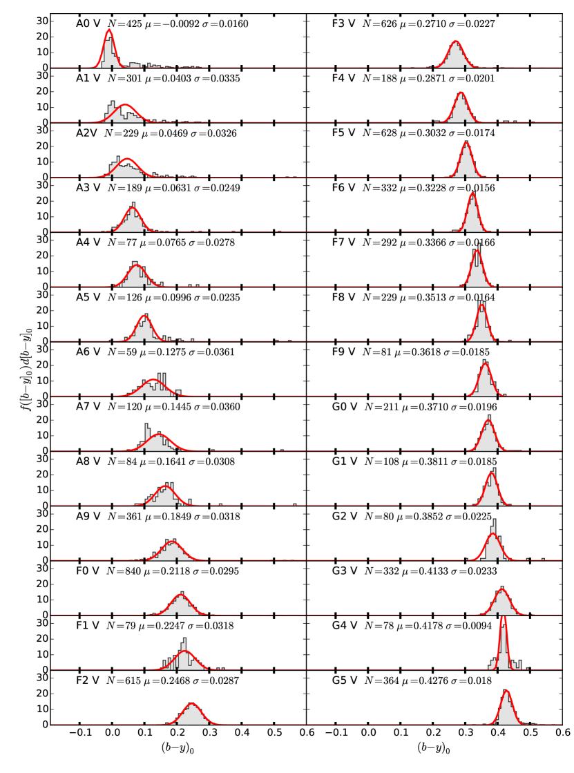
We generated the distributions of colors and color indices by spectral type for the 7054 main sequence stars from A0 to G5 of the sample. In Figure 4 we show the sequence of the index separated by spectral type.
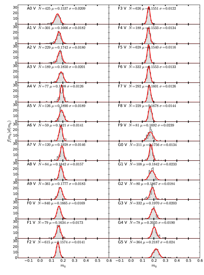
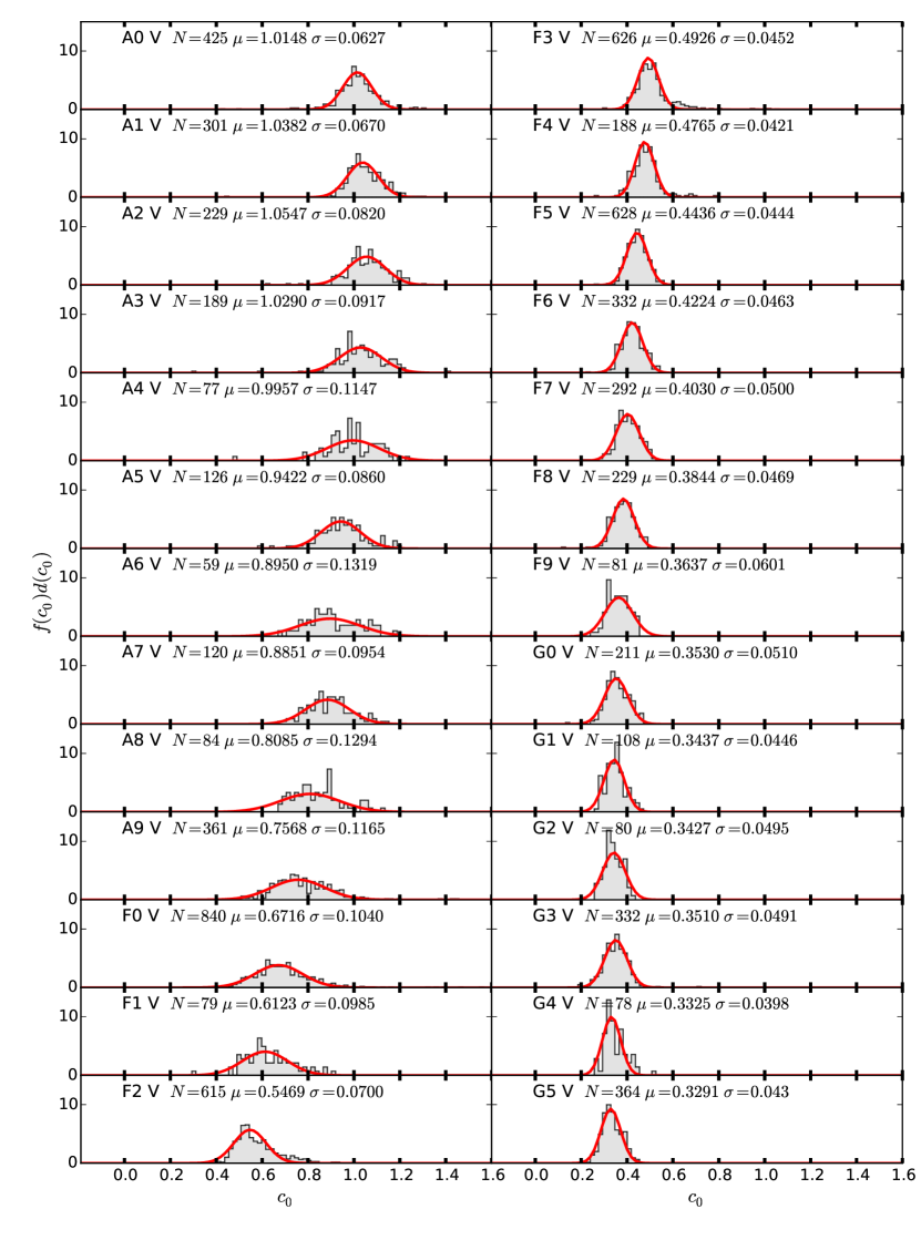
From the Central Limit Theorem, considering that we are comparing independent measurements (realizations) subject to variety of errors, we would expect the values of the indices per spectral type should follow a Normal distribution. We observed that highly discordant values occupied the tails of the distribution, while most of measurements cluster around their, respective, mean values. Indeed, from a Shapiro-Wilk test applied to the individual distributions, we obtained mean values of the test of , , and , for the indices , and , respectively. Although, the significance for the global distribution was low in certain cases; restricting the analysis around the mode yielded the non-rejection of the hypothesis of normality. Therefore, we suggest that the indices by spectral type are normally distributed. Therefore, we used Gaussian fits to model the distribution of indices by spectral type (red solid line). The distributions of and indices of our sample are shown in Figures 5 and 6, respectively.
Figure 4 shows a clear progression of the modes for each spectral type as a function of . This progression also confirms the one-to-one correspondence between stellar spectral type and effective temperature for main sequence stars (see §4). If we assign spectral types based on Strömgren photometry, our uncertainty is 2 types. This is due to the broadness of the color distribution. This is comparable to the results of Smriglio et al. (1990), who used the seven-filter Vilnius photometric system.
As seen in Figure 5, the metallicity index doesn’t follow any overall sequential pattern with spectral type. This fact could be explained by the selection itself, for we have included only non-peculiar stars within the solar-neighbourhood. Nevertheless, a slight progression is seen for stars later than F9, but its significance is weak with respect to the average for all the stars considered in this paper, which closely corresponds to the mean for G2 V stars.
On the other hand, a progression of the indicator of the Balmer Jump is clearly seen in Figure 6, but for spectral types later than A2 V and earlier than G0 V. However, has been known to be sensitive to the effective temperature of OB type stars, see also Fig. 8.
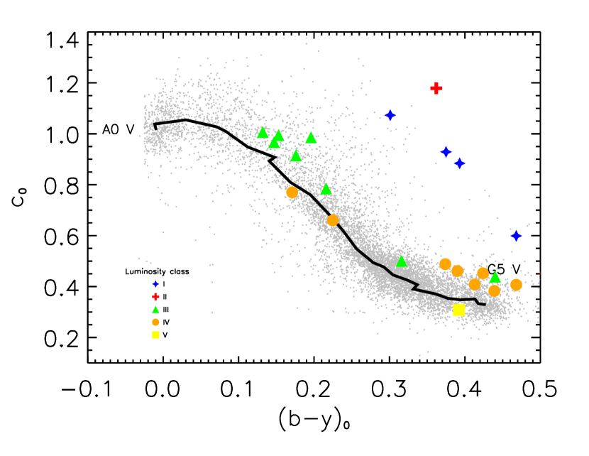
In Figure 7 we can see the locus of A0-G5 dwarfs in the - plane, first proposed by Strömgren (1966). Stars from Table 1 are shown in the plot using blue stars for luminosity class I, red crosses for II, green triangles for III, orange filled circles for IV, and yellow filled squares for V. These stars are MK standards taken from Table 1, the photometry was taken from Paunzen (2015) or SIMBAD, the distances from HIPPARCOS, and as explained in §2.1, no reddening correction was necessary (d 70 pc), and MV was obtained from the photometry provided by SIMBAD. These are consistent MK standards covering all luminosity classes. They were used to show their correspondence with surface gravity. The black thick line, depicts the locus of the mean and indices for each spectral type (Figures 5 and 6). Luminosity class V stars are concentrated in the grey band, and the position along this band determines the spectral class unambiguously. Supergiant stars are well separated from dwarf stars. Separation between class II and class I does not exist everywhere, but class II stars are also segregated from the main-sequence. Lastly, class III is not well distinguished from class IV and class V (cf., Gray, Napier, & Winkler, 2001). In Figure 7, we can appreciate that the original definition of the Strömgren photometric system did not include stars later than G5, as the separation between main sequence and evolve stars blurs for later types.
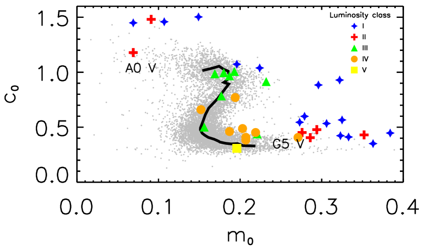
Figure 8 shows the distribution of the stars in the - plane (upper panel). The unreddened index, indicates the effective temperature; the index, the Balmer jump, i.e. the surface gravity and temperature. Note that the index comes to a maximum near , corresponding to the early A stars, where the Balmer lines and Balmer discontinuity reach their maximum excitation. The lower panel of Figure 8 shows the variation of with ; coloured symbols stand for the same as in Figure 7. There is a slight variation of about the solar metallicity.
4 Modelling of Physical Parameters
We used CHORIZOS: CHi-square cOde for parameterRized modeling and characterIZation of phOtometry and Spectrophotmetry (Maíz-Apellániz, 2004) to obtain the effective temperature () and surface gravity (). This code compares photometric data of a star with spectral energy distributions (SED) of model stellar atmospheres. The code calculates the likelihood for the full specified parameter ranges (interstellar extinction, , , metallicity), thus allowing for the identification of multiple solutions and the evaluation of the full correlation matrix for the derived parameters of a single solution.
In order to obtain the physical parameters, and correspondent for each spectral type from A0 to G0 V, we should find the SED that better fit our photometric data. For this aim, we used Strömgren color indices for each spectral type (e.g. Figure 4 for the mean ) with their respective uncertainties (the probable error derived from the fit to the color distribution by spectral type) as input parameters which are the mean , and and; a family of SED of Lejeune et al. (1997, 1998) with the following ranges: , .
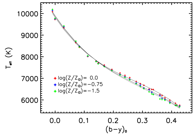
The range of metallicity considered by the code is , hence we tested for three different metallicities, from solar to subsolar. Figure 10 shows the effects of metallicity are mildly noticeable for stars later then F0 V. However, given the magnitude limit of mag, we find that all the the stars included in this study are closer than 950 pc; hence, they all belong to the solar neighbourhood. Therefore, fixing the metallicity to solar is justified. Besides, our choice is supported by the lack of strong variations of for the spectral types consider in this study, see Figure 5. Hence, for each spectral type the corresponding effective temperature and were obtained while keeping , fixed.
The fourth parameter we varied is the colour excess with the following range: , and the mean total to selective extinction ratio for the interstellar medium . As we already have a reddening-free sample of stars, therefore we fixed in CHORIZOS. We also conducted test considering the extinction as free parameter, this resulted in inconsistent outcomes.
We have tested both Kurucz (2004) and Lejeune et al. (1997, 1998) libraries for this study. In the results we obtain a discrepancy of a few hundreds of Kelvins in the effective temperature, we then have compared with fundamental temperatures of stars (see §4.1). The temperatures derived using Lejeune et al. libraries are closer to the fundamental temperatures; this transformation is consistent with the one suggested by David & Hillenbrand (2015). Therefore we adopted the Lejeune et al. libraries for the rest of this paper.
The effects of rotation have been ignored in the modeling described above. Nevertheless, the average rotational velocity decreases with spectral type (temperature), our sample covers stars from A0 to G5 type stars. Early type stars are early rotators, with rotational velocities of being typical. For a rotating star, both surface gravity and effective temperature decrease from the poles to the equator, changing the mean gravity and temperature of a rapid rotator relative to a slower rotator. The rotation of a star changes the width of a line in stellar spectra, hence resulting on a different classification.
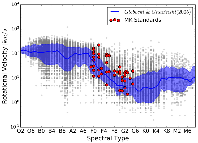
In Figure 9 we show a plot of the rotational velocities taken from Glebocki & Gnacinski (2005) (gray circles) for each spectral type where the blue curve is the median equatorial velocity, also in red circles are the velocity for MK standard stars listed in Table 1. The locus of the rotational velocity for the MK standard stars is in the same distribution for normal stars given the spectral type. Hence, in this work we have used stars whose spectra have been classified against normally rotation standard stars. This allowed us to exclude rapid rotators, at least statiscally. Moreover, slow rotators have been excluded to a first order by rejecting peculiar A stars (see §2).
Figueras & Blasi (1998), used Monte-Carlo simulations to investigate the effect of rapid rotation on the measured indices, derived parameters, and hence, isochronal ages of early-type star. Those authors concluded that excluding the effects of stellar rotation overestimates isochronal ages derived through photometric methods by 30/50 % on average.
Gray, Napier, & Winkler (2001) and Gray, Graham, & Hoyt (2001) suggested that stellar rotation and microturbulence velocity produces discrepancies between spectroscopic luminosity class and photometric indices. Some egregious discrepancies have been known among stars classified as dwarfs whose indices correspond to giant stars and vice versa. For example, And was classified F5 IV/V, but its measured index corresponds to a giant star (Gray, Napier, & Winkler, 2001).
Therefore, we have tried to compensate the effects produced by not including stellar rotation by considering the observed average properties of stars whose spectral properties resemble those of the MK standard stars in Table 1.
4.1 Correction by Confronting with Fundamental Parameters
Interferometric measurements of the stellar angular diameters and parallax measurements, allows the direct determination of effective temperature and the total integrated flux from a star. David & Hillenbrand (2015) compiled parameters derived through interferometric radii of 69 stars (listed in their table 1) whose values were taken from Boyajian et al. (2013) and Napiwotzki et al. (1993). Hence, using the photometry of main sequence stars, we have derived and using CHORIZOS, using the same input setup as in §4.
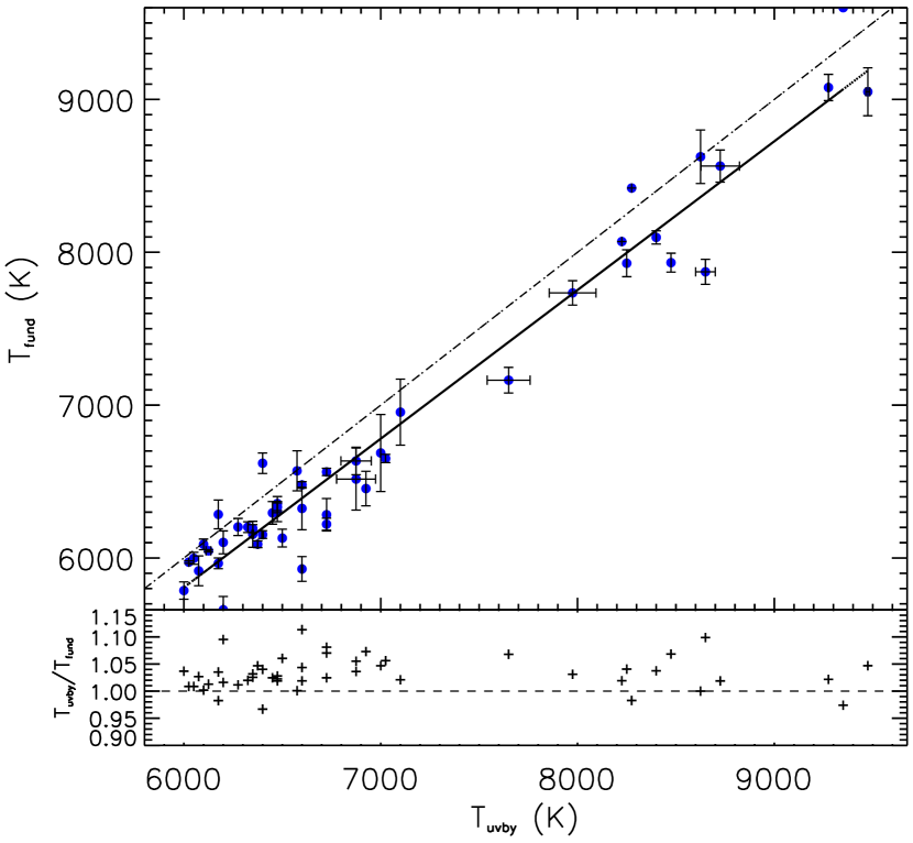
In Figure 11 we show a comparison of effective temperatures as provided by CHORIZOS with the compilation of fundamental effective temperatures of stars through interferometry listed in table 1 in David & Hillenbrand (2015). We found that the models predict () hotter effective temperatures than the ones provided by fundamental methods (). The dashed line is a one-to-one relation, most of the values of are below the dashed line. As a result from this comparison, we performed a linear fit (solid line) to the data. This fit is used as a correction to match the effective temperatures derived using stellar atmospheres models to those derived using fundamental methods:
| (1) |
This corrections is only valid for A0-G5 main sequence stars. This is in agreement with the transformations introduced by David & Hillenbrand (2015). Hence, the effective temperatures provided by CHORIZOS were corrected using Equation 1. Hereafter, we will only consider the corrected .
The slight discrepancy seen in Figure 11 was reported in previous studies (e.g., Bertone et al., 2004). It might be the result of incompleteness of line lists, the geometry, or non-LTE effects not accounted in the stellar atmosphere models (e.g., Önehag, Gustafsson, Eriksson & Edvardsson, 2009).
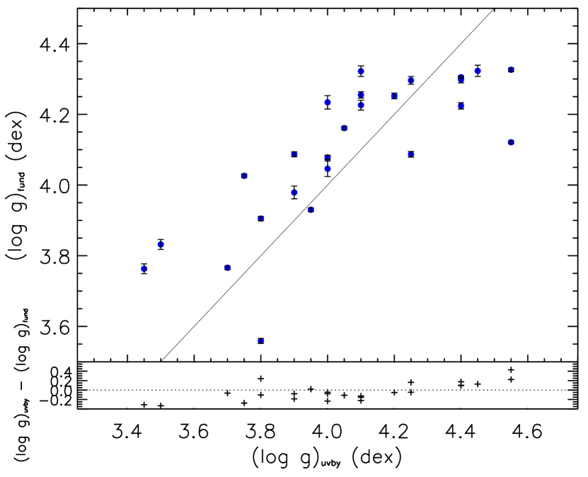
We have also compared the surface gravity , obtained with CHORIZOS with the corresponding stars values derived using fundamental methods (using eclipsing binarires) given in David & Hillenbrand (2015). In agreement with David & Hillenbrand, we only find a dispersion around the one-to-one relation, see Figure 12. Hence, we did not introduce any corrections to the derived surface gravity. Hereafter, we will refer to as .
Results
For each spectral type, from A0 V to G5 V (26 subclasses), we have derived and for two separated samples: stars closer than 70 pc (1496 stars) and the total sample which also includes derredened stars farther than 70 pc (7054 total), Tables 2 and 3, respectively. The errors in and were provided by CHORIZOS. There are slight differences for the parameters for each spectral class in these tables. As we discussed before, star earlier than A6 show a systematic shift when they are corrected assuming a regular extinction law (see Figure 3); this is expected, as young stars are embedded in the spiral arms. Later types (F and G) are distributed more isotropically, hence the effects of extinction are minimized. Nevertheless, the differences are within the errors.
We can see a clear progression for and which is shown in Figure 13 where a plot of versus the derived is shown for all the stars of our final sample. A third order linear polynomial accounts for temperature variations in the range between A0 V and G5 V stars, the resulting fit is:
| (2) |
The caveat in this calibration is that our statistical approach overlooks the effects of rotation, magnetic fields, metallicity variations, among others; besides, the models by Lejeune et al. (1997, 1998) are unidimensional and considered local thermal equilibrium (LTE). Nevertheless, we have found a tight correlation between spectral types, , and . Equation 4 is in agreement with previous calibrations such as Alonso et al. (1996); Gray, Graham, & Hoyt (2001) and tables 6 and 7 in Clem et al. (2004).
| Spectral | H | H | |||||||||
|---|---|---|---|---|---|---|---|---|---|---|---|
| Type | (K) | ||||||||||
| A0 V | 0.0004 | 0.0140 | 0.1609 | 0.0256 | 1.0317 | 0.0646 | 2.8917 | 0.0262 | 9326 285 | 4.33 0.24 | 1.11 0.58 |
| A1 V | 0.0177 | 0.0205 | 0.1786 | 0.0140 | 1.0043 | 0.0431 | 2.8997 | 0.0152 | 8984 258 | 4.43 0.15 | 1.42 0.49 |
| A2 V | 0.0306 | 0.0261 | 0.1802 | 0.0222 | 1.0241 | 0.0333 | 2.8918 | 0.0183 | 8701 275 | 4.35 0.21 | 1.48 0.56 |
| A3 V | 0.0559 | 0.0186 | 0.1835 | 0.0150 | 1.0114 | 0.0837 | 2.8799 | 0.0189 | 8321 219 | 4.41 0.22 | 1.46 0.64 |
| A4 V | 0.0705 | 0.0131 | 0.1928 | 0.0119 | 0.9432 | 0.0739 | 2.8559 | 0.0277 | 8232 89 | 4.49 0.05 | 1.89 0.45 |
| A5 V | 0.0957 | 0.0301 | 0.1919 | 0.0162 | 0.9514 | 0.0331 | 2.8452 | 0.0268 | 7979 276 | 4.58 0.31 | 1.79 0.51 |
| A7 V | 0.1136 | 0.0116 | 0.1997 | 0.0147 | 0.9054 | 0.0351 | 2.8286 | 0.0206 | 7513 36 | 4.01 0.10 | 1.86 0.55 |
| A8 V | 0.1502 | 0.0115 | 0.1825 | 0.0081 | 0.8326 | 0.0856 | 2.7835 | 0.0320 | 7505 52 | 4.17 0.26 | 1.96 0.63 |
| A9 V | 0.1781 | 0.0488 | 0.1717 | 0.0148 | 0.7605 | 0.1067 | 2.7525 | 0.0426 | 7201 375 | 4.72 0.31 | 2.49 0.54 |
| F0 V | 0.1980 | 0.0387 | 0.1690 | 0.0236 | 0.7133 | 0.1048 | 2.7428 | 0.0397 | 6987 230 | 4.52 0.39 | 2.55 0.50 |
| F1 V | 0.2221 | 0.0552 | 0.1619 | 0.0121 | 0.6144 | 0.0897 | 2.7266 | 0.0220 | 6922 277 | 4.60 0.35 | 2.90 0.30 |
| F2 V | 0.2551 | 0.0340 | 0.1531 | 0.0137 | 0.5412 | 0.0793 | 2.6944 | 0.0298 | 6712 143 | 4.54 0.35 | 3.02 0.41 |
| F3 V | 0.2715 | 0.0147 | 0.1492 | 0.0112 | 0.4800 | 0.0385 | 2.6708 | 0.0187 | 6566 82 | 4.43 0.25 | 3.27 0.37 |
| F4 V | 0.2899 | 0.0218 | 0.1563 | 0.0252 | 0.4644 | 0.0466 | 2.6625 | 0.0274 | 6419 128 | 4.52 0.34 | 3.13 0.55 |
| F5 V | 0.2988 | 0.0153 | 0.1538 | 0.0103 | 0.4324 | 0.0431 | 2.6518 | 0.0194 | 6341 100 | 4.42 0.32 | 3.44 0.47 |
| F6 V | 0.3196 | 0.0166 | 0.1546 | 0.0123 | 0.4149 | 0.0523 | 2.6397 | 0.0179 | 6285 45 | 4.47 0.31 | 3.50 0.52 |
| F7 V | 0.3345 | 0.0165 | 0.1587 | 0.0134 | 0.3881 | 0.0432 | 2.6280 | 0.0157 | 6078 80 | 4.42 0.34 | 3.64 0.55 |
| F8 V | 0.3499 | 0.0152 | 0.1678 | 0.0132 | 0.3755 | 0.0472 | 2.6195 | 0.0177 | 6047 30 | 4.42 0.34 | 3.87 0.52 |
| F9 V | 0.3600 | 0.0164 | 0.1687 | 0.0199 | 0.3477 | 0.0480 | 2.6053 | 0.0165 | 5887 118 | 4.53 0.35 | 4.08 0.62 |
| G0 V | 0.3733 | 0.0172 | 0.1757 | 0.0136 | 0.3429 | 0.0413 | 2.6045 | 0.0212 | 5808 19 | 4.42 0.37 | 4.20 0.61 |
| G1 V | 0.3832 | 0.0161 | 0.1862 | 0.0220 | 0.3417 | 0.0394 | 2.6066 | 0.0195 | 5804 28 | 4.47 0.39 | 4.14 0.61 |
| G2 V | 0.3927 | 0.0190 | 0.1901 | 0.0143 | 0.3302 | 0.0388 | 2.5977 | 0.0126 | 5744 110 | 4.48 0.38 | 4.37 0.49 |
| G3 V | 0.4042 | 0.0171 | 0.1979 | 0.0179 | 0.3336 | 0.0417 | 2.5936 | 0.0189 | 5565 23 | 4.45 0.39 | 4.55 0.55 |
| G4 V | 0.4130 | 0.0153 | 0.2099 | 0.0186 | 0.3284 | 0.0385 | 2.5881 | 0.0151 | 5563 21 | 4.42 0.41 | 4.51 0.48 |
| G5 V | 0.4253 | 0.0175 | 0.2220 | 0.0229 | 0.3168 | 0.0347 | 2.5897 | 0.0151 | 5562 19 | 4.44 0.44 | 4.89 0.49 |
| Spectral | H | H | |||||||||
|---|---|---|---|---|---|---|---|---|---|---|---|
| Type | (K) | ||||||||||
| A0 V | -0.0092 | 0.0108 | 0.1537 | 0.0209 | 1.0148 | 0.0627 | 2.8788 | 0.0341 | 9575 250 | 4.26 0.27 | |
| A1 V | 0.0403 | 0.0335 | 0.1666 | 0.0182 | 1.0382 | 0.0670 | 2.8841 | 0.0256 | 8792 468 | 4.46 0.32 | |
| A2 V | 0.0469 | 0.0326 | 0.1742 | 0.0180 | 1.0547 | 0.0820 | 2.8834 | 0.0265 | 8534 425 | 4.50 0.35 | |
| A3 V | 0.0631 | 0.0168 | 0.1850 | 0.0201 | 1.0290 | 0.0917 | 2.8693 | 0.0249 | 8217 247 | 4.40 0.27 | |
| A4 V | 0.0765 | 0.0278 | 0.1898 | 0.0126 | 0.9957 | 0.1147 | 2.8532 | 0.0302 | 8126 261 | 4.49 0.30 | |
| A5 V | 0.0996 | 0.0235 | 0.1890 | 0.0189 | 0.9422 | 0.0860 | 2.8310 | 0.0363 | 7892 213 | 4.46 0.26 | |
| A6 V | 0.1275 | 0.0538 | 0.1821 | 0.0141 | 0.8950 | 0.1319 | 2.8086 | 0.0392 | 7711 356 | 4.71 0.30 | |
| A7 V | 0.1445 | 0.0243 | 0.1928 | 0.0146 | 0.8851 | 0.0954 | 2.8078 | 0.0308 | 7382 320 | 4.54 0.37 | |
| A8 V | 0.1641 | 0.0308 | 0.1842 | 0.0157 | 0.8085 | 0.1294 | 2.7840 | 0.0365 | 7246 292 | 4.57 0.36 | |
| A9 V | 0.1849 | 0.0318 | 0.1777 | 0.0183 | 0.7568 | 0.1165 | 2.7578 | 0.0350 | 7032 226 | 4.48 0.42 | |
| F0 V | 0.2118 | 0.0295 | 0.1665 | 0.0169 | 0.6716 | 0.1040 | 2.7282 | 0.0325 | 6872 146 | 4.40 0.42 | |
| F1 V | 0.2247 | 0.0318 | 0.1634 | 0.0173 | 0.6123 | 0.0985 | 2.7168 | 0.0336 | 6832 138 | 4.49 0.39 | |
| F2 V | 0.2468 | 0.0287 | 0.1574 | 0.0141 | 0.5469 | 0.0700 | 2.6951 | 0.0266 | 6754 109 | 4.49 0.34 | |
| F3 V | 0.2710 | 0.0227 | 0.1551 | 0.0122 | 0.4926 | 0.0452 | 2.6739 | 0.0226 | 6596 115 | 4.46 0.29 | |
| F4 V | 0.2871 | 0.0201 | 0.1533 | 0.0134 | 0.4765 | 0.0421 | 2.6607 | 0.0207 | 6487 105 | 4.43 0.27 | |
| F5 V | 0.3032 | 0.0174 | 0.1540 | 0.0116 | 0.4436 | 0.0444 | 2.6507 | 0.0195 | 6310 64 | 4.35 0.33 | |
| F6 V | 0.3228 | 0.0156 | 0.1553 | 0.0133 | 0.4224 | 0.0463 | 2.6396 | 0.0171 | 6263 82 | 4.43 0.31 | |
| F7 V | 0.3366 | 0.0166 | 0.1601 | 0.0126 | 0.4030 | 0.0500 | 2.6291 | 0.0164 | 6061 52 | 4.33 0.37 | |
| F8 V | 0.3513 | 0.0164 | 0.1678 | 0.0144 | 0.3844 | 0.0469 | 2.6219 | 0.0170 | 6039 53 | 4.41 0.35 | |
| F9 V | 0.3618 | 0.0185 | 0.1692 | 0.0239 | 0.3637 | 0.0601 | 2.6102 | 0.0200 | 5859 103 | 4.55 0.37 | |
| G0 V | 0.3710 | 0.0196 | 0.1756 | 0.0134 | 0.3530 | 0.0510 | 2.6098 | 0.0211 | 5814 43 | 4.44 0.39 | |
| G1 V | 0.3811 | 0.0185 | 0.1842 | 0.0233 | 0.3437 | 0.0446 | 2.6071 | 0.0190 | 5804 29 | 4.52 0.38 | |
| G2 V | 0.3852 | 0.0225 | 0.1867 | 0.0184 | 0.3427 | 0.0495 | 2.5998 | 0.0168 | 5792 62 | 4.55 0.38 | |
| G3 V | 0.4133 | 0.0233 | 0.1970 | 0.0203 | 0.3510 | 0.0491 | 2.5941 | 0.0194 | 5565 23 | 4.49 0.42 | |
| G4 V | 0.4178 | 0.0094 | 0.2035 | 0.0190 | 0.3325 | 0.0398 | 2.5891 | 0.0156 | 5563 24 | 4.06 0.42 | |
| G5 V | 0.4276 | 0.0178 | 0.2187 | 0.0239 | 0.3291 | 0.0430 | 2.5896 | 0.0162 | 5560 28 | 4.40 0.46 |
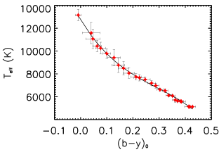
We also show the tight correspondence between and . For this aim we use the sample of stars within 70 pc (Table 2). Figure 14 that shows vs. . A second order polynomial can describe such correspondence:
| (3) |
From this we can also confirm that and vary with .
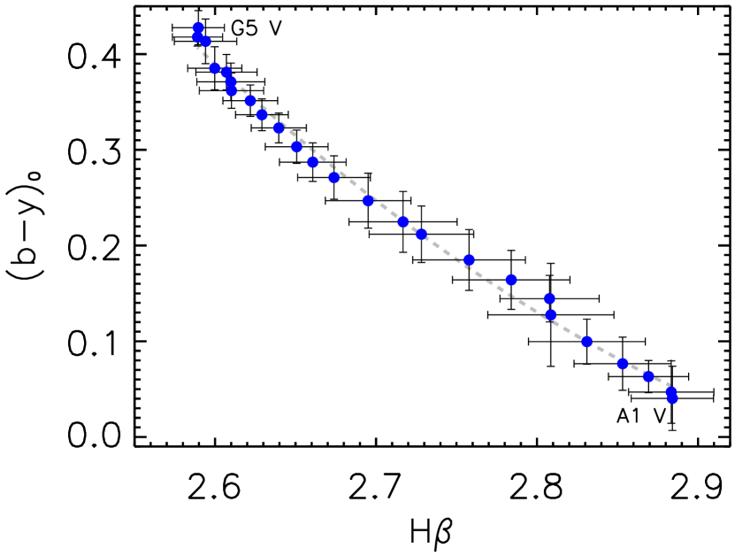
Table 2 is in close agreement with the results of Oblak et al. (1976); however, we have improved on the sampling of some spectral types and on the handle of interstellar reddening corrections. Tables 2 and 3 complement the calibrations presented in Apendix B of Gray & Corbally (2009). Hence, we suggest that the discrepancies in spectral types discussed in §2 are inconsequential to the main purpose of this work.
4.2 Comparison with Broad Band Photometric Systems
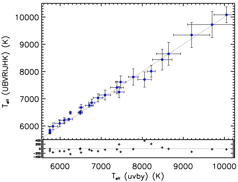
For a subsample of stars, we have consider broad band filters covering from the optical to the near infrared, we used UBVRIJHK photometry available in the literature. We run CHORIZOS for individual stars using UBVRIJHK and their respective Strömgren photometry.
We have compared the resulting effective temperatures in Figure 15 wih the . We can conclude from this, that broad band filters covering a much wider range than the Strömgren photometric system, provide only modest improvement in the determination of physical parameters. This result shows the effectiveness of the uvby- Strömgren-Crawford Photometric System over broad band photometry.
4.3 An Empirical Definition of Solar-Twin Candidates
A solar twin is a star with properties identical to the Sun. We can take the properties of the G2 V class in Table 3 to define the properties for solar-twin candidates (Garrison, 1979). The properties of solar-twin candidates are given in Table 4. Our definition agrees with the empirical definitions of Holmberg et al. (2006); Casagrande et al. (2010), but differs slightly with Meléndez et al. (2010) who defined a very narrow range of variation in the photometric properties. We should also remark that the physical properties of our solar-twin candidates agree with those of the Sun: K, , and (e.g., Gray, 2008). We can also add to Table 4 the value of the metaindex SM1 for G2 V stars, see §5, below.
We found 80 solar-twin candidates (cf., Ramírez et al., 2014). The 42 G2 V stars in Table 7 could also be considered as solar-twin candidates (§5.2.2). The study of the properties of solar twins is very important in the study of the evolution of the Sun and the formation of exoplanets.
The results presented in this section show that exploring the interplay among the MK system, an astrophysically motivated photometric system, and theory is very useful to broaden our insight on stellar structure, this was remarked earlier by Crawford (1984).
5 Automatic Classification Based on Strömgren Metaindices and Applications
We have recovered the physical basis of the MK spectroscopic classification. We can, then, search for alternative schemes for the classification and advance over the original scheme proposed by Strömgren. In this section, a principal component analysis (PCA) was applied to derive to established a new classification classification scheme. Our aim, is to derive a scheme that can be applied easily over a large spectroscopic range. Most of the reported photometry have been confined to , and ; hence, we limit our analysis to those parameters.
In Figure 16 we show the three-dimensional view of the average photometric color and indices for the complete sample of dwarf stars by MK spectral types in classical Strömgren color-indices space (squares). Standard stars from López-Cruz (1991) listed in Table 1; are shown in the plot using blue stars for luminosity class I, red crosses for II, green triangles for III, orange circles for IV and yellow squares for V. Dwarfs stars occupy a well-constrained subspace. The projections of this sequence are also shown in gray squares in the three planes. The details of the values of the dwarf sequence (black squares) are given in Table 3.

The Principal Component Analysis (PCA) is a statistical multivariate analysis method, proposed by Pearson (1901) to transform a set of possible correlated variables into a set of reduced uncorrelated variables. This method uses an orthogonal transformation to find a linear combination of its first variables with the condition to have the largest possible variance, this first linear combination is known as the first principal component (PC1). Then, the method finds a second linear combination that also has the largest variance with the additional condition to be orthogonal to the PC1, this second linear combination is known as the second principal component (PC2); and so on. Therefore we can represent the data into a new orthogonal space defined by the total number of principal components as their new axis; the maximum number of principal components is equal to the initial number of variables of the sample. One of the advantages of the PCA is that we can reduce the variable space into a new space of dimensions where is the number of principal components whose variances are less than the minimum variance of the data. This method is widely used in an astronomical context (e.g., Sheth & Bernardi, 2012; Steindling et al., 2001). Steindling et al. (2001) applied a PCA analysis to Strömgren photometric measurments of galaxies of different morphologies and nuclear activity. We follow Steindling et al. to form a better parametric description of our data.
5.1 From Strömgren colors to PCA Space: Definition of the “Dwarf-Star Box" and the “Supergiant Sequence"
We have a large sample of field stars for this study, all with intermediate band photometry. From a three-dimensional view of the color and the and indices we can see the position of the dwarf stars in a PCA space. We use the base vectors of this new coordinate system to define the following metaindices:
| (4) | |||||
| (5) | |||||
| (6) |
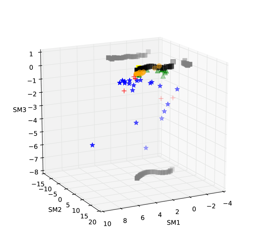
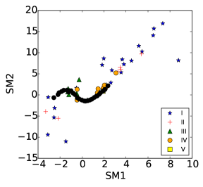
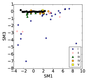
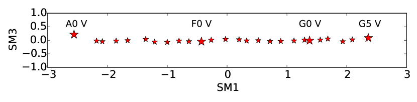
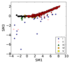
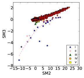
Figure 17 gives a view of the average photometric color and indices for the complete sample of dwarf stars by MK spectral types in Strömgren color-indexes (squares) projected onto a PCA space; the projections of this sequence are also shown in gray squares in the three planes, the projections of the planes are also shown in gray. Standard stars from López-Cruz (1991) with the same symbols as in Figure 7. In Figure 18 we see these projections, it clearly defines the sequence for dwarf stars in planes SM1-SM2 and SM1-SM3. From plane SM1-SM3 we determine that vector SM1 follows a clear separation between spectral types of the dwarf sequence from A0 V to G5 V stars. Lower values of SM1 correspond to early type stars while the higher ones correspond to late type stars. A zoom of this sequence is shown in Figure 19 where bigger symbols are only to guide the eye to the labels. It is evident that the spectral type is determined by the values of SM1 which are presented in Table 5. With the value of SM1 of any given star, we can assign a spectral type applying the nearest neighbour method. Hence, we can separate dwarfs from supergiants and bright giants and provide synthetic spectral types for A0V to G5 V stars.
| Spectral | SM1 | Spectral | SM1 | Spectral | SM1 |
|---|---|---|---|---|---|
| type | type | type | |||
| A0 V | -2.562 | F0 V | -0.430 | G0 V | 1.379 |
| A1 V | -2.183 | F1 V | -0.266 | G1 V | 1.558 |
| A2 V | -2.087 | F2 V | -0.026 | G2 V | 1.684 |
| A3 V | -1.856 | F3 V | 0.200 | G3 V | 1.935 |
| A4 V | -1.663 | F4 V | 0.327 | G4 V | 2.094 |
| A5 V | -1.362 | F5 V | 0.525 | G5 V | 2.361 |
| A6 V | -1.211 | F6 V | 0.718 | ||
| A7 V | -1.000 | F7 V | 0.897 | ||
| A8 V | -0.804 | F8 V | 1.119 | ||
| A9 V | -0.639 | F9 V | 1.295 |
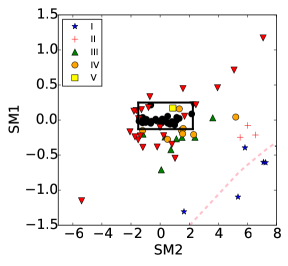
Panel the right panel defines a “Dwarf-Star box" where stars located within:
| (7) |
This box is partially contaminated by subdwarfs; however, none of the higher luminosity classes contaminate this box. Hence, stars falling in this box can be classified automatically as luminosity class V stars. We can also define the main sequence for A0-G5 stars, directly from SM3 (Equation 6):
| (8) |
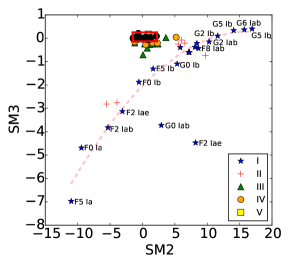
The pink dashed line in the SM3 vs. SM2 diagram (see Figure 18, lower panel) is a parametrization to the supergiant stars. A second order polynomial defined by:
| (9) |
provides an adequate fit, we call this the Supergiant Sequence. The progression doesn’t follow the distribution of spectral types as cleanly as the dwarfs. Supergiants with negative values of SM2 and SM3 are earlier than G2 I; however do not follow a clear progression with spectral type. Nevertheless, for types later than G2 the supergiants hint a progression with spectral type. Also, bright giants (II) seem to scattered around Equation 9. More work is needed to establish the metaindex distribution for supergiants and bright giants. We should also take into account the effects of microturbulence (Gray, Graham, & Hoyt, 2001; Gray & Corbally, 2009, pp. 226-227), winds and the intrinsic instabilities in the structure of supergiants. Nevertheless, the resulting transformations separate dwarfs from supergiants and bright giants into perpendicular planes; therefore, we can use this information to separate these three luminosity classes, unambiguously. We can also a attempt to segregate subgiants and giants, but there is no discernible trend related to the spectral type.
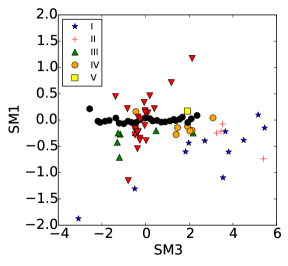
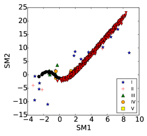
Summarizing the properties of the metaindices: the SM2 vs. SM1 plane provides nearly the same information as the vs. diagram (Fig. 7). The SM3 vs. SM1 plane provides the main sequence for A0-G5 stars, in this projection the main sequence can be described by straight line (Equation 8). The SM3 vs. SM2 plane provides the dwarf star box (Equation 7) and the sequence for supergiants and bright giants (Equation 9). A synthetic classification scheme can be implemented using the metaindices SM1, SM2, and SM3 as given by Equations 4, 5 and 6 respectively. All that is needed is a set unreddened Strömgren photometric measurements. Stars falling into the Dwarf Star Box are selected as main sequence stars. Then by interpolation using Equation 8, we can generated a spectral type. Supergiants and bright giants can be separated using Equation 9. Given the small contamination of the Dwarf Star Box, stars not falling on the supergiant sequence, and outside the Box could be considered giants or subgiants.
5.2 Applications of the New Classification Scheme
We present two applications of the metaindices formalism introduced above. We consider a sample of candidate F supergiants. Separetely, we also consider a set of high-velocity stars. Very few of those high-velocity stars had luminosity classes assigned before.
5.2.1 Search for Supergiants Stars in the Halo of our Galaxy
Arellano Ferro et al. (1989) generated a -H photometric study for a group candidates F-type supergiants at high galatic latitude. The spectral types were provided by Bartaya (1979) from objective prism plates. Arellano Ferro et al. concluded that most of the stars had solar abundances and gravities larger than 3.0, and suggested that most of these stars were low mass stars of the old disk population.
We can test Arellano Ferro et al. result straightforwardly. We have taken the four color observations presented in Table 4 from Arellano Ferro et al. (1989). The reddening for each of the candidates is given in column 2 of their Table 7. The stars were dereddened according to the following equations: ; ; (Crawford, 1975). The reddening corrections are small.
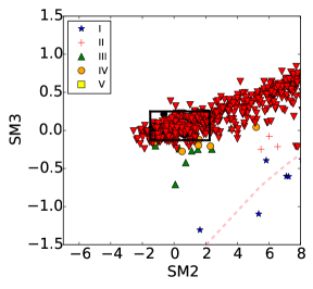
The metaindices were generated according to Equations 4, 5 and 6. Figure 20 shows the positions these stars in red downside triangles in two of our diagnostic diagrams. From SM2-SM3 plot we can find six stars falling inside the “Dwarf-Stars Box", while the rest of them, are distributed around the box, but away the parametrization for supergiants and bright giants. For the six dwarfs, we can provide stellar spectral classification by interpolation in Table 5, using the nearest neighbour method. The results are listed in Table 6. In column 3 is the classification proposed by Bartaya (1979), in column 4 is the classification reported by SIMBAD, in column 5 we provide the spectrla types assigned by following MK process strictly performed by López-Cruz (1991) and later reported by López-Cruz & Garrison (1993), in column 6 we provide types reported in the compilation by Skiff (2014), and finally in column 7 we present our new synthetical classifications. There is a general agreement with the published classifications, the uncertainty on the spectral type falls within the uncertainties (see §3). However, the most discrepant is the stars BD +45 1459 (HD 60653) classified as a giant (F5 III) by López-Cruz (1991) but with photometric indices corresponding to F2 V star; this star might represent another egregious discrepancy (Gray, Napier, & Winkler, 2001). The rest of the stars fall very close to the regions occupied by subdwarfs or giant stars. Moreover, stars on the upper right region outside the Dwarf-Star Box in the SM3 vs. SM2 diagram (Figure 20, lower panel), could be considered late type G or early K dwarfs (see §5.2.2); therefore, we can conclude that none of the stars included in the study of Arellano Ferro et al. (1989) are supergiants.
Our results show that the classifications provided by Bartaya (1979) were inaccurate, in agreement with the results of Arellano Ferro et al. (1989), López-Cruz (1991), and López-Cruz & Garrison (1993).
| BD/BSD | HD | SPECTRAL TYPE | ||||
|---|---|---|---|---|---|---|
| Bartaya (1979) | SIMBAD | López-Cruz & Garrison (1993) | Skiff (2014) | This work | ||
| +61 959 | 56664 | F0 I | F0 | - | - | A8 V |
| +45 1459 | 60653 | F3 I | F2 | F5 III | F2 III/IV | F2 V |
| +45 1462 | 60712 | F5 I | F2 | - | - | F2 V |
| +45 1507 | 64445 | F5 Ib | G0 | - | - | F2 V |
| +45 1624 | 74132 | F5 I | F5 | F2 V | - | F1 V |
| +45 1769 | 85039 | F5 I | F3 III | F3 IV | F3 Vn | F2 V |
SIMBAD does not report the reference of those six classifications.
5.2.2 Classification of High Velocity Stars with High Metallicity
From a sample of high-velocity stars studied by Schuster & Nissen (1988) and Schuster et al. (1993, 2006), we have selected 761 stars with metallicities close to the Sun (). These stars are distributed uniformly over the sky; that is, there are no significant north-south differences. There are F, G and early K-type stars are in the sample. We corrected for interstellar extinction when . Then, we have applied the metaindices transformation equations as in the previous example. Figure 21 depicts the distribution of the selected stars, while Figure 22 is a zoom around the Dwarf-Star box. There are 254 stars inside the box, we label them with the luminosity class V. We provide the synthetic spectral types for these stars in Tables 7 and 8, they are presented in the column SC. Table 9 summarize our results. Column named PC in Tables 7 and 8 present published classifications. We found 57 stars with full spectral classifications (spectral type and luminosity class). We evaluated the difference between the synthetic classification and the published classification, we found that the mean, the median, and the mode are zero, while the standard deviation is SD=2.95. Only the star G060-067 (HD 114174) has been spectroscopically classified as a subgiant, its published type is G5 IV (Roman, 1955); hence, we can say that the Dwarf-Star box has a contamination of about 2 %. We conclude that by using our classification scheme, based on metaindices, we can provide synthetic spectral classifications with an uncertainty of about 2 MK spectral types (see §3) and about 98 % precision in the luminosity class for dwarf stars. We are limited by the accuracy of the photometric measurements and the spread of the stellar physical properties for each MK spectral type (§3). Our sample of 254 classified high-velocity stars can be considered for further studies of the galactic structure (e.g., Silva et al., 2012) or exoplanet studies, as there are 45 solar-twin candidates in Table 7.
In the SM3-SM2 digram (Figure 21, lower panel) there are three stars near to the supergiant sequence, these stars could be considered supergiant candidates. Nevertheless, their reported classifications corresponds to late dwarf stars G014-032 (G8 V), G080-016 (K1 V) and G016-032 (K0 IV). Hence, we suggest that these stars should be considered in the egregious discrepancy category (Gray, Napier, & Winkler, 2001).
The long tail traced by red downside triangles with positive values for SM1, SM2, and SM3 outside the Dwarf-Star Box in Figures 21 and 22, are late type dwarfs: later than G5 V but earlier than K4 V. It seem that the separation among dwarfs and supergiants is also preserved, see Figures 21, 22. This looks very promising, as our formalism can be extended by generation a new set of metaindices to cover from A0 through K4 stars. This represents an economic extension of Stömgren Photometric System because it avoids the introduction of any new photometric filter (e.g., the filter, Anthony-Twarog et al., 1991). We will consider this option in a furture study.
| Star | V | H | PC | SC | Star | V | H | PC | SC | ||||||
|---|---|---|---|---|---|---|---|---|---|---|---|---|---|---|---|
| HD 82328 | 3.170 | 0.314 | 0.153 | 0.463 | 2.646 | F7V | F5 V | HD 94518 | 8.340 | 0.383 | 0.172 | 0.273 | 2.597 | G2 V | G2 V |
| LTT15703 | 8.514 | 0.305 | 0.159 | 0.474 | 2.666 | F6 | F5 V | HD 49409 | 7.922 | 0.385 | 0.176 | 0.298 | 2.580 | G2 | G2 V |
| G114-025 | 10.654 | 0.296 | 0.155 | 0.422 | 2.626 | F7 V | F5V | G127-048 | 8.670 | 0.380 | 0.189 | 0.356 | 2.603 | G5 | G2 V |
| HD 298812 | 9.292 | 0.332 | 0.153 | 0.443 | 0.000 | F8 | F6 V | HD 97507 | 8.590 | 0.392 | 0.176 | 0.307 | 2.571 | G3 V | G2 V |
| HD 143333 | 5.457 | 0.333 | 0.154 | 0.448 | 2.620 | F8 V | F6 V | HD 143464 | 10.008 | 0.402 | 0.176 | 0.327 | 2.573 | G5 (V) | G2 V |
| HD 82152 | 8.109 | 0.323 | 0.159 | 0.415 | 0.000 | F7 V | F6 V | HD 87998 | 7.265 | 0.391 | 0.181 | 0.328 | 2.610 | G0 V | G2 V |
| HD 98220 | 6.848 | 0.328 | 0.158 | 0.382 | 2.635 | F7 V | F7 V | LTT15705 | 8.060 | 0.410 | 0.175 | 0.335 | 2.581 | F8 | G2 V |
| LTT15336 | 6.804 | 0.336 | 0.163 | 0.412 | 2.631 | F5 V | F7 V | HD 20807 | 5.232 | 0.383 | 0.179 | 0.299 | 2.602 | G1 V | G2 V |
| HD 20052 | 10.151 | 0.356 | 0.153 | 0.359 | 2.603 | F8V | F8 V | HD 6517 | 8.959 | 0.402 | 0.178 | 0.333 | 2.574 | G0 V | G2 V |
| LTT15268 | 8.525 | 0.349 | 0.158 | 0.340 | 2.619 | F8 | F8 V | G027-022 | 8.895 | 0.382 | 0.193 | 0.371 | 2.614 | G2-3 V | G2 V |
| LTT16139 | 6.573 | 0.364 | 0.162 | 0.379 | 2.618 | F8 | F8 V | HD 24049 | 9.480 | 0.390 | 0.173 | 0.278 | 2.566 | G3 V | G2 V |
| G061-014 | 6.832 | 0.348 | 0.170 | 0.378 | 2.621 | F8 V | F8 V | G067-049 | 8.559 | 0.385 | 0.186 | 0.336 | 2.601 | G5 | G2 V |
| HD 31460 | 8.047 | 0.376 | 0.156 | 0.354 | 2.588 | G0V | F8 V | HD 90197 | 7.055 | 0.408 | 0.173 | 0.313 | 2.575 | G3/G5 V | G2 V |
| HD 120237 | 6.584 | 0.355 | 0.167 | 0.364 | 2.642 | G0 V | F8 V | G026-020 | 8.910 | 0.392 | 0.173 | 0.278 | 2.571 | G0 V | G2 V |
| G043-033 | 7.887 | 0.365 | 0.159 | 0.311 | 2.585 | Gwl | F9 V | G102-042 | 8.180 | 0.407 | 0.177 | 0.329 | 2.585 | G0 | G2 V |
| HD 4156 | 9.347 | 0.381 | 0.157 | 0.312 | 2.585 | G3 V | F9 V | G091-020 | 7.301 | 0.393 | 0.190 | 0.369 | 2.603 | G0 | G2 V |
| HD 203448 | 7.821 | 0.375 | 0.175 | 0.392 | 2.606 | G1/2 V | F9 V | HD 3628 | 7.347 | 0.406 | 0.182 | 0.350 | 2.592 | G3 V | G2 V |
| G171-064 | 7.387 | 0.350 | 0.177 | 0.348 | 2.613 | F8 | F9 V | G034-016 | 8.441 | 0.397 | 0.182 | 0.331 | 2.598 | G5 | G2 V |
| HD 32023 | 9.174 | 0.341 | 0.182 | 0.355 | 2.586 | F7 V | F9 V | HD 100504 | 8.560 | 0.389 | 0.185 | 0.329 | 2.592 | G1 V | G2 V |
| HD 114729 | 6.687 | 0.391 | 0.163 | 0.344 | 0.000 | G0 V | G0 V | HD 190649 | 8.837 | 0.415 | 0.173 | 0.318 | 2.566 | G5 V | G2 V |
| HD 43745 | 6.062 | 0.355 | 0.192 | 0.418 | 2.614 | F8.5 V | G0 V | G034-036 | 9.043 | 0.405 | 0.172 | 0.289 | 2.578 | G5 | G2 V |
| G099-040 | 9.202 | 0.376 | 0.162 | 0.298 | 2.582 | F8 | G0 V | HD 178496 | 8.172 | 0.405 | 0.182 | 0.343 | 2.573 | G3 V | G2 V |
| G105-038 | 7.615 | 0.387 | 0.167 | 0.347 | 2.595 | G0 | G0 V | HD 28571 | 8.982 | 0.405 | 0.183 | 0.346 | 2.584 | G5 V | G2 V |
| HD 30361 | 8.346 | 0.385 | 0.162 | 0.315 | 2.576 | G0 | G0 V | HD 196800 | 7.210 | 0.388 | 0.196 | 0.380 | 2.611 | G1-2 | G2 V |
| G114-B8A | 10.242 | 0.378 | 0.164 | 0.303 | 2.605 | dF8 | G0 V | G031-003 | 8.380 | 0.397 | 0.188 | 0.354 | 2.593 | G0 | G2 V |
| CD-31 8004 | 9.812 | 0.383 | 0.177 | 0.380 | 2.642 | G0 | G0 V | HD 237822 | 9.988 | 0.397 | 0.177 | 0.294 | 2.568 | G3 V | G2 V |
| G156-019 | 8.746 | 0.374 | 0.163 | 0.284 | 2.592 | G3 V | G0 V | G013-001 | 9.020 | 0.368 | 0.183 | 0.265 | 2.590 | G3 V | G2 V |
| HD 83529 | 6.971 | 0.377 | 0.171 | 0.325 | 2.602 | G3 V | G0 V | G095-004 | 8.621 | 0.410 | 0.176 | 0.313 | 2.592 | G0 | G2 V |
| G219-020 | 9.505 | 0.383 | 0.162 | 0.287 | 2.579 | G2 | G0 V | G065-016 | 8.556 | 0.399 | 0.179 | 0.301 | 2.580 | G2 | G2 V |
| HD 157214 | 5.384 | 0.400 | 0.163 | 0.327 | 2.572 | G0 V | G0 V | HD 25535 | 6.738 | 0.393 | 0.190 | 0.347 | 2.598 | G1-2 V | G2 V |
| HD 212231 | 7.874 | 0.398 | 0.165 | 0.333 | 2.579 | G2 V | G0 V | HD 184700 | 8.837 | 0.416 | 0.182 | 0.351 | 2.581 | G3 V | G2 V |
| G089-034 | 8.197 | 0.398 | 0.163 | 0.322 | 2.578 | G0 | G0 V | HD 10785 | 8.520 | 0.381 | 0.192 | 0.326 | 2.593 | G1-2 V | G2 V |
| G103-031 | 10.253 | 0.384 | 0.162 | 0.287 | 2.580 | G0 | G0 V | HD 98966 | 9.356 | 0.421 | 0.180 | 0.342 | 2.635 | G3wF7V | G2 V |
| HD 132996 | 7.773 | 0.393 | 0.170 | 0.349 | 2.604 | G3 V | G0 V | G066-035 | 8.725 | 0.402 | 0.189 | 0.349 | 2.594 | G3 V | G2 V |
| G188-029 | 9.144 | 0.379 | 0.181 | 0.378 | 2.624 | G0 | G0 V | G130-029 | 7.841 | 0.407 | 0.198 | 0.408 | 2.608 | G0 | G2 V |
| HD 102158 | 8.066 | 0.393 | 0.163 | 0.309 | 2.581 | G2 | G1 V | HD 185203 | 9.012 | 0.416 | 0.183 | 0.345 | 2.581 | G5 V | G2 V |
| HD 111564 | 7.615 | 0.381 | 0.181 | 0.381 | 2.620 | G0 V | G1 V | HD 156802 | 7.939 | 0.416 | 0.180 | 0.328 | 2.574 | G2 V | G2 V |
| G126-059 | 7.571 | 0.389 | 0.174 | 0.351 | 2.597 | G4 | G1 V | G063-051 | 6.925 | 0.411 | 0.193 | 0.387 | 2.588 | G2 V | G2 V |
| G001-051 | 7.224 | 0.375 | 0.178 | 0.343 | 2.602 | G0 | G1 V | HD 115031 | 8.334 | 0.395 | 0.192 | 0.348 | 2.602 | G2-3 V | G2 V |
| G162-016 | 9.799 | 0.396 | 0.167 | 0.323 | 2.586 | G5 V | G1 V | G029-065 | 7.690 | 0.400 | 0.193 | 0.358 | 2.598 | G5 V | G2 V |
| HD 165401 | 6.804 | 0.392 | 0.163 | 0.293 | 2.580 | G2 V | G1 V | HD 165271 | 7.646 | 0.416 | 0.196 | 0.407 | 2.592 | G5 V | G2 V |
| HD 149996 | 8.495 | 0.396 | 0.164 | 0.305 | 2.572 | G1 V | G1 V | G099-050 | 10.227 | 0.387 | 0.182 | 0.267 | 2.560 | F2 | G2 V |
| G097-025 | 7.008 | 0.375 | 0.176 | 0.324 | 2.595 | G0 V | G1 V | HD 88371 | 8.414 | 0.407 | 0.186 | 0.329 | 2.584 | G2 V | G2 V |
| LFT1036 | 6.335 | 0.401 | 0.182 | 0.409 | 2.597 | G0 V | G1 V | G134-003 | 10.321 | 0.406 | 0.177 | 0.278 | 2.582 | G6 | G2 V |
| HD 62549 | 7.723 | 0.385 | 0.182 | 0.375 | 2.605 | G2-3 V | G1 V | HD 53705 | 5.557 | 0.383 | 0.194 | 0.319 | 2.595 | G1.5 V | G3 V |
| HD 101614 | 6.861 | 0.377 | 0.168 | 0.282 | 2.602 | G0 V | G1 V | HD 56196 | 8.944 | 0.388 | 0.198 | 0.350 | 2.595 | G5 | G3 V |
| G071-027 | 8.898 | 0.347 | 0.177 | 0.266 | 2.590 | G0 IV-V | G1 V | G071-040 | 7.426 | 0.400 | 0.189 | 0.326 | 2.582 | G5 V | G3 V |
| G192-023 | 7.470 | 0.377 | 0.183 | 0.357 | 2.599 | G0 | G1 V | G005-044 | 9.170 | 0.403 | 0.190 | 0.337 | 2.594 | G0 | G3 V |
| HD 158630 | 7.609 | 0.381 | 0.174 | 0.312 | 2.600 | G0 V | G1 V | HD 68978 | 6.719 | 0.373 | 0.203 | 0.342 | 0.000 | G0.5 V | G3 V |
| HD 2070 | 6.818 | 0.375 | 0.185 | 0.358 | 2.602 | G0 V | G1 V | G065-047 | 6.270 | 0.410 | 0.178 | 0.284 | 2.574 | G1.5 V | G3 V |
| HD 98868 | 9.640 | 0.375 | 0.176 | 0.304 | 2.611 | G3 V | G1 V | HD 199190 | 6.872 | 0.397 | 0.202 | 0.383 | 2.607 | G1 IV-V | G3 V |
| G060-031 | 9.517 | 0.387 | 0.170 | 0.294 | 2.586 | G3V | G1 V | HD 110313 | 7.886 | 0.386 | 0.201 | 0.354 | 2.612 | F8 | G3 V |
| HD 211476 | 7.046 | 0.389 | 0.175 | 0.325 | 2.599 | G2 | G1 V | G132-073 | 7.832 | 0.397 | 0.198 | 0.360 | 2.604 | G0 | G3 V |
| G093-047 | 10.700 | 0.396 | 0.172 | 0.322 | 2.586 | G5 | G1 V | G054-021 | 7.583 | 0.386 | 0.194 | 0.313 | 2.602 | G0 V | G3 V |
| G033-048 | 8.754 | 0.388 | 0.169 | 0.289 | 2.586 | G0 | G1 V | HD 18605 | 9.566 | 0.405 | 0.181 | 0.282 | 2.573 | G6-8 V | G3 V |
| HD 167425 | 6.192 | 0.376 | 0.187 | 0.359 | 2.614 | F9.5 V | G1 V | HD 118475 | 6.976 | 0.386 | 0.206 | 0.372 | 2.630 | F9VFe+0.3 | G3 V |
| G014-026 | 9.732 | 0.387 | 0.181 | 0.349 | 2.590 | G1 V | G1 V | HD 3074 | 6.414 | 0.382 | 0.206 | 0.363 | 2.616 | F8-G0V | G3 V |
| HD 198188 | 8.129 | 0.385 | 0.181 | 0.340 | 2.599 | G3 V | G1 V | G101-041 | 7.135 | 0.396 | 0.181 | 0.257 | 2.565 | G1 V | G3 V |
| G054-007 | 7.782 | 0.375 | 0.180 | 0.313 | 2.593 | G0 | G1 V | G018-005 | 9.262 | 0.401 | 0.183 | 0.276 | 2.579 | G3 V | G3 V |
| HD 162756 | 7.642 | 0.392 | 0.182 | 0.358 | 2.587 | F8-G0V | G1 V | HD 11828 | 9.280 | 0.406 | 0.188 | 0.310 | 2.575 | G5 V | G3 V |
| G103-058 | 10.018 | 0.395 | 0.170 | 0.299 | 2.594 | sd?G2 | G1 V | G131-053 | 9.376 | 0.395 | 0.203 | 0.368 | 2.606 | G0 | G3 V |
| G018-035 | 8.448 | 0.388 | 0.173 | 0.298 | 2.587 | G0 | G1 V | G059-025 | 8.736 | 0.388 | 0.196 | 0.315 | 2.593 | G3 V | G3 V |
| HD 78558 | 7.297 | 0.391 | 0.174 | 0.307 | 2.585 | G0.5 V | G1 V | G066-033 | 9.528 | 0.399 | 0.190 | 0.304 | 2.584 | F8 | G3 V |
| G085-045 | 8.451 | 0.385 | 0.187 | 0.359 | 2.601 | G5 | G2 V | G073-051 | 8.837 | 0.398 | 0.188 | 0.290 | 2.583 | G5 | G3 V |
| ID | V | H | PC | SC | ID | V | H | PC | SC | ||||||
|---|---|---|---|---|---|---|---|---|---|---|---|---|---|---|---|
| HD 60298 | 7.373 | 0.401 | 0.197 | 0.340 | 2.586 | – | G3 V | G087-002 | 8.816 | 0.417 | 0.208 | 0.298 | 2.584 | G0 | G5 V |
| HD 89832 | 9.036 | 0.410 | 0.186 | 0.296 | 2.576 | G3-5 V | G3 V | HD 22380 | 8.636 | 0.414 | 0.217 | 0.339 | 2.584 | G5 V | G5 V |
| HD 61986 | 8.684 | 0.390 | 0.191 | 0.279 | 0.000 | G5 V | G3 V | HD 108309 | 6.246 | 0.422 | 0.220 | 0.371 | 2.609 | G2V | G5 V |
| HD 184704 | 9.337 | 0.410 | 0.204 | 0.391 | 2.599 | G0-2 V | G3 V | G062-023 | 8.423 | 0.420 | 0.213 | 0.328 | 2.583 | G9 | G5 V |
| HD 97998 | 7.362 | 0.397 | 0.185 | 0.260 | 2.599 | G1 V | G3 V | G092-016 | 10.178 | 0.441 | 0.199 | 0.296 | 2.565 | G0 | G5 V |
| G018-060 | 8.188 | 0.415 | 0.192 | 0.334 | 2.579 | G6V | G3 V | G114-048 | 10.649 | 0.409 | 0.213 | 0.304 | 2.586 | – | G5 V |
| HD 4308 | 6.552 | 0.408 | 0.190 | 0.307 | 2.578 | G6 VFe-0.9 | G3 V | HD 123682 | 8.312 | 0.416 | 0.212 | 0.313 | 0.000 | G3-5 V | G5 V |
| G069-008 | 9.015 | 0.404 | 0.186 | 0.275 | 2.586 | G0 | G3 V | G127-012 | 8.938 | 0.415 | 0.219 | 0.347 | 2.595 | G0 | G5 V |
| HD 189567 | 6.080 | 0.407 | 0.190 | 0.302 | 2.583 | G2 V | G3 V | G030-034 | 9.168 | 0.423 | 0.201 | 0.265 | 2.551 | G6 | G5 V |
| G131-059 | 7.573 | 0.408 | 0.198 | 0.345 | 2.594 | F8 | G3 V | G023-006 | 7.918 | 0.418 | 0.217 | 0.340 | 2.586 | G5 | G5 V |
| HD 223171 | 6.888 | 0.414 | 0.203 | 0.382 | 2.598 | G2 V | G3 V | HD 4096 | 9.242 | 0.418 | 0.215 | 0.326 | 2.582 | G3 V | G5 V |
| HD 224383 | 7.896 | 0.403 | 0.200 | 0.341 | 2.593 | G3 V | G3 V | G044-044 | 8.160 | 0.407 | 0.218 | 0.319 | 2.579 | G2 | G5 V |
| HD 30562 | 5.770 | 0.395 | 0.216 | 0.409 | 2.615 | G2 IV | G3 V | HD 184768 | 7.557 | 0.427 | 0.216 | 0.348 | 2.587 | G5 V | G5 V |
| G061-030 | 8.493 | 0.388 | 0.203 | 0.323 | 2.596 | G0 | G3 V | G126-012 | 8.614 | 0.428 | 0.219 | 0.365 | 2.590 | G5 | G5 V |
| HD 65243 | 8.013 | 0.388 | 0.202 | 0.317 | 0.000 | G3-5 V | G3 V | G078-041 | 10.231 | 0.419 | 0.205 | 0.270 | 2.561 | G0 | G5 V |
| G082-012 | 7.880 | 0.408 | 0.197 | 0.329 | 2.581 | G3 V | G3 V | G028-035 | 9.244 | 0.413 | 0.209 | 0.278 | 2.574 | G6 V | G5 V |
| HD 189931 | 6.911 | 0.395 | 0.202 | 0.328 | 2.596 | G1 V | G3 V | HD 110619 | 7.530 | 0.413 | 0.205 | 0.256 | 2.580 | G5 V | G5 V |
| HD 174995 | 8.494 | 0.410 | 0.193 | 0.310 | 2.578 | G9 | G3 V | CD-26 3087 | 9.759 | 0.438 | 0.204 | 0.302 | 2.538 | G8 | G5 V |
| G058-030 | 7.933 | 0.388 | 0.211 | 0.356 | 2.610 | G0 | G3 V | G013-054 | 7.841 | 0.424 | 0.226 | 0.391 | 2.592 | G6-8 V | G5 V |
| G088-008 | 7.995 | 0.394 | 0.201 | 0.312 | 2.599 | G4 | G3 V | G034-003 | 7.619 | 0.424 | 0.211 | 0.309 | 2.575 | G5 | G5 V |
| G092-015 | 9.171 | 0.418 | 0.189 | 0.296 | 2.578 | G5 V | G3 V | G048-031 | 8.820 | 0.425 | 0.227 | 0.397 | 2.596 | G0 | G5 V |
| HD 12387 | 7.376 | 0.410 | 0.196 | 0.316 | 2.582 | G3 V | G3 V | CD-49 6451 | 10.938 | 0.422 | 0.205 | 0.271 | 2.573 | – | G5 V |
| HD 195019 | 6.882 | 0.418 | 0.203 | 0.365 | 2.597 | G1 V | G3 V | G061-011 | 9.047 | 0.407 | 0.226 | 0.351 | 2.598 | F8 | G5 V |
| G074-033 | 9.659 | 0.427 | 0.202 | 0.376 | 2.595 | G5 | G3 V | HD 128674 | 7.391 | 0.422 | 0.206 | 0.272 | 2.551 | G7 V | G5 V |
| HD 184392 | 9.025 | 0.423 | 0.189 | 0.297 | 2.570 | G5 | G3 V | HD 219657 | 7.889 | 0.422 | 0.222 | 0.358 | 2.591 | G6 V | G5 V |
| HD 210918 | 6.223 | 0.408 | 0.201 | 0.329 | 2.590 | G2 V | G4 V | HD 103459 | 7.598 | 0.434 | 0.229 | 0.416 | 2.603 | G5 V | G5 V |
| HD 189566 | 8.193 | 0.422 | 0.201 | 0.357 | 2.573 | G3 IV-V | G4 V | HD 102365 | 4.890 | 0.409 | 0.213 | 0.277 | 2.588 | G2 V | G5 V |
| HD 216777 | 8.014 | 0.411 | 0.191 | 0.279 | 2.574 | G6 V | G4 V | HD 202457 | 6.595 | 0.433 | 0.221 | 0.370 | 2.589 | G5 V | G5 V |
| HD 130265 | 8.524 | 0.402 | 0.196 | 0.287 | 2.586 | G3 V | G4 V | HD 121849 | 8.154 | 0.432 | 0.207 | 0.292 | 0.000 | G5 V | G5 V |
| HD 41323 | 8.732 | 0.385 | 0.199 | 0.267 | 2.575 | G3-5 V | G4 V | G133-035 | 10.170 | 0.432 | 0.203 | 0.270 | 2.563 | G0 | G5 V |
| HD 136352 | 5.654 | 0.401 | 0.198 | 0.291 | 2.590 | G3-5 V | G4 V | HD 45289 | 6.674 | 0.403 | 0.229 | 0.346 | 0.000 | G2 V | G5 V |
| G045-030 | 8.250 | 0.399 | 0.208 | 0.339 | 2.593 | G5 | G4 V | G131-029 | 7.936 | 0.416 | 0.225 | 0.350 | 2.585 | G3 V | G5 V |
| G088-020 | 8.018 | 0.402 | 0.190 | 0.248 | 2.575 | G2 V | G4 V | G079-065 | 8.624 | 0.426 | 0.209 | 0.283 | 2.563 | G5 | G5 V |
| G106-055 | 9.411 | 0.414 | 0.197 | 0.309 | 2.571 | G0 | G4 V | G093-028 | 8.554 | 0.417 | 0.215 | 0.290 | 2.575 | G6 V | G5 V |
| G085-017 | 10.480 | 0.408 | 0.190 | 0.255 | 2.559 | F8 | G4 V | G006-040 | 7.837 | 0.430 | 0.223 | 0.358 | 2.582 | G0 | G5 V |
| HD 117126 | 7.440 | 0.414 | 0.206 | 0.353 | 2.585 | G3-5 V | G4 V | HD 1779 | 8.933 | 0.425 | 0.210 | 0.276 | 2.561 | G5 V | G5 V |
| G102-051 | 8.478 | 0.415 | 0.200 | 0.321 | 2.586 | G6 | G4 V | G060-067 | 6.795 | 0.415 | 0.228 | 0.345 | 2.592 | G5 IV | G5 V |
| G079-029 | 8.459 | 0.432 | 0.198 | 0.345 | 2.583 | G0 | G4 V | HD 207700 | 7.437 | 0.434 | 0.225 | 0.368 | 2.579 | G4 V | G5 V |
| G130-032 | 8.509 | 0.417 | 0.198 | 0.311 | 2.582 | G0 | G4 V | G039-005 | 8.347 | 0.427 | 0.212 | 0.281 | 2.567 | F5 | G5 V |
| HD 18757 | 6.652 | 0.408 | 0.202 | 0.313 | 2.579 | G1.5 V | G4 V | G057-011 | 7.615 | 0.411 | 0.229 | 0.334 | 2.593 | G5 | G5 V |
| G007-006 | 7.497 | 0.416 | 0.215 | 0.396 | 2.607 | G1 | G4 V | G005-042 | 8.081 | 0.434 | 0.231 | 0.392 | 2.589 | G5 | G5 V |
| HD 204670 | 9.022 | 0.412 | 0.200 | 0.305 | 2.571 | G3-5 V | G4 V | G022-009 | 10.130 | 0.441 | 0.208 | 0.281 | 2.559 | G6 V | G5 V |
| G025-005 | 10.130 | 0.419 | 0.196 | 0.293 | 2.574 | G5 | G4 V | G023-003 | 9.411 | 0.435 | 0.217 | 0.307 | 2.565 | G5 V | G5 V |
| G066-015 | 9.560 | 0.403 | 0.207 | 0.318 | 2.582 | G | G4 V | HD 183877 | 7.151 | 0.424 | 0.222 | 0.310 | 2.575 | G8 VFe-1CH | G5 V |
| G130-048 | 7.785 | 0.421 | 0.205 | 0.343 | 2.589 | G0 | G4 V | G101-047 | 10.104 | 0.432 | 0.215 | 0.286 | 2.561 | G4 | G5 V |
| HD 16141 | 6.832 | 0.421 | 0.213 | 0.381 | 2.604 | G2 V | G4 V | HD 3795 | 6.145 | 0.450 | 0.213 | 0.304 | 2.565 | G3-5 V | G5 V |
| G069-021 | 10.336 | 0.427 | 0.196 | 0.300 | 2.577 | G3 | G4 V | G074-031 | 7.585 | 0.426 | 0.228 | 0.334 | 2.584 | G0 | G5 V |
| G102-057 | 6.855 | 0.405 | 0.206 | 0.306 | 2.588 | G4 V | G4 V | HD 215696 | 7.343 | 0.432 | 0.223 | 0.315 | 2.591 | G1 V | G5 V |
| G012-024 | 7.580 | 0.421 | 0.206 | 0.338 | 2.578 | G3 V | G4 V | G078-040 | 8.612 | 0.428 | 0.230 | 0.344 | 2.592 | G9 | G5 V |
| G078-017 | 7.367 | 0.413 | 0.213 | 0.355 | 2.606 | G0 | G4 V | G127-055 | 7.989 | 0.434 | 0.222 | 0.310 | 2.581 | K0 | G5 V |
| HD 216436 | 8.607 | 0.429 | 0.200 | 0.316 | 2.574 | G3-5 V | G4 V | G014-005 | 8.131 | 0.432 | 0.213 | 0.257 | 2.554 | G6-8 V | G5 V |
| G053-030 | 10.242 | 0.424 | 0.204 | 0.322 | 2.566 | – | G4 V | HD 39427 | 8.733 | 0.410 | 0.228 | 0.280 | 2.568 | G6 V | G5 V |
| G097-045 | 8.634 | 0.417 | 0.203 | 0.297 | 2.570 | G4 | G4 V | G095-031 | 8.747 | 0.431 | 0.231 | 0.340 | 2.581 | G5 | G5 V |
| HD 191069 | 8.120 | 0.422 | 0.212 | 0.354 | 2.584 | G5 V | G4 V | G068-031 | 7.637 | 0.435 | 0.229 | 0.333 | 2.579 | G6 | G5 V |
| HD 190333 | 9.230 | 0.427 | 0.200 | 0.297 | 2.553 | G3-5 V | G4 V | CD-02 0181 | 8.947 | 0.420 | 0.223 | 0.267 | 2.574 | G0 V | G5 V |
| HD 101563 | 6.439 | 0.399 | 0.219 | 0.341 | 2.601 | G 2 III-IV | G4 V | G041-004 | 8.615 | 0.424 | 0.243 | 0.382 | 2.594 | G0 | G5 V |
| G069-021 | 10.339 | 0.423 | 0.203 | 0.301 | 2.580 | G3 | G4 V | HD 8638 | 8.296 | 0.430 | 0.223 | 0.285 | 2.561 | G6 V(w) | G5 V |
| G075-062 | 8.078 | 0.426 | 0.199 | 0.283 | 2.567 | G5 V | G4 V | HD 108754 | 9.006 | 0.435 | 0.217 | 0.254 | 2.545 | G6 V | G5 V |
| HD 106589 | 8.874 | 0.404 | 0.211 | 0.300 | 2.612 | G5 V | G4 V | G056-040 | 8.656 | 0.418 | 0.236 | 0.320 | 2.591 | G4 | G5 V |
| HD 117939 | 7.283 | 0.415 | 0.207 | 0.301 | 2.594 | G4 V | G4 V | HD 73393 | 8.002 | 0.418 | 0.237 | 0.323 | 2.588 | G3 V | G5 V |
| HD 140690 | 8.089 | 0.409 | 0.216 | 0.335 | 2.595 | G5 V | G4 V | G116-026 | 10.198 | 0.439 | 0.218 | 0.263 | 2.563 | G8 | G5 V |
| G100-027 | 7.655 | 0.421 | 0.202 | 0.280 | 2.567 | G4 IV-V | G4 V | G081-019 | 6.713 | 0.430 | 0.246 | 0.393 | 2.606 | G0 | G5 V |
| HD 33449 | 8.488 | 0.423 | 0.201 | 0.273 | 2.564 | G6 V | G5 V | G127-034 | 11.001 | 0.440 | 0.221 | 0.272 | 2.559 | – | G5 V |
6 Conclusions
-
•
We have shown the effectiveness of the Strömgren system in the investigation of the physical properties of stars, avoiding the degeneracies inherent to broad-band photometry.
-
•
We have derived the physical parameters using mean color and indices using a sample of 7054 reddening-free stars. Figures 4-6 show the distribution of the indices as a function of spectral type. We present the main results in Table 2 and Table 3. We have found a new calibration for as a function of and as a function of Hβ.
-
•
We have provided an empiral definition for solar-twin candidates, see Table 4. In this paper we found 122 new solar-twin candidates.
-
•
We have applied PCA to Strömgren photometry using the mean properties of A0-G2 dwarfs and MK standards for higher luminosity classes. This has allowed us to introduce a new formalism based on metaindices, namely SM1, SM2 and SM3, which are defined Equations 4-6. Using this formalism we can introduce a new technique to generate synthetic spectral types. We are able to automatically segregate dwarfs from supergiants and bright giants, as we can assign spectral types to main sequence stars. The supergiants define a sequence in the SM1 vs. SM2 diagram, but it doesn’t show a simple correspondence with spectral type.
-
•
We have confirmed the results of Arellano Ferro et al. (1989) and López-Cruz (1991) and have provided new spectral classifications for 254 metal rich stars in Schuster & Nissen (1988) and Schuster et al. (1993, 2006) samples. Using this last sample we corroborated that we can provide synthetic spectral classifications for dwarf stars with a precision of about two spectral MK types and a 98 % accuracy in luminosity class. This is comparable to the results of Smriglio et al. (1990) using the Vilnius photometric system.
-
•
We also found that we can extend our approach by the generation a new set of metaindices to cover wider range of spectral types that could include G6-K4 stars. Hence, we can extend the original range of applicability of the Strömgren photometric system without including new filters (e.g., the filter).
-
•
We found four stars whose MK spectral types with discrepant photometric indices. The high latitude star BD +45 1459 (F5 III) has indices corresponding to F2 V, while the high-velocity stars G014-032 (G8 V), G080-016(K1 V), and G016-032 (K0 IV) have indices corresponds to late-type supergiants. Similar cases have been reported in previous studies (e.g., Gray, Napier, & Winkler, 2001; Gray, Graham, & Hoyt, 2001).
Acknowledgements
We thank the anonymous referee for providing us constructive comments that helped us to improve the analysis in this paper. We also thank Dra. Mónica Rodríguez, Dr. Miguel Chávez Dagostino and Prof. Richard. O. Gray for helpful comments. An special thank you to Prof. Eric Mamajek for very enriching discussions and comments.
This research has made use of HIPPARCOS database. We also used SIMBAD database, which is operated at CDS, Strasbourg, France. WJS and CC would like to thank the PAPIIT project IN103014 (UNAM-México) for financial support.
We wish to dedicate this work in memory of the late Professors William W. Morgan (1906-1994) and Robert F. Garrison (1936-2017) for their outstanding contributions to the development of the MK System and the MK Process, and for actively supporting the formation of MK classifiers in Mexico. This paper is also dedicated to our colleague and collaborator Mr. Juan Gabriel García-Ruíz who suffered a terrible accident which took his life away, while on duty at the Observatorio Astornómico Nacional de San Pedro Mártir (OAN-SPM) in 2010.
References
- Alonso et al. (1996) Alonso, A., Arribas, S., & Martinez-Roger, C. 1996, A&A, 313, 873
- Ahn et al. (2012) Ahn, C. P., Alexandroff, R., Allende Prieto, C., et al. 2012, ApJS, 203, 21
- Arellano Ferro et al. (1989) Arellano Ferro, A., Giridhar, S., Chavez, M., & Parrao, L. 1989, A&A, 214, 123
- Anthony-Twarog et al. (1991) Anthony-Twarog B. J., Laird J. B., Payne D., Twarog B. A., 1991, AJ, 101, 1902
- Bartaya (1979) Bartaya, R. A. 1979, Abastumanskaia Astrofizicheskaia Observatoriia Byulleten, 51, 6
- Bertone et al. (2004) Bertone, E., Buzzoni, A., Chávez, M., & Rodríguez-Merino, L. H. 2004, AJ, 128, 829
- Bessell (2005) Bessell, M. S. 2005, ARA&A, 43, 293
- Boyajian et al. (2013) Boyajian, T. S., von Braun, K., van Belle, G., et al. 2013, ApJ, 771, 40
- Caballero-Nieves et al. (2007) Caballero-Nieves, S. M., Sowell, J. R., & Houk, N. 2007, AJ, 134, 1072
- Casagrande et al. (2010) Casagrande L., Ramírez I., Meléndez J., Bessell M., Asplund M., 2010, A&A, 512, A54
- Cayrel de Strobel (1996) Cayrel de Strobel, G. 1996, A&ARv, 7, 243
- Clem et al. (2004) Clem, J. L., VandenBerg, D. A., Grundahl, F., & Bell, R. A. 2004, AJ, 127, 1227
- Crawford (1958) Crawford D. L., 1958, ApJ, 128, 185
- Crawford (1975) Crawford, D. L. 1975, AJ, 80, 955
- Crawford (1984) Crawford, D. L. 1984, The MK Process and Stellar Classification, 191
- Crawford (1994) Crawford, D. L. 1994, The MK Process at 50 Years: A Powerful Tool for Astrophysical Insight, 60, 135
- Crawford & Mander (1966) Crawford, D. L., & Mander, J. 1966, AJ, 71, 114
- Crawford & Strömgren (1966) Crawford D. L., Strömgren B., 1966, VA, 8, 149
- Dalle Mese et al. (2013) Dalle Mese, G., López-Cruz, O., Schuster, W. J., Chavarría-K., C., & García, J. G. 2013, New Quests in Stellar Astrophysics III: A Panchromatic View of Solar-Like Stars, With and Without Planets, 472, 193
- David & Hillenbrand (2015) David, T. J., & Hillenbrand, L. A. 2015, ApJ, 804, 146
- Figueras & Blasi (1998) Figueras, F., & Blasi, F. 1998, A&A, 329, 957
- Frasca et al. (2009) Frasca, A., Covino, E., Spezzi, L., et al. 2009, A&A, 508, 1313
- Garrison (1979) Garrison, R. F. 1979, IAU Colloq. 47: Spectral Classification of the Future, 9, 23
- Garrison (1985) Garrison, R. F. 1985, Calibration of Fundamental Stellar Quantities, 111, 17
- Garrison (1994) Garrison, R. F. 1994, The MK Process at 50 Years: A Powerful Tool for Astrophysical Insight, 60, 3
- Garrison & López-Cruz (1993) Garrison, R. F., & López-Cruz, O. 1993, Luminous High-Latitude Stars, 45, 43
- Glebocki & Gnacinski (2005) Glebocki, R., & Gnacinski, P. 2005, VizieR Online Data Catalog, III/244
- Gray (2008) Gray, D. F. 2008, The Observation and Analysis of Stellar Photospheres, 3rd Edition, Cambridge University Press, Cambridge U.K.
- Gray & Garrison (1989) Gray, R. O., & Garrison, R. F. 1989, ApJS, 69, 301
- Gray (1994) Gray, R. O. 1994, The MK Process at 50 Years: A Powerful Tool for Astrophysical Insight, 60, 75
- Gray, Napier, & Winkler (2001) Gray, R. O., Napier, M. G., & Winkler, L. I. 2001, AJ, 121, 2148
- Gray, Graham, & Hoyt (2001) Gray, R. O., Graham, P. W., & Hoyt, S. R. 2001, AJ, 121, 2159
- Gray et al. (2003) Gray, R. O., Corbally, C. J., Garrison, R. F., McFadden, M. T., & Robinson, P. E. 2003, AJ, 126, 2048
- Gray et al. (2006) Gray, R. O., Corbally, C. J., Garrison, R. F., et al. 2006, AJ, 132, 161
- Gray & Corbally (2009) Gray, R. O., & Corbally, C., J. 2009, Stellar Spectral Classification. Princeton University Press, Princeton, U.S.A.
- Gray & Corbally (2014) Gray, R. O., & Corbally, C. J. 2014, AJ, 147, 80
- Hauck & Mermilliod (1998) Hauck, B., & Mermilliod, M. 1998, A&AS, 129, 431
- Hilditch et al. (1983) Hilditch, R. W., Hill, G., & Barnes, J. V. 1983, MNRAS, 204, 241
- Holmberg et al. (2007) Holmberg, J., Nordström, B., & Andersen, J. 2007, A&A, 475, 519
- Holmberg et al. (2006) Holmberg J., Flynn C., Portinari L., 2006,MNRAS, 367, 449
- Houk (1978) Houk, N. 1978, Ann Arbor : Dept. of Astronomy, University of Michigan : distributed by University Microfilms International, 1978
- Houk (1982) Houk, N. 1982, Michigan Catalogue of Two-dimensional Spectral Types for the HD stars. Volume_3. Declinations -40_0 to -26_0., by Houk, N.. Ann Arbor, MI(USA): Department of Astronomy, University of Michigan, 12 + 390 p.
- Houk (1984) Houk, N. 1984, The MK Process and Stellar Classification, 85
- Houk, & Cowley (1975) Houk, N., & Cowley, A. P. 1975, University of Michigan Catalogue of two-dimensional spectral types for the HD stars. Volume I. Declinations -90_ to -53_f0
- Houk, & Fesen (1978) Houk, N., & Fesen, R. 1978, The HR Diagram - the 100th Anniversary of Henry Norris Russell, 91
- Houk, & Smith-Moore (1988) Houk, N., & Smith-Moore, M. 1988, Michigan Catalogue of Two-dimensional Spectral Types for the HD Stars. Volume 4
- Houk, & Swift (1999) Houk, N., & Swift, C. 1999, Michigan catalogue of two-dimensional spectral types for the HD Stars ; vol. 5. By Nancy Houk and Carrie Swift. Ann Arbor
- Johnson & Morgan (1953) Johnson, H. L., & Morgan, W. W. 1953, ApJ, 117, 313
- Keenan & McNeil (1976) Keenan, P. C., & McNeil, R. C. 1976, An Atlas of Spectra of the Cooler Stars: Types G, K, M, S, and C, Columbus: Ohio State University Press.
- Keenan & Yorka (1985) Keenan, P. C., & Yorka, S. B. 1985, Bulletin d’Information du Centre de Donnees Stellaires, 29, 25
- Kurucz (2004) Kurucz, R. L. 2004, http://kurucz.harvard.edu/
- Lejeune et al. (1997) Lejeune, T., Cuisinier, F., & Buser, R. 1997, A&AS, 125,
- Lejeune et al. (1998) Lejeune, T., Cuisinier, F., & Buser, R. 1998, A&AS, 130, 65
- Leroy (1999) Leroy, J. L. 1999, A&A, 346, 955
- Lester et al. (1986) Lester, J. B., Gray, R. O., & Kurucz, R. L. 1986, ApJS, 61, 509
- López-Cruz (1991) López-Cruz, O. 1991, M.Sc. Thesis, University of Toronto.
- López-Cruz & Garrison (1993) López-Cruz, O., & Garrison, R. F. 1993, Luminous High-Latitude Stars, 45, 59.
- Luck & Heiter (2007) Luck, R. E., & Heiter, U. 2007, AJ, 133, 2464
- Maíz-Apellániz (2004) Maíz-Apellániz, J. 2004, PASP, 116, 859
- Manteiga et al. (2009) Manteiga, M., Carricajo, I., Rodríguez, A., Dafonte, C., & Arcay, B. 2009, AJ, 137, 3245
- Meléndez et al. (2010) Meléndez, J., Schuster, W. J., Silva, J. S., et al. 2010, A&A, 522, A98
- Mihalas (1984) Mihalas, D. M. 1984, The MK Process and Stellar Classification, 4
- Monguió et al. (2014) Monguió, M., Figueras, F., & Grosbøl, P. 2014, A&A, 568, A119
- Moon (1985) Moon, T. T., 1985, Communications of University of London Observatory, 78
- Morgan et al. (1952) Morgan, W. W., Sharpless, S., & Osterbrock, D. 1952, AJ, 57, 3
- Morgan et al. (1953) Morgan, W. W., Whitford, A. E., & Code, A. D. 1953, ApJ, 118, 318
- Morgan (1984) Morgan, W. W. 1984, The MK Process and Stellar Classification, 18
- Morgan & Keenan (1973) Morgan, W. W., & Keenan, P. C. 1973, ARA&A, 11, 29
- Morgan et al. (1978) Morgan, W. W., Abt, H. A., & Tapscott, J. W. 1978, Revised MK Spectral Atlas for Stars Earlier than the Sun, Williams Bay: Yerkes Observatory, and Tucson: Kitt Peak National Observatory.
- Napiwotzki et al. (1993) Napiwotzki, R., Schoenberner, D., & Wenske, V. 1993, A&A, 268, 653
- Oblak et al. (1976) Oblak, E., Considère, S., & Chareton, M. 1976, A&AS, 24, 69
- Olsen (1984) Olsen, E. H. 1984, A&AS, 57, 443
- Önehag, Gustafsson, Eriksson & Edvardsson (2009) Önehag A., Gustafsson B., Eriksson K., Edvardsson B., 2009, A&A, 498, 527
- Paunzen (2015) Paunzen, E. 2015, A&A, 580, A23
- Pearson (1901) Pearson, K. 1901, Philosophical Magazine, 2, 559-572
- Perry, & Johnston (1982) Perry, C. L., & Johnston, L. 1982, ApJS, 50, 451
- Perryman et al. (1997) Perryman, M. A. C., Lindegren, L., Kovalevsky, J., et al. 1997, A&A, 323, L49
- Ramírez et al. (2014) Ramírez, I., Meléndez, J., Bean, J., et al. 2014, A&A, 572, A48.
- Reis et al. (2011) Reis, W., Corradi, W., de Avillez, M. A., et al. 2011, ApJ, 734, 8
- Renson & Manfroid (2009) Renson, P., & Manfroid, J. 2009, A&A, 498, 961
- Roman (1955) Roman, N. G. 1955, The Astrophysical Journal Supplement Series, 2, 195.
- Schuster & Nissen (1988) Schuster, W. J., & Nissen, P. E. 1988, A&AS, 73, 225
- Schuster & Nissen (1989) Schuster, W. J., & Nissen, P. E. 1989, A&A, 221, 65
- Schuster et al. (1993) Schuster, W. J., Parrao, L., & Contreras Martinez, M. E. 1993, A&AS, 97, 951
- Schuster et al. (2006) Schuster, W. J., Moitinho, A., Márquez, A., Parrao, L., & Covarrubias, E. 2006, A&A, 445, 939
- Sheth & Bernardi (2012) Sheth, R. K., & Bernardi, M. 2012, MNRAS, 422, 1825
- Silva et al. (2012) Silva, J. S., Schuster, W. J., & Contreras, M. E. 2012, Rev. Mex. Astron. Astrofis., 48, 109.
- Skiff (2014) Skiff, B. A. 2014, VizieR Online Data Catalog, B/mk
- Smriglio et al. (1990) Smriglio, F., Dasgupta, A. K., Nandy, K., et al. 1990, A&A, 228, 399
- Sowell et al. (2007) Sowell, J. R., Trippe, M., Caballero-Nieves, S. M., et al. 2007, AJ, 134, 1089
- Steindling et al. (2001) Steindling, S., Brosch, N., & Rakos, K. D. 2001, ApJS, 132, 19
- Strassmeier (2004) Strassmeier, K. G. 2004, Stars as Suns : Activity, Evolution and Planets, 219, 11 ss
- Straižys (1992) Straižys, V. 1992, Tucson : Pachart Pub. House, c1992.,
- Strömgren (1966) Strömgren, B. 1966, ARA&A, 4, 433
- Terranegra et al. (1994) Terranegra, L., Chavarria-K., C., Diaz, S., & Gonzalez-Patino, D. 1994, A&AS, 104, 557
- Tinbergen (1982) Tinbergen, J. 1982, A&A, 105, 53