Synthetic gauge field and chiral physics on two-leg superconducting circuits

Abstract

Gauge field is essential for exploring novel phenomena in modern physics. However, it has not been realized in the recent breakthrough experiment about two-leg superconducting circuits with transmon qubits [Phys. Rev. Lett. 123, 050502 (2019)]. Here we present an experimentally-feasible method to achieve the synthetic gauge field by introducing ac microwave driving in each qubit. In particular, the effective magnetic flux per plaquette achieved can be tuned independently by properly choosing the driving phases. Moreover, the ground-state chiral currents for the single- and two-qubit excitations are obtained and the Meissner-vortex phase transition is found. In the Meissner phase, the ground-state chiral current increases as the magnetic flux increases, while it decreases in the vortex phase. In addition, the chiral dynamics that depends crucially on the initial state of the system is also revealed. Finally, the possible experimental observations of the chiral current and dynamics are addressed. Therefore, our results provide a new route to explore novel many-body properties induced by the interplay of gauge field, two-leg hoppings and interaction of photons on superconducting circuits.

I Introduction

Due to their long coherence time, fine tunability and high-precision measurement XG17 ; ZL13 , superconducting circuits have emerged as a promising platform for processing quantum information GW17 ; AB20 and quantum computing FA19 ; IB11 , as well as implementing quantum simulation SS13 ; IMG14 . The recent quantum-simulation experiments have attracted great attention on fundamental many-body physics IC20 , such as magnets DSM15 ; AK17 , localizations AAH17 ; ML18 , molecular energies PJ16 , anyonic braiding statistics YPZ16 ; CS18 , topological magnon insulator WC19 , strongly-correlated quantum walks ZY19 , and dissipatively-stabilized Mott insulator RM19 and quantum phase transition MF17 . Notice that the observed many-body physics are mainly based on a chain of superconducting circuits. In a recent breakthrough experiment, a two-leg superconducting circuits with $24$ transmon qubits has been reported and the single- and double-excitation dynamics has been observed YY19 . This experiment opens a new route to explore exotic many-body physics SN09 ; HHL10 ; FQP13 ; SU15 ; JPL16 ; SG18 ; RN18 ; ZZ19 ; RAS19 ; XL13 , which can be induced by the competition between interleg and intraleg hoppings and strong interaction of photons on superconducting circuits.

On the other hand, the gauge field is essential for a wide range of research from high energy physics GL19 and cosmology DB04 to ultracold atoms JD11 ; NG14 ; DWZ18 and condensed-matter physics EW16 . Meanwhile, on superconducting circuits, the synthetic gauge field was firstly proposed ypwang1 ; ypwang2 and realized PR17 in one unit cell by modulating the qubit couplings, and moreover, its induced chiral spin clusters have been achieved DWW19 . It is natural to ask an interesting question about how to achieve synthetic gauge fields in a two-leg superconducting qubit lattice with many unit cells. If realized, what interesting observable physics will occur?

In this paper, we present a feasible scheme to achieve the simulation of synthetic gauge fields on two-leg superconducting circuits. In contrast to the previous schemes ypwang1 ; ypwang2 ; PR17 , here we introduce an ac driving on each transmon qubit through the flux-bias line. More importantly, the realized synthetic magnetic flux per plaquette can be tuned independently by controlling the driving phases, which is better than the previous realizations in the other quantum simulation systems, such as ultracold atoms ATOM-MA ; ATOM-MA1 ; ATOM-MA2 ; ATOM-BKS ; ATOM-MM ; ATOM-HM , photonic PC1 ; PC2 ; PC3 ; PC4 , acoustics XW19 , ion trap IT . Based on the realized synthetic magnetic flux, the ground-state chiral current with single- and two-excitations are obtained and the Meissner-vortex quantum phase transition is also found. In the Meissner phase, the ground-state chiral current increases as the magnetic flux increases, while it decreases in the vortex phase. The chiral dynamics that depends crucially on the initial state of the system is also revealed. Finally, the possible experimental observations of the chiral current and dynamics are also addressed. Therefore, our results provide a new way to explore rich many-body phenomena induced by the interplay of gauge field, two-leg hoppings and interaction of photons on superconducting circuits.

This paper is organized as follows. In Sec. II, we realize the synthetic gauge field tuned independently. In Secs. III and IV, we discuss the ground-state chiral current and chiral dynamics with single- and two-excitations, respectively. In Sec. V, we present the possible experimental observations. The conclusions are given in Sec. VI.

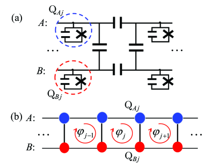
Figure 1: Schematic diagram of two-leg (labeled respectively by $A$ and $B$) superconducting circuits with the transmon qubits. All transmon qubits are coupled with their nearest-neighbor sites by capacitors. (a) Illustration of the detail circuit of a unit plaquette. Q_νj denotes the qubit at the $j$th site on the $\nu$th leg. (b) Schematic diagram of the two-leg lattice with an effective magnetic flux per plaquette which can be controlled independently. The blue and red solid spheres indicate respectively the transmon qubits at the $A$ and $B$ legs.

II Synthetic gauge field

As shown in Fig. 1(a), we consider the same experimental setup about two-leg superconducting circuits with the transmon qubits YY19 , whose dynamics is governed by a Bose-Hubbard ladder Hamiltonian

$$\hat{H}_{BH} = \sum_{\nu j}\omega_{\nu j}^{0}\hat{a}_{\nu j}^{{\dagger}}\hat{a}_{\nu j}+\sum_{\nu j}\frac{V_{\nu j}}{2}\hat{n}_{\nu j}\left(\hat{n}_{\nu j}-1\right)$$ (1)

$$+\sum_{\nu j}\left(g_{\nu j}\hat{a}_{\nu(j-1)}^{{\dagger}}\hat{a}_{\nu j}+\text{H.c.}\right)$$

$$+\sum_{j}\left(\tilde{g}_{j}\hat{a}_{Aj}^{{\dagger}}\hat{a}_{Bj}+\text{H.c.}\right),$$

where $j$ is the number of the rung, $\nu\in\{A,B\}$ labels the leg, the operator $\hat{a}_{\nu j}^{{\dagger}}$ ($\hat{a}_{\nu j}$) creates (annihilates) a photon at the $j$th site on the $\nu$th leg, $\hat{n}_{\nu j}=\hat{a}_{\nu j}^{{\dagger}}\hat{a}_{\nu j}$ is the number operator, $\omega_{\nu j}^{0}$ is the qubit frequency, $V_{\nu j}$ is the on-site attractive interaction at the $j$th site on the $\nu$th leg, $g_{\nu j}$ is the hopping strength between the nearest-neighbor sites along the leg $\nu$, $\tilde{g}_{j}$ is the interleg hopping strength at the rung $j$, and H.c. is the Hermitian conjugate. In experiment YY19 , the transmon qubit has a strong anharmonicity, $\left|V_{\nu j}\right|/g_{\nu j}\simeq 20$, which allows that only one photon can be excited at each site. In such case, the nonlinear term of the Hamiltonian (1) can be safely neglected.

To obtain the wanted synthetic gauge field, here we introduce an ac microwave driving in each transmon qubit, which is experimentally feasible through the flux-bias line TF . In this case, each qubit frequency is modulated independently as

$$\omega_{\nu j}(t)=\omega_{\nu j}^{0}+\varepsilon_{\nu j}\sin\left(u_{\nu j}t+\varphi_{\nu j}\right),$$ (2)

where $\varepsilon_{\nu j}$, $u_{\nu j}$ and $\varphi_{\nu j}$ are the driving amplitude, frequency and phase, respectively. By applying the rotation frame with an unitary operator $\hat{U}=\hat{U}_{1}\times\hat{U}_{2}$, where

$$\hat{U}_{1}=\exp\left[-i\sum_{\nu j}\omega_{\nu j}^{0}\hat{n}_{\nu j}t\right],$$ (3a)

$$\hat{U}_{2}=\exp\left[i\sum_{\nu j}\hat{n}_{\nu j}\alpha_{\nu j}\cos\left(u_{\nu j}t+\varphi_{\nu j}\right)\right],$$ (3b)

with $\alpha_{\nu j}=\varepsilon_{\nu j}/u_{\nu j}$, the transformed Hamiltonian

$$\hat{H}_{t}=\hat{U}^{{\dagger}}\hat{H}_{BH}\hat{U}+i\frac{d\hat{U}^{{\dagger}}}{dt}\hat{U}$$ (4)

can be divided into two parts as $\hat{H}_{t}=\hat{H}_{\text{E}}+\hat{H}_{\text{AB}}$, with

$$\hat{H}_{\text{E}} = \underset{\nu}{\sum}g_{\nu 1}\left\{\hat{a}_{\nu 1}^{{\dagger}}\hat{a}_{\nu 2}e^{-i\Delta_{\nu 2}t}\exp\left[-i\alpha_{\nu 1}\cos\left(u_{\nu 1}t+\varphi_{\nu 1}\right)\right]\exp\left[i\alpha_{\nu 2}\cos\left(u_{\nu 2}t+\varphi_{\nu 2}\right)\right]+\text{H.c.}\right\}$$ (5a)

$$+\underset{\nu}{\sum}g_{\nu 2}\left\{\hat{a}_{\nu 2}^{{\dagger}}\hat{a}_{\nu 3}e^{-i\Delta_{\nu 3}t}\exp\left[-i\alpha_{\nu 2}\cos\left(u_{\nu 2}t+\varphi_{\nu 2}\right)\right]\exp\left[i\alpha_{\nu 3}\cos\left(u_{\nu 3}t+\varphi_{\nu 3}\right)\right]+\text{H.c.}\right\}+...,$$

$$\hat{H}_{\text{AB}} = \tilde{g}_{1}\left\{\hat{a}_{A1}^{{\dagger}}\hat{a}_{B1}e^{-i\Delta_{AB1}t}\exp\left[-i\alpha_{A1}\cos\left(u_{A1}t+\varphi_{A1}\right)\right]\exp\left[i\alpha_{B1}\cos\left(u_{B1}t+\varphi_{B1}\right)\right]+\text{H.c.}\right\}$$ (5b)

$$+\tilde{g}_{2}\left\{\hat{a}_{A2}^{{\dagger}}\hat{a}_{B2}e^{-i\Delta_{AB2}t}\exp\left[-i\alpha_{A2}\cos\left(u_{A2}t+\varphi_{A2}\right)\right]\exp\left[i\alpha_{B2}\cos\left(u_{B2}t+\varphi_{B2}\right)\right]+\text{H.c.}\right\}+...,$$

with $\Delta_{\nu j}=\omega_{\nu j}^{0}-\omega_{\nu j-1}^{0}$ and $\Delta_{ABj}=\omega_{Bj}^{0}-\omega_{Aj}^{0}$. Using the Jacobi-Anger identity, $\exp\left[i\alpha\cos\left(ut+\varphi\right)\right]=\sum_{-\infty}^{\infty}i^{m}J_{m}(\alpha)\exp\left[im\left(ut+\varphi\right)\right]$, where $J_{m}(\alpha)$ is the Bessel function of the first kind, we have

$$\hat{H}_{\text{E}} = \underset{\nu j}{\sum}g_{\nu j}\hat{a}_{\nu\left(j-1\right)}^{{\dagger}}\hat{a}_{\nu j}\underset{m_{1}=-\infty}{\overset{\infty}{\sum}}(-i)^{m_{1}}J_{m_{1}}(\alpha_{\nu\left(j-1\right)})\exp\left[-im_{1}\left(u_{\nu\left(j-1\right)}t+\varphi_{\nu\left(j-1\right)}\right)\right]$$ (6a)

$$\times\underset{m_{2}=-\infty}{\overset{\infty}{\sum}}i^{m_{2}}J_{m_{2}}(\alpha_{\nu j})\exp\left[i\left(m_{2}u_{\nu j}-\Delta_{\nu j}\right)t+m_{2}\varphi_{\nu j}\right]+\text{H.c.},$$

$$\hat{H}_{\text{AB}} = \underset{j}{\sum}\tilde{g}_{j}\hat{a}_{Aj}^{{\dagger}}\hat{a}_{Bj}\underset{m_{1}=-\infty}{\overset{\infty}{\sum}}(-i)^{m_{1}}J_{m_{1}}(\alpha_{Aj})\exp\left[-im_{1}\left(u_{Aj}t+\varphi_{Aj}\right)\right]$$ (6b)

$$\times\underset{m_{2}=-\infty}{\overset{\infty}{\sum}}i^{m_{2}}J_{m_{2}}(\alpha_{Bj})\exp\left[i\left(m_{2}u_{Bj}-\Delta_{ABj}\right)t+m_{2}\varphi_{Bj}\right]+\text{H.c.}.$$

When choosing $\Delta_{\nu j}=u_{\nu j}$ ($-u_{\nu j}$) for odd (even) $j$ and $\Delta_{ABj}=u_{Bj}$, and considering the case that $u_{\nu j}\gg\left\{g_{\nu j},\tilde{g}_{j}\right\}$, the oscillating terms in Eqs. (6a) and (6b) are neglected by applying the rotating-wave approximation. Finally, the effective Hamiltonian is given by

$$\hat{H} = \underset{\nu j}{\sum}\left(t_{\nu j}e^{i\tilde{\varphi}_{\nu j}}\hat{a}_{\nu\left(j-1\right)}^{{\dagger}}\hat{a}_{\nu j}+\text{H.c.}\right)$$ (7)

$$+\underset{j}{\sum}\left(\tilde{t}_{j}e^{i\tilde{\varphi}_{Bj}}\hat{a}_{Aj}^{{\dagger}}\hat{a}_{Bj}+\text{H.c.}\right),$$

where $t_{\nu j}=g_{\nu j}J_{0}(\alpha_{\nu j-1})J_{1}(\alpha_{\nu j})$, $\tilde{t}_{j}=\tilde{g}_{j}J_{0}(\alpha_{Aj})J_{1}(\alpha_{Bj})$ with $J_{m}(\alpha)$ being the Bessel function of the first kind, and $\tilde{\varphi}_{\nu j}=\left(-1\right)^{j+1}\varphi_{\nu j}+\pi/2$.

The Hamiltonian in Eq. (7) shows clearly that the driving phase $\tilde{\varphi}_{\nu j}$ leads to complex hopping between any two nearest-neighbor sites, and thus make each plaquette accumulate a gauge-invariant magnetic flux $\varphi_{j}=\tilde{\varphi}_{Aj}-\tilde{\varphi}_{B\left(j-1\right)}\$, see Fig. 1(b). This synthetic magnetic flux per plaquette can be tuned independently by choosing the driving phases in the transmon qubits, which is better than the previous realizations in other systems. If choosing $\varphi_{j}=\varphi$, the uniform flux is formed DH14 ; MP15 ; ATOM-MA2 ; if $\varphi_{j}=(-1)^{j}\varphi$, the staggered flux is generated RS18 ; ATOM-MA ; LK10 ; GM10 ; MA13 ; if $\varphi_{j}=j\varphi$, the site-dependent flux is achieved ATOM-MA1 ; PC1 ; ATOM-BKS ; ATOM-HM .

III Ground-state chiral currents

The synthetic magnetic flux achieved can generate rich quantum phenomena. As an example, we investigate the experimentally-measurable ground-state chiral currents and chiral dynamics of the ladder system. For simplicity, we set $\alpha_{\nu j}=\alpha$ and $g_{\nu j}=\tilde{g}_{j}=g$, which mean that $t_{\nu j}=\tilde{t}_{j}=t_{0}=gJ_{0}(\alpha)J_{1}(\alpha)$. The driving phases are taken as $\tilde{\varphi}_{Aj}=-\tilde{\varphi}_{Bj}=\varphi/2$, and the synthetic magnetic flux thus becomes $\varphi_{j}=\varphi$. In this section, we mainly discuss the ground-state chiral currents. The case of single-qubit excitation is firstly considered and the case of two-qubit excitation is then addressed briefly.

By performing the Fourier transformation $\hat{a}_{\nu k}=\sum_{j}e^{ikj}\hat{a}_{\nu j}/\sqrt{N}$, where $N$ is the number of the ladder rungs, the Hamiltonian in Eq. (7) becomes $\hat{H}=\sum_{k}(\hat{a}_{Ak}^{{\dagger}},\hat{a}_{Bk}^{{\dagger}})\hat{h}(k)\left(\begin{array}[]{c}\hat{a}_{Ak}\\ \hat{a}_{Bk}\end{array}\right)$, where

$$\hat{h}(k)=\varepsilon_{0}(k)\mathit{\hat{I}}+t_{0}\hat{\sigma}_{x}+\varepsilon_{z}(k)\hat{\sigma}_{z}.$$ (8)

where $\mathit{\hat{I}}$ is the identity operator, $\hat{\sigma}_{x}$ and $\hat{\sigma}_{z}$ are the Pauli spin operators in the $x$ and $z$ directions, $\varepsilon_{0}(k)=2t_{0}\cos(\varphi/2)\cos k$, and $\ \varepsilon_{z}(k)=2t_{0}\sin(\varphi/2)\sin\left(k\right)$. Since the $A$ and $B$ legs act respectively as the spin-up and spin-down components, the $\hat{\sigma}_{x}$ term governs the tunneling between two legs. While the $\hat{\sigma}_{z}$ term, determined by the non-zero magnetic flux $\varphi$, generates spin-momentum locking that the spin-up and spin-down photons minimize their energies by having the positive and negative momenta, respectively. The Hamiltonian in Eq. (8) exhibits the time-reversal invariance DH14 , which leads to the Kramers degeneracy of the ground state, as will be shown below.

With the diagonalization of the momentum-space Hamiltonian in Eq. (8), we obtain two energy bands

$$E(k)=\varepsilon_{0}(k)\pm\sqrt{\varepsilon_{z}(k)^{2}+t_{0}^{2}},$$ (9)

which are plotted, in Fig. 2, as functions of the momentum $k$ for (a) $\varphi=0.1\pi$ and (b) $\varphi=0.9\pi$. For small $\varphi$, the lower energy band only has one minimum at $k=\pi$ or $k=-\pi$, as shown in Fig. 2(a). With increasing $\varphi$, two Kramers degeneracy points occur at $k=\pm q$, with

$$q=\frac{1}{2}\arccos\left\{\frac{1+\cos\left(\varphi\right)}{2\left[1-\cos\left(\varphi\right)\right]}+\cos\left(\varphi\right)\right\},$$ (10)

as shown in Fig. 2(b). The critical point that the lower energy band changes from one minimum to two minima is given by $\varphi_{c}=2\arccos(\sqrt{17}/4-1/4)$. For simplicity, here we choose $\varphi\in(0,\pi]$.

With single-qubit excitation, the eigenfunction of the lower energy band is obtained by

$$\left|\psi_{Lk}\right\rangle=\left(\alpha_{Lk}\hat{a}_{kA}^{{\dagger}}+\beta_{Lk}\hat{a}_{kB}^{{\dagger}}\right)\left|0\right\rangle,$$ (11)

where $\left|0\right\rangle$ is the vacuum state,

$$\alpha_{Lk} = \frac{(\bar{\varepsilon}_{z}-\sqrt{1+\bar{\varepsilon}_{z}^{2}})}{\sqrt{[(\bar{\varepsilon}_{z}-\sqrt{1+\bar{\varepsilon}_{z}^{2}})^{2}+1]}},$$ (12a)

$$\beta_{Lk} = \frac{1}{\sqrt{[(\bar{\varepsilon}_{z}-\sqrt{1+\bar{\varepsilon}_{z}^{2}})^{2}+1]}},$$ (12b)

with $\bar{\varepsilon}_{z}=2\sin(\varphi/2)\sin k$. In terms of Eq. (11), we have

$$\left\langle\hat{\sigma}_{z}\right\rangle_{Lk}=\frac{\left[\bar{\varepsilon}_{z}-\sqrt{1+\bar{\varepsilon}_{z}^{2}}\right]^{2}-1}{\left[\bar{\varepsilon}_{z}-\sqrt{1+\bar{\varepsilon}_{z}^{2}}\right]^{2}+1}.$$ (13)

Equation (13) shows clearly that when $k>0$ (i.e., $\bar{\varepsilon}_{z}>0$), $\left\langle\hat{\sigma}_{z}\right\rangle_{Lk}<0$, and vice versa, which indicates the spin-momentum locking effect induced by the non-zero magnetic flux. When $\varphi=0$, $\left\langle\hat{\sigma}_{z}\right\rangle_{Lk}\equiv 0$ for any $k$.

Figure 2: The energy bands as functions of the momentum $k$ for (a) $\varphi=0.1\pi$ and (b) $\varphi=0.9\pi$. The color indicates the value of $\left\langle\hat{\sigma}_{z}\right\rangle_{k}$.

Due to the spin-momentum locking, the photons in the $A$ leg move towards the left, whereas the photons in the $B$ leg move towards the right. As a result, the ladder system with non-zero magnetic flux exhibits a chiral current defined as

$$\hat{J}_{C}=\hat{J}_{A}-\hat{J}_{B},$$ (14)

with $\hat{J}_{A}=\sum_{j}\hat{J}_{Aj}$ and $\hat{J}_{B}=\sum_{j}\hat{J}_{Bj}$, where

$$\hat{J}_{Aj} = it_{0}e^{i\frac{\varphi}{2}}\hat{a}_{Aj}^{{\dagger}}\hat{a}_{A\left(j+1\right)}+\text{H.c.,}$$ (15a)

$$\hat{J}_{Bj} = it_{0}e^{-i\frac{\varphi}{2}}\hat{a}_{Bj}^{{\dagger}}\hat{a}_{B\left(j+1\right)}+\text{H.c..}$$ (15b)

On the other hand, since the $\hat{\sigma}_{x}$ term in the Hamiltonian in Eq. (8) governs the tunneling between two legs, it is necessary to define the current at the rung $j$ as

$$\hat{J}_{j}=it_{0}\hat{a}_{Aj}^{{\dagger}}\hat{a}_{Bj}+\text{H.c.}.$$ (16)

In terms of Eqs. (14)-(16), we can investigate the ground-state currents. For $\varphi<\varphi_{c}$, i.e., the lower energy band has one minimum, the ground-state wavefunction $\left|\psi_{\text{G}}\right\rangle=\left|\psi_{L\pi}\right\rangle$, whose corresponding currents are calculated as

$$\left\langle\hat{J}_{Aj}\right\rangle_{L\pi} = -\left\langle\hat{J}_{Bj}\right\rangle_{L\pi}=\frac{t_{0}}{N}\sin(\frac{\varphi}{2}),$$ (17a)

$$\left\langle\hat{J}_{C}\right\rangle_{L\pi} = 2t_{0}\sin(\frac{\varphi}{2}),$$ (17b)

$$\left\langle\hat{J}_{j}\right\rangle_{L\pi} = 0.$$ (17c)

These equations show that the currents along the $A$ and $B$ legs have opposite directions but with the same magnitudes, i.e., a non-zero chiral current is generated, while the current at the rung $j$ vanishes. This phenomenon clearly characterizes the Meissner effect EO01 .

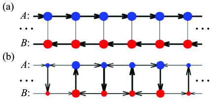
Figure 3: The currents between neighboring sites for (a) $\varphi=0.1\pi$ and (b) $\varphi=0.9\pi$ when $N=50$. The thicknesses of the arrows indicate their strengths. The sizes of the blue and red solid spheres denote the local densities at rungs on the $A$ and $B$ legs, respectively.

For $\varphi>\varphi_{c}$, i.e., the lower energy band has two minima, the ground-state wavefunction becomes $\left|\psi_{\text{G}}\right\rangle=\left(\left|\psi_{L\left(-q\right)}\right\rangle+\left|\psi_{Lq}\right\rangle\right)/\sqrt{2}$. In this case, the ground-state currents are given by

$$\left\langle\hat{J}_{Aj}\right\rangle_{Lq} = \frac{t_{0}}{N}\left[\alpha_{L(-q)}^{2}\sin\left(q-\frac{\varphi}{2}\right)-\alpha_{Lq}^{2}\sin\left(q+\frac{\varphi}{2}\right)\right.$$ (18a)

$$\left.-2\alpha_{L(-q)}\alpha_{Lq}\sin\left(\frac{\varphi}{2}\right)\cos\left(q+2qj\right)\right],$$

$$\left\langle\hat{J}_{Bj}\right\rangle_{Lq} = \frac{t_{0}}{N}\left[\beta_{L(-q)}^{2}\sin\left(q+\frac{\varphi}{2}\right)-\beta_{Lq}^{2}\sin\left(q-\frac{\varphi}{2}\right)\right.$$ (18b)

$$\left.+2\beta_{L(-q)}\beta_{Lq}\sin\left(\frac{\varphi}{2}\right)\cos\left(q+2qj\right)\right],$$

$$\left\langle\hat{J}_{C}\right\rangle_{Lq} = t_{0}\left[\alpha_{Lq}^{2}\sin\left(\frac{\varphi}{2}+q\right)-\alpha_{L(-q)}^{2}\sin\left(q-\frac{\varphi}{2}\right)\right.$$

$$\left.-\beta_{Lq}^{2}\sin\left(q-\frac{\varphi}{2}\right)+\beta_{L(-q)}^{2}\sin\left(\frac{\varphi}{2}+q\right)\right],$$

$$\left\langle\hat{J}_{j}\right\rangle_{Lq} = \frac{t_{0}}{N}\sin\left(2qj\right)\left[\alpha_{Lq}\beta_{L(-q)}-\alpha_{L(-q)}\beta_{Lq}\right].$$

Since $\alpha_{L(-q)}=-\beta_{Lq}$ and $\alpha_{Lq}=-\beta_{L(-q)}$, it is easy to verify that $\left\langle\hat{J}_{Aj}\right\rangle_{Lq}=$ $-\left\langle\hat{J}_{Bj}\right\rangle_{Lq}$. Equations (18a), (18b) and (LABEL:JJQ) show that the currents between any two nearest-neighbor sites vary periodically when increasing $j$, characterizing the vortex current EO17 .

In Fig. 3, we plot the currents between any two nearest-neighbor sites for (a) $\varphi=0.1\pi$ and (b) $\varphi=0.9\pi$, which support the above analytical results. While in Fig. 4(a), we plot the ground-state chiral current as a function of $\varphi$. With increasing $\varphi$, this chiral current firstly increases to a maximal value at the critical point $\varphi_{c}$ and then decreases, which characterizes a transition from the Meissner phase to the vortex phase MP15 ; RS18 . For a finite size, this transition feature still remains but the critical point changes slightly, which means that the Meissner and vortex phases as well as their transition can be observed in current experimental setup. In Fig. 4(b), we plot the ground-state chiral current for two-qubit excitations, which has similar properties as those with single-qubit excitation.

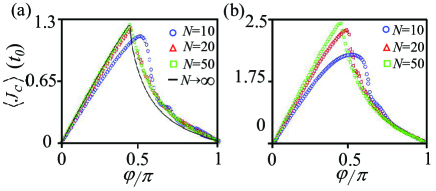
Figure 4: The ground-state chiral currents as functions of $\varphi$ for (a) single-qubit and (b) two-qubit excitations. The solid line in (a) is the analytical result from Eq. (LABEL:JC2). The hollow blue circles, red triangles and green squares are the results of $N=10$, 20 and 50, respectively.

IV Chiral dynamics

We now investigate the chiral dynamics of the Hamiltonian in Eq. (7) with $N=10$ and $\varphi=0.5\pi$. For simplify, we set $t_{0}=1$ in the following discussion. We first consider the case of single-qubit excitation denoted by $\hat{a}_{\nu j}^{{\dagger}}\left|0\right\rangle$, which describes that the qubit at the $j$th site on the$\ \nu$th leg is excited. In Fig. 5, we plot the density distributions of photons at each site of the ladder for $t=0$ and $t=1$, when the initial states are prepared respectively as $\left|\psi(0)\right\rangle_{1\text{S}}=(\hat{a}_{A5}^{{\dagger}}+\hat{a}_{B5}^{{\dagger}})$ $\left|0\right\rangle/\sqrt{2}$ (a₁,a₂) , $\left|\psi(0)\right\rangle_{1\text{AS}}=(\hat{a}_{A5}^{{\dagger}}-\hat{a}_{B5}^{{\dagger}})\left|0\right\rangle/\sqrt{2}$ (b₁,b₂), and $\left|\psi(0)\right\rangle_{1\text{E}}=\hat{a}_{B5}^{{\dagger}}\left|0\right\rangle$ (c₁,c₂). This figure shows that for the initial state $\left|\psi(0)\right\rangle_{1\text{S}}$, the most photons move to the left (right) of the central rung on the $A$ $(B)$ leg [see Fig. 5(a₂)], which characterizes chiral dynamics. The converse occurs for the initial state $\left|\psi(0)\right\rangle_{1\text{AS}}$ [see Fig. 5(b₂)]. While for the initial state $\left|\psi(0)\right\rangle_{1\text{E}}$, the photons simultaneously move to the both sides of the central rung [see Fig. 5(c₂)], i.e., the chiral dynamics disappears. In order to see these results clearly, we consider a short-time ($\delta t$) dynamics, in which the time-dependent wavefunction is obtained, up to second order, as $\left|\psi(\delta t)\right\rangle\simeq[1-i\hat{H}\delta t-(\hat{H}\delta t)^{2}/2]\left|\psi(0)\right\rangle$. As a result, the differences between the photons moving to the right and left of the center rung on the $A$ and $B$ legs under these three initial states are given respectively by

$$\left\langle\Delta\hat{n}_{A}\right\rangle_{1\text{S}}=-\left\langle\Delta\hat{n}_{B}\right\rangle_{1\text{S}}=\delta t^{3}\sin(\varphi),$$ (19a)

$$\left\langle\Delta\hat{n}_{A}\right\rangle_{1\text{AS}}=-\left\langle\Delta\hat{n}_{B}\right\rangle_{1\text{AS}}=-\delta t^{3}\sin(\varphi),$$ (19b)

$$\left\langle\Delta\hat{n}_{A}\right\rangle_{1\text{E}}=\left\langle\Delta\hat{n}_{B}\right\rangle_{1\text{E}}\text{ }=0,$$ (19c)

where $\Delta\hat{n}_{A}=\overset{4}{\sum_{j=1}}\hat{n}_{Aj}-\overset{10}{\sum_{j=6}}\hat{n}_{Aj}$ and $\Delta\hat{n}_{B}=\overset{4}{\sum_{j=1}}\hat{n}_{Bj}-\overset{10}{\sum_{j=6}}\hat{n}_{Bj}$. Equations (19a) and (19b) show clearly that for the initial states $\left|\psi(0)\right\rangle_{1\text{S}}$ and $\left|\psi(0)\right\rangle_{1\text{AS}}$, the opposite differences are raised by non-zero $\varphi$, and the chiral dynamics can thus be formed. While for the initial state $\left|\psi(0)\right\rangle_{1\text{E}}$, both differences disappears [see Eq. (19c)], i.e., no chiral dynamics occurs.

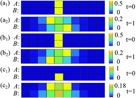
Figure 5: The density distributions of photons at each site with single-qubit excitation for the different initial states $\left|\psi(0)\right\rangle_{1\text{S}}$ $=(\hat{a}_{A5}^{{\dagger}}+\hat{a}_{B5}^{{\dagger}})$ $\left|0\right\rangle/\sqrt{2}$ with (a₁) $t=0$ and (a₂) $t=1$, $\left|\psi(0)\right\rangle_{1\text{AS}}=(\hat{a}_{A5}^{{\dagger}}-\hat{a}_{B5}^{{\dagger}})\left|0\right\rangle/\sqrt{2}$ with (b₁) $t=0$ and (b₂) $t=1$, and $\left|\psi(0)\right\rangle_{1\text{E}}=\hat{a}_{B5}^{{\dagger}}\left|0\right\rangle$ with (c₁) $t=0$ and (c₂) $t=1$. In all subfigures, the synthetic magnetic flux $\varphi=0.5\pi$.

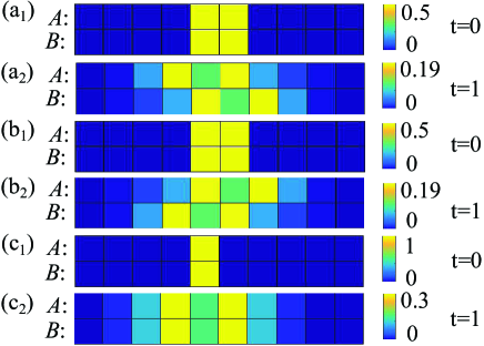
Figure 6: The density distributions of photons at each site with two-qubit excitations for the different initial states $\left|\psi(0)\right\rangle_{2\text{S}}=(\hat{a}_{A5}^{{\dagger}}+\hat{a}_{B5}^{{\dagger}})(\hat{a}_{A6}^{{\dagger}}+\hat{a}_{B6}^{{\dagger}})\left|0\right\rangle/2$ with (a₁) $t=0$ and (a₂) $t=1$, $\left|\psi(0)\right\rangle_{2\text{AS}}=(\hat{a}_{A5}^{{\dagger}}-\hat{a}_{B5}^{{\dagger}})(\hat{a}_{A6}^{{\dagger}}-\hat{a}_{B6}^{{\dagger}})\left|0\right\rangle/2$ with (b₁) $t=0$ and (b₂) $t=1$, and $\left|\psi(0)\right\rangle_{2\text{E}}=\hat{a}_{A5}^{{\dagger}}\hat{a}_{B5}^{{\dagger}}\left|0\right\rangle$ with (c₁) $t=0$ and (c₂) $t=1$. In all subfigures, the synthetic magnetic flux $\varphi=0.5\pi$.

These results can be understood by considering the properties of both two energy bands shown in Fig. 2. The fundamental information of the lower band has been given in the previous section. While for the upper energy band, its eigenfunction is given by

$$\left|\psi_{Uk}\right\rangle=\left(\alpha_{Uk}\hat{a}_{kA}^{{\dagger}}+\beta_{Uk}\hat{a}_{kB}^{{\dagger}}\right)\left|0\right\rangle,$$ (20)

where

$$\alpha_{Uk} = \frac{(\bar{\varepsilon}_{z}+\sqrt{1+\bar{\varepsilon}_{z}^{2}})}{\sqrt{[(\bar{\varepsilon}_{z}+\sqrt{1+\bar{\varepsilon}_{z}^{2}})^{2}+1]}},$$ (21a)

$$\beta_{Uk} = \frac{1}{\sqrt{[(\bar{\varepsilon}_{z}+\sqrt{1+\bar{\varepsilon}_{z}^{2}})^{2}+1]}}.$$ (21b)

From Eqs. (11) and (20), we obtain

$$\hat{a}_{Ak}^{{\dagger}}\left|0\right\rangle = -\alpha_{L\left(-k\right)}\left|\psi_{Uk}\right\rangle+\alpha_{Lk}\left|\psi_{Lk}\right\rangle,$$ (22a)

$$\hat{a}_{Bk}^{{\dagger}}\left|0\right\rangle = -\alpha_{L(-k)}\left|\psi_{Uk}\right\rangle-\alpha_{Lk}\left|\psi_{Lk}\right\rangle,$$ (22b)

where the relations $\alpha_{Uk}=\beta_{Lk}$, $\beta_{Uk}=-\alpha_{Lk}$ and $\alpha_{L\left(-k\right)}=-\beta_{Lk}$ have been used. In terms of Eqs. (22a) and (22b), the three initial states we have chosen are rewritten as

$$\left|\psi(0)\right\rangle_{1\text{S}} = -\sum_{k}\sqrt{2}e^{i5k}\alpha_{L\left(-k\right)}\left|\psi_{Uk}\right\rangle,$$ (23a)

$$\left|\psi(0)\right\rangle_{1\text{AS}} = -\sum_{k}\sqrt{2}e^{i5k}\alpha_{Lk}\left|\psi_{Lk}\right\rangle,$$ (23b)

$$\left|\psi(0)\right\rangle_{1\text{E}}\! = \!-\sum_{k}\!e^{i5k}\!\left(\!\alpha_{L(-k)}\!\left|\psi_{Uk}\right\rangle\!+\!\alpha_{Lk}\!\left|\psi_{Lk}\right\rangle\!\right)\!.$$ (23c)

Equations (23a) and (23b) show clearly that for the symmetric (antisymmetric) initial state $\left|\psi(0)\right\rangle_{1\text{S}}$ ($\left|\psi(0)\right\rangle_{1A\text{S}}$), the photons only populate the upper (lower) band. Due to the spin-momentum locking effect in the two bands, the chiral dynamics occurs. Equation (23c) shows that when the initial state is chosen as $\left|\psi(0)\right\rangle_{1\text{E}}$, the photons populate equally the upper and lower bands with opposite $k$. Since the two energy bands have opposite chirality (see Fig. 2), the photons move to the both sides of their initial positions simultaneously and the chiral dynamics thus disappears.

In Fig 6, we plot the density distributions of photons at $t=0$ and $t=1$ for two-qubit excitations of $\hat{a}_{\nu j}^{{\dagger}}\hat{a}_{\nu^{\prime}j^{\prime}}^{{\dagger}}\left|0\right\rangle$, which describes that the qubits at the $j$th site on the $\nu$th leg and at the $j^{\prime}$th site on the $\nu^{\prime}$th leg are excited. We emphasize that $\nu$ and $\nu^{\prime}$, $j$ and $j^{\prime}$ are not equal simultaneously. The initial states are chosen respectively as $\left|\psi(0)\right\rangle_{2\text{S}}=(\hat{a}_{A5}^{{\dagger}}+\hat{a}_{B5}^{{\dagger}})(\hat{a}_{A6}^{{\dagger}}+\hat{a}_{B6}^{{\dagger}})\left|0\right\rangle/2$ (a₁,a₂), $\left|\psi(0)\right\rangle_{2\text{AS}}=(\hat{a}_{A5}^{{\dagger}}-\hat{a}_{B5}^{{\dagger}})(\hat{a}_{A6}^{{\dagger}}-\hat{a}_{B6}^{{\dagger}})\left|0\right\rangle/2$ (b₁,b₂), and $\left|\psi(0)\right\rangle_{2\text{E}}=\hat{a}_{A5}^{{\dagger}}\hat{a}_{B5}^{{\dagger}}\left|0\right\rangle$ (c₁,c₂). This figure shows the similar conclusions as those with single-qubit excitation, i.e., for the initial states $\left|\psi(0)\right\rangle_{2\text{S}}$ and $\left|\psi(0)\right\rangle_{2\text{AS}}$, the system has opposite chiral dynamics, which disappears for the initial state $\left|\psi(0)\right\rangle_{2\text{E}}$.

Figure 7: The interleg hopping strength as a function of the parameters $\alpha_{Aj}$ and $\alpha_{Bj}$.

V Possible experimental observation

In this section, we briefly discuss how to detect the ground-state chiral current and the chiral dynamics in experiments. To observe the ground-state chiral current, we firstly turn off the parameters $t_{0}$ and $\varphi$ and prepare the corresponding system in its single-qubit (two-qubit) excitation state $\hat{a}_{\nu j}^{{\dagger}}\left|0\right\rangle$ ($\hat{a}_{\nu j}^{{\dagger}}\hat{a}_{\nu^{\prime}j^{\prime}}^{{\dagger}}\left|0\right\rangle$) by the microwave driving. Then, we adiabatically turn on these parameters to achieve the ground state of the system by the Landau-Zener theorem LZ . Based on the state tomography that has been developed successfully ST , the density of the states at each site can be measured and the matrix density $\hat{\rho}$ is thus constructed. This indicates that the ground-state chiral current can be obtained by $\left\langle\hat{J}_{C}\right\rangle=tr(\hat{\rho}\hat{J}_{C})$ PR17 , where $tr$ is the trace operator. If the ground-state chiral current increases (decreases) as the magnetic flux increases, the Meissner (vortex) phase is found.

To observe the chiral dynamics, preparing the corresponding initial states plays a crucial role. The initial state $\hat{a}_{B5}^{{\dagger}}\left|0\right\rangle$ ($\hat{a}_{A5}^{{\dagger}}\hat{a}_{B5}^{{\dagger}}\left|0\right\rangle$) can be prepared directly by the microwave driving. For the superposition state $(\hat{a}_{A5}^{{\dagger}}+\hat{a}_{B5}^{{\dagger}})$ $\left|0\right\rangle/\sqrt{2}$ [$(\hat{a}_{A5}^{{\dagger}}-\hat{a}_{B5}^{{\dagger}})\left|0\right\rangle/\sqrt{2}$], we firstly turn off all the phases and the hopping strengths between the $\nu 5$ site and its nearest neighbor sites, and prepare the system in the state $\hat{a}_{\nu 5}^{{\dagger}}\left|0\right\rangle$. Since the superposition state $(\hat{a}_{A5}^{{\dagger}}+\hat{a}_{B5}^{{\dagger}})$ $\left|0\right\rangle/\sqrt{2}$ [$(\hat{a}_{A5}^{{\dagger}}-\hat{a}_{B5}^{{\dagger}})\left|0\right\rangle/\sqrt{2}$] is the ground state of the isolate rung subsystem at $j=5$ with the negative (positive) interleg hopping strength, we adiabatically turn on the interleg hopping strength towards the negative (positive) by tuning the parameters $\alpha_{A5}$ and $\alpha_{B5}$ (see Fig. 7). As a result, the required superposition states are prepared. Similarly, in the case of two-qubit excitations, the initial superposition state $(\hat{a}_{A5}^{{\dagger}}+\hat{a}_{B5}^{{\dagger}})(\hat{a}_{A6}^{{\dagger}}+\hat{a}_{B6}^{{\dagger}})\left|0\right\rangle/2$ [$(\hat{a}_{A5}^{{\dagger}}-\hat{a}_{B5}^{{\dagger}})(\hat{a}_{A6}^{{\dagger}}-\hat{a}_{B6}^{{\dagger}})\left|0\right\rangle/2$] is the ground state of the subsystem with two isolate rungs at $j=5$ and $j=6$ with the negative (positive) interleg hopping strengths. We firstly turn off all the phases and hopping strengths between the $\nu j$ ($j=5$ and $j=6$) site and its nearest neighbor sites, and drive the system in the state $\hat{a}_{A5}^{{\dagger}}\hat{a}_{A6}^{{\dagger}}\left|0\right\rangle$. The required superposition states can be prepared by adiabatically turning on the interleg hopping strengths both at the $5$th and $6$th rungs via the parameters $\alpha_{A5}$, $\alpha_{B5}$, $\alpha_{A6}$ and $\alpha_{B6}$ (see Fig. 7). Then, the chiral dynamics of the system can be observed by performing quantum state tomography ST .

VI Conclusions

In summary, we have proposed an experimentally-feasible method to prepare the synthetic gauge field in the two-leg superconducting circuits with transmon qubits. In particular, the realized magnetic flux per plaquette is controlled independently by properly choosing the phases of the alternating-current microwave driving in each qubit, which is better than the previous realizations in the other quantum simulation systems. Moreover, we have obtained the ground-state chiral currents for the single- and two-qubit excitations and found the Meissner-vortex phase transition. In the Meissner (vortex) phase, the ground-state chiral current increases (decreases) as the magnetic flux increases. We have also explored the chiral dynamics, which depends crucially on the initial state of the system. Finally, the possible experimental observations of the chiral current and dynamics are addressed. Our results pave a new route to explore novel many-body properties SSN15 ; AK15 ; SG16 ; SG17 ; RS17 ; YZ17 ; RC18 ; MSC19 , which can be induced by the interplay of gauge field, two-leg hoppings and interaction of photons in superconducting circuits.

References

• (1) Z. L. Xiang, S. Ashhab, J. Q. You, and F. Nori, Rev. Mod. Phys. 85, 623 (2013).
• (2) X. Gu, A. F. Kockum, A. Miranowicz, Y. Liu, and F. Nori, Phys. Rep. 718, 1 (2017).
• (3) G. Wendin, Rep. Phys. 80, 106001 (2017).
• (4) A. Blais, S. M. Girvin, and W. D. Oliver, Nat. Phys. 16, 247 (2020).
• (5) I. Buluta, S. Ashhab, and F. Nori, Rep. Prog. Phys. 74, 104401 (2011).
• (6) F. Arute, K. Arya, R. Babbush, D. Bacon, J. C. Bardin, R. Barends, R. Biswas, S. Boixo, F. G. S. L. Brandao, D. A. Buell, et. al., Nature (London) 574, 505 (2019).
• (7) S. Schmidt and J. Koch, Ann. Phys. (Berlin) 525, 395 (2013).
• (8) I. M. Georgescu, S. Ashhab, and F. Nori, Rev. Mod. Phys. 86, 153 (2014).
• (9) I. Carusotto, A. A. Houck, A. J. Kollár, P. Roushan, D. I. Schuster, and J. Simon, Nat. Phys. 16, 268 (2020).
• (10) Y. Salathé, M. Mondal, M. Oppliger, J. Heinsoo, P. Kurpiers, A. Potočnik, A. Mezzacapo, U. Las Heras, L. Lamata, E. Solano, S. Filipp, and A. Wallraff, Phys. Rev. X 5, 021027 (2015).
• (11) A. Kandala, A. Mezzacapo, K. Temme, M. Takita, M. Brink, J. M. Chow, and J. M. Gambetta, Nature (London) 549, 242 (2017).
• (12) P. Roushan, C. Neill, J. Tangpanitanon, V. M. Bastidas, A. Megrant, R. Barends, Y. Chen, Z. Chen, B. Chiaro, A. Dunsworth, et. al., Science 358, 1175 (2017).
• (13) K. Xu, J. J. Chen, Y. Zeng, Y. R. Zhang, C. Song,W. X. Liu, Q. J. Guo, P. F. Zhang, D. Xu, H. Deng, et. al., Phys. Rev. Lett. 120, 050507 (2018).
• (14) P. J. J. O’Malley, R. Babbush, I. D. Kivlichan, J. Romero, J. R. McClean, R. Barends, J. Kelly, P. Roushan, A. Tranter, N. Ding, et. al., Phys. Rev. X 6, 031007 (2016).
• (15) Y. P. Zhong, D. Xu, P. Wang, C. Song, Q. J. Guo, W. X. Liu, K. Xu, B. X. Xia, C.-Y. Lu, S. Han, et. al., Phys. Rev. Lett. 117, 110501 (2016).
• (16) C. Song, D. Xu, P. Zhang, J. Wang, Q. Guo, W. Liu, K. Xu, H. Deng, K. Huang, D. Zheng, et. al., Phys. Rev. Lett. 121, 030502 (2018).
• (17) W. Cai, J. Han, F. Mei, Y. Xu, Y. Ma, X. Li, H. Wang, Y. P. Song, Z. Y. Xue, Z. Q. Yin, et. al., Phys. Rev. Lett. 123, 080501 (2019).
• (18) Z. Yan, Y. R. Zhang, M. Gong, Y. Wu, Y. Zheng, S. Li, C. Wang, F. Liang, J. Lin, Y. Xu, et. al., Science 364, 753 (2019).
• (19) R. Ma, B. Saxberg, C. Owens, N. Leung, Y. Lu, and J. Simon, Nature (London) 566, 51 (2019).
• (20) M. Fitzpatrick, N. M. Sundaresan, A. C. Y. Li, J. Koch, and A. A. Houck, Phys. Rev. X 7, 011016 (2017).
• (21) Y. Ye, Z. Y. Ge, Y. Wu, S. Wang, M. Gong, Y. R. Zhang, Q. Zhu, R. Yang, S. Li, F. Liang, et. al., Phys. Rev. Lett. 123, 050502 (2019).
• (22) D. N. Sheng, O. I. Motrunich, and M. P. A. Fisher, Phys. Rev. B 79, 205112 (2009).
• (23) H. H. Lai and O. I. Motrunich, Phys. Rev. B 81, 045105 (2010).
• (24) X. Li, E. Zhao, and W. V. Liu, Nat. Commun. 4, 1523 (2013).
• (25) W. M. Huang, K. Irwin, and S. W. Tsai, Phys. Rev. A 87, 031603(R)(2013).
• (26) S. Uchino and T. Giamarchi, Phys. Rev. A 91, 013604 (2015).
• (27) J. P. Lv and Z. D. Wang, Phys. Rev. B 93, 174507 (2016).
• (28) S. Greschner and F. H. Meisner, Phys. Rev. A 97, 033619 (2018).
• (29) R. Nehra, D. S. Bhakuni, S. Gangadharaiah, and A. Sharma, Phys. Rev. B 98, 045120 (2018).
• (30) Z. Zhou, F. Chen, Y. Zhong, H. G. Luo, and J. Zhao, Phys. Rev. B 99, 205143 (2019).
• (31) R. A. Santos and B. Béri, Phys. Rev. B 100, 235122 (2019).
• (32) G. L. Nave, K. Limtragool, and P. W. Phillips, Rev. Mod. Phys. 91, 021003 (2019).
• (33) D. Bailin and A. Love, Cosmology in gauge field theory and string theory (CRC Press, 2004).
• (34) J. Dalibard, F. Gerbier, G. Juzeliūnas, and P. Öhberg, Rev. Mod. Phys. 83, 1523 (2011).
• (35) N. Goldman, G. Juzeliūnas, Pohberg, and I. B. Spielman, Rep. Prog. Phys. 77, 126401 (2014).
• (36) D.-W. Zhang, Y.-Q. Zhu, Y. X. Zhao, H. Yan, and S.-L. Zhu, Adv. Phys. 67, 253 (2018).
• (37) E. Witten, Rev. Mod. Phys. 88, 035001 (2016).
• (38) Y.-P. Wang, W. Wang, Z.-Y. Xue, W.-L. Yang, Y. Hu, and Y. Wu, Sci. Rep. 5, 8352 (2015).
• (39) Y.-P. Wang, W.-L. Yang, Y. Hu, Z.-Y. Xue, and Y. Wu, npj Quantum Inf. 2, 16015 (2016).
• (40) P. Roushan, C. Neill, A. Megrant, Y. Chen, R. Babbush, R. Barends, B. Campbell, Z. Chen, B. Chiaro, A. Dunsworth, et. al., Nat. Phys. 13, 146 (2017).
• (41) D. W. Wang, C. Song, W. Feng, H. Cai, D. Xu, H. Deng, H. Li, D. Zheng, X. Zhu, H. Wang, et. al., Nat. Phys. 15, 382 (2019).
• (42) M. Aidelsburger, M. Atala, S. Nascimbène, S. Trotzky, Y. A. Chen and I. Bloch, Phys. Rev. Lett. 107, 255301 (2011).
• (43) M. Aidelsburger, M. Atala, M. Lohse, J. T. Barreiro, B. Paredes, and I. Bloch, Phys. Rev. Lett. 111, 185301 (2013).
• (44) H. Miyake, G. A. Siviloglou, C. J. Kennedy, W. C. Burton and W. Ketterle, Phys. Rev. Lett. 111, 185302 (2013).
• (45) M. Atala, M. Aidelsburger, M. Lohse, J. T. Barreiro, B. Paredes, and I. Bloch, Nat. Phys. 10, 588 (2014).
• (46) B. K. Stuhl, H. I. Lu, L. M. Aycock, D. Genkina, and I. B. Spielman, Science 349, 1514 (2015).
• (47) M. Mancini, G. Pagano, G. Cappellini, L. Livi, M. Rider, J. Catani, C. Sias, P. Zoller, M. Inguscio, M. Dalmonte, and L. Fallan, Science 349, 1510 (2015).
• (48) M. Hafezi, S. Mittal, J. Fan, A. Migdall, and J. M. Taylor, Nat. Photon. 7, 1001 (2013).
• (49) K. Fang, J. Luo, A. Metelmann, M. H. Matheny, F. Marquardt, A. A. Clerk, and O. Painter, Nat. Phys. 13, 465 (2017).
• (50) L. Yuan, Q. Lin, A. Zhang, M. Xiao, X. Chen, and S. Fan, Phys. Rev. Lett. 122, 083903 (2019).
• (51) Y. Chen, Y. L. Zhang, Z. Shen, C. L. Zou, G. C. Guo, and C. H. Dong, arXiv: 1908.04456 (2019).
• (52) X. Wen, C. Qiu, Y. Qi, L. Ye, M. Ke, F. Zhang, and Z. Liu, Nat. Phys. 15, 352 (2019).
• (53) A. Bermudez, T. Schaetz, and D. Porras, Phys. Rev. Lett. 107, 150501 (2011).
• (54) X. Li, Y. Ma, J. Han, T. Chen, Y. Xu, W. Cai, H. Wang, Y. P. Song, Z. Y. Xue, Z. Yin, and L. Sun, Phys. Rev. Appl. 10, 054009 (2018).
• (55) D. Hügel and B. Paredes, Phys. Rev. A 89, 023619 (2014).
• (56) M. Piraud, F. H. Meisner, I. P. McCulloch, S. Greschner, T. Vekua, and U. Schollwöck, Phys. Rev. B 91, 140406 (2015).
• (57) L. K. Lim, A. Hemmerich, and C. M. Smith, Phys. Rev. A 81, 023404 (2010).
• (58) G. Möller and N. R. Cooper, Phys. Rev. A 82, 063625 (2010).
• (59) M. Aidelsburger, M. Atala, S. Nascimb‘ene, S. Trotzky, Y. A. Chen, and I. Bloch, Appl. Phys. B 113, 1 (2013).
• (60) R. Sachdeva, F. Metz, M. Singh, T. Mishra, and T. Busch, Phys. Rev. A 98, 063612 (2018).
• (61) E. Orignac and T. Giamarchi, Phys. Rev. B 64, 144515 (2001).
• (62) E. Orignac, R. Citro, M. D. Dio, and S. D. Palo, Phys. Rev. B 96, 014518 (2017).
• (63) G. Zener, Proc. R. Soc. London, Ser. A 137, 696 (1932).
• (64) M. Steffen, M. Ansmann, R. McDermott, N. Katz, R. C. Bialczak, E. Lucero, M. Neeley, E. M. Weig, A. N. Cleland, and J. M. Martinis, Phys. Rev. Lett. 97, 050502 (2006).
• (65) S. S. Natu, Phys. Rev. A 92, 053623 (2015).
• (66) A. Keles and M. Ö. Oktel, Phys. Rev. A 91, 013629 (2015).
• (67) S. Greschner, M. Piraud, F. H. Meisner, I. P. McCulloch, U. Schollwöck, and T. Vekua1, Phys. Rev. A 94, 063628 (2016).
• (68) S. Greschner and T. Vekua, Phys. Rev. Lett. 119, 073401 (2017).
• (69) R. Sachdeva, M. Singh, and T. Busch, Phys. Rev. A 95, 063601 (2017).
• (70) Y. Zheng, S. Feng, and S. J. Yang, Phys. Rev. A 96, 063613 (2017).
• (71) R. Citro, S. D. Palo, M. D. Dio, and E. Orignac, Phys. Rev. B 97, 174523 (2018).
• (72) M. C. Strinati, S. Sahoo, K. Shtengel, and E. Sela, Phys. Rev. B 99, 245101 (2019).