Abstract

Tagging jets of strongly interacting particles initiated by energetic strange quarks is one of the few largely unexplored Standard Model object classification problems remaining in high energy collider physics. In this paper we investigate the purest version of this classification problem in the form of distinguishing strange-quark jets from down-quark jets. Our strategy relies on the fact that a strange-quark jet contains on average a higher ratio of neutral kaon energy to neutral pion energy than does a down-quark jet. Long-lived neutral kaons deposit energy mainly in the hadronic calorimeter of a high energy detector, while neutral pions decay promptly to photons that deposit energy mainly in the electromagnetic calorimeter. In addition, short-lived neutral kaons that decay in flight to charged pion pairs can be identified as a secondary vertex in the inner tracking system. Using these handles we study different approaches to distinguishing strange-quark from down-quark jets, including single variable cut-based methods, a boosted decision tree (BDT) with a small number of simple variables, and a deep learning convolutional neural network (CNN) architecture with jet images. We show that modest gains are possible from the CNN compared with the BDT or a single variable. Starting from jet samples with only strange-quark and down-quark jets, the CNN algorithm can improve the strange to down ratio by a factor of roughly 2 for strange tagging efficiencies below 0.2, and by a factor of 2.5 for strange tagging efficiencies near 0.02.

1 Introduction

Understanding jets, collimated collections of hadrons arising from strongly interacting particles produced in high-energy collisions, is a key ingredient of physics measurements and new physics searches at a high energy collider such as the Large Hadron Collider (LHC). One of the goals of jet reconstruction in a modern high energy collider detector is to use the observable properties of the jet to determine on average the identity of the strongly interacting particle that initiated the jet before QCD showering and hadronization.

Various methods for jet tagging have been developed over the years. Gluon jets tend to have more constituents with more uniform energy fragmentation and wider spread, as compared to light-quark jets, owing to their larger color factor (see e.g. Ref. [1] and references therein). For recent papers that apply machine learning to the problem of quark/gluon tagging, see Refs. [2, 3, 4, 5, 6, 7, 8]. Bottom- and charm-quark tagging can be achieved by looking for displaced charged track vertices [9, 10]. For up- versus down-quark tagging, the $p_{T}$-weighted track charge can offer some level of discrimination [11, 12, 13, 6]. Finally, if a top-quark is boosted, its decay products tend to be collimated into a large-radius jet that can be distinguished from quark/gluon jets by using jet mass or jet substructure variables such as N-subjettiness [14] (for a review of boosted top tagging and original references, see Ref. [15]). Recently, deep learning has been applied to the problem of boosted top-quark tagging with great success [16, 17, 18, 19, 20, 21, 22, 23, 24, 25, 26, 27, 28, 29, 30, 31].

The last largely unexplored type of jet tagging is for strange-quark jets. In this work, we investigate the possibilities for strange-quark jet tagging using observables that are available in the current generation of general purpose high energy collider detectors, such as the CMS and ATLAS detectors at the LHC. Strange-quark jet tagging at future $e^{+}e^{-}$ colliders has also recently been studied using Monte Carlo truth-level information [32]. Deployment of strange-quark jet tagging in the analysis of actual data from a high energy collider would of necessity be within the context of distinguishing among all types of prompt jets. In this demonstration-level work we restrict attention to the more restrictive problem of distinguishing strange- and down-quark jets. Jets initiated by these two types of quarks are most alike, and so the discrimination problem is most challenging.

Strange- and down-quarks have identical QCD and electromagnetic interactions, and so effectively only differ in hadronization and subsequent decay processes. As detailed below, the key difference at the hadronization level is that strange-quark jets have a larger momentum weighted fraction of kaon mesons than do down-quark jets. Long-lived neutral kaons deposit energy primarily in the hadronic calorimeter (HCAL) of a general purpose collider detector. In contrast, neutral pions, that are more common in down-quark jets, decay promptly to pairs of photons that deposit energy in the electromagnetic calorimeter (ECAL). So on average, a strange-quark jet has a somewhat larger neutral hadronic energy fraction, while a down-quark jet has a larger neutral electromagnetic energy fraction. This difference can provide a handle to on average distinguish strange- and down-quark jets. In addition, the momentum of short-lived neutral kaons that decay-in-flight to charged pion pairs within the inner tracking region can be reconstructed [33, 34] and this provides another handle to distinguish these types of jets.

We explore a number of strange- versus down-quark jet tagging algorithms based on observables available in the current generation of general purpose high energy collider detectors. These range from single whole-jet variables, to Boosted Decision Trees (BDTs) with a few whole-jet variables, to Convolutional Neutral Networks (CNNs) with jet images based on inputs from detector sub-systems. The CNNs provide modest gains in discrimination, with the best one making use of all of the available handles mentioned above.

Jet tagging algorithms have many applications in high energy collider physics. Sub-dividing events into categories based on tagging algorithm outputs can be used to isolate sought out signals from backgrounds, thereby increasing the sensitivity of new physics searches or improving the precision of measurements. Adding strange-quark jet tagging could improve existing or future searches, or even make new types of measurements possible. In conjunction with bottom- and charm-quark tagging with displaced vertices, strange-quark jet tagging could help reduce combinatoric confusion in the reconstruction of resolved hadronic top-quark decays. Ultimately this might also make possible a direct measurement of the ratio of CKM matrix elements $|V_{cs}/V_{cd}|$ in hadronic $W$-boson decays.

In the next section, the event generation and detector simulation used in the studies here are presented. In section 3, the differences between strange- and down-quark jets are detailed, both at the truth-level as well as at the level of observables available to a general purpose collider detector. In section 4, the strange- versus down-quark tagging algorithms developed here are defined. In section 5, the quantitative performance of these tagging algorithms is assessed. A general discussion of improvements offered by tagging algorithms is presented in section 6, along with a possible application of strange-quark jet tagging to hadronic top-quark reconstruction. Discussion of future directions, including possible improvements to strange-quark jet tagging in future collider detectors, are given in the final section.

2 Event Generation and Detector Simulation

In order to investigate the discrimination of strange- and down-quark jets, Monte Carlo samples of di-jet events for 13 TeV proton-proton collisions are simulated using MadGraph5 version 2.6.0 [35] for the hard scattering processes, along with Pythia8 [36] for showering and hadronization. Two sets of one million scattering events through an intermediate $Z$-boson, $pp\to Z\to s\bar{s}$ and $pp\to Z\to d\bar{d}$, are simulated to provide samples of intermediate momentum jets in the final state. Another two sets of one million scattering events through QCD processes, $pp\to s\bar{s}$ and $pp\to d\bar{d}$, with $p_{T}$ of the leading hard scattering quark in the final state greater than 200 GeV, are simulated to provide samples of higher momentum jets. In all cases, the pseudo-rapidity of the hard scattering final state quarks are required to be $|\eta|<0.05$. The restriction to very close to lab-frame central scattering ensures that the kinematics of the hard scattering events, as well as the response of the detector simulation discussed below, are uniform across an entire sample. This allows for an unbiased comparison among the samples. The intermediate $Z$-boson and QCD samples are referred to below as the $p_{T}=45$ GeV and $p_{T}>200$ GeV samples, respectively. We also generated similar samples with Herwig [37, 38] with almost no differences, and only present results from the Pythia8 samples in this paper.

The Pythia8 output of hadronized particles for each event in the samples is passed to the Delphes fast detector simulator version 3.4.1 [39] with default CMS card settings (used to represent a general purpose collider detector). The inner tracking region is taken to extend to 130 cm from the beam line, the ECAL is between 130 cm and 150 cm, and the HCAL begins at 150 cm. Jets are reconstructed with FastJet 3.0.1 [40] using the anti-$k_{T}$ clustering algorithm [41] with jet size parameter $R=0.4$. Only the leading reconstructed jet with $p_{T}$ of at least 20 GeV that is within $\Delta R\equiv\sqrt{(\Delta\eta)^{2}+(\Delta\phi)^{2}}<0.4$ of one of the MadGraph5 hard scattering final state quarks is used from each event in the analyses presented below. These requirements reject events with excessive radiation from final state quarks produced in the hard scattering process, as well as any events with high jet multiplicity and anomalously low $p_{T}$ per jet.

The default Delphes 3.4.1 detector simulator makes a number of simplifying assumptions to treat long-lived metastable hadrons produced in collision events. This includes treating all particles that originate inside the inner tracking region effectively as prompt coming from the interaction point. In addition, while metastable hadrons that decay outside of the inner tracking region deposit all of their energy into the calorimeter in Delphes 3.4.1, whether or not these decays take place before or after the ECAL is not taken into account. Finally, Delphes 3.4.1 ignores the decays-in-flight of metastable short-lived neutral kaons, $K_{S}$, and strange baryons, and instead treats them as stable particles that deposit their energies in both the ECAL and HCAL with a fixed relative ratio. These simplifying assumptions unfortunately mask some crucial observable differences between strange- and down-quark jets. So for the studies undertaken in this paper, the treatment of how long-lived metastable hadrons and their decay products are handled within the Delphes detector simulator is modified and improved in a number of important ways.

• Reconstruction of charged particles. Detector stable charged particles (with average decay lengths much larger than relevant detector dimensions) are taken to be the charged pion and kaon, electron, muon, and proton, $\pi^{+}\!,K^{+}\!,\,e,\,\mu,\,p$ (and their anti-particles). Other charged particles are considered metastable. All detector stable charged particles that originate from the prompt interaction point, or from decays-in-flight that occur out to a transverse distance of 50 cm from the beam axis, are included in the Delphes reconstructed charged track list. Charged particles that originate at distances greater than 50 cm from the beam axis are not included in the reconstructed track list. This simple ansatz is meant to roughly model the relatively high efficiency with which charged particle tracks that originate at or not too far from the beam axis and pass through many tracking layers of the inner tracking region can be reconstructed. The exclusion of tracks that originate from inflight decays beyond 50 cm from the beam axis is a rough representation of the rapidly falling efficiency for reconstructing charged tracks that pass through a smaller number of tracking layers (that extend out to 130 cm).

• Electromagnetically showering particles and the calorimeter. Electromagnetically showering particles are taken to be the photon and electron, $\gamma,e$ (and the positron anti-particle). All electromagnetically showering particles that originate from the prompt interaction point, or from decays-in-flight up to a distance of 150 cm from the beam axis, deposit all their energy in the ECAL. Electromagnetically showering particles that originate at distances greater than 150 cm from the beam axis deposit no energy in the ECAL. This simple ansatz is meant to roughly model the high efficiency with which electromagnetically showering particles that originate either before or in the ECAL region deposit energy in the ECAL (which extends from 130 cm to 150 cm). It neglects a transition region for such particles that originate from decays-in-flight near the outer edge of the ECAL for which only a fraction of the energy is deposited in the ECAL with the remaining energy punching through to the HCAL. However, this transition region is on average small if the ECAL is many radiation lengths in depth (which is the case for a general purpose collider detector).

• Hadrons and the calorimeter. Detector stable hadrons (with average decay lengths much larger than relevant detector dimensions) are taken to be the charged pion and kaon, neutron, and proton, $\pi^{+}\!,K^{+}\!,\,n,\,p$ (and their anti-particles) and the long-lived neutral kaon, $K_{L}$. Other hadrons are considered metastable. All detector stable hadrons that originate from the prompt interaction point, or from decays-in-flight that occur out to a transverse distance of 150 cm from the beam axis, deposit all their energy in the HCAL (that begins at 150 cm). In addition, all metastable hadrons that do not decay within 150 cm of the beam axis also deposit all their energy in the HCAL. This simple ansatz is meant to model the high efficiency with which hadrons that reach the HCAL deposit energy there, and the relatively small efficiency to deposit energy in the ECAL. Hadronic energy deposited in the ECAL is sub-dominant to that deposited in the HCAL if the ECAL is a fraction of interaction length in depth (which is generally the case for a general purpose detector).

• Treatment of metastable $K_{S}$ decays. The final addition to Delphes is a new variable that corresponds to reconstruction of the momenta of individual short-lived neutral kaons that decay in-flight to a pair of charged pions, $K_{S}\to\pi^{+}\pi^{-}$. The ability to reconstruct this decay-in-flight as a displaced, isolated secondary vertex with an emerging positively and negatively charged track pair with invariant mass consistent with that of the short-lived neutral kaon has been well established by both the CMS [33] and ATLAS [34] collaborations. This decay-in-flight is in fact now used as a standard candle to measure the efficiency of reconstructing displaced charged particle tracks and secondary vertices. Although reconstruction of individual $K_{S}$ momenta from $K_{S}\to\pi^{+}\pi^{-}$ decays-in-flight within jets has not yet (to our knowledge) been explicitly utilized in any light-flavor jet identification algorithm, it could be included as a jet observable. In order to accommodate this interesting possibility, the momenta of short-lived kaons that decay in-flight by $K_{S}\to\pi^{+}\pi^{-}$ with a lab-frame decay length from the beam axis between 0.5 cm and 50 cm are included as additional observables with a very conservative 40% efficiency. This simple ansatz is meant to roughly model the ability to reconstruct these decays (within jets) from measurement of displaced charged track pair momenta in the inner tracking region with moderate efficiency. The requirement of a displaced charged track pair vertex consistent with the kaon mass at least 0.5 cm from the beam axis avoids confusion with prompt tracks that originate from the interaction point, and the exclusion of vertices beyond 50 cm from the beam axis is a rough representation of the rapidly falling efficiency for reconstructing charged tracks that pass through a smaller number of tracking layers (that extend out to 130 cm).

We note that the default Pythia8 and Delphes treatment of neutral kaons (left unmodified in this work) is to propagate $K_{L}$ and $K_{S}$ as mass eigenstates. This neglects oscillation including CP violating effects which are small and unimportant in the observables utilized below. Regeneration of $K_{S}$ from $K_{L}$ within detector material (and vice versa) is also a small effect and is neglected.

For the detector based studies detailed below, four types of observable variables are extracted from the modified Delphes detector simulator described above. The first two are the neutral electromagnetic and neutral hadronic calorimeter tower energies, $E_{N}$ and $H_{N}$, obtained from the Delphes variables eFlowPhotons and eFlowNeutralHadrons respectively. The neutral electromagnetic tower energy, $E_{N}$, is equal to the total electromagnetic energy deposited in an ECAL tower minus the sum $p_{T}$ of all electrons and positrons that deposit energy in the tower. This corresponds effectively then to the total energy deposited by photons in an ECAL tower. The neutral hadronic tower energy, $H_{N}$, is equal to the total hadronic energy deposited in an HCAL tower minus the sum $p_{T}$ of all charged hadrons (which amounts to all charged particles except electrons and muons and their anti-particles) that deposit energy in the tower. This corresponds effectively then to the total energy deposited by neutral hadrons in an HCAL tower. These calorimeter tower variables are meant to roughly model similar variables that form the basis of particle flow algorithms utilized in some analyses of actual LHC detector data.

The final two variables used in the detector based studies below are charged track based. The first of these, $T$, is the sum $p_{T}$ of all detector stable charged particles that point at a calorimeter tower. Within a light-flavor jet the electron and muon content is generally small, so for the studies carried out here $T$ gets contributions almost solely from detector stable charged hadrons. In a more generally setting the contributions to $T$ from electron objects and muons could be subtracted to obtain essentially the same variable. The final variable, $K_{S_{\pi^{+}\pi^{-}}}$, is the sum $p_{T}$ of all short-lived kaons that point at a calorimeter tower and decay to a charged pion pair, $K_{S}\to\pi^{+}\pi^{-}$, within the lab-frame decay distance window and efficiency described above. These charged track based variables are meant to roughly model what could be achieved by utilizing individual reconstructed charged tracks in the inner tracking region of an actual LHC detector. The charged track variables are course grained in the transverse directions to the beam axis on the same scale as individual calorimeter towers just to simplify the analysis.

For jet-level observables used in the detector based studies below, the four tower observables, $E_{N},H_{N},\,T,\,K_{S_{\pi^{+}\pi^{-}}}$, are each normalized to the Delphes reconstructed jet $p_{T}$. For the truth-level studies below, the $p_{T}$ of individual particles that form a Delphes reconstructed jet are taken from the Pythia8 particle list and normalized to the reconstructed jet $p_{T}$.

3 Strange versus Down Jets

Strange- and down-quarks have identical strong and electromagnetic interactions, and both have bare masses (just) below the QCD scale. So in the perturbative QCD regime, the showering of strange- and down-quarks produced in hard scattering or from heavy decay processes are essentially identical. Quark flavor is preserved during showering and hadronization, so the main difference is that the hadrons within a jet initiated by a hard strange-quark must carry a net strangeness of one unit, whereas the hadrons within a jet initiated by a hard down-quark must have one unit of down-ness, but no net strangeness. The specific particle content of strange- and down-quark jets that follows from this difference, and the degree to which the difference can be observed and exploited in the current generation of general purpose collider detectors are detailed in the sub-sections below.

3.1 Constituents of Strange and Down Jets

The hadrons that materialize from the showering and hadronization process within a high momentum light-flavor jet are predominantly charged and neutral pions, $\pi^{\pm},\pi^{0}$, because of the much lighter masses compared with other hadrons. The charged pion decay length is much larger than a collider detector, and so is a detector stable particle, whereas the neutral pion decays promptly to two photons, $\pi^{0}\to\gamma\gamma$. So the predominant observable constituents of light-flavor jets in a collider detector are detector stable charged pions and photons, both of which originate from the primary interaction point.

The net unit of strangeness within a strange-quark jet, compared with the net unit of down-ness within a down-quark jet, is carried by definition in each case, by a single hadron among the more numerous charged and neutral pions and other hadrons. Even so, this can lead on average to important qualitative differences between these types of jets.

The single net unit of down-ness within a jet initiated by a high momentum down-quark after showering, hadronization, and any hadronic decays, can reside with greatest probability in a charged pion, $\pi^{-}$, or with a lower probability because of larger masses, in a proton or neutron baryon, $p,n$, all of which are detector stable particles.

In contrast, the single net unit of strangeness within a jet initiated by a high momentum strange-quark after showering, hadronization, and any prompt decays of highly unstable hadrons, can reside with greatest probability in either a kaon linear combination of long- and short-lived neutral kaon mesons, $K^{0}\simeq(K_{L}-K_{S})/\sqrt{2}$, or a charged kaon meson, $K^{-}$, or with lower probability because of larger masses, a neutral or charged strange baryon within the baryon octet, $\Lambda^{0},\Sigma^{+},\Sigma^{0},\Sigma^{-},\Xi^{0},\Xi^{-}$. All of these meson and baryon strangeness carrying states, except $\Sigma^{0}$, are relatively long lived, with strangeness violating decays only through weak flavor-changing interactions. The charged kaon, $K^{-}$, and the long-lived component of the neutral kaon, $K_{L}$, have decay lengths of 370 cm and 1500 cm respectively, and so are effectively detector stable particles in a high energy collider detector. The short-lived component of the neutral kaon, $K_{S}$, and the metastable strangeness one baryons $\Lambda^{0},\Sigma^{+},\Sigma^{-}$, have decay lengths of 2.7 cm and 7.8 cm, 2.4 cm, 4.4 cm respectively, and can decay in-flight within the detector volume, while the remaining strangeness one baryon, $\Sigma^{0}$, undergoes prompt radiative decay to $\Lambda^{0}$. The strangeness two baryons $\Xi^{0},\Xi^{-}$ have decay lengths of 8.7 cm, 4.9 cm, and also can decay in-flight within the detector volume. Of these short-lived metastable strangeness carrying states, the short-lived kaon decays to a pair of charged or neutral pions, $K_{S}\to\pi^{+}\pi^{-},\pi^{0}\pi^{0}$, with branching ratios of 69% and 31% respectively. The metastable strangeness one and two baryons (cascade) decay to proton or neutron baryons and charged or neutral pions.

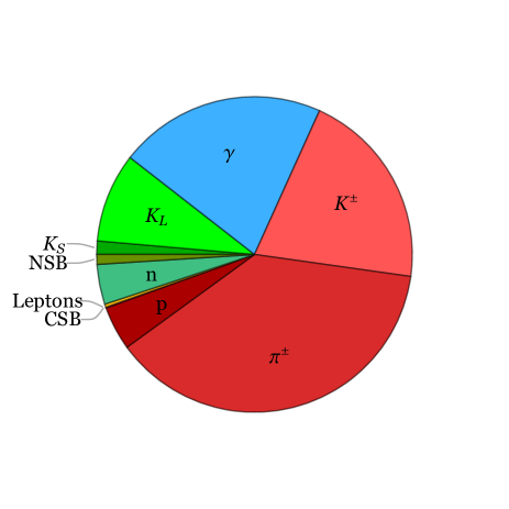
$~{}~{}~{}~{}~{}~{}~{}~{}~{}~{}~{}~{}~{}~{}~{}~{}{\rm Strange}~{}~{}p_{T}=45\,\rm GeV$

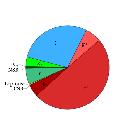
$~{}~{}~{}~{}~{}~{}~{}~{}~{}~{}~{}~{}~{}~{}~{}~{}{\rm Down}~{}~{}p_{T}=45\,\rm GeV$

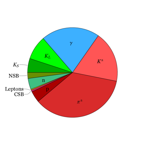
$~{}~{}~{}~{}~{}~{}~{}~{}~{}~{}~{}~{}~{}~{}~{}~{}{\rm Strange}~{}~{}p_{T}>200\,\rm GeV$

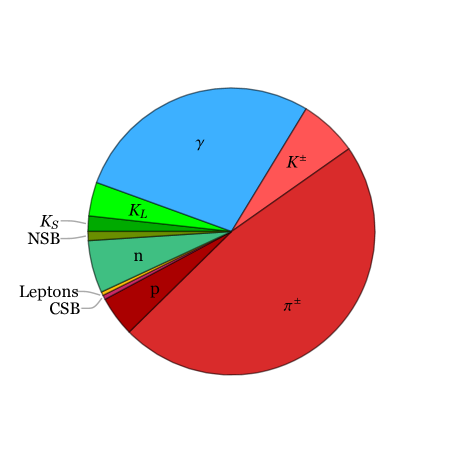
$~{}~{}~{}~{}~{}~{}~{}~{}~{}~{}~{}~{}~{}~{}~{}~{}{\rm Down}~{}~{}p_{T}>200\,\rm GeV$

Figure 1: Total momentum fractions carried by effectively detector stable particles that reach the calorimeters in strange- or down-quark jets arising from either $Z$-boson decay with central jet $p_{T}$ = 45 GeV, or from QCD initiated 13 TeV proton-proton central collisions with jet $p_{T}>200$ GeV, simulated with Pythia8. Here effectively detector stable is either a detector stable particle or a metastable particle that does not decay within a transverse distance of 150 cm from the beam line. Red and green correspond to electrically charged and neutral particles, and blue to photons. NSB and CSB refer to neutral and charged strange-baryons.

An important consideration in the practical utility of exploiting the differences between strange- and down-quark jets outlined above is the momentum fraction carried by the various types of detector stable and meta-stable particles within the jets. In order to visually illustrate these differences the truth-level average $p_{T}$ weighted momentum fractions obtained from Pythia8 for each type of effectively detector stable particle within the leading jet in the four sets of event samples described in the previous section are shown in the pie charts in Fig. 1. In this figure, effectively detector stable is defined to be a either detector stable particle or a meta-stable particle that does not decay within a transverse distance of 150 cm from the beam axis. Such particles reach and deposit energy in the calorimeters of the canonical general purpose collider detector considered here. All effectively detector stable particles within a jet that satisfy these criteria contribute to the momentum weighted fractions in the pie charts, including ones that originate directly from hadronization at the primary interaction vertex, as well as ones that emerge from secondary vertices from decays-in-flight of metastable particles. Red and green in the pie charts correspond to electrically charged and neutral particles respectively, and blue refers to photons.

A number of patterns evident in the pie charts in Fig. 1 are worth highlighting. In all cases for either strange- or down-quark jets, the momentum weighted fraction of charged kaons is twice that of long-lived neutral kaons. The is because the hadronization probability for charged and neutral kaons is essentially identical, and long-lived neutral kaons make up half of the neutral kaon content at hadronization. The charged kaons and long-lived neutral kaons are both detector stable particles and appear directly in the pie charts. In contrast, only a fraction of the short-lived neutral kaons that make up the other half of the neutral kaon content from hadronization reach the calorimeters at a transverse distance of 150 cm from the beam axis and appear in the pie charts, with the remainder undergoing decays-in-flight. The fraction of short-lived kaons that reach the calorimeters is directly proportional to the average lab-frame decay length, which in turn is proportional to the total transverse momentum of the jet. For $p_{T}=45$ GeV jets, the short-lived kaon momentum weighted fraction that reaches the calorimeters is rather small, while for $p_{T}>200$ GeV jets, it is a sizable fraction of that of the long-lived kaons. The momentum weighted fraction of neutral strange baryons that reaches the calorimeters for $p_{T}>200$ GeV jets is also larger than that for $p_{T}=45$ GeV jets for the same reason.

The charged kaon momentum weighted fractions in strange-quark jets shown in the pie charts on the left-hand side of Fig. 1 are more than three times larger than that in down-quark jets shown on the right-hand side. However, the sum of the charged kaon and charged pion momentum weighted fractions at hadronization are essentially identical. This is because the hadronization probability into charged particles for the net unit of strange-ness or down-ness within a strange- or down-quark jet respectively is roughly equal and dominated by these lightest net strange-ness and down-ness carrying mesons. The near equality of the sum of the charged kaon and charged pion momentum weighted fractions is evident in comparing the pie charts for strange- and down-quark jets with $p_{T}>200$ GeV in Fig. 1. For $p_{T}=45$ GeV the sum is slightly larger for strange-quark jets than for down-quark jets, with the excess coming mainly from decays-in-flight of short-lived neutral kaons to charged pion pairs. The current generation of general purpose collider detectors can not effectively distinguish charged kaons from charged pions. So the near equality of the sum of the momentum weighted fractions of these particles means that the individual differences can not be exploited as a handle to distinguish strange- and down-quark jets in these detectors.

The momentum weighted fraction of long-lived neutral kaons in strange-quark jets is more than two times larger than in down-quark jets. This is because a long-lived neutral kaon can carry the net unit of strange-ness in a strange-quark jet, but can not carry the net unit of down-ness in a down-quark jet. The difference is apparent in comparing the pie charts for strange- and down-quark jets with $p_{T}=45$ GeV as well as for $p_{T}>200$ GeV in Fig. 1. In a collider detector long-lived neutral kaons deposit energy primarily in the HCAL. So the excess fractional energy deposited there by the net unit of strangeness in a strange-quark jet provides an observable handle with which on average to distinguish these from down-quark jets. However, the momentum weighted neutron fraction is somewhat larger in down-quark jets than in strange-quark jets. This is because the net unit of down-ness in a down-quark jet can, with some small probability, be carried by a neutron. Since neutrons also deposit energy primarily in HCAL, this tends on average to reduce the effectiveness of neutral hadronic energy alone to distinguish strange-quark jets from down-quark jets.

The final important feature evident in the pie charts in Fig. 1 is that the photon momentum weighted fractions in strange-quark jets shown in the pie charts on the left are smaller than those in the down-quark jets shown on the right-hand side. Photons within both types of jets arise predominantly from prompt decays of neutral pions to photon pairs, and to a lesser extent from prompt eta and eta prime decays to photons, either directly or through cascade decays with intermediate neutral pions, and decays-in-flight of short-lived kaons to photons through intermediate neutral pion pairs. None of these states except the short-lived kaon carry net strangeness or down-ness. However, it is possible for the primary hard strange-quark to hadronize into one of these non-strangeness carrying states, with the net strange-ness or down-ness carried by a secondary state of lower momentum fraction. In a down-quark jet the probability that the primary down-quark from the hard process hadronizes into a charged pion is twice that into a neutral pion. In contrast, in a strange quark jet the only states that are available for the primary strange quark to hadronize into in conjunction with an up- or down-anti-quark are the strangeness carrying charged and neutral kaon mesons. The primary strange quark hardronizes into an eta meson only in conjunction with a heavier anti-strange-quark. So the primary hard quark in a strange-quark jet has lower probability to hadronize into a state that promptly decays to photons than in a down-quark jet. In strange-quark jets photons also arise from decays-in-flight of short-lived kaons, but the total momentum weighted photon fraction is still smaller than that of down-quark jets.

Although not of primary importance in distinguishing strange- and down-quark jets, it is also worth noting that the sum of the strange and non-strange baryon momentum weighted fraction in strange-quark jets is somewhat less than that in down-quark jets. This is because the larger mass of the strange-quark results in a smaller probability for strange-quarks to hadronize into strange baryons relative to mesons, compared with the probability for down-quarks to hadronize into non-strange baryons relative to mesons.

In summary, for effectively detector stable particles, the momentum weighted fraction of long-lived neutral kaons are higher in a strange-quark jet than in a down-quark jet. Conversely, the momentum weighted fraction of photons is smaller in a strange-quark jet than in a down-quark jet. And the total momentum weighted fraction in detector stable charged particles is very similar in both types of jets.

3.2 Strange and Down Jet Signatures in a Collider Detector

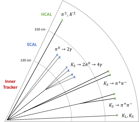
Figure 2: Cartoon (not to scale) of pions and kaons from central collisions traversing a transverse wedge of a general purpose high energy collider detector. Solid lines are charged particles, dashed lines are neutral particles, and dotted lines are photons. An $\times$ indicates that the particle is absorbed or stops within the calorimeter subsystem. Neutral pions decay promptly to photons that are absorbed in the electromagnetic calorimeter. Charged pions and kaons and long-lived neutral kaons are detector stable particles that are stopped in the hadronic calorimeter. Short-lived neutral kaons can decay in flight to neutral or charged pion pairs within any of the detector subsystems shown, or can be stopped before decay in the hadronic calorimeter.

The response of a general purpose collider detector to pions and kaons originating from the primary interaction point of a high energy collision are illustrated in Fig 2. The charged pion and kaon, $\pi^{-},K^{-}$, are both detector stable particles. The momenta of these particles are measured in the inner tracking region, and their energy is deposited primarily in the HCAL. These particles are essentially indistinguishable in the current generation of general purpose collider detectors. Neutral pions, $\pi^{0}$, decay promptly to photon pairs, $\pi^{0}\to\gamma\gamma$, that are absorbed in the ECAL. Long-lived neutral kaons are detector stable and deposit energy primarily in the HCAL. Short-lived neutral kaons can either reach the HCAL and deposit energy there before decaying, or undergo decays-in-flight to neutral or charged pion pairs. If such decays to neutral pions pairs, $K_{S}\to\pi^{0}\pi^{0}\to\gamma\gamma\gamma\gamma$, take place within the inner tracking region or ECAL, the resulting photons are absorbed in the ECAL. Decays of short-lived kaons to charged pion pairs within the ECAL, $K_{S}\to\pi^{+}\pi^{-}$, results in energy deposition mainly in the HCAL. For short-lived kaons that decay in-flight early enough within the inner tracking region to charged pions, $K_{S}\to\pi^{+}\pi^{-}$, the momenta can be reconstructed from the charged pions tracks which also deposit energy primarily in the HCAL.

The differences of the momentum weighted fractions of effectively detector stable particles in strange- and down-quark jets detailed in the previous sub-section, along with the detector responses to the most important of these particles outlined above, suggest three main (correlated) observables which can provide handles to distinguish between these types of jets. The first is the jet neutral hadronic energy fraction, $H_{N}$, defined in section 2. Since strange-quark jets have a higher momentum fraction of long-lived neutral kaons and short-lived kaons that reach the HCAL, this observable will on average be larger than for down-quark jets. The second is the jet electromagnetic neutral energy fraction, $E_{N}$. Since strange-quark jets have a lower momentum fraction of photons, this will on average be smaller than for down-quark jets. The third observable is the short-lived kaon $K_{S}\to\pi^{+}\pi^{-}$ decay-in-flight momentum fraction, $K_{S_{\pi^{+}\pi^{-}}}$, also defined in section 2. Since the neutral kaon momentum weighted fraction is larger for strange-quark jets, this observable will on average be larger than for down-quark jets. The remaining observable defined in section 2 is the charged track momentum fraction, $T$. As discussed in the previous sub-section, the charged particle momentum weighted fraction is not significantly different for strange- and down-quark jets. So this observable is not expected to add much discriminating power between these types of jets.

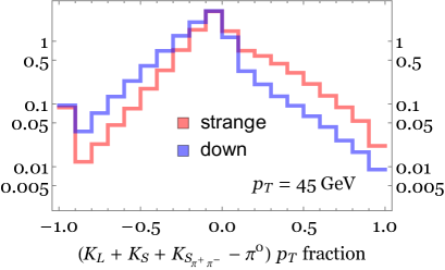
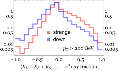
Figure 3: Pythia8 truth-level distributions (without detector simulation) of total neutral kaon minus neutral pion transverse momentum fraction for strange- (red) or down- (blue) quark central jets arising from either $Z$-boson decay or QCD initiated 13 TeV proton-proton collisions with jet $p_{T}>200$ GeV. Short-lived neutral kaons are only included with lab-frame decay distances greater than 150 cm or with decays to charged pion pairs with a lab-frame decay distance between 0.5 and 50 cm.

In order to gain a measure of the ultimate utility of these observables, it is instructive to first consider idealized truth-level jet variables without full detector effects. The change in the neutral kaon and photon momentum fractions shown in the pie charts in Fig. 1 are anti-correlated in going from strange-quark jets to down-quark jets. Since the photons arise mainly from neutral pion decay, a simple truth-level jet variable that captures this correlated difference is the neutral kaon momentum fraction minus the neutral pion momentum fraction. The distributions of this truth-level variable obtained from Pythia8 for the leading jet in each event in the four sets of event samples described in section 2 are shown in Fig. 3. In order to retain some of the most relevant irreducible detector effects, only short-lived neutral kaons that reach the HCAL at 150 cm from the beam axis, or decay to charged pion pairs in the inner tracking region with lab-frame decay distance between 0.5 and 50 cm (and so can be reconstructed in the inner tracking region) are included in Fig. 3. All neutral pions and long-lived neutral kaons are included. Although in all cases the distributions peak at similar values of the neutral kaon minus neutral pion momentum fraction, the distributions for strange-quark jets are shifted to larger values, with the largest fractional differences in the tails of the distributions at large and small values.

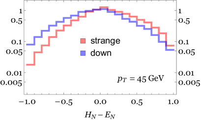
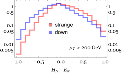
Figure 4: Distribution of jet total neutral hadronic energy fraction, $H_{N}$, minus total electromagnetic energy fraction, $E_{N}$, from the Delphes detector simulation for strange (red) or down (blue) quark central jets arising from either $Z$-boson decay or QCD initiated 13 TeV proton-proton central collisions with jet $p_{T}>200$ GeV.

The detector-level observable version of the neutral kaon minus neutral pion momentum fraction is the neutral hadronic energy minus neutral electromagnetic energy of a jet, $H_{N}-E_{N}$. The distributions of this detector-level variable obtained from Delphes for the leading jet in each event in the four sets of event samples described in section 2 are shown in Fig. 4. Although somewhat washed out compared with the distributions of the truth-level variable given above, the same general features are still apparent, with strange-quark jet distributions shifted to higher values compared with down-quark jets.

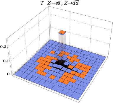
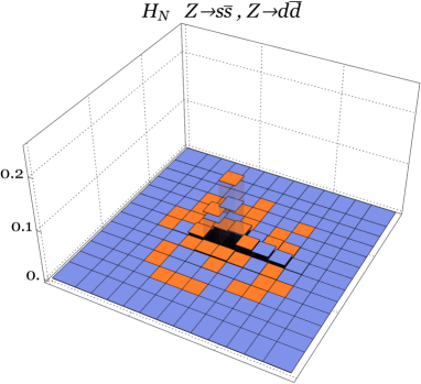
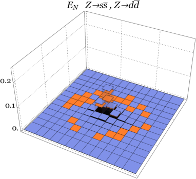
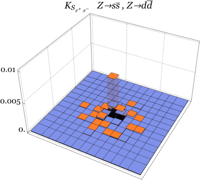
Figure 5: Average jet lego plot images from Delphes detector simulation of charged track transverse momentum fraction, $T$, hadronic neutral energy fraction, $H_{N}$, electromagnetic energy fraction, $E_{N}$, and momentum fraction of short-lived kaons that decay to charged pion pairs with lab-frame decay length between 0.5 and 50 cm, $K_{S_{\pi^{+}\pi^{-}}}$, for strange- (orange) and down- (blue) quark jets arising from $Z$-boson decay. The lego plots cover a total area of 1.2 $\times$ 1.2 in the $\eta-\phi$ plane with pixel size $0.1\times 0.1$. Each jet image within the average is centered and rotated.

A more refined picture of the observable differences between strange- and down-quark jets can be gleaned from the distributions of detector-level observables in the plane transverse to the jet direction. Lego plots of the jet averaged charged track momentum fraction, neutral hadronic and neutral electromagnetic energy fractions, and $K_{S}\to\pi^{+}\pi^{-}$ momentum fraction, $T,H_{N},E_{N},K_{S_{\pi^{+}\pi^{-}}}$, over the $\eta-\phi$ plane obtained from Delphes for the leading jet in the $p_{T}=45$ GeV event samples from $Z$-boson decay are shown in Fig. 5. Orange legos correspond to strange-quark jets, and blue to down-quark jets. The lego images cover a total area of $1.2\times 1.2$ in the $\eta-\phi$ plane, with pixel of size of $0.1\times 0.1$. The charged track momentum fractions are summed over individual charged tracks within each pixel, and the neutral energy fractions are summed over the appropriate calorimeter towers with centers that lie within each pixel. Following the jet preprocessing procedure used in previous studies [42] each individual jet image is shifted, rotated, and flipped so that the centroid of $T+E_{N}+H_{N}$ coincides with the central pixel, the principal axis is in the vertical direction, and the maximum intensity is in the upper right region.

A number of observable differences between strange-quark and down-quark jets are apparent in the lego images in Fig. 5. The average neutral hadronic energy fraction is larger for strange-quark jets, and conversely the average neutral electromagnetic energy fraction is larger for down-quark jets, consistent with the pie charts in Fig. 1. Most importantly though, these differences are localized mainly in the highest intensity central pixel at the centroid of the jets. The next highest intensity pixel to the left of central pixel in the images, shows a somewhat reduced difference for these observables, with even smaller differences in the remaining pixels. This arises because after QCD showering the primary hard quark can carry a significant fraction of the jet total momentum, and therefore by definition be near the centroid of the jet. For a primary hard strange-quark that hadronizes in a long-lived neutral kaon, the resulting excess neutral hadronic energy then tends to be localized near the centroid of the jet. Likewise, for a primary hard down-quark that hadronizes in a neutral pion that then promptly decays to photon pairs, the resulting excess neutral electromagnetic energy tends to be localized near the centroid of the jet. So the greatest power of neutral hadronic and neutral electomagnetic energy fraction to discriminate strange- and down-quark jets is expected to come from the central region of jets.

Another striking difference between strange- and down-quark jets that is apparent in the lego images in Fig. 5 is the larger momentum fraction for strange-quark jets with $K_{S}\to\pi^{+}\pi^{-}$ decays that can be reconstructed. Just as for the neutral hadronic energy fraction, this excess momentum fraction tends to be localized near the centroid of the jets. This difference is more pronounced than that in the neutral hadronic or neutral electromagnetic energy fractions near the centroid of the jets because reconstructing the leading short-lived kaon with in-flight decay $K_{S}\to\pi^{+}\pi^{-}$ isolates a single strangeness carrying particle, which in a strange-quark jet has a good probability of containing the primary hard strange-quark with the net unit of strangeness within the jet. However, because of the branching ratio and very conservative reconstruction efficiency assumed here, only 8% of strange-quark jets and 5% of down-quark jets have such reconstructed decays-in-flight. Even so, for those strange-quark jets with a reconstructed $K_{S}\to\pi^{+}\pi^{-}$ near the centroid of the jet, this observable provides better discrimination from down-quark jets than does the neutral hadronic or neutral electromagnetic energy fractions near the centroid.

Finally, it is worth noting that the charged track momentum fractions for strange- and down-quark jets in Fig. 5 are very similar on average everywhere in the transverse plane of the jets. This is because, as described in section 3.1, the probability for a down-quark to hadronize in a charged pion is very similar to the probability for a strange-quark to hadronize in a charged kaon.

The important features of the lego images for strange- and down-quark jets obtained from Delphes for the leading jet in the $p_{T}>200$ GeV event samples are very similar to those outlined above, except that the overall intensity of the $K_{S}\to\pi^{+}\pi^{-}$ momentum fraction is smaller in both cases. For larger jet total momentum a higher fraction of the short-lived kaons reach the HCAL before decaying, resulting in relatively fewer decays-in-flight.

4 Strange Versus Down Jet Tagging Algorithms

Some of the detector-level observables presented in the previous section show clear differences between strange- and down-quark jets. In this section we describe a number of different tagging algorithms that exploit these detector-level differences as handles to on average distinguish between strange- and down-quark jets. The algorithms range from simple cuts on single whole-jet variables, BDTs with a few whole-jet variables, to deep learning CNNs with appropriately chosen multi-color jet images. The algorithms and their input sources and variables are listed in Table 1. Results and comparisons of the performance of the algorithms are presented in section 5.

Algorithm	Input Source	Input Variable(s)
Cut1	Delphes	$H_{N}-E_{N}$
Cut1+	Delphes	$H_{N}-E_{N}+K_{S_{\pi^{+}\pi^{-}}}$
BDT3	Delphes	$H_{N}\,,\,E_{N}\,,\,T$
BDT4	Delphes	$H_{N}\,,\,E_{N}\,,\,T\,,\,K_{S_{\pi^{+}\pi^{-}}}$
CNN3	Delphes	$H_{N}\,,\,E_{N}\,,\,T$              13$\times$13 Jet Image
CNN4	Delphes	$H_{N}\,,\,E_{N}\,,\,T\,,\,K_{S_{\pi^{+}\pi^{-}}}$  13$\times$13 Jet Image
Truth Cut1	Pythia8	$-\pi^{0}+K_{L}+K_{S}+K_{S_{\pi^{+}\pi^{-}}}$
Truth BDT3	Pythia8	$\pi^{0}\,,\,K_{L}\,,\,K_{S}+K_{S_{\pi^{+}\pi^{-}}}$

Table 1: Strange versus down jet tagging algorithms input source and variable(s) utilized in this work. Pythia8 truth-level variables $\pi^{0}$ and $K_{L}$ are jet total momentum fractions in neutral pions and long-lived neutral kaons respectively, $K_{S}$ is total momentum fraction for short-lived neutral kaons that decay with a lab-frame distance greater than 150 cm, and $K_{S_{\pi^{+}\pi^{-}}}$ is total momentum fraction for short-lived neutral kaons that decay to charged pion pairs with a lab-frame distance between 0.5 and 50 cm. Delphes variable $H_{N}$ is jet neutral hadronic energy fraction, $E_{N}$ is electromagnetic energy fraction, $T$ is track momentum fraction, and $K_{S_{\pi^{+}\pi^{-}}}$ is as defined above. Delphes variables for Cut and BDT algorithms are for the entire jet. For CNN algorithms the Delphes variables are defined over a centered and rotated 13$\times$13 jet image that covers 1.2$\times$1.2 in the $\eta\!-\!\phi$ plane.

4.1 Single Variable Cut-Based and Multi-Variable BDT Classifiers

The simplest possible classifier for distinguishing strange-quark from down-quark jets is a simple cut on a single whole-jet detector based variable. As discussed in section 3.2, in going from a strange-quark jet to a down-quark jet, the neutral energy fraction, $H_{N}$, and neutral electromagnetic energy fraction, $E_{N}$, are anti-correlated. So $H_{N}-E_{N}$ is a very simple whole-jet variable that should provide some discrimination, which we refer to as Cut1. The momentum fraction $K_{S_{\pi^{+}\pi^{-}}}$ of short-lived kaons with reconstructed decays-in-flight to charged pion pairs, $K_{S}\to\pi^{+}\pi^{-}$, provides additional discriminating power. So we also use the whole-jet combination $H_{N}-E_{N}+K_{S_{\pi^{+}\pi^{-}}}$, which we refer to as Cut1+. We have also considered other linear combinations of the four observables discussed in section 3.2, $H_{N},E_{N},T,K_{S_{\pi^{+}\pi^{-}}}$, but Cut1 and Cut1+ give the best single variable discriminating power at the whole-jet level.

In order to account for correlations among the four detector-level observables listed above, we utilize a BDT algorithm with whole-jet inputs of either $H_{N},E_{N},T$ or $H_{N},E_{N},T,K_{S_{\pi^{+}\pi^{-}}}$, which we refer to as BDT3 and BDT4 respectively. The BDT networks are trained to distinguish between strange- and down-quark jets with either the $p_{T}=45$ GeV or $p_{T}>200$ GeV event samples described in section 2. The algorithms are tested on independent event samples, with the BDT output used as a single classifier variable on which to cut.

It is instructive to compare these detector-level whole-jet classifiers with classifiers based on analogous truth-level whole-jet information. For a single truth-level variable we employ the whole-jet neutral kaon momentum fraction minus the neutral pion momentum fraction discussed in section 3.2. To retain some irreducible detector level effects, only short-lived kaons that reach the HCAL at 150 cm from the beam axis, or decay to charged pion pairs with a lab-frame distance between 0.5 and 50 cm are included. We refer to this classifier as Truth Cut1. For a classifier that accounts for correlations among truth-level variables we utilize a BDT algorithm with whole-jet inputs of the neutral pion momentum fraction, the long-lived neutral kaon momentum fraction, and the short-lived neutral kaon momentum fraction with the restrictions above. We refer to this classifier as Truth BDT3. We view this classifier as roughly setting the maximal performance that can be achieved for discriminating strange-quark from down-quark jets with whole-jet variables, given some of the irreducible detector-level effects of the current generation of general purpose collider detectors.

4.2 Deep Learning CNN-Based Jet Image Classifiers

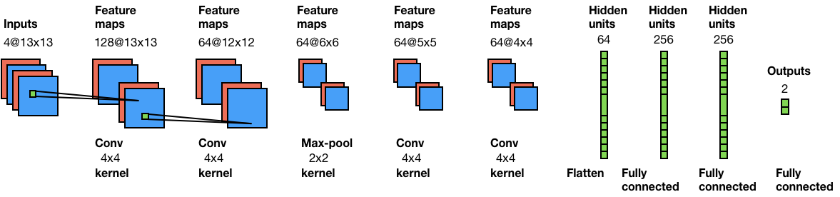
Figure 6: The deep learning convolutional neural network architecture CNN4 utilized here for discriminating strange-quark and down-quark jets. The inputs are 13$\times$13 jet images from the Delphes detector simulation covering a total area of 1.2$\times$1.2 in the $\eta\!-\!\phi$ plane with 4 colors corresponding to the normalized variables $H_{N},E_{N},T,K_{S_{\pi^{+}\pi^{-}}}$ in each pixel. The CNN3 architecture is identical with 3 colors corresponding to $H_{N},E_{N},T$ in each pixel. The images are centered and rotated. Two outputs correspond to strange-quark or down-quark jet.

Going beyond whole-jet variables, a more detailed picture of the differences between strange- and down-quark jets is provided by the distribution of detector-level observables in the plane transverse to the jet direction, as discussed in section 3.2. In order to capture these finer details we use a CNN algorithm with pixelated multi-color jet image inputs of either the detector-level observables $H_{N},E_{N},T$ or $H_{N},E_{N},T,K_{S_{\pi^{+}\pi^{-}}}$, which we refer to as CNN3 and CNN4 respectively. The jet image inputs for each of these detector-level observables correspond precisely to those shown in Fig. 5, with $13\times 13$ pixels of size $0.1\times 0.1$ in the $\eta-\phi$ plane with the same preprocessing described in section 3.2.

The architecture of the CNN algorithm we utilize is shown in Fig. 6, and is a variation of one used in previous studies [42]. The 3 or 4 input images from each jet enter the first convolutional layer of 128 filters through a local $4\times 4$ kernel. The generated 128 feature maps are then coupled to the next convolutional layer of 64 filters with another local $4\times 4$ kernel. This is followed by a max-pooling layer with a $2\times 2$ reduction factor. The resulting 64 feature maps are coupled sequentially through two more convolutional layers, each of which has 64 filters with a local $4\times 4$ kernel. These 64 feature maps are then coupled directly through three sequential fully-connected layers with 64, 256 and 256 neurons respectively. Finally, the output layer has two neurons corresponding to strange- or down-quark jets. A softmax function is used as activation to output the classification probabilities. All the convolutional layers and fully-connected layers in the CNN have Rectified Linear Units (ReLUs) as activation. The CNNs are trained to distinguish between strange- and down-quark jets with either the $p_{T}=45$ GeV or $p_{T}>200$ GeV event samples described in section 2. Independent event samples are employed for training and testing. We use cross entropy for the loss function and Adadelta [43] for the optimizer. The CNN output is used as a single classifier variable on which to cut.

We have also tried Adam [44] for the CNN optimizer but the classification results do not show any improvement. In addition, we have changed the number of filters or added another max-pooling layer just before the fully-connected layers, again with no significant improvement. Finally, we have tried ResNet algorithms along the lines of another previous study [45] but they did not offer superior performance over the CNN architecture.

5 Strange Versus Down Jet Tagging Algorithms Performance

All of the algorithms outlined in the last section provide some level of discrimination between strange- and down-quark jets. In the first sub-section below, the training sample sizes required for the BDT and CNN algorithms are discussed. In the next sub-section the relative and absolute performance of all the algorithms are compared. In the final sub-section the correlation between the classifier output of one of the CNN algorithms and the long-lived kaon momentum fraction is investigated.

5.1 Training Sample Size for BDT and CNN Algorithms

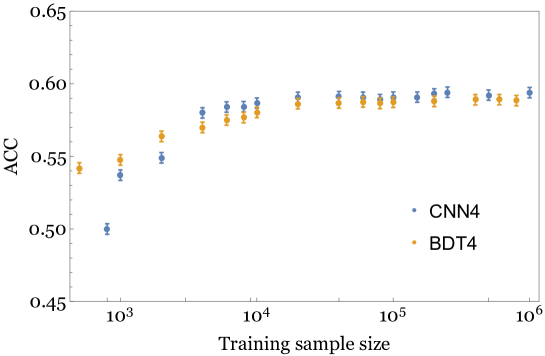
Figure 7: Classification accuracy of strange-quark versus down-quark central jets from $Z$-boson decay for the BDT4 (orange) and CNN4 (blue) strange jet tagging algorithms, as a function of the training sample size for a fixed independent testing sample of $10^{4}+10^{4}$ strange plus down jets. Error bars correspond to binomial statistical standard deviation of the testing sample. The BDT4 and CNN4 tagging algorithm inputs are given in Table 1.

The BDT and CNN algorithms are trained to distinguish between strange- and down-quark jets with either the $p_{T}=45$ GeV or $p_{T}>200$ GeV event samples described in section 2. An important figure of merit for these algorithms is the number of training events required to obtain good performance. As an overall measure of the performance for a given number of training events, we use the best accuracy, ACC, defined to be the average of the true positive and true negative rate, maximized over all values of the classifier output variable. The best accuracy for the BDT4 and CNN4 algorithms are shown in Fig. 7 as a function of the training event sample size for the $p_{T}=45$ GeV event samples from $Z$-boson decay. For both algorithms the performance saturates with more than roughly $10^{4}$ training events. By contrast, at least 10 times more training events were needed in a previous study to saturate performance for boosted hadronic top-quark tagging [42]. This is perhaps not surprising since boosted hadronic top-quark jets have more localized substructure in the plane transverse to the jet direction than do strange- and down-quark jets.

5.2 Comparison of Strange Jet Tagging Algorithms

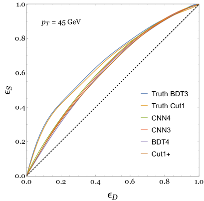
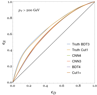
Figure 8: Strange jet tagging algorithm ROC curves for the fraction of strange-quark central jets correctly tagged as strange jets, $\epsilon_{S}$, as a function of the fraction of down-quark central jets incorrectly tagged as strange jets, $\epsilon_{D}$, arising from either $Z$-boson decay or QCD initiated 13 TeV proton-proton collisions with jet $p_{T}>200$ GeV. Tagging algorithm inputs are given in Table 1. The dashed diagonal line corresponds to random tagging of strange- versus down-quark jets.

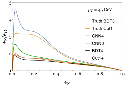
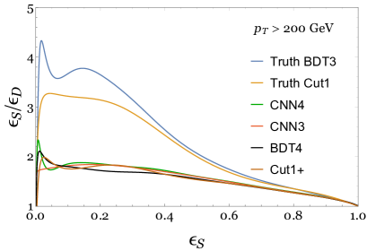
Figure 9: The ratio of strange-quark to down-quark central jets tagged as strange jets, $\epsilon_{S}/\epsilon_{D}$, as a function of the fraction of strange-quark jets tagged as strange jets, $\epsilon_{S}$, arising from either $Z$-boson decay or QCD initiated 13 TeV proton-proton collisions with jet $p_{T}>200$ GeV. The tagging algorithm inputs are given in Table 1.

All the strange- versus down-quark tagging algorithms presented in section 4 output a single classifier variable. Jets within events in a testing set with classifier values larger than a threshold or cut value may be tagged as strange-quark like jets. With this prescription, it is convenient to define the tagging rate, $\epsilon_{S}$, to be the fraction of strange-quark jets in a testing sample set that are tagged as strange-quark like jets, and the mistag rate, $\epsilon_{D}$, to be the fraction of down-quark jets in a testing sample set that are tagged as strange-quark like jets. The Receiver Operating Characteristic (ROC) curve for a tagging algorithm is then defined as the pair $\epsilon_{S},\epsilon_{D}$ as a function of the classifier cut value.

The ROC curves for the whole-jet detector-level algorithms Cut1+ and BDT4, the whole-jet truth-level algorithms Truth Cut1 and Truth BDT3, and the detector-level jet image algorithms CNN3 and CNN4 are shown in Fig. 8 for both the $p_{T}=45$ GeV and $p_{T}>200$ GeV event samples described in section 2. For comparison, a random tagging of strange- versus down-quark jets would yield a diagonal ROC curve. The truth-level whole-jet algorithms have better performance than any of the detector-level algorithms for nearly all classifier cut values. This indicates that the detector-level observables tend to wash out the information in the more idealized truth-level variables. Of particular importance in this regard, the discriminating power from the larger momentum weighted fraction of long- and short-lived neutral kaons that reach the HCAL in strange-quark jets is partially overcome by the larger momentum weighted fraction of neutrons in down-quark jets, as discussed in section 3.1.

In order to better expose the differences between the strange-quark jet tagging algorithms, ratio ROC curves, defined as the pair $\epsilon_{S}/\epsilon_{D},\epsilon_{S}$ as a function of the classifier cut value, are shown in Fig. 9. For the $p_{T}=45$ GeV jet event samples from $Z$-boson decay, among the algorithms based on detector-level observables, CNN4 with jet image inputs shows the best discrimination between strange- and down-quark jets for all classifier cut values. It is better than the whole-jet BDT4 algorithm with the same detector-level inputs integrated over the plane transverse to the jet direction. As discussed in section 3.2, the differences between strange- and down-quark jets in hadronic neutral energy, electromagnetic neutral energy, and short-lived kaon $K_{S}\to\pi^{+}\pi^{-}$ reconstructed momenta, are localized mainly near the centers of jets. The spatial distribution of these detector-level observables in the transverse plane is available to the CNN4 algorithm, but not the BDT4 algorithm.

The CNN3 algorithm with detector-level inputs is essentially identical in architecture to the CNN4 algorithm, except that it doesn’t include the momentum fraction of reconstructed short-lived kaon decays-in-flight to charged pion pairs, $K_{S}\to\pi^{+}\pi^{-}$. This accounts for the better performance of CNN4 compared with CNN3 for the $p_{T}=45$ GeV jet event samples shown in Fig. 9. The difference in performance is more pronounced for smaller values of the strange-quark jet tagging rate, $\epsilon_{S}$. As discussed in section 3.2, because of the branching ratio and very conservative reconstruction efficiency only 8% of strange-quark jets in this event sample have reconstructed $K_{S}\to\pi^{+}\pi^{-}$ decays-in-flight. For smaller values of the strange-quark jet tagging rate, obtained for harder cuts on the classifier output variable, the CNN4 algorithm makes effective use of the somewhat rare reconstructed $K_{S}\to\pi^{+}\pi^{-}$ decays-in-flight. With this additional discriminating handle, the CNN4 algorithm obtains peak performance of $\epsilon_{S}/\epsilon_{D}\simeq 2.5$ in distinguishing strange- and down-quark jets in this event sample at the somewhat small value of strange-quark tagging rate of $\epsilon_{S}\simeq 0.02$.

The whole-jet truth-level Truth BDT3 algorithm has better performance than the whole-jet single variable truth-level Truth Cut1 algorithm for all values of the classifier variable cut. The difference is more pronounced for smaller values of the strange-quark jet tagging rate. Just as above, this arises mainly from the reconstructed $K_{S}\to\pi^{+}\pi^{-}$ decays-in-flight. The whole-jet Truth BDT3 algorithm makes use of these somewhat rare reconstructed decays-in-flight at small values of the strange-quark jet tagging rate. The occurrence of such decays-in-flight is infrequent enough that the information about the spatial distribution is less important than for other observables. In contrast, for Truth Cut1 the contribution of the momentum fraction of these decays-in-flight to the single whole-jet variable of this algorithm is diluted. The whole-jet detector-level BDT4 algorithm also makes use of the reconstructed $K_{S}\to\pi^{+}\pi^{-}$ decays-in-flight to obtain better performance at small values of the strange-quark jet tagging rate.

The detector-level whole-jet algorithms BDT4 and Cut1+ and jet image algorithms CNN3 and CNN4 all have somewhat similar performance for nearly all classifier cut values for the $p_{T}>200$ GeV jet event samples shown in Fig. 9. This is unlike the $p_{T}=45$ GeV jet samples for which the CNN4 jet image algorithm has noticeably better performance than the other detector-level algorithms for small classifier cut values. As discussed in section 3.1, the main observable difference between these jet samples is that for $p_{T}>200$ GeV a sizable fraction of the short-lived neutral kaons reach the HCAL and deposit energy there. This leaves a smaller fraction of short-lived neutral kaons with decays-in-flight to charged pion pairs, $K_{S}\to\pi^{+}\pi^{-}$, that can be reconstructed for $p_{T}>200$ GeV jets. The primary observable handle available to distinguish strange- from down-quark jets that remains is then the hadronic neutral and electromagnetic neutral energy fractions, with all the detector-level algorithms giving somewhat similar performance. However, at very small values of classifier cut values, the CNN4 and BDT4 algorithms as well as Cut1+ that all include the reconstructed $K_{S}\to\pi^{+}\pi^{-}$ momentum fraction, do show some improvement in performance compared with the CNN3 algorithm that does not include this information. All of this illustrates the added benefit of including reconstructed decays-in-flight of short-lived kaons to charged pion pairs, $K_{S}\to\pi^{+}\pi^{-}$, in strange-quark jet tagging, particularly for lower momentum jets.

	AUC	ACC	R10	R50
Truth Cut1	0.65 (0.68)	0.61 (0.62)	31.9 (32.1)	3.6 (3.9)
Truth BDT3	0.67 (0.68)	0.62 (0.62)	37.3 (37.1)	3.7 (4.0)
Cut1	0.61 (0.63)	0.57 (0.59)	16.4 (17.9)	2.7 (3.0)
Cut1+	0.62 (0.63)	0.58 (0.60)	17.9 (18.8)	2.9 (3.1)
BDT3	0.61 (0.63)	0.59 (0.60)	16.0 (17.1)	2.9 (3.1)
BDT4	0.63 (0.63)	0.60 (0.60)	22.5 (16.6)	3.2 (3.2)
CNN3	0.62 (0.63)	0.59 (0.60)	17.9 (18.4)	3.0 (3.2)
CNN4	0.64 (0.64)	0.60 (0.60)	23.9 (18.8)	3.3 (3.2)

Table 2: Area under ROC curve, accuracy, and rejection factors R10 = $1/\epsilon_{D}$ for $\epsilon_{S}=0.1$, and R50 = $1/\epsilon_{D}$ for $\epsilon_{S}=0.5$, for various strange jet tagging algorithms applied to Monte Carlo samples with equal numbers of strange-quark and down-quark jets. Numbers without parentheses are for strange- and down-quark central jets from $Z$-boson decay, and with parentheses likewise from QCD initiated 13 TeV proton-proton collisions with jet $p_{T}>200$ GeV.

Numerical measures of the performance of all the strange- versus down-quark jet tagging algorithms listed in Table 1 are presented in Table 2 for both the $p_{T}=45$ GeV and $p_{T}>200$ GeV event samples described in section 2. Among the detector-level algorithms, the CNN4 algorithm with jet image inputs has the best performance. The area under the ROC curve, AUC, for this algorithm is 0.64 for both event samples. For comparison, a perfect tagging algorithm would have AUC equal to 1.0 and a random algorithm would have 0.5. The accuracy, ACC defined in section 5.1, for this algorithm is 0.60. The down-quark jet rejection factor for the CNN4 algorithm, defined to be $1/\epsilon_{D}$, reaches a value of 23.9 for $\epsilon_{S}=0.1$, corresponding to $\epsilon_{S}/\epsilon_{D}=2.39$, for the $p_{T}=45$ GeV event sample.

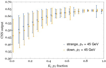
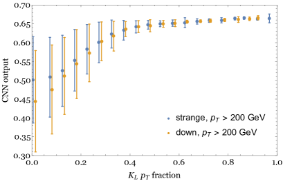
Figure 10: CNN3 classifier variable output as a function of Pythia8 truth-level long-lived kaon transverse momentum fraction for strange- or down-quark central jets arising from either $Z$-boson decay or QCD initiated 13 TeV proton-proton collisions with jet $p_{T}>200$ GeV. The CNN3 inputs are given in Table 1. The training and independent testing samples are $10^{6}+10^{6}$ and $10^{5}+10^{5}$ events respectively of strange- plus down-quark jets. The central dot in each bin corresponds to the average CNN3 classifier variable output, and the error bar corresponds to the variance in each bin.

5.3 Correlation of CNN3 Algorithm with Long-Lived Kaon Momentum Fraction

In a general purpose high energy collider detector, the primary observable differences between strange- and down-quark jets are for the momentum fraction of neutral kaons with a concomitant anti-correlated momentum fraction of neutral pions, as detailed in section 3. In order to assess quantitatively the extent to which a detector-level strange-quark jet tagging algorithm is exploiting these primary physical differences, it is useful to look at the correlation between the classifier output variable and the neutral kaon momentum fraction. To expose this correlation it is most instructive to consider the CNN3 algorithm with detector-level jet image inputs of only the hadronic neutral and electromagnetic neutral energy fractions, and the track momentum fraction, $H_{N},E_{N},T$. This algorithm does not include reconstructed decays-in-flight of short-lived neutral kaons, so the relevant neutral kaon momentum fraction with which to compare is that of the long-lived neutral kaons that reach the HCAL and contribute to the $H_{N}$ detector-level observable.

The average value and variance of the classifier output variable for the CNN3 algorithm for strange- and down-quark jets in both the $p_{T}=45$ GeV and $p_{T}>200$ GeV event samples are shown in Fig. 10 in bins of the truth-level long-lived neutral kaon momentum fraction (anomalously large variance results in a few cases because of low statistics). There is a clear correlation between the classifier output variable and the long-lived neutral kaon momentum fraction, with a smaller variance for larger values of the momentum fraction. At large values of the long-lived neutral kaon momentum, the classifier output variable saturates to a unique value (with very small variance) that depends only on the jet transverse momentum. The correlation and saturation occurs for both the strange- and down-quark jet samples. This indicates that, through the network training, the CNN3 algorithm has learned to classify a jet as strange-quark like based largely on the long-lived neutral kaon momentum fraction, particularly when it is large.

For smaller values of the long-lived neutral kaon momentum fraction the average value of the CNN3 classifier output variable shown in Fig. 10 is different for strange- and down-quark jets, but with a large variance. This indicates that the CNN3 algorithm has learned to use other information to distinguish strange- from down-quark jets when the long-lived neutral momentum fraction is small. For these cases there is a good probability that another type of particle carries the net unit of strange-ness in a strange-quark jet, such as a short-lived neutral kaon that reaches the HCAL and contributes to the $H_{N}$ detector-level observable, or a short-lived kaon that decays-in-flight to a pair of either neutral or charged pions that can contribute to the $E_{N}$ or $T$ detector-level observables respectively, depending on the lab-frame decay distance. This is also why the CNN3 classifier output variable saturates in the $p_{T}>200$ GeV jet samples for smaller values of the long-lived neutral kaon momentum fraction than in the $p_{T}=45$ GeV jet samples. In the former case, more short-lived neutral kaons reach the HCAL and contribute to the $H_{N}$ detector-level variable than in the latter case, as discussed in section 3.1.

6 Possible Application of Strange-Quark Jet Tagging

The ultimate utility of any object reconstruction and tagging algorithm is its deployment in the analysis of data from a high energy collider detector. In the first two sub-sections below, the statistical improvement obtained from a general binary tagging algorithm in a new physics search, or measurement of known process, is presented. In the final sub-section we discuss the decay of a $W$-boson to a charm-quark and either a strange- or down-quark, as a high purity source of strange-quark jets.

6.1 Improvements to New Physics Searches from Tagging Algorithms

The classifier output variable from a tagging algorithm may be treated like any other variable in an analysis of high energy collider data. For a binary tagging algorithm, two categories at either an object or event level may be formed based on whether the classifier output variable is larger or smaller than some cut or threshold value. The resulting categories can be integrated in to and improve an analysis.

In order to assess the impact of using the classifier output variable from a tagging algorithm, consider first a search for a new physics process in some region of the data from a high energy collider detector that, without use of the tagging algorithm, yields $S$ signal events and $B$ background events. Neglecting any systematic uncertainty in the expected number of background events, and in the limit $1\ll S\ll B$ considered for simplicity here and below in this sub-section, the event count statistical significance for a search limit or discovery without the tagging algorithm is ${\cal S}\simeq S/\sqrt{B}$.

In theory-level studies of the impact of tagging algorithms on new physics searches, it is common to simply throw away events with classifier output variables smaller than some cut value, and only keep the remaining events in the analysis. In this case a fraction $\epsilon_{S}$ of the signal events, and a fraction $\epsilon_{B}$ of the background events, remain after the classifier value cut. With this prescription, the resulting event count statistical significance for a search limit or discovery is

$${\cal S}_{\rm cut}\simeq{\epsilon_{S}\over\sqrt{\epsilon_{B}}}\,{S\over\sqrt{B}}$$ (6.1)

In the theory literature the quantity ${\cal S}_{\rm cut}/{\cal S}=\epsilon_{S}/\sqrt{\epsilon_{B}}$ is often referred to as the statistical significance improvement. Note that this simple cut based implementation of a tagging algorithm with a single category, may or may not provide an improvement in the statistical significance depending on whether or not the working point defined by the pair $\epsilon_{S},\epsilon_{B}$, that results from a given value of the classifier cut variable, yields a significance improvement factor greater or less than unity respectively.

In a modern analysis of actual collider detector data, it has become standard to bin rather than cut in any number of variables, including tagging algorithm classifier variables. With a binary tagging algorithm, binning makes use of both tagging categories, and by definition improves the sensitivity. A fraction $\epsilon_{S}$ of the signal events, and $\epsilon_{B}$ of the background events form one category, and a fraction $1-\epsilon_{S}$ of the signal events and $1-\epsilon_{B}$ of the background events form a second category. With this, the event count combined statistical significance for a search limit or discovery is the quadrature sum of the statistical significances of the two categories

$$\begin{split}{\cal S}_{\rm bin}\simeq\sqrt{\bigg{(}{\epsilon_{S}\over\sqrt{\epsilon_{B}}}{S\over\sqrt{B}}\bigg{)}^{2}+\bigg{(}{(1-\epsilon_{S})\over\sqrt{(1-\epsilon_{B})}}{S\over\sqrt{B}}\bigg{)}^{2}}=\sqrt{1+{(\epsilon_{S}-\epsilon_{B})^{2}\over\epsilon_{B}(1-\epsilon_{B})}}\,{S\over\sqrt{B}}\end{split}$$ (6.2)

For any binary tagging algorithm working point defined by the pair $\epsilon_{S},\epsilon_{B}$ this two category event count statistical significance is greater than that obtained from the single category cut based approach, or from that without use of the tagging algorithm. Ignoring any issues of systematic uncertainties, it is always better to bin rather than cut, or to not bin at all.

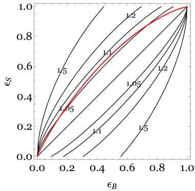
Figure 11: Contours of the event count combined statistical significance improvement provided by a two-category event-level tagging algorithm as a function of signal and background tagging efficiencies $\epsilon_{S},\epsilon_{B}$. For reference, the ROC curve for the CNN4 strange- versus down-quark jet tagging algorithm for the $p_{T}=45$ GeV jet event samples is overlaid in red.

The binned event count statistical significance improvement, ${\cal S}_{\rm bin}/{\cal S}$, is a useful figure of merit for the improvement provided by a binary tagging algorithm. Contours of this improvement factor are shown in Fig. 11 as a function of $\epsilon_{S},\epsilon_{B}$ for a general event-level binary tagging algorithm. For reference, the ROC curve for the CNN4 strange- versus down-quark jet tagging algorithm shown in Fig. 8 for the $p_{T}=45$ GeV events samples is overlaid in Fig. 11. This illustrates the statistical event count significance improvement that could be achieved with a binned two-category strange- versus down-quark CNN4 tagging algorithm in a hypothetical new physics search with signal events that include only a single strange-quark jet, with a much larger number of analogous background events that include only a single down-quark jet. For such an idealized new physics search, the CNN4 tagging algorithm could provide a modest 5% improvement in the event count statistical significance over a wide range of classifier category values.

6.2 Measurements with Tagging Algorithms

Tagging algorithms can also be useful in measurements of known processes at high energy colliders. Just as for a new physics search, with a binary tagging algorithm, two categories at either the object or event level may be formed based on a classifier output value. The discriminating power this offers can improve a measurement or even make feasible a measurement that was otherwise not possible.

In order to illustrate the use of a tagging algorithm in a measurement of some known physics process, consider a region of the data from a high energy collider detector with $S$ events of one type and $B$ events of a second type. A binary tagging algorithm designed to distinguish these two types of events may be used to form two categories of events based on a cut or threshold value of the output classifier variable. Following the notation in the previous sub-section, the number of events in the first category is $N_{1}=\epsilon_{S}\,S+\epsilon_{B}\,B$, and the number in the second category is $N_{2}=(1-\epsilon_{S})\,S+(1-\epsilon_{B})\,B$. At a given working point for the tagging algorithm defined by the pair $\epsilon_{S},\epsilon_{B}$ the fraction of events of the first type in the data can be inferred from the measured number of events $N_{1},N_{2}$ in the two tagged categories by inverting the expressions above

$${f}_{S}\equiv{S\over S+B}={N_{1}/N-\epsilon_{B}\over\epsilon_{S}-\epsilon_{B}}$$ (6.3)

where the total number of events is $N=N_{1}+N_{2}=S+B$. For any event-level binary tagging algorithm that is better than random with $\epsilon_{S}\neq\epsilon_{B}$ a measurement of $N_{1},N_{2}$ yields a measurement of the fraction $f_{S}$. Note that for a perfect tagging algorithm with $\epsilon_{S},\epsilon_{B}=1,0$ then $f_{S}=N_{1}/N$. Note also that up to statistical and systematic uncertainties, the inferred fraction $f_{S}$ obtained from $N_{1},N_{2}$ is independent of the tagging algorithm working point $\epsilon_{S},\epsilon_{B}$ obtained for a given value of the classifier output variable cut or threshold. This feature gives a simple internal consistency check of the tagging algorithm and measurement procedure, and to the extent that it does not hold, could provide a handle on systematic effects and uncertainties.

A useful figure of merit to assess the utility of a binary tagging algorithm in a measurement as described above, is the statistical uncertainty that can be obtained for the fraction $f_{S}$. Neglecting any issues with systematic uncertainties, the measured event counts in the two tagged categories $N_{1},N_{2}$ may be treated as independent. In the limit $N_{1},N_{2}\gg 1$, the statistical uncertainty in the inferred fraction of events of one type is then given by the quadrature sum of the contributions from Poisson statistical uncertainties in each category

$$\sigma_{\rm stat}(f_{S})\simeq{1\over|\epsilon_{S}-\epsilon_{B}|}\,\sqrt{N_{1}\,N_{2}\over N^{3}}$$ (6.4)

For any event-level binary tagging algorithm that is better than random with $\epsilon_{S}\neq\epsilon_{B}$, the statistical uncertainty in $f_{S}$ can always be made small with a large enough sample of events. Of course in an actual measurement, systematic uncertainties often play an important role and limit the ultimate achievable uncertainty.

6.3 Strange-Quark Jet Tagging in $W$-Boson Decays

The tagging algorithms studied in this paper are by construction only designed to discriminate strange- from down-quark jets. While this restriction is of course an idealization, there is at least one physical process that does yield mainly strange- and down-quark jets, namely the hadronic decay of a $W$-boson that includes a charm-quark jet. The $W$-boson can decay to a charm-quark and either a strange- down- or bottom-quark, $W\to c\,s\,,\,c\,d\,,\,c\,b$. The strange- to down-quark ratio is large in these decays ${\rm Br}(W\to c\,s)\,/\,{\rm Br}(W\to c\,d)\simeq|V_{cs}/V_{cd}|^{2}\simeq 20.9$ as is the down- to bottom-quark ratio ${\rm Br}(W\to c\,d)\,/\,{\rm Br}(W\to c\,b)\simeq|V_{cd}/V_{cb}|^{2}\simeq 26.9$. So decays of a $W$-boson that include a charm-quark represent a very high purity source of strange-quark jets, with a small fraction of down-quark jets, and an even smaller fraction of bottom-quark jets.

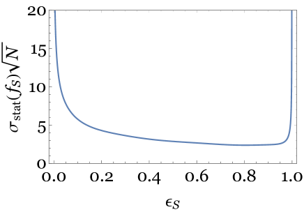
Figure 12: The statistical uncertainty in the inferred fraction of strange-quark jets times the square root of the total number of events for $f_{S}\simeq 0.95$ as a function of the strange-quark jet tagging efficiency for the CNN4 algorithm with $p_{T}=45$ GeV strange- and down-quark jets.

It is worthwhile to consider the performance of the binary tagging algorithms presented in this paper in a hypothetical background free measurement of the ratio of strange- to down-quark jets from a single isolated $W$-boson that decays hadronically to two resolved jets, where one of the jets is perfectly tagged as a charm-quark jet. While this is a highly idealized thought experiment that can not be achieved in reality in a high energy collider, it is none-the-less useful to illustrate the performance of strange- versus down-quark tagging algorithms. Neglecting the very small fraction of bottom-quark jets, the fraction of strange-quark jets in these decays is $f_{S}\simeq|V_{cs}|^{2}/(|V_{cs}|^{2}+|V_{cd}|^{2})\simeq 0.95$. The statistical uncertainty figure of merit (6.4) discussed in the previous sub-section, times the square root of the total number of events, all for this numerical value of the strange-quark jet fraction, is shown in Fig. 12 as a function of the strange-quark jet tagging efficiency for the CNN4 algorithm with $p_{T}=45$ GeV jets. In this hypothetical measurement, the best statistical precision in the inferred strange-quark jet fraction with this algorithm occurs for strange-quark jet tagging efficiencies roughly in the range $0.2-0.9$. Near the upper end of this range where the statistical precision is best, the reduced discriminating power of the tagging algorithm is overcome by increased statistics.

At the LHC hadronic decays of $W$-bosons are most easily isolated from backgrounds in production of a top-quark and anti-top quark with semi-leptonic decays of the resulting $W$-bosons, $t\bar{t}\to Wb\,Wb\to\ell\nu b\,jjb$. Half of the time one of the two non-bottom-quark resolved jets in this final state is a charm-quark jet (ignoring initial and final state radiation and jet overlaps). In this case, $t\bar{t}\to Wb\,Wb\to\ell\nu b\,jc\,b$, a fraction $f_{S}\simeq 0.95$ of the time the remaining resolved non-charm/bottom jet is a strange-quark jet, and a fraction $1-f_{S}\simeq 0.05$ of the time it is a down-quark jet (again ignoring initial and final state radiation and jet overlaps). These particular final states could be largely isolated from backgrounds and combinatoric confusion by requiring an isolated lepton, missing energy, at least four jets, two of which are bottom-quark tagged and one of which is charm-quark tagged along with kinematic constraints consistent with production and decay of a top-quark and anti-top quark and subsequent semi-leptonic cascade decays through $W$-bosons. Although to our knowledge charm-quark jet tagging has not been explicitly implemented in resolved hadronic top-quark reconstruction, it could be included. So the process $t\bar{t}\to Wb\,Wb\to\ell\nu b\,jc\,b$ along with the resolved top-quark reconstruction outlined above, could provide a final state with a jet that may be isolated kinematically and which a large fraction of the time is a strange-quark jet. This could provide an interesting arena in which to apply and validate strange-quark jet tagging at the LHC. Deployed in this way, the identification of strange-quark jets would have to be part of an all-jet tagging procedure that discriminated among all jet types. In this application this includes not only bottom- and charm-quark jets with displaced charged track vertices, but also other light-flavor and gluon jets from initial and final state radiation.

7 Discussion

Strange-quark tagging is the last largely unexplored problem in jet identification. In this paper we have demonstrated that jets initiated by strange- and down-quarks can on average be distinguished by utilizing observables available to the current generation of general purpose high energy collider detectors, such as CMS and ATLAS at the LHC. We presented strange- versus down-quark jet tagging algorithms based on single whole-jet variables, BDTs of a few whole-jet variables, and CNNs with jet images based on inputs from detector sub-systems. These algorithms rely primarily on the observation that strange-quark jets have a higher momentum weighted fraction of neutral kaons that do down-quark jets. This difference can be observed and exploited in a general purpose collider detector in two main ways. First, long-lived neutral kaons, $K_{L}$, that are more common in strange-quark jets, deposit energy primarily in the HCAL, while neutral pions that decay promptly to photon pairs, $\pi^{0}\to\gamma\gamma$, that are more common in down-quark jets deposit energy in the ECAL. So on average, strange-quark jets have a higher fraction of neutral hadronic energy, while down-quark jets have a higher fraction of neutral electromagnetic energy. Second, short-lived neutral kaons that decay-in-flight to charged pion pairs within the inner tracking region, $K_{S}\to\pi^{+}\pi^{-}$, can be identified. The reconstructed momentum fraction of these short-lived kaons is larger for strange-quark jets than for down-quark jets.

Strange-quark jet tagging, deployed as an element of an all-jet tagging procedure that discriminated among all jet types, could have applications to many new physics searches and measurements at high energy colliders. Forming event categories based on tagging algorithm output classifier variables can help to isolate sought out signals from backgrounds, always improves statistical uncertainties, and could even make new types of reconstruction and measurements possible. This could be especially beneficial in signatures with multiple jets. In particular, strange-quark jet tagging, in conjunction with bottom- and charm-quark tagging with displaced vertices, could help reduce combinatoric confusion in the reconstruction of resolved hadronic top-quark decays. For semi-leptonic top-quark anti-top quark signatures, hadronic top-quark reconstruction might be an interesting sub-process in which to attempt to demonstrate and validate strange-quark jet tagging at the LHC. Ultimately this might also make possible a direct measurement of the ratio of CKM matrix elements $|V_{cs}/V_{cd}|$ in hadronic $W$-boson decays within reconstructed hadronic top-quark decays. If possible, such a measurement would likely be limited by systematic rather than statistical uncertainties, but would be complementary to existing measurements of these individual CKM elements in meson decays that rely on hadronic form factors and lattice simulations [46, 47].

The focus of this work has been a demonstration of strange- versus down-quark jets using observables available in the current generation of general purpose high energy collider detectors. However, some special purpose detectors have detector elements that could provide additional observable handles to exploit in strange-quark jet tagging. A Cherenkov system, such as the one in the LHCb detector at the LHC, allows for charged particle discrimination, in particular between low to moderate momentum charged pions and charged kaons. While the momentum weighted sum of these two types of particles are very similar in strange- and down-quark jets, the individual momentum weighted fractions differ significantly, as can be seen clearly in Fig. 1. So charged particle identification with a Cherenkov system could provide further qualitative improvement over the performance of strange-quark jet tagging demonstrated here. Another possibility for achieving charged particle identification is with precise timing information for charged particles. This can be used to deduce a velocity, that in combination with the standard measurement of momentum from track curvature in the magnetic field, yields a measure of the charged particle mass. The timing capabilities planned for future upgrades to the CMS and ATLAS detectors should allow separation of charged pions and kaons up to a few GeV in momentum. Timing resolutions sometimes discussed for future detectors at future colliders could increase this separation out to much larger momenta. This additional handle on the charged particle content of jets could improve many measured features of jet physics, including strange-quark jet tagging.

References

- [1] R. Kogler et al., “Jet Substructure at the Large Hadron Collider: Experimental Review,” Rev. Mod. Phys. 91 no. 4, (2019) 045003, arXiv:1803.06991 [hep-ex].
- [2] P. T. Komiske, E. M. Metodiev, and M. D. Schwartz, “Deep learning in color: towards automated quark/gluon jet discrimination,” JHEP 01 (2017) 110, arXiv:1612.01551 [hep-ph].
- [3] T. Cheng, “Recursive Neural Networks in Quark/Gluon Tagging,” Comput. Softw. Big Sci. 2 no. 1, (2018) 3, arXiv:1711.02633 [hep-ph].
- [4] H. Luo, M.-x. Luo, K. Wang, T. Xu, and G. Zhu, “Quark jet versus gluon jet: deep neural networks with high-level features,” arXiv:1712.03634 [hep-ph].
- [5] P. T. Komiske, E. M. Metodiev, B. Nachman, and M. D. Schwartz, “Learning to classify from impure samples with high-dimensional data,” Phys. Rev. D98 no. 1, (2018) 011502, arXiv:1801.10158 [hep-ph].
- [6] K. Fraser and M. D. Schwartz, “Jet Charge and Machine Learning,” JHEP 10 (2018) 093, arXiv:1803.08066 [hep-ph].
- [7] E. M. Metodiev, B. Nachman, and J. Thaler, “Classification without labels: Learning from mixed samples in high energy physics,” JHEP 10 (2017) 174, arXiv:1708.02949 [hep-ph].
- [8] G. Kasieczka, N. Kiefer, T. Plehn, and J. M. Thompson, “Quark-Gluon Tagging: Machine Learning meets Reality,” arXiv:1812.09223 [hep-ph].
- [9] ATLAS Collaboration, G. Aad et al., “Performance of -Jet Identification in the ATLAS Experiment,” JINST 11 no. 04, (2016) P04008, arXiv:1512.01094 [hep-ex].
- [10] CMS Collaboration, A. M. Sirunyan et al., “Identification of heavy-flavour jets with the CMS detector in pp collisions at 13 TeV,” JINST 13 no. 05, (2018) P05011, arXiv:1712.07158 [physics.ins-det].
- [11] R. D. Field and R. P. Feynman, “A Parametrization of the Properties of Quark Jets,” Nucl. Phys. B136 (1978) 1. [,763(1977)].
- [12] D. Krohn, M. D. Schwartz, T. Lin, and W. J. Waalewijn, “Jet Charge at the LHC,” Phys. Rev. Lett. 110 no. 21, (2013) 212001, arXiv:1209.2421 [hep-ph].
- [13] W. J. Waalewijn, “Calculating the Charge of a Jet,” Phys. Rev. D86 (2012) 094030, arXiv:1209.3019 [hep-ph].
- [14] J. Thaler and K. Van Tilburg, “Identifying Boosted Objects with N-subjettiness,” JHEP 03 (2011) 015, arXiv:1011.2268 [hep-ph].
- [15] T. Plehn and M. Spannowsky, “Top Tagging,” J. Phys. G39 (2012) 083001, arXiv:1112.4441 [hep-ph].
- [16] L. G. Almeida, M. Backović, M. Cliche, S. J. Lee, and M. Perelstein, “Playing Tag with ANN: Boosted Top Identification with Pattern Recognition,” JHEP 07 (2015) 086, arXiv:1501.05968 [hep-ph].
- [17] J. Pearkes, W. Fedorko, A. Lister, and C. Gay, “Jet Constituents for Deep Neural Network Based Top Quark Tagging,” arXiv:1704.02124 [hep-ex].
- [18] G. Kasieczka, T. Plehn, M. Russell, and T. Schell, “Deep-learning Top Taggers or The End of QCD?,” JHEP 05 (2017) 006, arXiv:1701.08784 [hep-ph].
- [19] S. Macaluso and D. Shih, “Pulling Out All the Tops with Computer Vision and Deep Learning,” JHEP 10 (2018) 121, arXiv:1803.00107 [hep-ph].
- [20] G. Louppe, K. Cho, C. Becot, and K. Cranmer, “QCD-Aware Recursive Neural Networks for Jet Physics,” JHEP 01 (2019) 057, arXiv:1702.00748 [hep-ph].
- [21] S. Egan, W. Fedorko, A. Lister, J. Pearkes, and C. Gay, “Long Short-Term Memory (LSTM) networks with jet constituents for boosted top tagging at the LHC,” arXiv:1711.09059 [hep-ex].
- [22] A. Butter, G. Kasieczka, T. Plehn, and M. Russell, “Deep-learned Top Tagging with a Lorentz Layer,” SciPost Phys. 5 no. 3, (2018) 028, arXiv:1707.08966 [hep-ph].
- [23] M. Erdmann, E. Geiser, Y. Rath, and M. Rieger, “Lorentz Boost Networks: Autonomous Physics-Inspired Feature Engineering,” JINST 14 no. 06, (2019) P06006, arXiv:1812.09722 [hep-ex].
- [24] L. Moore, K. Nordström, S. Varma, and M. Fairbairn, “Reports of My Demise Are Greatly Exaggerated: -subjettiness Taggers Take On Jet Images,” SciPost Phys. 7 no. 3, (2019) 036, arXiv:1807.04769 [hep-ph].
- [25] B. M. Dillon, D. A. Faroughy, and J. F. Kamenik, “Uncovering latent jet substructure,” Phys. Rev. D100 no. 5, (2019) 056002, arXiv:1904.04200 [hep-ph].
- [26] P. T. Komiske, E. M. Metodiev, and J. Thaler, “Energy Flow Networks: Deep Sets for Particle Jets,” JHEP 01 (2019) 121, arXiv:1810.05165 [hep-ph].
- [27] H. Qu and L. Gouskos, “ParticleNet: Jet Tagging via Particle Clouds,” arXiv:1902.08570 [hep-ph].
- [28] E. A. Moreno, T. Q. Nguyen, J.-R. Vlimant, O. Cerri, H. B. Newman, A. Periwal, M. Spiropulu, J. M. Duarte, and M. Pierini, “Interaction networks for the identification of boosted decays,” arXiv:1909.12285 [hep-ex].
- [29] CMS Collaboration, “Machine learning-based identification of highly Lorentz-boosted hadronically decaying particles at the CMS experiment,” CMS-PAS-JME-18-002 (2019) .
- [30] ATLAS Collaboration, “Performance of top-quark and -boson tagging with ATLAS in Run 2 of the LHC,” Eur. Phys. J. C79 no. 5, (2019) 375, arXiv:1808.07858 [hep-ex].
- [31] A. Butter et al., “The Machine Learning Landscape of Top Taggers,” SciPost Phys. 7 (2019) 014, arXiv:1902.09914 [hep-ph].
- [32] J. Duarte-Campderros, G. Perez, M. Schlaffer, and A. Soffer, “Probing the strange Higgs coupling at colliders using light-jet flavor tagging,” arXiv:1811.09636 [hep-ph].
- [33] CMS Collaboration, V. Khachatryan et al., “CMS Tracking Performance Results from early LHC Operation,” Eur. Phys. J. C70 (2010) 1165–1192, arXiv:1007.1988 [physics.ins-det].
- [34] ATLAS Collaboration, G. Aad et al., “Kshort and production in interactions at and 7 TeV measured with the ATLAS detector at the LHC,” Phys. Rev. D85 (2012) 012001, arXiv:1111.1297 [hep-ex].
- [35] J. Alwall, M. Herquet, F. Maltoni, O. Mattelaer, and T. Stelzer, “MadGraph 5 : Going Beyond,” JHEP 06 (2011) 128, arXiv:1106.0522 [hep-ph].
- [36] T. Sjstrand, S. Ask, J. R. Christiansen, R. Corke, N. Desai, P. Ilten, S. Mrenna, S. Prestel, C. O. Rasmussen, and P. Z. Skands, “An Introduction to PYTHIA 8.2,” Comput. Phys. Commun. 191 (2015) 159–177, arXiv:1410.3012 [hep-ph].
- [37] M. Bahr et al., “Herwig++ Physics and Manual,” Eur. Phys. J. C58 (2008) 639–707, arXiv:0803.0883 [hep-ph].
- [38] J. Bellm et al., “Herwig 7.0/Herwig++ 3.0 release note,” Eur. Phys. J. C76 no. 4, (2016) 196, arXiv:1512.01178 [hep-ph].
- [39] DELPHES 3 Collaboration, J. de Favereau, C. Delaere, P. Demin, A. Giammanco, V. Lemaître, A. Mertens, and M. Selvaggi, “DELPHES 3, A modular framework for fast simulation of a generic collider experiment,” JHEP 02 (2014) 057, arXiv:1307.6346 [hep-ex].
- [40] M. Cacciari, G. P. Salam, and G. Soyez, “FastJet User Manual,” Eur. Phys. J. C72 (2012) 1896, arXiv:1111.6097 [hep-ph].
- [41] M. Cacciari, G. P. Salam, and G. Soyez, “The anti- jet clustering algorithm,” JHEP 04 (2008) 063, arXiv:0802.1189 [hep-ph].
- [42] S. Macaluso and D. Shih, “Pulling Out All the Tops with Computer Vision and Deep Learning,” arXiv:1803.00107 [hep-ph].
- [43] M. D. Zeiler, “ADADELTA: an adaptive learning rate method,” CoRR abs/1212.5701 (2012) , arXiv:1212.5701.
- [44] D. P. Kingma and J. Ba, “Adam: A method for stochastic optimization,” CoRR abs/1412.6980 (2014) , arXiv:1412.6980.
- [45] H. Qu and L. Gouskos, “ParticleNet: Jet Tagging via Particle Clouds,” arXiv:1902.08570 [hep-ph].
- [46] Particle Data Group Collaboration, M. Tanabashi et al., “Review of Particle Physics,” Phys. Rev. D98 no. 3, (2018) 030001.
- [47] S. Descotes-Genon and P. Koppenburg, “The CKM Parameters,” Ann. Rev. Nucl. Part. Sci. 67 (2017) 97–127, arXiv:1702.08834 [hep-ex].