Explained Variation under the Additive Hazards Model

Abstract

We study explained variation under the additive hazards regression model for right-censored data. We consider different approaches for developing such a measure, and focus on one that estimates the proportion of variation in the failure time explained by the covariates. We study the properties of the measure both analytically, and through extensive simulations. We apply the measure to a well-known survival data set as well as the linked Surveillance, Epidemiology and End Results (SEER)-Medicare database for prediction of mortality in early-stage prostate cancer patients using high dimensional claims codes.

1 Introduction

The additive hazards model [1, 2] has received increasing attention lately for the analysis of censored survival data. It is not just an alternative to the more widely used Cox model when the proportional hazards assumption is violated; it has also been argued to be more suitable for causal inferences in estimating treatment effects because the Cox model is not collapsible [3]. In contrast, the additive hazards model behaves mostly like a linear model including collapsibility, in the sense that one can integrate out an independent covariate from the model and still end up with an additive hazards model, with the same regression coefficients for all the other covariates. For this reason it has been used in the development of instrumental variable approaches for survival data including competing risks [4, 5, 6, jiang2018two, 7, 8]. The collapsibility as well as other behaviors similar to a linear model, has also enabled the additive hazards model to be used in mediation analysis of survival data [9, 10, 11, 12, 13]. In addition, doubly robust methods have been developed for estimating treatment effects and applied in practice under the additive hazards model including for optimal treatment regimes [14, 15, 16], while the noncollapsibility of the Cox model presents an obstacle in the development of doubly robust method when confounders are present [17].

Estimation and inference procedures have been well developed and implemented under the additive hazards model (eg. R package ‘timereg’), and diagnostic methods have also been proposed [18, 19, 20]. However, another important aspect as the model becomes more widely used, is explained variation or measures of predictability, often referred to as $R^{2}$. O’Quigley and Xu [21] provide detailed illustrations of how such measures are used to evaluate the clinical importance of prognostic factors. Müller et al. [22] and Hielscher et al. [23] explored the use of $R^{2}$ measures in genetic studies to quantify the impact of genetic variants or high dimensional gene expression on survival phenotypes, while Preseley et al. [24] applied them to surrogate evaluation. Very recently applications of measure of dependence to ultrahigh dimensional variable screening were explored in Kong et al. [25]. In the context where the estimation of treatment effect is of primary concern, following the fit of the additive hazards models it is also natural to provide estimates of predicted survival given the covariates [8]. However, measures of explained variation have not been examined under the additive hazards model to our best knowledge.

Explained variation has been well studied in the literature under the Cox regression model for right-censored data. Kent and O’Quigley [26] first defined a measure of dependence for censored survival data, making use of the Kullback-Leibler information gain. It is based on the conditional distribution of the time to event random variable $T$ given the covariates $Z$. A later work by Xu and O’Quigley [27] considered instead the conditional distribution of $Z$ given $T$, using also the information gain. This latter measure can be readily extended to time-dependent covariates. A simple approximation to this second measure was described in O’Quigley et al. [28], which can be easily computed using the partial likelihood ratio test statistic following the fit of the Cox model. Preseley et al. [24] advocated for these information gain based measures.

Another approach to defining explained variation makes use of the residuals. This originated from the $R^{2}$ under the linear regression model, which can be written as one minus the ratio of the residual sum of squares over the total sum of squares. It is also well-known that these two sums of squares estimate the residual variance and the total variance, respectively. O’Quigley and Flandre [29] proposed to use the Schoenfeld residuals under the Cox model, in a similar way to the $R^{2}$ under linear regression. It has been shown that when the Cox model appears to be a reasonably fit to the data, this measure and the one above based on information gain, tend to give comparable quantifications of explained variation [21].

Other approaches have also been considered in the literature for right-censored data. Schemper and Kaider [30] proposed to compute the correlation coefficients between the failure rankings and the covariates, using multiple imputation to handle the censored data. We note that inference under the Cox model is only based on the ranks of the failure times, hence nonparametric correlation coefficients like Kendall’s tau or Spearman correlation might be considered. However, as it is known and we also elaborate below, inference under the additive hazards model is not rank based.

Finally and not restricted to the survival context, previous experiences in describing explained variation outside the classic linear model have also considered the direct decomposition of the total variance in the outcome, and quantifying the proportion that is explained by the covariates. Depending on the model, this can sometimes be a straightforward approach, such as under the linear mixed effects model [31, 32], or under the accelerated failure time (AFT) models [33].

In this work we consider the semiparametric additive hazards model. We aim to quantify the explained variation under this model. It turns out that the last approach described above, i.e. the direct decomposition of the total variation into components of explained and unexplained (or residual) variation, is easily computable as well as interpretable under the additive hazards model. In the following we will first focus on its development, investigate its properties, and illustration how it might be used in practice to quantify the predictive power of a set of prognostic variables, and also for use in variable selection procedures. We will defer discussion to the end of the paper why some of the other approaches described above do not work under the additive hazards model.

The rest of the paper is organized as follows. After a review of the semiparametric additive hazards model and its inference in the next section, we describe explained variation and its estimator in section 3. In section 4, we study the properties of the measure, both the population and the sample-based versions. Section 5 further explores the behavior of the measures using simulation, under different censoring scenarios, different covariate distributions, different baseline hazard functions, and beyond. We apply the measure to real data sets in Section 6, and we conclude with discussion in the last section.

2 Semiparametric Additive Hazards Model

Let $T$ be the failure time random variable of interest, $Z$ be a vector of covariates, and $C$ be the censoring time random variable. Let $X=\min{\left(T,C\right)}$ and $\delta=I{(T\leq C)}$ where $I(\cdot)$ is the indicator function. We observe a random sample $(X_{i},Z_{i},\delta_{i})$, $i=1,\ldots,n$. The semiparametric additive hazards model [34] assumes that the conditional hazard function

$$\lambda(t|Z)=\lambda_{0}(t)+\beta^{\top}Z,$$ (1)

where $\lambda_{0}(t)$ is the baseline hazard and $\beta$ is a vector of regression effects. We will also use the counting process notation: $N(t)=I{\left\{X\leq t,\delta=1\right\}}$ and $Y(t)=I{\left\{X\geq t\right\}}$ are the counting process of events and the at-risk process, respectively.

Under model (1), an estimator for $\beta$ was proposed by Lin and Ying [34]:

$$\hat{\beta}=\left[\sum_{i=1}^{n}\int_{0}^{\infty}Y_{i}(t)\left\{Z_{i}-\bar{Z}(t)\right\}^{\otimes 2}dt\right]^{-1}\left[\sum_{i=1}^{n}\int_{0}^{\infty}\left\{Z_{i}-\bar{Z}(t)\right\}dN_{i}(t)\right],$$ (2)

where $\bar{Z}(t)=\sum_{i=1}^{n}{Y_{i}(t)Z_{i}}/{\sum_{i=1}^{n}Y_{i}(t)}$. We note that unlike under the Cox model, the above estimator of $\beta$ is not rank based in that it depends on the values of $X_{i}$’s beyond their ranks in the data set. It can be shown that, if $g(\cdot)$ is a strictly increasing function, then $g(T)$ in general no longer follows a semiparametric additive hazards model. In the special case where $g$ is multiplication by a constant $c>0$, then $\tilde{T}=cT$ still follows a semiparametric additive hazards model, but the regression coefficient is rescaled by c: $\tilde{\beta}=\beta/c$.

The cumulative baseline hazard function $\Lambda_{0}(t)=\int_{0}^{t}\lambda_{0}(u)du$ is estimated by

$$\tilde{\Lambda}_{0}(t)=\int_{0}^{t}\frac{\sum_{i=1}^{n}\left(dN_{i}(u)-Y_{i}(u)\hat{\beta}(u)^{\top}Z_{i}du\right)}{\sum_{j=1}^{n}Y_{j}(u)}.$$ (3)

In the following we write out the integral in (3), which is not a step function. Denote the $K$ ordered distinct observed failure times $t_{1}<...<t_{K}$. We have for $k=1,...,K$:

$$\tilde{\Lambda}_{0}(t_{k})=\sum_{l=1}^{k}\frac{\delta_{l}d_{l}}{r_{l}}-\sum_{l=1}^{k}\hat{\beta}^{\top}\bar{Z}\left(t_{l}\right)\left(t_{l}-t_{l-1}\right),$$ (4)

where $d_{l}$ and $r_{l}$ are the number of events and number at risk at time $t_{l}$, respectively. In addition, for any $t_{k}\leq t<t_{k+1}$,

$$\tilde{\Lambda}_{0}(t)=\sum_{l=1}^{k}\frac{\delta_{l}d_{l}}{r_{l}}-\sum_{l=1}^{k}\hat{\beta}^{\top}\bar{Z}\left(t_{l}\right)\left(t_{l}-t_{l-1}\right)-\hat{\beta}^{\top}\bar{Z}\left(t_{k+1}\right)\left(t-t_{k}\right).$$ (5)

The resulting estimated survival function $\tilde{S}(t|z)=\exp{(-\tilde{\Lambda}_{0}(t)-\hat{\beta}\top zt)}$ is not guaranteed to be non-increasing; therefore we make use of the following adjusted version [34]: $\hat{S}(t|z)=\min_{s\leq t}\left\{\tilde{S}(s|z)\right\}$. The adjusted version $\hat{S}$ is asymptotically equivalent to $\tilde{S}$, and the process $\sqrt{n}(\hat{S}(\cdot|z)-{S}(\cdot|z))$ converges wealy to a zero-mean Gaussian process [34]. We note that taking minimum over $s\leq t$ leads to no closed-form expression and the quantity needs to be computed numerically. However, it is imperative that we work with a proper distribution or equivalently, survival, function, in order to estimate the moments below.

3 Explained Variation

The explained variation, as described in the survival context by O’Quigley and Xu [21], can be defined as

$$\Omega^{2}=1-\frac{E\left\{\mbox{Var}(T\mid Z)\right\}}{\mbox{Var}(T)}=\frac{\mbox{Var}\left\{E(T\mid Z)\right\}}{\mbox{Var}(T)}.$$ (6)

This is consistent with the regression setting of model (1) for the conditional distribution of $T$ given $Z$, as the proportion of variation of $T$ explained by $Z$ out of the total variation of $T$. As pointed out in O’Quigley [35] page 33, by virtue of the Chebyshev-Bienayme inequality, the variance can be seen as a measure of predictability, and therefore the explained variation may also have an interpretation as predictability.

In practice for survival studies, there is often a finite upper bound of time $\tau$ due to administrative censoring, so that all the observable data are conditional upon $T<\tau$. We then define

$$\Omega^{2}_{\tau}=1-\frac{{E}\left\{\mbox{Var}(T\mid Z,T<\tau)\right\}}{\mbox{Var}(T\mid T<\tau)}=\frac{\mbox{Var}\left\{{E}(T\mid Z,T<\tau)\right\}}{\mbox{Var}(T\mid T<\tau)}.$$ (7)

Obviously when there is no censoring, $\Omega^{2}=\Omega^{2}_{\infty}$; and in the following for uniformity of notation, we allow $\tau\leq\infty$.

We can estimate directly the quantities in (7) under model (1). To estimate $E\left\{\mbox{Var}(T\mid Z,T<\tau)\right\}$ or
$\mbox{Var}\left\{E(T\mid Z,T<\tau)\right\}$, we first integrate with respect to an estimated distribution of $T$ given $Z$ and $T<\tau$:

$$\hat{S}(t\mid Z,T<\tau)=\frac{\hat{S}(t\mid Z)-\hat{S}(t_{K}\mid Z)}{1-\hat{S}(t_{K}\mid Z)}\mathbb{1}\left\{t\leq t_{K}\right\}$$ (8)

We then integrate with respect to $\mathbb{P}_{n}$, the empirical distribution of $Z$. Denote the resulting estimates ${E}_{n}\left\{\widehat{\mbox{Var}}\left(T\mid Z,T<\tau\right)\right\}$ and $\mbox{Var}_{n}\left\{\hat{{E}}(T\mid Z,T<\tau)\right\}$, respectively. For example,

$${E}_{n}\left\{\widehat{\mbox{Var}}\left(T\mid Z,T<\tau\right)\right\}=\frac{1}{n}\sum_{i=1}^{n}\left[{\hat{E}\left(T^{2}\mid Z_{i},T<\tau\right)}-\left\{{\hat{E}\left(T\mid Z_{i},T<\tau\right)}\right\}^{2}\right],$$ (9)

where the expressions for the quantities in the right-hand side above are given later in the section.

To estimate $\mbox{Var}(T\mid T\leq\tau)$, we can use

$$\widehat{\mbox{Var}}\left(T\mid T<\tau\right)={\hat{E}\left(T^{2}\mid T<\tau\right)}-\left\{{\hat{E}\left(T\mid T<\tau\right)}\right\}^{2}.$$ (10)

In order to estimate the marginal survival function, we may use the nonparametric Kaplan-Meier (KM) estimator. Alternatively, we may use:

$$\hat{S}(t\mid T<\tau)=\frac{1}{n}\sum_{i=1}^{n}\hat{S}(t\mid Z_{i},T<\tau).$$ (11)

It can be shown that, if (11) is used in estimating the expectations in (10), then we have the following decomposition:

$$\widehat{\mbox{Var}}(T\mid T<\tau)={{E}_{n}\left\{\widehat{\mbox{Var}}\left(T\mid Z,T<\tau\right)\right\}}+{\mbox{Var}_{n}\left\{\hat{E}(T\mid Z,T<\tau)\right\}}.$$ (12)

Combining all of the above, we obtain $R^{2}_{\tau}$ as a consistent estimator of $\Omega^{2}_{\tau}$ under model (1):

$$R^{2}_{\tau}=1-\frac{{{E}_{n}\left\{\widehat{\mbox{Var}}\left(T\mid Z,T<\tau\right)\right\}}}{\widehat{\mbox{Var}}\left(T\mid T<\tau\right)}=\frac{{\mbox{Var}_{n}\left\{\hat{E}\left(T\mid Z,T<\tau\right)\right\}}}{\widehat{\mbox{Var}}\left(T\mid T<\tau\right)}.$$ (13)

We also denote $R^{2}=R^{2}_{\infty}$ when $\tau=\infty$.

Finally, to compute the quantities in (13), we have:

$${\hat{E}\left(T\mid z,T<\tau\right)} = \int_{0}^{\tau}\hat{S}\left(t\mid z,T<\tau\right)dt$$ (14)

$$= \frac{1}{1-\hat{S}\left(t_{K}\mid z\right)}\int_{0}^{t_{K}}\hat{S}\left(t\mid z\right)dt-\frac{1}{1-\hat{S}\left(t_{K}\mid z\right)}\hat{S}\left(t_{K}\mid z\right)t_{K},$$

and

$${\hat{E}\left(T^{2}\mid z,T<\tau\right)} = 2\int_{0}^{\tau}t\cdot\hat{S}(t\mid z,T<\tau)dt$$ (15)

$$= \frac{2}{1-\hat{S}\left(t_{K}\mid z\right)}\int_{0}^{t_{K}}t\hat{S}\left(t\mid z\right)dt-\frac{1}{1-\hat{S}\left(t_{K}\mid z\right)}\hat{S}\left(t_{K}\mid z\right)t_{K}^{2}.$$

Since there is no closed-form expression for $\hat{S}(t\mid Z)$, the integrals in the above are computed using the trapezoidal rule. We partition the interval $[0,\tau]$ first using $t_{1},\ldots,t_{K}$; additional points are added to create a grid no wider than 0.01 between two adjacent points. We then use an iterative halving process, i.e. adding the midpoints between any two adjacent points to the grid, until the change in the resulting $R^{2}_{\tau}$ is less than 0.01 in absolute value.

The quantities in $\widehat{\mbox{Var}}(T\mid T<\tau)$ can be computed in a similar fashion using (11).

4 Properties of $\Omega^{2}$ and $R^{2}$

The desirable properties of a measure of explained variation are best understood under a linear regression model, including: 1) it lies between zero and one; 2) it takes the value zero when there is no regression effect; 3) it increases with the strength of the regression effect; 4) it tends to one as the regression effect tends to infinity; 5) it is invariant under certain transformations of the dependent and independent variables, depending on the model. For the last property, the transformation is linear under the linear regression model, and is rank-preserving for the failure time under the semiparametric Cox regression model [21].

In the following we investigate if the above properties hold for the measures defined in the last section.

• The facts that $0\leq\Omega^{2}_{\tau}\leq 1$ and $0\leq R^{2}_{\tau}\leq 1$ follow immediately from their definitions (7) and (13), assuming that the latter is estimated using (11).

• When $\beta=0$, $\Omega^{2}_{\tau}=0$ because independence between $T$ and $Z$ implies that $\mbox{Var}\{E(T\mid T<\tau,Z)\}=\mbox{Var}\{E(T\mid T<\tau)\}$. Also $R^{2}_{\tau}=0$ if it happens that the estimated coefficient $\hat{\beta}=0$. Otherwise, the sample based measure $R^{2}_{\tau}>0$, but is expected to be small since it is a consistent estimate of $\Omega^{2}_{\tau}=0$.

• It is analytically difficulty to prove that $\Omega^{2}_{\tau}$ increases with $|\beta|$ in general. However, for simpler settings such as a binary $Z$ and $\tau=\infty$, we can prove it analytically and this is given in the Appendix. For more general settings, we illustrate this via simulation.

• It has been known that the quantity $\Omega^{2}$ defined in (6) can be bounded strictly less than one [21]. For a binary $Z$, if we assume that $T\mid Z=0$ has finite second moment, then we can show by the dominated convergence theorem that:

  $$\lim_{\beta\rightarrow\infty}\Omega^{2}_{\infty}=1-\frac{\frac{1}{2}\left[2\int_{0}^{\infty}t\exp{\left\{-\Lambda_{0}(t)\right\}}dt-\left[\int_{0}^{\infty}\exp{\left\{-\Lambda_{0}(t)\right\}}dt\right]^{2}\right]}{\int_{0}^{\infty}t\exp{\left\{-\Lambda_{0}(t)\right\}}dt-\frac{1}{4}\left[\int_{0}^{\infty}\exp{\left\{-\Lambda_{0}(t)\right\}}dt\right]^{2}}.$$ (16)

  For example, when $\lambda_{0}(t)=1$, $\lim_{\beta\rightarrow\infty}\Omega^{2}_{\infty}=0.333$; and this is the exponential case discussed in O’Quigley and Xu [21]. When $\lambda_{0}(t)=t$, $\lim_{\beta\rightarrow\infty}\Omega^{2}_{\infty}=0.647$; and when $\lambda_{0}(t)=1/(2\sqrt{t})$, $\lim_{\beta\rightarrow\infty}\Omega^{2}_{\infty}=0.091$. Similar calculation can be done for covariates with continuous distribution:

  $$\lim_{\beta\rightarrow\infty}\Omega^{2}_{\infty}=1-\lim_{\beta\rightarrow\infty}\frac{\int_{\mathcal{Z}}\left[\int_{0}^{\infty}2t\exp{\left\{-\Lambda_{0}(t)-\beta^{\top}Zt\right\}}dt-\left[\int_{0}^{\infty}\exp{\left\{-\Lambda_{0}(t)-\beta^{\top}Zt\right\}}dt\right]^{2}\right]g(z)dz}{\int_{\mathcal{Z}}\int_{0}^{\infty}2t\exp{\left\{-\Lambda_{0}(t)-\beta^{\top}Zt\right\}}dtg(z)dz-\left[\int_{\mathcal{Z}}\int_{0}^{\infty}\exp{\left\{-\Lambda_{0}(t)-\beta^{\top}Zt\right\}}dtg(z)dz\right]^{2}},$$ (17)

  where $g(Z)$ is the density of the covariates and $\mathcal{Z}$ is their sample space. This limit may not be equal to one and it depends on the form of $\lambda_{0}(t)$ and the distribution of $Z$; for example, when $Z\sim U\left[0,\sqrt{3}\right]$ and $\lambda_{0}(t)=1$, $\lim_{\beta\rightarrow\infty}\Omega^{2}_{\infty}=0.500$.

• By their definitions and simple algebra, it can be shown that $\Omega^{2}_{\tau}$ and $R^{2}_{\tau}$ are invariant under linear transformations of $Z$ and when $T$ is rescaled by a positive constant.

In summary, we have the following properties:

• $0\leq\Omega^{2}_{\tau}\leq 1$, and $0\leq R^{2}_{\tau}\leq 1$;

• $\Omega^{2}_{\tau}=0$ when $\beta=0$, and $R^{2}_{\tau}=0$ if $\hat{\beta}=0$;

• $\Omega^{2}_{\tau}$ increases with $|\beta|$;

• $\Omega^{2}_{\tau}$ and $R^{2}_{\tau}$ are invariant under any linear transformation of $Z$ and rescaling of $T$.

5 Simulations

In the following we further study the properties of the measures through simulations. In addition to the properties mentioned above, we also investigate: 1) the effect of baseline hazard on explained variation; 2) explained variation under nested models. As we have more experience with explained variation under the Cox proportional hazards regression model, we also investigate 3) how the measure compares with a similar one under the Cox model, when both models are valid; and 4) explained variation of $Z$ give $T$, which has been advocated for use under the Cox model.

All simulations below were carried out with sample size 1000, and 100 simulation runs each. All the results are reported as mean with standard deviation (SD) over the simulation runs in $(\cdot)$. As the simulation has been extensive, we have chosen to display the representative scenarios that carry meaningful messages, as opposed to every combination of all possible parameters and settings.

5.1 Basic properties

As $|\beta|$ increases

We first simulated with $\lambda_{0}(t)=1$ and different values $\beta=$1, 3, 15 and 50, $Z$ from Uniform $[0,\sqrt{3}]$ as well as binary 0,1 with equal probabilities. Note that these two covariate distributions have the same variance 0.25, rendering the measures comparable for a given $\beta$ value. The censoring distribution was uniform $[0,\tau]$. We computed the $\Omega^{2}_{\tau}$ values as follows. When there was no censoring we computed it analytically by definition using the fact that $T\sim$ Exponential ($1+\beta Z$). When there was censoring, we took a single large sample size of 100,000, and used the $R^{2}_{\tau}$ value computed with the true $\beta$ and the true $\lambda_{0}$ to approximate $\Omega^{2}_{\tau}$.

From Figure 1 and Table Explained Variation under the Additive Hazards Model we see that $R^{2}_{\tau}$ and $\Omega^{2}_{\tau}$ values are close in all cases, both increasing with $|\beta|$ as expected. The effect of $\tau$ reflects different follow-up periods, which also leads to different amounts of censoring. It is seen that the patterns of change with $\tau$ is different depending on the distribution of $Z$. It is more pronounced with binary $Z$ especially for that larger $\beta$ values, likely because the censor percentages are much higher in that case.

Effect of $\lambda_{0}(\cdot)$

We consider here a binary $Z$ taking values 0,1 with equal probabilities. We consider $\lambda_{0}(t)=1$, $t$ and $1/(2\sqrt{t})$. In Figure 2 we plot the density of $T$ for each group, to show how the two groups differ in each scenario. The mean of $R^{2}_{\infty}$ over the 100 simulations are printed on each configuration. From Figure 2 we see that the $R^{2}_{\infty}$ values tend to be larger when the two groups indexed by $Z=0$, 1 have different concentrations of failure times, i.e. different shapes of the density functions, such as in the case of $\lambda_{0}(t)=t$. On the contrary, with $\lambda_{0}(t)=1/(2\sqrt{t})$ the two density functions have very similar shapes, resulting much smaller $R^{2}_{\infty}$ values. As noted earlier, the upper bound of $\Omega^{2}$ for the three cases are 0.091, 0.333 and 0.647, respectively.

Nested models

Next we consider a limited set of simulations with data generated under $\lambda(t|Z)=\lambda_{0}(t)+Z_{1}+3Z_{2}+Z_{3}$, where the covariates $Z_{1},Z_{2}$ and $Z_{3}$ were independently drawn from Uniform $[0,\sqrt{3}]$ and the baseline hazard was in turn equal to $1,t$ and $1/(2\sqrt{t})$. We also consider an additional pure noise covariate $Z_{4}\sim$ Uniform $[0,\sqrt{3}]$, not used in the data generating mechanism. We consider the following models listed in Table 2: three univariate models with each of $Z_{1},Z_{2}$ and $Z_{3}$, respectively; a model with only $Z_{1}$ and $Z_{3}$; a model with all the three $Z_{1},Z_{2},Z_{3}$; and a model with the three covariates plus the pure noise $Z_{4}$. We see from Table 2 that $R^{2}_{\infty}$ increases with the complexity of the models: $R^{2}_{\infty}$ with both $Z_{1}$ and $Z_{3}$ is larger than with $Z_{1}$ or $Z_{3}$ alone; meanwhile, since $Z_{2}$ has a strong effect as reflected in its regression coefficient, $R^{2}_{\infty}$ with $Z_{2}$ alone is larger than with both $Z_{1}$ and $Z_{3}$. The measure is substantially larger with all three covariates $Z_{1},Z_{2}$ and $Z_{3}$ than under any of the previous models. With the noise variable $Z_{4}$ added to the model, $R^{2}_{\infty}$ increases very slightly from 0.122 to 0.124, for example. This also informs us how to use the $R^{2}$ type measures for model selection: if the addition of a variable only increases the $R^{2}$ very slightly, it is perhaps not worth the cost of an extra degree of freedom. This is consistent with the concept of adjusted $R^{2}$, which explicit adjusts for the number of degrees of freedom. We further discuss this in the applications later.

5.2 Comparison with the measure under the Cox Model

As discussed earlier the semiparametric additive hazards model behaves somewhat differently from the semiparametric Cox model. Here we compare $R^{2}_{\tau}$ as defined in (13) under the two models when both models are valid. We consider a binary $Z$ and constant baseline hazard; this is a case where both the semiparametric additive hazards model (1) and the classic Cox model hold.

Under the Cox model $S(t\mid Z)=\{S_{0}(t)\}^{\exp(\beta Z)}$, where the regression parameter is typically estimated using the partial likelihood, and the baseline survival function via the Breslow’s estimate of the cumulative baseline hazard. We can then similarly estimate the explained variation as defined in (6) or (7), using a similar approach as described in Section 3. We denote this as $R^{2}_{cox}$. Both $R^{2}_{cox}$ and $R^{2}_{\tau}$ thus defined should be consistent for the same $\Omega^{2}_{\tau}$. In Table 3 we again simulated with $\lambda(t|Z)=1+\beta Z$ for a binary $Z$, $\beta=1,3,15$ and 50, with no censoring or $30\%$ censoring . As expected, the values of $R^{2}_{cox}$ and $R^{2}_{\tau}$ are indeed very close to each other.

5.3 Explained variation of $Z$ given $T$

O’Quigley and Xu [21] advocated for considering the explained variation of $Z$ given $T$ under the Cox regression model. One main advantage of this approach is that the resulting measure tend not to be bounded strictly less than one. In addition, considering $Z$ given $T$ is also consistent with the sequential conditioning and counting process notation often used in survival analysis. Following O’Quigley and Flandre [29] and O’Quigley and Xu [21], we consider in particular the covariate residual (also called Schoenfeld residual under the Cox model) based approach.

In order to obtain the residuals of $Z$, we need to estimate the conditional distribution of $Z$ given $T$. A theorem from Xu and O’Quigley [27, 36] can be readily adapted to provide a consistent estimate of this conditional distribution under model (1):

Theorem 1

Under model (1) and independent censoring, assuming that $\lambda_{0}(t)$ is known (or otherwise consistently estimated), the conditional distribution of Z given T is consistently estimated by

$$\hat{P}(Z\leq z\mid T=t)=\frac{\sum_{Z_{j}\leq z}Y_{j}(t)\left(\lambda_{0}(t)+\hat{\beta}^{T}Z_{j}\right)}{\sum_{l=1}^{n}Y_{l}(t)\left(\lambda_{0}(t)+\hat{\beta}^{T}Z_{l}\right)}.$$ (18)

The proof of the above theorem is similar to that of Theorem 1 in Xu and O’Quigley [27, 36] but applied to model (1).

In practice $\lambda_{0}(t)$ is unknown, and also not readily estimated by the typical software that fit the additive hazards model. Our investigation here is of exploratory nature, aimed to understand the behaviors of the explained variation of $T$ give $Z$ versus $Z$ given $T$. In simulations below we use the true $\lambda_{0}(t)$. Denote

$$\hat{E}_{\beta}\left(Z\mid t\right)=\frac{\sum_{j=1}^{n}Z_{j}Y_{j}(t)\left(\lambda_{0}(t)+\beta Z_{j}\right)}{\sum_{l=1}^{n}Y_{l}(t)\left(\lambda_{0}(t)+\beta Z_{l}\right)}.$$ (19)

The residuals under the fitted model and under the ‘null’ model where $\beta=0$ are, respectively:

$$r_{i}(\hat{\beta})=Z_{i}-\hat{E}_{\hat{\beta}}\left(Z\mid X_{i}\right),\,\,\,r_{i}(0)=Z_{i}-\hat{E}_{0}\left(Z\mid X_{i}\right),$$ (20)

where ${E}_{0}\left(Z\mid X_{i}\right)$ is simply the empirical average of $Z$ in the risk set at time $X_{i}$. Therefore for a scalar $Z$ we may define

$$R^{2}_{Z\mid T}=1-\frac{\sum_{i=1}^{n}r^{2}_{i}(\hat{\beta})}{\sum_{i=1}^{n}r^{2}_{i}(0)}.$$

The extension to multivariate $Z$ was described in O’Quigley and Xu [21] and can be easily adopted here.

We simulated under $\lambda(t)=1+\beta Z$, with a binary $Z$ and equal probabilities of 0, 1. In Table 4 we see that unlike $R^{2}_{\tau}$, the values of $R^{2}_{Z\mid T}$ approach one with increasing $|\beta|$. We further discuss the unknown $\lambda_{0}(t)$ in the last section.

6 Applications

6.1 Leukimia: FREIREICH DATA

We first apply the measure of explained variation to the Freireich et al. [37] data, which consist of the remission times of 42 Leukimia patients in a randomized clinical trial treated with the drug 6-mercaptopurine (6-MP) versus placebo. The data set has been well-known in the survival analysis literature, and was in the first table of Cox and Oakes [38]. As a diagnostic plot in Figure 3 we show the difference of the cumulative hazard functions between the two treatment groups; under the semiparametric additive hazards model (1) this difference should be linear in time. From the figure we see that except for random noise due to limited sample size the difference shows a very nice linear trend, indicating that the semiparametric model (1) fits the data reasonably well. We note that in the R package ‘timereg’ that we used to fit the semiparametric additive hazards model, no diagnostic tools appear to be provided for checking this model.

We calculated $R^{2}=0.201$, indicating, as is known, good separation between the two groups’ survival times. Typically if a single predictor, in particular a binary one, turns out to have an $R^{2}$ of around 20% say, it is considered to be a strong predictor. Previously the explained variation of $Z$ given $T$ under the Cox regression model had been calculated to be around 0.40 (ranging from 0.38 to 0.42 depending on the measure used) [21]. The Freireich data appears to be a data set that fits both the proportional hazards model and the additive hazards model reasonably well. Based on the simulation results, when the data fits both models, the explained variation of $T$ given $Z$ would be very close under the two models. The discrepancy between the $R^{2}$ values seen above are most likely attributable to the difference between the explained variation of $Z$ given $T$ and that of $T$ given $Z$, as also illustrated in the simulations. In this case they otherwise reflect somewhat comparable strengths of association in our opinion.

6.2 Prostate cancer: SEER-MEDICARE DATA

We study the time to death of 29,657 prostate cancer patients with localized non-metastatic disease identified from the linked Surveillance, Epidemiology, and End Results (SEER) - Medicare database, diagnosed between 2004 and 2009. Following Hou et al. [39] we consider the clinical and the demographical variables, plus the binary insurance claims codes from Medicare. The latter captures medical diagnoses and procedures through Healthcare Common Procedure Coding System (HCPCS) codes, international classification of diseases (ICD)-9 diagnosis and procedure codes, etc. Each insurance claims code variable takes value one if that claim appeared within one year before diagnosis, and zero otherwise. Out of the 29,657 patients 3,543 died by the end of the follow-up which was December 2013 when the data were exported from the linked database.

The high dimensional data analysis of Hou et al. [39] selected 143 variables to predict non-cancer mortality, and 9 variables to predict cancer mortality, in the context of these two competing risks. The same sets of variables were used in Riviere et al. [40] and a complete list can be found in Table 1 and 2 of their supplemental material. For our analysis of explained variation, we combined these two sets of predictor for overall survival, which resulted in 146 variables: PSA, Gleason Score, age, race (black versus other), marital status (married versus other) and registry (California versus other), plus the claims codes. A table with the distributions of these variables can be found in the Supplemental Materials.

In Figure 5 we plot the difference of the cumulative hazard functions between groups as we did for the Freireich data above, to check the additive hazards model assumption. These are illustrated for six binary variables, the three demographical variables plus three claims codes that are not too sparse to plot. The plots indicate that the model seems to fit the data reasonably well.

We consider three models here. We first fit the data to the semiparametric additive hazards model with only the cancer-related clinical variables PSA and Gleason Score. We then add the four demographical variables. Finally we added the set of claim codes. The model fits are provided in the tables of the Supplement Materials. Table 5 summarizes the $R^{2}$ values obtained under these three models. In the first column of the table we see that the cancer-related clinical variables alone do not explain much (under 1%) variation in overall survival. This can at least be partially understood since only 734 out of the 3,543 total deaths in this data set were due to cancer. Demographical variables, on the other hand, do explain a substantial amount of variation in overall survival. This amount of explained variation is further increased, by a non-trivial amount, after adding in the claims codes previously identified from the high-dimensional SEER-Medicare database.

When high dimensional claims codes are used in the data analysis, there is often the concern of model over-fitting. In our case, with 3,543 death events and 146 total regressors, this may not be an issue. Nonetheless, we proceed to divide the data set randomly into two parts, a training set with 14,828 observations containing 1,803 deaths, and a test set with 14,829 observations containing 1740 deaths. We fit the additive hazards model to the training data set and obtain the estimates $\hat{\beta}$ and $\hat{\Lambda}_{0}(t)$. We use them to compute $\hat{S}(t|Z)$ on the test data set, and obtain an out-of-sample $R^{2}_{out}$. Such out-of-sample $R^{2}$ measures are often used in machine learning applications (eg. deep learning) in order to reduce the risk of overfitting. We report the $R^{2}_{out}$ in Table 5. It is seen that, for this data, the $R^{2}_{out}$ values are in fact slightly higher than the $R^{2}$ computed on the full data set, or the $R^{2}_{train}$ computed on the training data set. Were there over-fitting, the $R^{2}_{out}$ values would have been substantially lower. The discrepancy among the three quantities currently seen is mostly due to variability in the estimation of the conditional survival function and consequently of the total and explained variances. For comparison purposes, we also provide in the Supplemental Materials the three model fits to the training data set. We can compare the estimated coefficients with those using the full data set, and observe that the estimates for the statistically signficant ones are stable across the training versus the full data set.

At the suggestion of a reviewer, we compute the adjusted $R^{2}$, $R^{2}_{adj}=1-(1-R^{2})(n-1)/(n-p-1)$, for the three models. Here $n$ is the sample size, and $p$ is the number of the covariates included in the model. The $R^{2}_{adj}$ is computed on the full data set. By definition $R^{2}_{adj}<R^{2}$, although no difference can be seen at three digits after the decimal point between the two measures for the first two models since $p$ is so small compared to $n$. For the third model that includes 146 variables, the difference of 0.3% between the two does not appear to signify any over-fitting.

Finally we note that the explained variation of $Z$ given $T$ under the Cox model, denoted $\rho^{2}$, was calculated in Riviere et al. [40] for this data. They computed $\rho^{2}=0.71$ for cancer mortality and $\rho^{2}=0.60$ for non-cancer mortality under competing risks setting. As discussed before, the numerical values of explained variation of $T$ given $Z$ are not directly comparable to those of $Z$ given $T$. Considering that the former has an upper bound less than one, it is perhaps also within reasons to conclude that our analysis under the additive hazards model agrees with that of Riviere et al. [40] about the contribution of the claims codes in explaining overall mortality for this prostate cancer patient population. This conclusion echoes the initial goal of the funded project that lead to the previous publications [39, 40] to demonstrate that the high-dimensional insurance claims codes contain useful information about mortality in this patient population.

7 Discussion

In this paper we have studied explained variation under the semiparametric additive hazards model for right-censored survival data. The explained variation is shown to lie between zero and one, and to increase with the magnitude of the regression effect. It has been known, and is shown again here, that the explained variation of survival time given covariates can have an upper bound strictly less than one. Nonetheless, Ash and Shwartz [41] argues convincingly that low $R^{2}$ values can be useful as a measure of model performance and prediction, and we have illustrated the same in our data analyses. Indeed in many of today’s genome-wide association studies, polygenic risks scores are commonly assessed using $R^{2}$ measures, even though their values are typically very low (single digit of percentage points) for most diseases studied.

The semiparametric additive hazards model is different in several aspects from the historically more widely used semiparametric proportional hazards model. The model and hence its inference is not rank invariant, which makes it less familiar to most users in the seimparametric survival analysis field. This phenomenon also carries over to the explained variation under the model, leading to its dependence on the baseline hazard function. Of course, the choice of a model should depend on how close it is to the true data generating mechanism. On the other hand, as mentioned earlier the semiparametric additive hazards model is known to be collapsible, and this makes it more sensible to compare nested models which, as we have illustrated, is a common usage of $R^{2}$ type measures.

As reviewed in the Introduction, other approaches exist in the literature in order to develop $R^{2}$ type measures. In the Simulation section, we have considered a residual based approach, that relates to the explained variation of the covariates given the survival time. This was an approach advocated under the Cox proportional hazards model [21], as it does not encounter the problem of being bounded strictly less than one. Unfortunately, for the additive hazards model, it requires the knowledge or consistent estimation of the baseline hazard function $\lambda_{0}(t)$, which is not provided in the commonly used software such as the R package ‘timereg’. Smoothing methods such as kernels may be applied to $\savestack{\tmpbox}{\stretchto{\scaleto{\scalerel*[width("\Lambda")]{\kern-0.6pt\bigwedge\kern-0.6pt}{\rule[-505.89pt]{4.30554pt}{505.89pt}}}{}}{0.5ex}}\stackon[1pt]{\Lambda}{\tmpbox}_{0}(t)$, and can be potentially used here, but this is beyond the scope of this work. A third approach is based on information gain, but as it turns out, it also requires an estimate of $\lambda_{0}(t)$ under the additive hazards model.

The R package ‘timereg’ also allows $\beta$ to vary with time, i.e. $\beta(t)$ in place of $\beta$ in model (1). It estimates the cumulative $B(t)=\int_{0}^{t}\beta(u)du$, together with $\Lambda_{0}(t)=\int_{0}^{t}\lambda_{0}(u)du$. It is possible to define an $R^{2}$ measure similar to what we have done in this paper; the computation is in fact simpler because the estimated conditional survival function $S(t|z)$ is a step function. To our best knowledge little experience exists in the literature to inform us when to use this more general nonparametric model versus the semiparametric model we have considered here. We have noticed that the nonparametric model does not appear suitable for the two data sets in this paper. The Freireich data set appears to have too small a sample size to the fit the nonparametric model, in that the resulting estimates are extremely bumpy and have large variation. The SEER-Medicare data set, on the other hand, is so sparse in the design matrix (i.e. many zero values for the claims codes), together with high percentage of censoring, that the resulting estimated $B(t)$ is practically constant zero. This is not difficult to see from the formula $\hat{B}(t)=(\mathbf{Z}^{\top}\mathbf{Z})^{-1}\mathbf{Z}^{\top}\int_{0}^{t}d\mathbf{N}(u)$, where $\mathbf{Z}=[Z_{1},\ldots,Z_{n}]^{\top}$ and $\mathbf{N}(u)=[N_{1}(u),\ldots,N_{n}(u)]^{\top}$.

The $R^{2}$ measure of explained variation should not be confused with goodness-of-fit measures, although there are connections between these two concepts. Chauvel and O’Quigley [42] show that the population version of the explained variation under the proportional hazards model will increase with improvements of fit, and that the best model from a large class of models maximizes the explained variation. They consider this in a similar setting as $\beta(t)$ in the above; see also Flander and O’Quigley [43]. However, due to issues in fitting $\beta(t)$ under the additive hazards model, we have not been able to observe a similar phenomenon. This would be worth future investigation once we are able to have a good estimate of $\beta(t)$, perhaps with smoothing techniques.

The $R^{2}$ measure developed in this work has been implemented in the R package ‘R2Addhaz’ and is publicly available on CRAN.

Appendix. $\Omega^{2}$ increases with $\left|\beta\right|$: proof of a specific case

Here we prove that $\Omega^{2}$ increases with $\left|\beta\right|$ when $Z$ is Bernoulii with $p=0.5$ and under the semiparametric hazards model (1). We have:

$$E\left\{\mbox{Var}\left(T\mid Z\right)\right\} = E\left\{E\left(T^{2}\mid Z\right)\right\}-\left[E\left\{E\left(T^{2}\mid Z\right)\right\}\right]^{2}$$ (21)

$$= \frac{1}{2}\left[2\int_{0}^{\infty}t\exp{\left\{-\Lambda_{0}(t)\right\}}dt-\left[\int_{0}^{\infty}\exp{\left\{-\Lambda_{0}(t)\right\}}dt\right]^{2}\right]$$

$$+\frac{1}{2}\left[2\int_{0}^{\infty}t\exp{\left\{-\Lambda_{0}(t)-\beta t\right\}}dt-\left[\int_{0}^{\infty}\exp{\left\{-\Lambda_{0}(t)-\beta t\right\}}dt\right]^{2}\right]$$

and

$$\mbox{Var}(T) = E\left\{\mbox{Var}\left(T\mid Z\right)\right\}+\mbox{Var}\left\{E\left(T\mid Z\right)\right\}$$ (22)

$$= E\left\{E\left(T^{2}\mid Z\right)\right\}-\left[E\left\{E\left(T\mid Z\right)\right\}\right]^{2}$$

$$= \frac{1}{2}\left[2\int_{0}^{\infty}t\exp{\left\{-\Lambda_{0}(t)\right\}}dt+2\int_{0}^{\infty}t\exp{\left\{-\Lambda_{0}(t)-\beta t\right\}}dt\right]$$

$$-\left[\frac{1}{2}\int_{0}^{\infty}\exp{\left\{-\Lambda_{0}(t)\right\}}dt+\frac{1}{2}\int_{0}^{\infty}\exp{\left\{-\Lambda_{0}(t)-\beta t\right\}}dt\right]^{2}.$$

If we take the derivative with respect to $|\beta|$ of these quantities we get:

$$\frac{\partial E\left\{\mbox{Var}\left(T\mid Z\right)\right\}}{\partial\left|\beta\right|} = -\mbox{sign}(\beta)\int_{0}^{\infty}t^{2}\exp{\left\{-\Lambda_{0}(t)-\beta t\right\}}dt+\mbox{sign}(\beta)\int_{0}^{\infty}\exp{\left\{-\Lambda_{0}(t)-\beta t\right\}}dt\int_{0}^{\infty}t\exp{\left\{-\Lambda_{0}(t)-\beta t\right\}}dt$$ (23)

$$= -\mbox{sign}(\beta)\frac{1}{3}E\left(T^{3}\mid Z=1\right)+\mbox{sign}(\beta)\frac{1}{2}E\left(T\mid Z=1\right)E\left(T^{2}\mid Z=1\right)$$

and

$$\frac{\partial\mbox{Var}(T)}{\partial\left|\beta\right|} = -\mbox{sign}(\beta)\int_{0}^{\infty}t^{2}\exp{\left\{-\Lambda_{0}(t)-\beta t\right\}}dt$$ (24)

$$+\mbox{sign}(\beta)\left[\frac{1}{2}\int_{0}^{\infty}\exp{\left\{-\Lambda_{0}(t)\right\}}dt+\frac{1}{2}\int_{0}^{\infty}\exp{\left\{-\Lambda_{0}(t)-\beta t\right\}}dt\right]\int_{0}^{\infty}t\exp{\left\{-\Lambda_{0}(t)-\beta t\right\}}dt$$

$$= -\mbox{sign}(\beta)\frac{1}{3}E\left(T^{3}\mid Z=1\right)+\mbox{sign}(\beta)\frac{1}{2}\left[\frac{1}{2}E\left(T\mid Z=1\right)+\frac{1}{2}E\left(T\mid Z=0\right)\right]E\left(T^{2}\mid Z=1\right).$$

By equation (23) and (24), and after some algebra:

$$\frac{\partial\Omega^{2}_{\infty}}{\partial\left|\beta\right|} = -\mbox{sign}(\beta)\frac{E\left\{\mbox{Var}\left(T\mid Z\right)\right\}\left\{\frac{1}{4}E\left(T\mid Z=1\right)E\left(T^{2}\mid Z=1\right)-\frac{1}{4}E\left(T\mid Z=0\right)E\left(T^{2}\mid Z=1\right)\right\}}{\left(\mbox{Var}(T)\right)^{2}}$$ (25)

$$-\mbox{sign}(\beta)\frac{\mbox{Var}\left\{E\left(T\mid Z\right)\right\}\left\{-\frac{1}{3}E\left(T^{3}\mid Z=1\right)+\frac{1}{2}E\left(T\mid Z=1\right)E\left(T^{2}\mid Z=1\right)\right\}}{\left\{\mbox{Var}(T)\right\}^{2}}.$$

If now we consider the special case of $\lambda_{0}(t)=1$, for which $\lambda(t)>0$ if and only if $\beta>-1$, we have:

$$\frac{\partial\Omega^{2}_{\infty}}{\partial\left|\beta\right|} = \frac{\mbox{sign}(\beta)}{\left\{\mbox{Var}(T)\right\}^{2}}\left[\frac{1}{4}E\left\{\mbox{Var}\left(T\mid Z\right)\right\}E\left(T^{2}\mid Z=1\right)\left(\frac{\beta}{1+\beta}\right)+\mbox{Var}\left\{E\left(T\mid Z\right)\right\}\left(\frac{1}{(1+\beta)^{3}}\right)\right]$$ (26)

$$= \frac{\left|\beta\right|\left(2+\beta\right)}{\left\{4\mbox{Var}(T)\right\}^{2}\left(1+\beta\right)^{4}}>0,$$

proving that the measure increases with $\left|\beta\right|$.

Figure 1: $\Omega^{2}_{\tau}$ and $R^{2}_{\tau}$ values for different $\beta$ and $\tau$ under the model $\lambda(t)=1+\beta Z$.

Table 1: Simulation results for different values of $\beta$ and $\tau$ under the model $\lambda(t)=1+\beta Z$; in () are standard errors from simulation runs.

$\beta$	$Z$	$\tau$	Censor	$\savestack{\tmpbox}{\stretchto{\scaleto{\scalerel*[width("\beta")]{\kern-0.6pt\bigwedge\kern-0.6pt}{\rule[-505.89pt]{4.30554pt}{505.89pt}}}{}}{0.5ex}}\stackon[1pt]{\beta}{\tmpbox}$	$R^{2}_{\tau}$	$\Omega^{2}_{\tau}$
		$\infty$	$0\%$	$1.000$ $(0.117)$	$0.072$ $(0.017)$	$0.074$
	$U\left(0,\sqrt{3}\right)$	$4.3$	$14\%$	$0.992$ $(0.128)$	$0.067$ $(0.017)$	$0.071$
		$1.3$	$39\%$	$0.994$ $(0.151)$	$0.027$ $(0.013)$	$0.026$
1		$\infty$	$0\%$	$1.000$ $(0.103)$	$0.090$ $(0.014)$	$0.090$
	Binary	$4.3$	$17\%$	$1.001$ $(0.115)$	$0.087$ $(0.017)$	$0.090$
		$1.3$	$45\%$	$1.006$ $(0.140)$	$0.029$ $(0.014)$	$0.029$
		$\infty$	$0\%$	$2.996$ $(0.227)$	$0.190$ $(0.027)$	$0.191$
	$U\left(0,\sqrt{3}\right)$	$4.3$	$8\%$	$2.984$ $(0.238)$	$0.186$ $(0.029)$	$0.192$
		$1.3$	$25\%$	$2.997$ $(0.259)$	$0.128$ $(0.027)$	$0.129$
3		$\infty$	$0\%$	$3.020\;(0.184)$	$0.211$ $(0.018)$	$0.209$
	Binary	$4.3$	$14\%$	$3.037$ $(0.231)$	$0.234$ $(0.020)$	$0.229$
		$1.3$	$38\%$	$2.962$ $(0.210)$	$0.158$ $(0.033)$	$0.166$
		$\infty$	$0\%$	$15.077$ $(0.765)$	$0.368$ $(0.044)$	$0.360$
	$U\left(0,\sqrt{3}\right)$	$4.3$	$3\%$	$15.175$ $(0.916)$	$0.377$ $(0.047)$	$0.367$
		$1.3$	$10\%$	$15.041$ $(0.925)$	$0.356$ $(0.050)$	$0.363$
15		$\infty$	$0\%$	$15.053$ $(0.765)$	$0.308$ $(0.020)$	$0.304$
	Binary	$4.3$	$12\%$	$14.943$ $(0.669)$	$0.353$ $(0.021)$	$0.341$
		$1.3$	$30\%$	$15.083$ $(0.781)$	$0.431$ $(0.024)$	$0.431$
		$\infty$	$0\%$	$49.438$ $(3.272)$	$0.438$ $(0.070)$	$0.430$
	$U\left(0,\sqrt{3}\right)$	$4.3$	$1\%$	$49.878$ $(2.446)$	$0.452$ $(0.069)$	$0.440$
		$1.3$	$4\%$	$49.741$ $(2.695)$	$0.456$ $(0.069)$	$0.467$
50		$\infty$	$0\%$	$50.3373$ $(2.465)$	$0.321$ $(0.020)$	$0.324$
	Binary	$4.3$	$12\%$	$49.761$ $(2.577)$	$0.374$ $(0.018)$	$0.364$
		$1.3$	$29\%$	$50.056$ $(2.479)$	$0.486$ $(0.022)$	$0.484$

Figure 2: Density of $T$ for each of $Z=0$, 1 groups, superimposed with the average $R^{2}$ values over simulations for each configuration.

Table 2: $R^{2}$ values for nested models; in () are standard errors from simulation runs.

Model	$\lambda_{0}(t)=1$	$\lambda_{0}(t)=t$	$\lambda_{0}(t)=1/(2\sqrt{t})$
$Z_{1}$	$0.012$ $(0.005)$	$0.016$ $(0.008)$	$0.008$ $(0.005)$
$Z_{2}$	$0.084$ $(0.019)$	$0.122$ $(0.020)$	$0.060$ $(0.015)$
$Z_{3}$	$0.013$ $(0.007)$	$0.015$ $(0.006)$	$0.008$ $(0.005)$
$Z_{4}$	$0.001$ $(0.001)$	$0.001$ $(0.001)$	$0.001$ $(0.001)$
$Z_{1}+Z_{3}$	$0.025$ $(0.010)$	$0.031$ $(0.011)$	$0.017$ $(0.010)$
$Z_{1}+Z_{2}+Z_{3}$	$0.122$ $(0.028)$	$0.174$ $(0.031)$	$0.087$ $(0.023)$
$Z_{1}+Z_{2}+Z_{3}+Z_{4}$	$0.124$ $(0.029)$	$0.176$ $(0.031)$	$0.089$ $(0.024)$

Table 3: Comparison of explained variation under the semiparametric additive hazards model and the semiparametric Cox model, when both models are correct; in () are standard errors from simulation runs.

$\beta$	Censor	$R^{2}_{\tau}$	$R^{2}_{cox}$
	$0\%$	$0.094$ $(0.015)$	$0.094$ $(0.015)$
1	$30\%$	$0.063$ $(0.018)$	$0.063$ $(0.016)$
	$0\%$	$0.208$ $(0.015)$	$0.208$ $(0.015)$
3	$30\%$	$0.207$ $(0.027)$	$0.208$ $(0.026)$
	$0\%$	$0.306$ $(0.022)$	$0.306$ $(0.022)$
15	$30\%$	$0.433$ $(0.025)$	$0.434$ $(0.025)$
	$0\%$	$0.329$ $(0.022)$	$0.330$ $(0.022)$
50	$30\%$	$0.491$ $(0.023)$	$0.493$ $(0.023)$

Table 4: Explained variation of $Z|T$ versus $T|Z$; in () are standard errors from simulation runs.

$\beta\;\;\;\;\;\;$	1	3	15	50	100	1000
$R^{2}_{Z\mid T}$	$0.099$ $(0.020)$	$0.291$ $(0.024)$	$0.668$ $(0.026)$	$0.851$ $(0.020)$	$0.911$ $(0.017)$	$0.988$ $(0.006)$
$R^{2}_{\infty}$	$0.090$ $(0.016)$	$0.208$ $(0.017)$	$0.308$ $(0.022)$	$0.328$ $(0.021)$	$0.332$ $(0.021)$	$0.333$ $(0.020)$

Figure 3: Difference between the cumulative hazard functions of the two groups for the Freireich data.

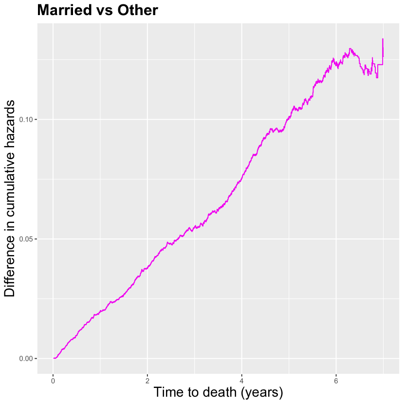
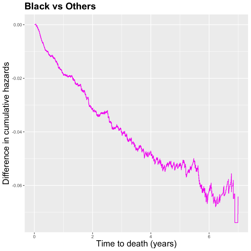
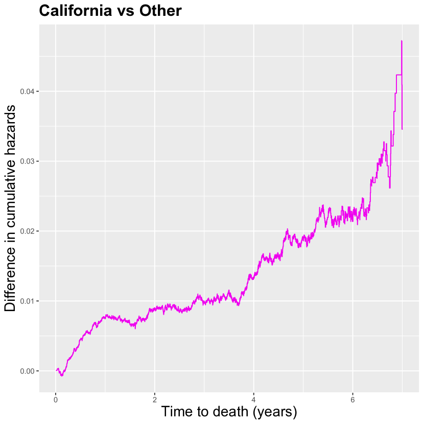
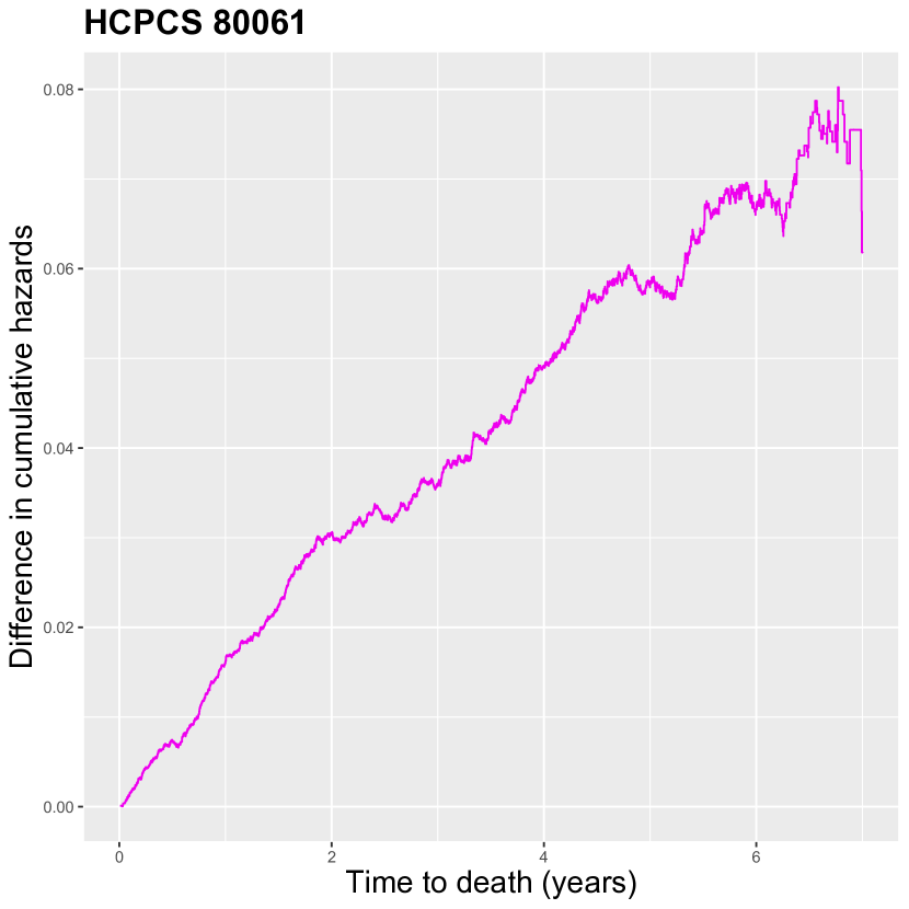
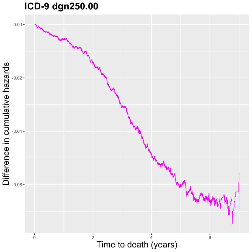
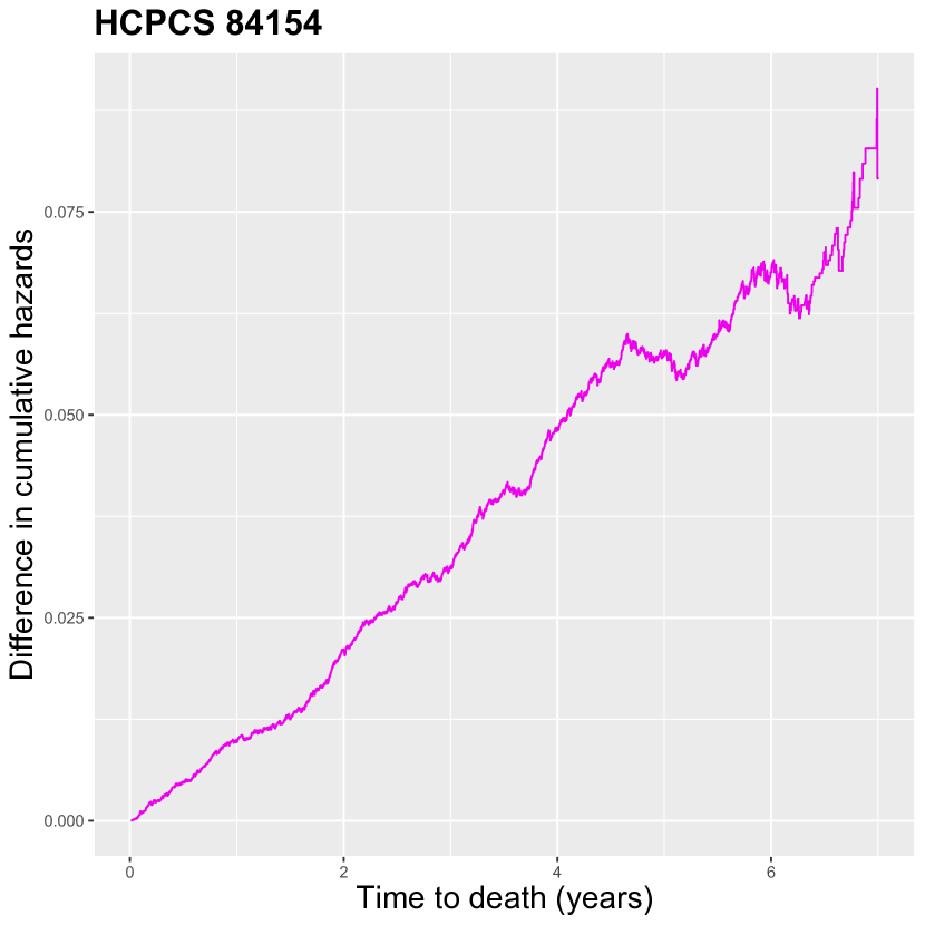
Figure 4: Difference between the cumulative hazard functions of groups defined by some dichotomous variables for the SEER-MEDICARE data.

Table 5: $R^{2}$ values for the SEER-Medicare data set. $R^{2}$ is computed on the full data set; $R^{2}_{adj}$ is the adjusted $R^{2}$ also computed on the full data set; $R^{2}_{out}$ is the out-of-sample $R^{2}$ computed on the test data set, with all parameters estimated from the training data set; and $R^{2}_{train}$ is computed only on the training data set.

Model	$R^{2}$	$R^{2}_{adj}$	$R^{2}_{out}$	$R^{2}_{train}$
Clinical	$0.048$	$0.048$	$0.053$	$0.051$
Clinical + Demo.	$0.270$	$0.270$	$0.271$	$0.261$
Clinical + Demo. + Claims	$0.373$	$0.370$	$0.388$	$0.379$

References

- Aalen [1980] Aalen OO. A model for non-parametric regression analysis of counting processes. Lecture Notes in Statistics - 2: Mathematical Statistics and Probability Theory 1980;p. 1–25.
- Aalen [1989] Aalen OO. A linear regression model for the analysis of life times. Statistics in medicine 1989;8(8):907–925.
- Martinussen and Vansteelandt [2013] Martinussen T, Vansteelandt S. On collapsibility and confounding bias in Cox and Aalen regression models. Lifetime Data Analysis 2013;19:279–296.
- Tchetgen Tchetgen et al. [2015] Tchetgen Tchetgen EJ, Walter S, Vansteelandt S, Martinussen T, Glymour M. Instrumental variable estimation in a survival context. Epidemiology 2015;26(3):402.
- Li et al. [2015] Li J, Fine J, Brookhart A. Instrumental variable additive hazards models. Biometrics 2015;71(1):122–130.
- Zheng et al. [2017] Zheng C, Dai R, Hari PN, Zhang MJ. Instrumental variable with competing risk model. Statistics in Medicine 2017;36:1240–1255.
- Brueckner et al. [2019] Brueckner M, Titman A, Jaki T. Instrumental variable estimation in semi-parametric additive hazards models. Biometrics 2019;75(1):110–120.
- Ying et al. [2019] Ying A, Xu R, Murphy J. Two-stage residual inclusion for survival data and competing risk- an instrumental variable approach with application to SEER-Medicare linked data. Statistics in Medicine 2019;38(1):125–138.
- Fosen et al. [2006] Fosen J, Ferkingstad E, Borgan Ø, Aalen OO. Dynamic path analysis?a new approach to analyzing time-dependent covariates. Lifetime data analysis 2006;12(2):143–167.
- Martinussen [2010] Martinussen T. Dynamic path analysis for event time data: large sample properties and inference. Lifetime data analysis 2010;16(1):85–101.
- Martinussen et al. [2011] Martinussen T, Vansteelandt S, Gerster M, Hjelmborg JvB. Estimation of direct effects for survival data by using the Aalen additive hazards model. Journal of the Royal Statistical Society: Series B (Statistical Methodology) 2011;73(5):773–788.
- VanderWeele [2013] VanderWeele TJ. Unmeasured confounding and hazard scales: sensitivity analysis for total, direct, and indirect effects. European journal of epidemiology 2013;28(2):113–117.
- Aalen et al. [2020] Aalen OO, Stensrud MJ, Didelez V, Daniel R, Røysland K, Strohmaier S. Time-dependent mediators in survival analysis: Modeling direct and indirect effects with the additive hazards model. Biometrical Journal 2020;62(3):532–549.
- Wang et al. [2017] Wang Y, Lee M, Liu P, Shi L, Yu Z, Awad YA, et al. Doubly robust additive hazards models to estimate effects of a continuous exposure on survival. Epidemiology 2017;28(6):771.
- Kang et al. [2018] Kang S, Lu W, Zhang J. On estimation of the optimal treatment regime with the additive hazards model. Statistica Sinica 2018;28(3):1539.
- Blomberg et al. [2019] Blomberg A, Wang Y, Di Q, Dominici F, Schwartz J, et al. Long-term effect of air pollution on hospital admissions among Medicare participants using a doubly robust additive hazards model (DRAHM). Environmental Epidemiology 2019;3:355.
- Dukes et al. [2019] Dukes O, Martinussen T, Tchetgen Tchetgen EJ, Vansteelandt S. On doubly robust estimation of the hazard difference. Biometrics 2019;75:100–019.
- Yuen and Burke [1997] Yuen KC, Burke MD. A test of fit for a semiparametric additive risk model. Biometrika 1997;84:631–639.
- Kim and Lee [1998] Kim J, Lee S. Two-sample goodness-of-fit tests for additive risk models with censored observations. Biometrika 1998;85:593–603.
- Scheike and Martinussen [2006] Scheike TH, Martinussen T. Dynamic Regression models for survival data. Springer, NY; 2006.
- O’Quigley and Xu [2012] O’Quigley J, Xu R. Explained variation and explained randomness for proportional hazards models. In: Handbook of Statistics in Clinical Oncology (3rd Ed.) Taylor & Francis Group, LLC; 2012. p. 487–503.
- Müller et al. [2008] Müller M, Döring A, Küchenhoff H, Lamina C, Malzahn D, Bickeböller H, et al. Quantifying the contribution of genetic variants for survival phenotypes. Genetic Epidemiology: The Official Publication of the International Genetic Epidemiology Society 2008;32(6):574–585.
- Hielscher et al. [2010] Hielscher T, Zucknick M, Werft W, Benner A. On the prognostic value of survival models with application to gene expression signatures. Statistics in Medicine 2010;29(7-8):818–829.
- Preseley et al. [2011] Preseley A, Tilahun A, Alonso A, Molenberghs G. An information-theoretic approach to surrogate-marker evaluation with failure time endpoints. Lifetime Data Analysis 2011;17:195–214.
- Kong et al. [2019] Kong E, Xia Y, Zhong W. Composite Coefficient of Determination and Its Application in Ultrahigh Dimensional Variable Screening. Journal of the American Statistical Association 2019;114(528):1740–1751.
- Kent and O’Quigley [1988] Kent JT, O’Quigley J. Measure of dependence for censored survival data. Biometrika 1988;75:525–534.
- Xu and O’Quigley [1999] Xu R, O’Quigley J. A type measure of dependence for proportional hazards models. Nonparametric Statistics 1999;12:83–107.
- O’Quigley et al. [2005] O’Quigley J, Xu R, Stare J. Explained randomness in proportional hazards models. Statistics in Medicine 2005;24:479–489.
- O’Quigley and Flandre [1994] O’Quigley J, Flandre P. Predictive capability of proportional hazards regression. Proceedings of the National Academy of Science USA 1994 March;91:2310–2314.
- Schemper and Kaider [1997] Schemper M, Kaider A. A new approach to estimate correlation coefficients in the presence of censoring and proportional hazards. Computational Statistics and Data Analysis 1997;23:467–476.
- Xu [2003] Xu R. Measuring explained variation in linear mixed effects models. Statistics in Medicine 2003;22:3527–3541.
- Honerkamp-Smith and Xu [2016] Honerkamp-Smith G, Xu R. Three measures of explained variation for correlated survival data under the proportional hazards mixed-effects model. Statistics in Medicine 2016;35(23):4153–4165.
- Chan et al. [2018] Chan PH, Xu R, Chambers CD. A Study of Measure under the Accelerated Failure Time Models. Communications in Statistics - Simulation and Computation 2018;47:380–391.
- Lin and Ying [1994] Lin DY, Ying Z. Semiparametric analysis of the additive risk model. Biometrika 1994;81:61–71.
- O’Quigley [2008] O’Quigley J. Proportional Hazards Regression. New York: Springer; 2008.
- Xu and O’Quigley [2000] Xu R, O’Quigley J. Estimating average regression effect under non-proportional hazards. Biostatistics 2000;1:423–439.
- Freireich et al. [1963] Freireich EJ, Gehan E, et al. The effect of 6-mercaptopurine on the duration of steroid-induced remissions in acute leukemia. Blood 1963;21:699–716.
- Cox and Oakes [1984] Cox DR, Oakes D. Analysis of Survival Data. Chapman and Hall; 1984.
- Hou et al. [2018] Hou J, Paravati A, Hou J, Xu R, Murphy J. High-dimensional variable selection and prediction under competing risks with application to SEER-Medicare linked data. Statistics in Medicine 2018;37:3486–3502.
- Riviere et al. [2019] Riviere P, Tokeshi C, Hou J, Nalawade V, Sarkar R, Paravati AJ, et al. Claims-based approach to predict cause-specific survival in men with prostate cancer. JCO clinical cancer informatics 2019;3:1–7.
- Ash and Shwartz [1999] Ash A, Shwartz M. : a useful measure of model performance when predicting a dichotomous outcome. Statistics in Medicine 1999;18:375–384.
- Chauvel and O’Quigley [2017] Chauvel C, O’Quigley J. Survival model construction guided by fit and predictive strength. Biometrics 2017;73(2):483–494.
- Flander and O’Quigley [2019] Flander P, O’Quigley J. Comparing Kaplan–Meier curves with delayed treatment effects: applications in immunotherapy trials. Journal of the Royal Statistical Society, Series C 2019;68:915–939.