Reconstructing gravitational wave signals from binary black hole mergers with minimal assumptions

Abstract

We present a systematic comparison of the binary black hole (BBH) signal waveform reconstructed by two independent and complementary approaches used in LIGO and Virgo source inference: a template-based analysis, and a morphology-independent analysis. We apply the two approaches to real events and to two sets of simulated observations made by adding simulated BBH signals to LIGO and Virgo detector noise. The first set is representative of the 10 BBH events in the first Gravitational Wave Transient Catalog (GWTC-1). The second set is constructed from a population of BBH systems with total mass and signal strength in the ranges that ground based detectors are typically sensitive. We find that the reconstruction quality of the GWTC-1 events is consistent with the results of both sets of simulated signals. We also demonstrate a simulated case where the presence of a mismodelled effect in the observed signal, namely higher order modes, can be identified through the morphology-independent analysis. This study is relevant for currently progressing and future observational runs by LIGO and Virgo.

I Introduction

The first Gravitational Wave Transient Catalog (GWTC-1) Abbott et al. (2019a) published by the LIGO and Virgo Collaboration Aasi et al. (2015); Acernese et al. (2015) includes signals from ten Binary Black Hole (BBH) sources and one binary neutron star (BNS) system. Along with neutron star-black hole (NSBH) binaries, these sources are referred to as compact binary coalescences (CBCs). Ground based detectors are most sensitive to transient signals from CBC systems with total mass $M_{T}$ in the stellar mass range ($10M_{\odot}\lesssim M_{T}\lesssim 100M_{\odot}$). The gravitational wave (GW) emission becomes loudest in the sensitive frequency band ($20-1000$ Hz) Harry (2010) milliseconds to minutes before the merger, just as the GW emission reaches peak amplitude.

There are two main types of transient GW analysis: targeted template-based matched-filter “CBC” analyses which use physically-motivated waveform models Allen et al. (2012), and morphology-independent “burst” analyses Anderson et al. (2001); Andersson et al. (2013). The models used in CBC analyses Usman et al. (2016); Messick et al. (2017) are semi-analytical solutions of General Relativity (GR) that combine aspects of analytical post-Newtonian theory to model the inspiral, and Numerical Relativity (NR) Pretorius (2005); Campanelli et al. (2006); Baker et al. (2006) to capture the highly non-linear late inspiral and merger phases Bohé et al. (2017). The CBC templates account for the dominant $(l,|m|)=(2,2)$ mode in the spherical harmonic formulation of GW radiation. Burst analyses model GWs as a superposition of a number of suitable basis functions parameterized by observable quantities such as amplitude and frequency Klimenko et al. (2008); Lynch et al. (2017). The inexact match of the basis functions with underlying GW signals results in generally lower intrinsic sensitivity than targeted CBC searches but the larger number of degrees of freedom allows for the recovery of un-modelled waveform phenomenology and, potentially, new physics. Burst methods are also used to search for GW signals from sources such as supernovae New (2003) and the post-merger phase of binary neutron star coalescence, where the physics is too uncertain to develop a sufficiently robust matched-filter template Abbott et al. (2019b, 2017a); Chatziioannou et al. (2017); Torres-Rivas et al. (2019).

Following the detection of a GW signal in the data, Parameter Estimation (PE) analysis is performed by LALInference Veitch et al. (2015), which uses CBC models to sample the posterior probability distribution (PDF) of the physical parameters, e.g. masses and spins, using stochastic samplers such as Makov Chain Monte Carlo (MCMC)Gilks et al. (1995); Metropolis et al. (1953); Geman and Geman (1987); Rover et al. (2006); Christensen and Meyer (2001); Rover et al. (2007); Raymond et al. (2010) and Nested Sampling Skilling et al. (2006); Veitch and Vecchio (2010). The resulting PDF is used in studies including formation scenarios, rates and tests of GR.

A “Burst” PE analysis is performed by BayesWave Cornish and Littenberg (2015); Littenberg and Cornish (2015). BayesWave models the signal waveform as a sum of Morlet Gabor wavelets Morlet et al. (1982) and uses a trans-dimensional Reversible Jump Markov Chain Monte Carlo (RJMCMC) to sample the parameters as well as the number of the wavelets Green (1995). BayesWave will reconstruct any feature in the data that is coherent across the detector network if the feature is loud enough compared to the background noise. This makes the wavelet model flexible enough to fit a wide range of signal morphologies. For the case of BBH signals, it is most sensitive to times close to the merger where the amplitude peaks.

Wavelets and CBC waveforms provide complementary means to study GW signals. Fig. 1 shows the waveform reconstructions and their 90% credible intervals given by LALInference using the precessing, dominant mode approximant IMRPhenomPv2 Hannam et al. (2014) from the Phenom waveform family, and by BayesWave for GW150914 Abbott et al. (2016a). Waveform reconstruction plots that similarly illustrate the agreement between CBC and burst reconstructions and have been used in works on GW150914 Abbott et al. (2016b), GW170104 Abbott et al. (2017b), GW170814 Abbott et al. (2017c), GW170729 Chatziioannou et al. (2019a), and GWTC-1 Abbott et al. (2019a). Comparing wavelet-based and waveform-based signal reconstructions serves as a consistency check for the signal morphology. A general feature of these plots is that the reconstructions agree at times close to the merger where the signal is strong, but do not necessarily have to agree where the signal is weak. This is because accuracy of BayesWave of reconstruction a feature depends on the loudness of the feature. We also note that the BayesWave credible intervals are broader than the LALInference credible intervals since the former allows for more flexibility in the waveform morphology.

Reference Abbott et al. (2016b) studies the agreement between a set of simulated GW signals injected into real data and the reconstructions obtained using BayesWave. A related test of signal consistency is the residuals test which uses BayesWave to analyze the residual obtained by subtracting from the detector data the reconstructed CBC signal. The result is then compared to the same analysis on surrounding noise to quantify the evidence for any residual excess. This test has been employed in Abbott et al. (2016c, 2019c, 2017b).

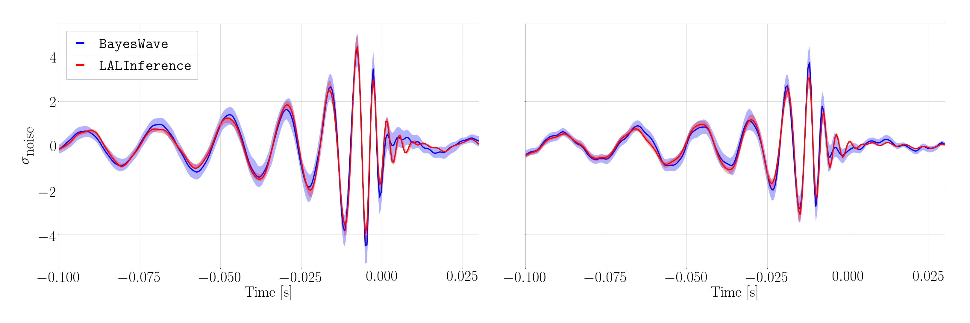
Figure 1: LAInference IMRPhenomPv2 (red) Hannam et al. (2014) and BayesWave (blue) reconstructions of GW150914 Abbott et al. (2016a) using publicly released data from GWTC-1 LIGO Scientific (2018). The left and right panels respectively show the waveform in LIGO Hanford and LIGO Livingston. The x-axis represents the time in seconds before the coalescence. The y axis represents the strain amplitude whitened using a filter which is the inverse amplitude spectral density (ASD). The units are in multiples of the standard deviation of the noise.

This paper presents a systematic performance comparison of the two algorithms applied to BBH systems. It provides the context in which the reconstructions of future gravitational wave events can be evaluated, which is particularly timely given the approximately weekly BBH detections during the third LIGO and Virgo observing run. Instead of qualitative plot comparisons, we use a quantitative comparison metric that is the overlap, which is the noise weighted inner product of waveforms reconstructed by each algorithm. Simulated BBH GW signals are added to detector noise from the LIGO and Virgo detectors. These “injections” are then analyzed using LALInference and BayesWave. We perform two types of injections: in the first, we inject populations of signals whose physical parameters are drawn from the posterior probability distributions inferred from GWTC-1 events Vallisneri et al. (2015). We also analyze a population of BBH injections whose masses are drawn uniformly from ranges which explore ground based detector sensitivities and signal durations.

We find that the waveform reconstructions of events in the GWTC-1 catalog are consistent, within 90% credibility, with expectations based on our simulations of similar signals. Analysis of signals drawn from across the mass spectrum also illustrates that BayesWave performs significantly better for higher mass systems while the template-based LALInference reconstructions are relatively insensitive to the mass ranges explored in this study. This is to be expected, since shorter-duration with fewer cycles most closely resemble the wavelet basis used by BayesWave, bringing the analysis closer to matched-filtering.

There remain known physical effects, such as precession, orbital eccentricity, extreme mass ratios which have historically been difficult to incorporate into analytical models for BBH GW waveforms. Less certain effects, such as deviations from GR, are still more difficult to model. With developments in technology such as LIGO A+ Barsotti et al. (2018), and third generation detectors such as the Einstein Telescope and Voyager Punturo et al. (2010); Collaboration (2016), the network of ground based detectors will reach sensitivities where these effects will in principle, be loud enough to cause significant disagreement between the reconstrucions given by the CBC and model-independent analyses. As an illustration of such a scenario, we analyze a numerical relativity waveform from the Georgia Tech catalogJani et al. (2016). In this system, Higher Order Modes (HOMs) contribute a substantial fraction of the total signal-to-noise ratio Calderon Bustillo et al. (2017). While there now exist waveform templates which accurately model HOMs London et al. (2018); Cotesta et al. (2018), analysis of this signal with a more rudimentary waveform model Hannam et al. (2014) is a convenient way to highlight what a disparity in LALInference and BayesWave reconstructions would look like. We analyze the performance of LALInference and BayesWave when this waveform is injected into data and find that the latter is able to reconstruct the waveform more accurately due to its flexibility.

Section II delves into the details of LALInference and BayesWave, their waveform models, sampling techniques, and calculation of the overlap. Section III describes the set of injections in detail. Section IV discusses the results and inferences. Section V briefly discusses the performace comparison of the two algorithms when HOMs are included in the injection. Section VI concludes the paper and discusses possible future work.

II Methodology

The properties of a detected signal are inferred by modeling the detector data $\mathbf{d}$ with the parameterized waveform $\mathbf{h}(\theta)$. The boldface here is to emphasize that $\mathbf{d}$ and $\mathbf{h}$ represent quantities in multiple detectors. Here $\theta=\{\theta_{1},\theta_{2},...,\theta_{N}\}$ represents a point the parameter space of the underlying CBC system in the case of LALInference such as masses and spins, or the parameter space of wavelets in the case of BayesWave such as the central frequency, amplitude and number of wavelets. The data $\mathbf{d}$ are assumed to be a time series that contains the true GW signal, plus additive stationary Gaussian noise characterized by the one-sided noise Power Spectral Density (PSD) $S_{n}(f)$. We are interested in sampling the posterior probability distribution function of $\mathbf{h}$ given $\mathbf{d}$. Accoriding to Bayes’ theorem Bayes (1763); Jaynes (1996):

$$p(\mathbf{h}|\mathbf{d})=\frac{p(\mathbf{h})p(\mathbf{d}|\mathbf{d})}{p(\mathbf{d})},$$ (1)

where $p(\mathbf{h})$ is the prior knowledge about the system. $p(\mathbf{d}|\mathbf{h})$ is the likelihood function, the probability of obtaining data $\mathbf{d}$ given the signal $\mathbf{h}$:

$$p(\mathbf{d}|\mathbf{h})\propto\exp\left(-\frac{1}{2}\langle\mathbf{d}-\mathbf{h}|\mathbf{d}-\mathbf{h}\rangle\right),$$ (2)

where $\langle\cdot|\cdot\rangle$ on quantities with boldface indicates the noise weighed inner product over the network of detectors given by:

$$\langle\mathbf{a}|\mathbf{b}\rangle=\sum_{i}^{n}\langle a^{i}|b^{i}\rangle,$$ (3)

here $i$ sums over all $n$ detectors in the network, and $\langle a^{i}|b^{i}\rangle$ is the inner product in an individual detector defined in as

$$\langle a^{i}|b^{i}\rangle\equiv 4\Re\int_{0}^{\infty}\frac{\tilde{a}^{i}(f)\tilde{b}^{i*}(f)}{S_{n}^{i}(f)}df,$$ (4)

$\tilde{a}^{i}(f)$ is the Fourier transform of time series $a^{i}$, and the superscript $*$ denotes the complex conjugate. $S_{n}^{i}(f)$ is the PSD of the $i^{\textrm{th}}$ detector. Dividing by the PSD effectively reweights the integral towards frequencies where the detectors are most sensitive. The optimal Signal to Noise Ratio (SNR) is defined as

$$\rho=\sqrt{\langle\mathbf{d}|\mathbf{d}\rangle},$$ (5)

and is often used as a figure of merit for the strength of the signal in the detector.

The signal in the $i^{th}$ detector, $h^{i}$, is obtained by projecting the “plus” ($h_{+}$) and “cross” ($h_{\times}$) using the sky-location dependent antenna pattern functions $F_{+}^{i}$ and $F_{\times}^{i}$:

$$h^{i}=F^{i}_{+}(\theta,\phi,\psi)\,h^{i}_{+}+F^{i}_{\times}(\theta,\phi,\psi)\,h^{i}_{\times}$$ (6)

The computational cost of estimating the likelihood function using deterministic methods is high, as the number of valuations required to explore the parameter space on a fixed grid grows exponentially with the number of dimensions. This can become prohibitively expensive beyond a few dimensions. Therefore, sampling-based methods such as Markov Chain Monte Carlo (MCMC) Gilks et al. (1995); Metropolis et al. (1953); Geman and Geman (1987); Rover et al. (2006); Christensen and Meyer (2001); Rover et al. (2007); Raymond et al. (2010) and Nested Sampling Skilling et al. (2006); Veitch and Vecchio (2010) are often used.

II.1 LALInference

LALInference Veitch et al. (2015) models the signal $\mathbf{d}$ in the detector data as a CBC GW signal described by GR. It uses analytical or semi-analytical approximants to construct the signal waveform. To sample the parameter space it uses two main techniques: Nested Sampling Skilling et al. (2006); Veitch and Vecchio (2010) and MCMC Gilks et al. (1995); Metropolis et al. (1953); Geman and Geman (1987); Rover et al. (2006); Christensen and Meyer (2001); Rover et al. (2007); Raymond et al. (2010).

The parameter samples of GWTC-1 use the precessing, dominant mode approximants from the two main families: IMRPhenomPv2 Hannam et al. (2014) from the Phenom family, and SEOBNRv3 Taracchini et al. (2014); Pan et al. (2014) from the EOB-NR family. For this paper we use the IMRPhenomPv2 samples to perform injections, and use a reduced order quadrature (ROQ) Smith et al. (2016) of IMRPhenomPv2 to compute the likelihood while analyzing with LALInference. The ROQ reduces the computational cost of parameter estimation by reducing redundant computations. We do not use the SEOBNRv3 approximant for recovery as it is computationally more expensive. Studies such as Abbott et al. (2019a) have shown that IMRPhenomPv2 and SEOBNRv3 samples for BBH systems in GWTC-1 broadly agree with each other.

II.2 BayesWave

BayesWave Cornish and Littenberg (2015); Littenberg and Cornish (2015) models the signal $\mathbf{d}$ in the detectors as a summation of Morlet Gabor wavelets, the number and parameters of which are marginalized over using the reversible jump markov chain monte carlo (RJMCMC) sampler.

The signal model consists of a variable number of wavelets, where each wavelet, $\Psi$, is described by five parameters: the central time $t_{0}$, the central frequency $f_{0}$, the quality factor $Q$, the amplitude $A$, and the phase offset $\phi_{0}$. In the frequency domain, the wavelet is given by

$$\widetilde{\Psi}(f;A,Q,f_{0},t_{0},\phi_{0})=\\ \frac{\sqrt{\pi}A\tau}{2}e^{-\pi^{2}\tau^{2}(f-f_{0})^{2}}e^{i(\phi_{0}+2\pi(f-f_{0})t_{0})},$$ (7)

where $\tau=Q/2\pi f_{0}$ and and $\tilde{\cdot}$ represents the frequency domain version of any quantity. Assuming an elliptically polarized GW signal, the plus component ($h_{+}$) of the GW strain is given by $\widetilde{h}_{+}=\sum_{j=0}^{N}\Psi_{j}$, where $N$ is the number of wavelets that describe the signal model. The cross component ($h_{\times}$) is given by $\widetilde{h}_{\times}=ie\widetilde{h}_{+}$, where $e$ is the ellipticity paramter which is also sampled over. Details of the wavelet model used in BayesWave can be found in Cornish and Littenberg (2015). A generalization of the wavelet model is the chirplet model which includes a time dependent frequency component Millhouse et al. (2018).

Since we are testing the infrastructure as employed by past LIGO and Virgo Collaboration papers, we limit our analysis to the wavelet model. Past studies such as Chatziioannou et al. (2019a) have shown that the wavelet and chirplet models have similar levels of agreement with CBC waveforms for the observed BBH systems. We also limit ourselves to the frequency independent ellipticity ($e$) assumption. BayesWave was initially developed using the elliptical polarization assumption since the early era of GW astronomy had only two nearly-aligned LIGO detectors which resulted in poor polarization sensitivity. Recent works such as Abbott et al. (2020) show that HOMs are measurable with the current detector network sensitivities and it is important to relax the ellipticity constraint, where the parameters of $\widetilde{h}_{+}$ and $\widetilde{h}_{\times}$ are independently sampled. At the time of preparing this work, development towards this independent polarization model is complete and has been demonstrated to work. It will be discussed in future works.

II.3 Overlap

To quantify the agreement between LALInference and BayesWave, we use point estimates of the signal waveform from each. In the case of LALInference, we use the posterior sample for which the likelihood function described in Eq 2 is maximum, which we will call the maximum likelihood LALInference waveform (MLW). We caution that this is a good approximation of, but not necessarily, the true maximum, as LALInference is a posterior distribution inferring algorithm, rather than a peak finding algorithm. For BayesWave we use the estimate obtained by taking the median of the waveform value at every time index from the whole set of samples. We call this the median BayesWave waveform (MBW). We do not use the maximum likelihood BayesWave waveform since unlike CBC waveforms, the wavelets are “nuisance parameters” that do not have any physical meaning themselves. Instead it is the fit waveform that is fundamentally of interest. The MBW is a collective estimate across samples that is stable because it is relatively immune to the stochastic fluctuations of the variable dimensional sampler.

We quantify the agreement between the MLW ($\mathbf{h}_{\textrm{LI}}$) and the MBW ($\mathbf{h}_{\textrm{BW}}$) by computing the overlap over the network of detectors Apostolatos (1995).

$${\cal{O}}_{\textrm{B,L}}\equiv\frac{\langle\mathbf{h}_{\textrm{LI}}|\mathbf{h}_{\textrm{BW}}\rangle}{\sqrt{\langle\mathbf{h}_{\textrm{LI}}|\mathbf{h}_{\textrm{LI}}\rangle\langle\mathbf{h}_{\textrm{BW}}|\mathbf{h}_{\textrm{BW}}\rangle}},$$ (8)

We use the parameterized version given by the BayesLine Littenberg and Cornish (2015) algorithm which is a fully integrated in BayesWave. BayesLine models the PSD with two components: a cubic spline to fit the broad band noise, and a sum of Lorentzians to fit the narrow band spectral lines. The number and location of Lorentzians and cubic spline control plots are again determined with a RJMCMC. This PSD estimate is completely determined by the data segment under analysis, which is more robust to slowly varying non-stationary noise compared to off-source spectral estimation using, e.g., Welch’s method. Details of the BayesLine algorithm can be found in Littenberg and Cornish (2015), and an in-depth study describing its merits over using the Welch’s method can be found in Chatziioannou et al. (2019b).

III Injections

To understand the variation of the overlap $\langle\mathbf{h}_{\textrm{LI}}|\mathbf{h}_{\textrm{BW}}\rangle$ as a function of the system properties, we run LALInference and BayesWave on simulated GW signals added to noise from the LIGO and Virgo detectors. A simulated signal that is added to noise is also called an “injection”. To perform injections, the instrument noise from the LIGO and Virgo detectors is combined with the simulated CBC waveform to make the simulated observation data stream $\mathbf{d}$. This is then analyzed by the BayesLine algorithm which computes the median PSD, $S_{n}(f)$, that is used in the likelihood computations described in Equation 2. $S_{n}(f)$ and $\mathbf{d}$ are then fed into LALInference and BayesWave for analysis. This is exactly the same procedure as is used in LIGO and Virgo data offline PE follow up analyses on actual GW event detections. We compute the overlap between $\mathbf{h}_{\textrm{LI}}$ and $\mathbf{h}_{\textrm{BW}}$ using Eq. 8.

We apply the above analysis to two types of injections. The first type, “GWTC-1 injections” are injections of signals from systems whose parameters are drawn from the posterior distribution samples of GW events in GWTC-1. The purpose of these injections is to establish an expectation of the overlap for a each event in GWTC-1, which we then use to compare with the overlap on the actual event observation data. The second type, referred to as “Population injections”, are injections of signals from systems with total mass $M_{T}$ in the range range $10M_{\odot}$ to $120M_{\odot}$. These help us establish typical trends in the overlap over a broad range of systems.

The two types of injections yield complimentary inferences. GWTC-1 injections focus on CBC systems specific to events in GWTC-1 and are designed to gauge the reconstruction performance of the catalog, whereas the population injections are designed to infer the trends in the overlap over the range of systems that we expect to detect in ground based detectors.

III.1 Reconstruction of Detected Signals

To test the reconstruction fidelity for real events, we design a set of $500$ injections, $50$ for each of the $10$ GWTC-1 events. The parameters of these injections are sampled from their measured IMRPhenomPv2 Hannam et al. (2014) posterior probability density functions. We use the LALInference posterior samples files available on the Gravitational Wave Open Science Center (GWOSC) Vallisneri et al. (2015) and for each of the above injections, compute the “offsource” overlap ($\cal{O}_{\textrm{OFS}}$ $=\langle\mathbf{h}_{\textrm{LI}}|\mathbf{h}_{\textrm{BW}}\rangle$). We then compare the distribution resulting from these $50$ $\cal{O}_{\textrm{OFS}}$ values with the “onsource” overlap ($\cal{O}_{\textrm{ONS}}$ $=\langle\mathbf{h}_{\textrm{LI}}|\mathbf{h}_{\textrm{BW}}\rangle$) obtained from the data containing the real event.

Since the parameters of these events are mostly consistent with nearly equal mass, spin-aligned systems with little to no evidence for precession, we expect the $\cal{O}_{\textrm{ONS}}$ value(s) to be no worse than the $\cal{O}_{\textrm{OFS}}$ overlaps(s).

We quantify this consistency using the p-value which we define as the fraction of $\cal{O}_{\textrm{OFS}}$ that are less than or equal to $\cal{O}_{\textrm{ONS}}$, i.e, $p\coloneqq P(\textrm{O}_{\textrm{OFS}}\leq\textrm{O}_{\textrm{ONS}})$. A smaller p-value indicates a smaller chance that the onsource reconstruction performance is consistent with what we expect. This could point to features in the onsource data that corrupt the reconstruction performance. These artifacts could be astrophysical or terrestrial in nature.

III.2 Reconstruction Fidelity

Past studies have shown that the agreement between burst and CBC waveforms is most sensitive to the total mass $M_{T}$ of the GW source and the SNR of the GW signal, and monotically increases for both these quantities Abbott et al. (2016b). To systematically study the trends in the overlap as a function of these quantities, we analyze injections of a population of IMRPhenomPv2 waveforms using LALInference and BayesWave. We inject into noise from the second observing run of the LIGO detectors Vallisneri et al. (2015). We divide these “population injections” into four different subsets based on their total mass $M_{T}$: (i) $10\,M_{\odot}<M_{T}<30\,M_{\odot}$, (ii) $30\,M_{\odot}<M_{T}<60\,M_{\odot}$, (iii) $60\,M_{\odot}<M_{T}<90\,M_{\odot}$, (iv) $90\,M_{\odot}<M_{T}<120\,M_{\odot}$, the typical mass ranges we expect to observe in ground based detectors. The mass ratios, spins, orientations and sky locations were distributed uniformly. For each of the mass ranges, we created five population sets of SNRs: $10$, $20$, $30$, $60$, $90$. To strike a balance between compuational cost and number of sample points, we perform $50$ injections per SNR range per mass range, for a total of 1000 injections.

IV Results

IV.1 GWTC-1 Injections

We plot $\cal{O}_{\textrm{ONS}}$ as a function of $\cal{O}_{\textrm{OFS}}$ for each BBH in GWTC-1 in Fig. 2. Due to variations in the parameter posteriors and/or noise properties, the distribution of O${}_{\textrm{OFS}}$ has a spread. The overlaid diagonal line here ($y=x$) represents the null hypothesis that the $\cal{O}_{\textrm{OFS}}$ and $\cal{O}_{\textrm{ONS}}$ are equal. Dots represent the median and the horizontal error bars are the $90\%$ credible intervals of the $\cal{O}_{\textrm{OFS}}$ distributions. From Fig. 2, we find that all events are consistent with $y=x$ within $90\%$ credibility. The median of $\cal{O}_{\textrm{OFS}}$ decreases and its spread increases with decreasing SNR and $M_{T}$ of the event. For example, GW150914 with an SNR $\sim 24$ and $M_{T}\sim 65M_{\odot}$ has a larger $\cal{O}_{\textrm{OFS}}$ median and a smaller spread compared to GW170823 which has a similar $M_{T}$ but has SNR $\sim 11$. Similarly, GW170729, with a $M_{T}\sim 84M_{\odot}$ and SNR $\sim 10$ has a larger median value and a smaller spread compared to GW151012 with similar SNR but $M_{T}\sim 27M_{\odot}$.

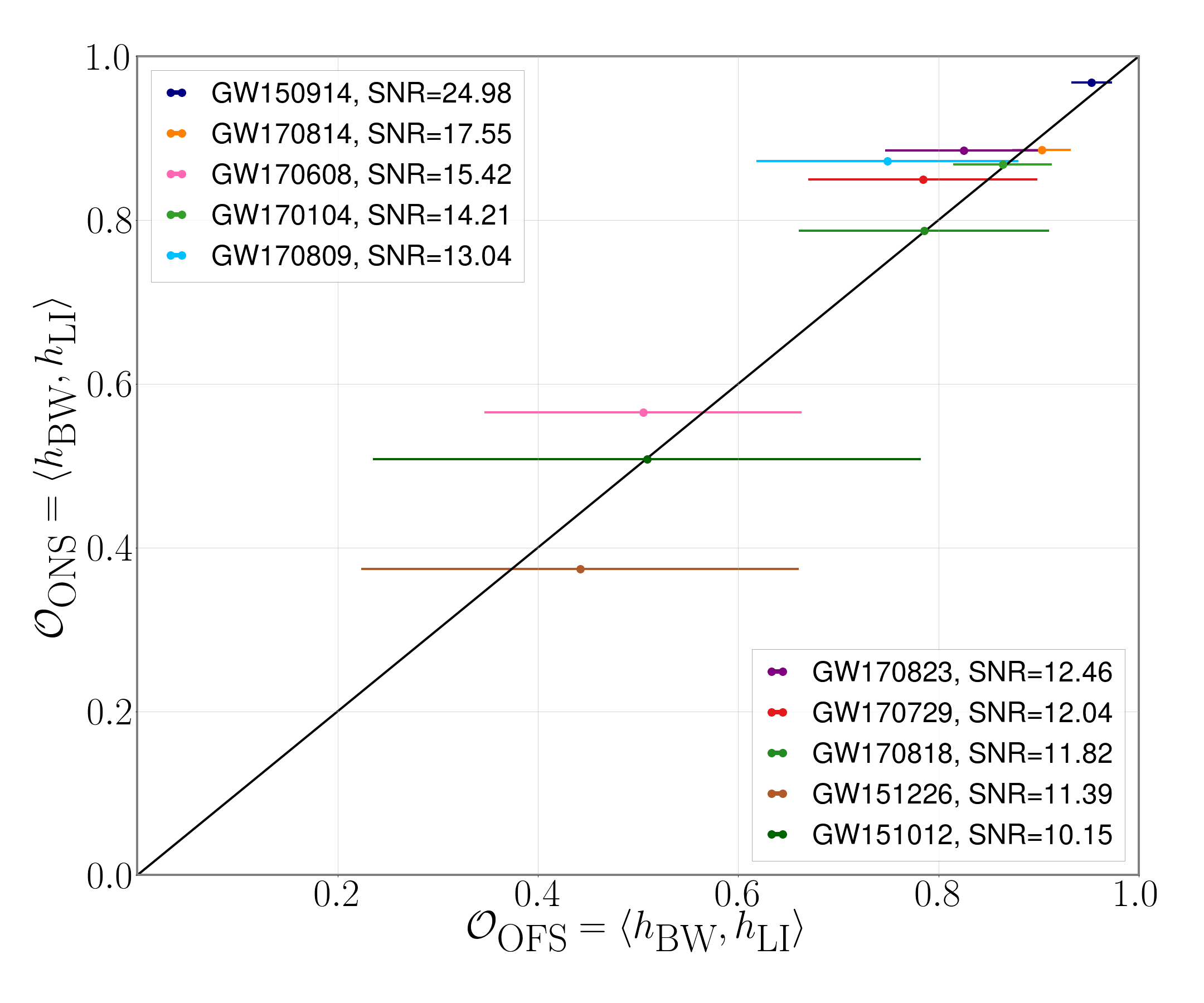
Figure 2: Onsource overlap (y axis) plotted against the median offsource overlap (x axis) for each of the GWTC-1 events. The horizontal error bars are the $90\%$ credible intervals in the overlap. The diagonal black line is $y=x$.

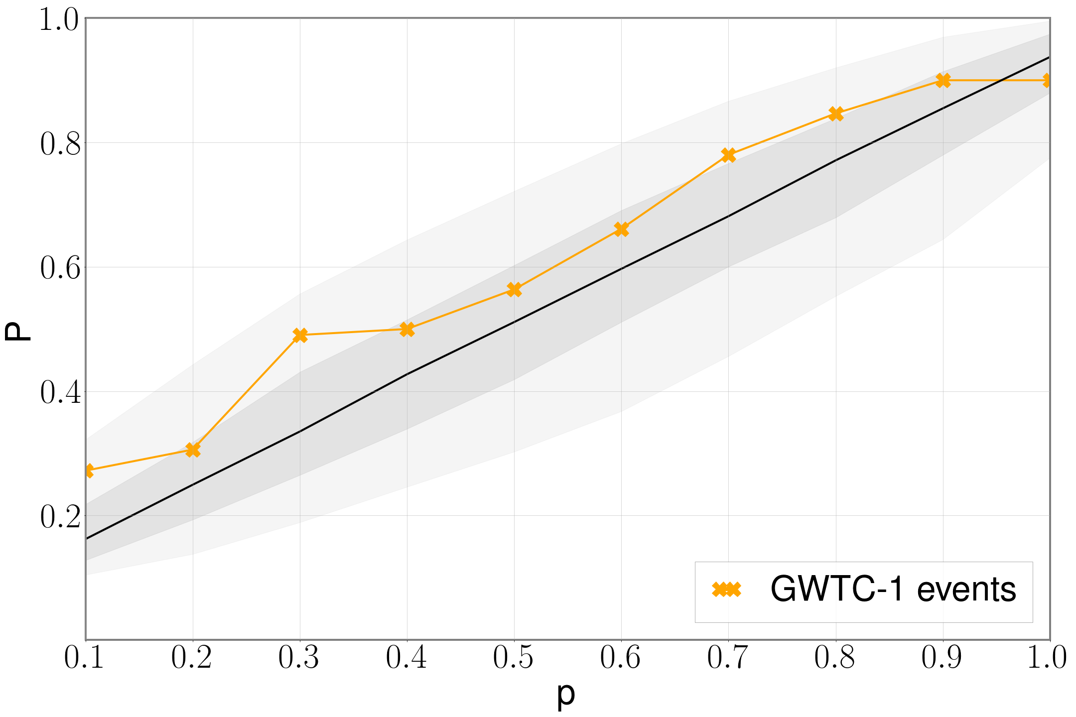
Figure 3: p-values (P) of GWTC-1 events (orange) plotted against the cumulative fraction events (p), along with the null hypothesis (black) and the 50% and 90% credible intervals (shaded regions).

We compute the p-values and record them in Table 1. We find that the p-values are broadly consistent with the null hypothesis that the onsource performance is no worse than the offsource performance. The lowest p-value that we compute is for GW151226 at $0.27$. Assuming the null hypothesis to be true for all events, we expect the p-values to be uniformly distributed between $0$ and $1$. We follow a procedure similar to Abbott et al. (2019c), and use the Fisher’s method Mosteller and Fisher (1948) to compute the meta analysis p-value (p${}_{\textrm{meta}}$) of the distribution of p-values. A p${}_{\textrm{meta}}$ close to $1$ indicates higher evidence for the meta null hypothesis, and a p${}_{\textrm{meta}}$ less than $0.05$ is considered low enough to reject the meta null hypothesis. We obtain a p${}_{\textrm{meta}}=0.95$ which indicates that there is no evidence for an aberrant behavior in the onsource reconstruction performance as compared to the offsource injections.

We also plot the p-values against the cumulative fraction of events in Fig. 3. The black line represents the null hypothesis that the p-values are uniformly distributed, and the shaded bands represent the 50% and 90% credible intervals. The orange curve is consistent with the black line within the 90% credible interval. Overall, this means that the agreement between burst and CBC reconstructions for GWTC-1 events is statistically consistent with what we expect.

Event	p-value
GW150914	$0.90$
GW151012	$0.49$
GW151226	$0.27$
GW170104	$0.56$
GW170608	$0.66$
GW170729	$0.78$
GW170809	$0.90$
GW170814	$0.30$
GW170818	$0.50$
GW170823	$0.84$

Table 1: p-values of GWTC-1 events computed by comparing the onsource overlap of $\langle\mathbf{h}_{\textrm{LI}},\mathbf{h}_{\textrm{BW}}\rangle$ versus the offsource distribution of the same

IV.2 Population Injections

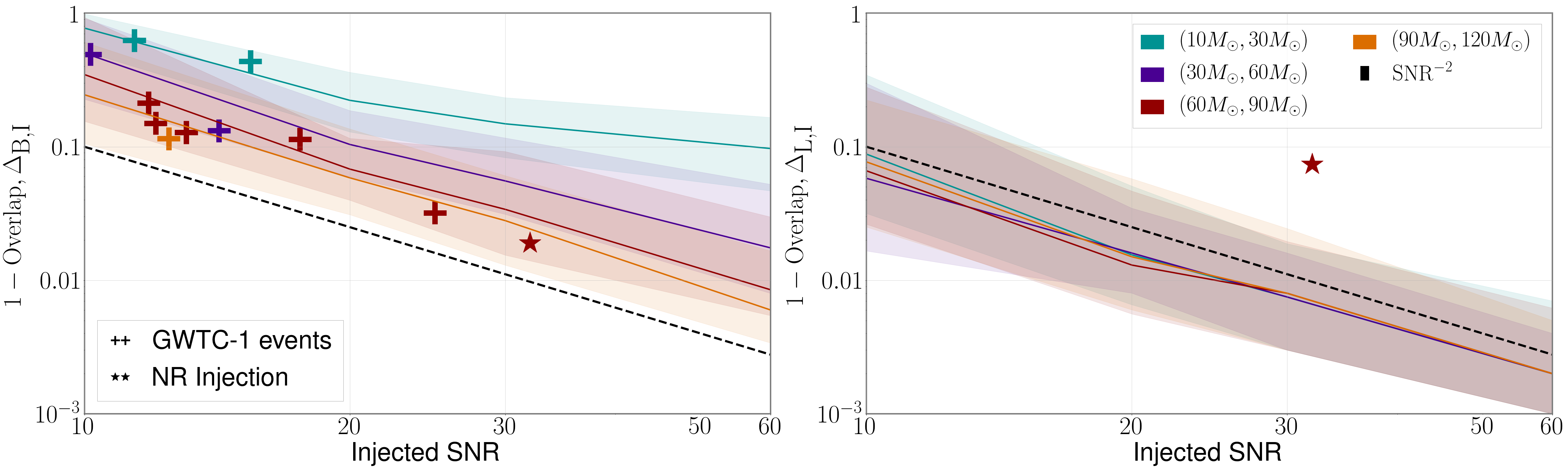
Figure 4: Medians (solid lines) and 90$\%$ uncertainty bands (shaded regions) of $\Delta_{\textrm{B,I}}$ (left) and $\Delta_{\textrm{L,I}}$(right) against the SNR ($\sqrt{\langle\mathbf{h}_{\textrm{INJ}},\mathbf{h}_{\textrm{INJ}}\rangle}$) of the CBC signal colored by the total mass ranges $M_{T}$. The black dashed-dot line represents the curve $1/\textrm{SNR{}}^{2}$ which is the expected variation of $\Delta_{\textrm{B,I}}$ and $\Delta_{\textrm{L,I}}$ for a signal. The overlaid “$+$” markers indicate the onsource values of $\Delta_{\textrm{B,L}}$ plotted against the SNR of the $\mathbf{h}_{\textrm{LI}}$ waveforms for each of the GWTC-1 events, and are colored by the to $M_{T}$ of the $\mathbf{h}_{\textrm{LI}}$ waveform. The overlaid “$*$” markers indicate the values inferred from the NR injection described in Section V.

For each $M_{T}$ range and SNR pair, we compute of overlaps between $\mathbf{h}_{\textrm{BW}}$ and the injected CBC signal, $\mathbf{h}_{\textrm{INJ}}$ ($\cal{O}_{\textrm{B,I}}$), and the overlap between the $\mathbf{h}_{\textrm{LI}}$ and $\mathbf{h}_{\textrm{INJ}}$ ($\cal{O}_{\textrm{L,I}}$). As reconstruction performance improves, the overlaps become closer to $1$. For ease of visual interpretation, we define $\Delta=1-\cal{O}$, where $\cal{O}$ is the overlap, and we use the same subscripts as for the overlap. $\Delta$ quantifies the disagreement between two waveforms. For each $M_{T}$ range, we obtain $\Delta$ distributions. We then plot the medians and 90$\%$ confidence intervals of these distributions as a function of the SNR in Fig. 4.

We see that at low SNRs, $\Delta_{\textrm{B,I}}$, where the subscripts “B” and “I” respectively represent BayesWave and the injection, starts off high as BayesWave is unable to recover the full signal. This is even more pronounced in systems with lower $M_{T}$ since the signal waveform is longer and the SNR is spread over a longer duration. We also see that at a particular SNR, $\Delta_{\textrm{B,I}}$ decreases with increasing $M_{T}$, since the signal waveform gets increasingly shorter and is more compactly represented with the wavelet model. $\Delta_{\textrm{B,I}}$ falls steadily as the SNR increases. On the other hand, $\Delta_{\textrm{L,I}}$, where subscripts “L” and “I” represent LALInference and the injection, is less than $0.2$, even for low SNRs, as LALInference can reconstruct the CBC signal morphology better than BayesWave at lower SNR. This is expected, since LALInference is using templates which predict the signal over the entire observing band. BayesWave however, can only reconstruct high amplitude features in the data. $\Delta_{\textrm{B,I}}$ becomes smaller as $M_{T}$ and SNR increase, and BayesWave is able to reconstruct more and more parts of the signal. Past studies have shown that we expect $\Delta_{\textrm{B,I}}$ and $\Delta_{\textrm{L,I}}$ to vary as $\propto 1/\textrm{SNR{}}^{2}$ Becsy et al. (2017). We plot this curve and up to a constant scaling factor, we see that the slopes of the reconstructions follow this relationship to a large extent.

As an additional test of consistency, we overlay the values obtained from the onsource results of the GWTC-1 events in Fig. 4. Specifically, we plot the $\Delta_{\textrm{B,L}}$, the complement of the overlap between $\mathbf{h}_{\textrm{BW}}$ and $\mathbf{h}_{\textrm{LI}}$ against the SNR of the $\mathbf{h}_{\textrm{LI}}$ given by $\sqrt{\langle\mathbf{h}_{\textrm{LI}},\mathbf{h}_{\textrm{LI}}\rangle}$, using $\mathbf{h}_{\textrm{LI}}$ as a proxy for the true waveform. We justify this approximation by noting from Fig. 4 that $\Delta_{\textrm{L,I}}$ is less than $0.1$ which is an order a magnitude smaller than $\Delta_{\textrm{B,I}}$. The markers are colored according to the color scheme of the $M_{T}$ parameter as shown in Fig. 4. We find that the $\Delta_{\textrm{B,L}}$ values fall within the bounds obtained from the population injections, which agrees with the inferences we drew in Section IV.1.

V Detecting deviations

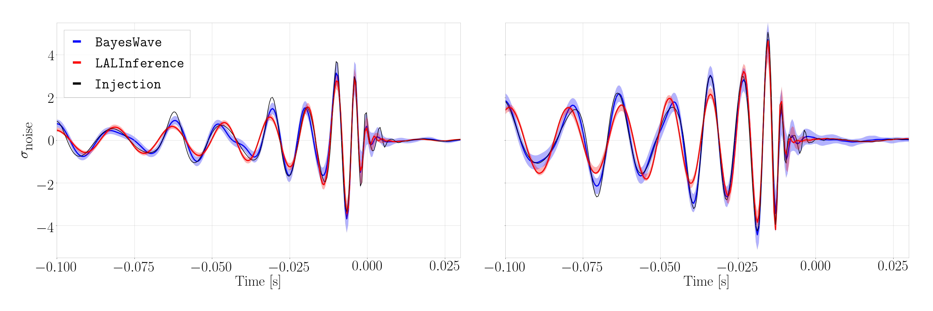
Figure 5: LALInference(red), BayesWave (blue), and the injected waveform (black) for the injection analysis performed using the Georgia Tech NR waveform GT0745. The plotting conventions are similar to Fig. 1. Note the disagreement between $\mathbf{h}_{\textrm{LI}}$ and $\mathbf{h}_{\textrm{BW}}$, especially before $-0.4$ seconds.

Our analysis so far has been focused on the agreement between LALInference and BayesWave reconstructions. The results serve as a reference to check for consistency in future observations, and to identify outliers due to potential disagreements between reconstructions. These disagreements could arise for example due to HOMs, highly precessing orbits, deviations from GR or noise. We demonstrate one such example of an injection of BBH GW signal containing HOMs. In the GR, BBH signals are typically dominated by the $(l,|m|)=(2,2)$ spherical harmonic mode. This is true for most signals that are detectable by ground based detectors, and especially for binaries with comparable mass components observed face-on. IMRPhenomPv2 waveforms do not account for the presence of HOMs.

The relative power of HOMs to the dominant mode is most dependent on the mass ratio and the inclination angle Calderon Bustillo et al. (2017). To demonstrate this, we consider the case of NR simulation GT0745 from the Georgia Tech NR catalog Jani et al. (2016). This system has a component mass ratio of $6:1$. We place the system in the “edge-on” configuration where the angle between the line of sight and the normal vector to the plane of the orbit, known as the inclination angle, is $90^{\circ}$. A combination of unequal masses and edge-on inclination yields a high HOM content in the waveform. We also set the distance such that SNR$\sim 30$.

We inject the waveform into a noise realization set equal to zero, and analyze the data stream using both LALInference and BayesWave. Since we assume that the noise is Gaussian, the expectation value of the noise stream n over multiple noise realizations is $0$. Hence the performance the algorithms on zero noise data is the “average” result over many noise realizations Nissanke et al. (2010).

We compute the overlaps $\cal{O}_{\textrm{B,I}}$, $\cal{O}_{\textrm{L,I}}$ and plot all three waveforms in Fig. 5. Inspecting the SNRs and overlaps in Table 2, we find that BayesWave reconstructions the injection more faithfully than LALInference that uses a model without HOM. This is also reflected in the fact that the former is able to recover a larger SNR compared to the latter. We plot $\Delta_{\textrm{L,I}}$ and $\Delta_{\textrm{B,I}}$ (red stars) in Fig. 4. As one can see, the former is an outlier, while the latter falls within the confidence band based on expectations from simulated signals. In case of a real detection with potential unmodeled effects, it will not be possible to calculate $\Delta_{\textrm{L,I}}$ and $\Delta_{\textrm{B,I}}$ since we cannot know the true waveform. The quantity of interest is $\Delta_{\textrm{B,L}}=1-\cal{O}_{\textrm{B,L}}$. In this particular case, we compute the $\Delta_{\textrm{B,L}}=0.06$ which lies outside the 90% credible interval of the distribution of $\Delta_{\textrm{B,L}}$ obtained from the population injections.

We note that CBC models that include HOMs exist London et al. (2018); Cotesta et al. (2018); Khan et al. (2020), and the above is only meant as an exercise to demonstrate how a disparity between LALInference and BayesWave would manifest itself.

IFO	LI SNR	BW SNR	Inj SNR	$\langle h_{\textrm{LI}},h_{\textrm{INJ}}\rangle$	$\langle h_{\textrm{BW}},h_{\textrm{INJ}}\rangle$
Hanford	$14$	$15$	$16$	$0.94$	$0.96$
Livingston	$24$	$26$	$28$	$0.92$	$0.98$
Network	$28$	$30$	$32$	$0.92$	$0.98$

Table 2: SNRs and Overlaps for a LALInference and BayesWave analysis on an injection, Georgia Tech NR waveform GT0745 with $M_{T}=60M_{\odot}$ and mass ratio, $q=6$, that includes HOMs. BayesWave recovers a larger part of the waveform since LALInference with IMRPhenomPv2 does not include HOMs.

VI Conclusion and Discussion

In this paper we systematically compared the reconstruction performance of a CBC templated-based analysis, and a model-independent wavelet-based analysis for BBH events.

We selected 50 random probability posterior parameter samples of each GWTC-1 BBH event and injected them into LIGO and Virgo detector noise. We analyzed the injections using the LALInference and BayesWave, and checked consistency of the reconstructed waveforms by computing offsource overlaps. We computed the onsource overlap, and found that them to be consistent with the offsource overlaps within the $90\%$ credible interval for all events. We also computed the p-values of the null hypothesis that the onsource overlap is no worse than the offsource overlap, and did not find any statistically significant evidence that suggests any deviation. The distribution of p-values obtained for all events yielded a meta analysis p-value of $0.95$ suggesting that the p-values are consistent with the meta null hypothesis that p-values are uniformly distributed. As a final step, we plotted the p-values in a p-p plot and found the distribution of p-values agrees with the null hypothesis that the p-values are uniformly distributed, within the $90\%$ credible interval. All in all, this means that the GWTC-1 waveform reconstructions are consistent with expectations.

We also performed recovery on injections of a population of BBH systems divided into bins of $M_{T}$ and SNR, and studied the overlap of the reconstructed LALInference and BayesWave with the true injected waveform and found that as expected, LALInference is able to reconstruct the waveform more effectively than BayesWave at all $M_{T}$ and SNR. The reconstruction performance increases with SNR for both the algorithms. Specifically, the $\Delta\sim 1/\textrm{SNR{}}^{2}$. $M_{T}$ does not have much effect on the reconstruction performance for LALInference but the BayesWave performance increases with increasing $M_{T}$. This was expected as higher total mass systems result inf high amplitude, short duration signals that BayesWave is able to compactly represent with the wavelet model. We found that the onsource reconstruction performances of the GWTC-1 events are consistent with the trends inferred from the population injections.

Lastly, we demostrated an example of potential deviation from the above trends by injecting a waveform with strong HOMs, and studying its overlap with the LALInference and BayesWave reconstructions. We found that the LALInference reconstruction, inferred using the IMRPhenomPv2 approximant, agrees less with the true waveform than the BayesWave reconstruction, and stands as an outlier from the trends shown in Fig. 4. The BayesWave reconstruction is consistent with trends shown in Fig. 4. This was expected since BayesWave is agnostic to the physical aspects of the waveform morphology apart from speed of light propagation.

We stress the importance of systematically characterizing the performance of the two algorithms on such systems that are challenging to model, for example where the $(l,|m|=(2,2))$ dominant spherical harmonic mode alone is insufficient to account for the signal morphology. With increasing sensitivity of the ground based detector network, any potential complex or mismodeled effects such as HOMs, high precession, or deviations from GR could result in observable consequences and require more complete waveform models.

References

- Abbott et al. (2019a) B. P. Abbott et al. (LIGO Scientific, Virgo), Phys. Rev. X9, 031040 (2019a), arXiv:1811.12907 [astro-ph.HE] .
- Aasi et al. (2015) J. Aasi et al. (LIGO Scientific), Class. Quant. Grav. 32, 074001 (2015), arXiv:1411.4547 [gr-qc] .
- Acernese et al. (2015) F. Acernese et al. (Virgo Collaboration), Class. Quant. Grav. 32, 024001 (2015), arXiv:1408.3978 [gr-qc] .
- Harry (2010) G. M. Harry, Classical and Quantum Gravity 27, 084006 (2010).
- Allen et al. (2012) B. Allen, W. G. Anderson, P. R. Brady, D. A. Brown, and J. D. E. Creighton, Phys. Rev. D85, 122006 (2012), arXiv:gr-qc/0509116 [gr-qc] .
- Anderson et al. (2001) W. G. Anderson, P. R. Brady, J. D. E. Creighton, and E. E. Flanagan, Phys. Rev. D63, 042003 (2001), arXiv:gr-qc/0008066 [gr-qc] .
- Andersson et al. (2013) N. Andersson et al., Class. Quant. Grav. 30, 193002 (2013), arXiv:1305.0816 [gr-qc] .
- Usman et al. (2016) S. A. Usman et al., Class. Quant. Grav. 33, 215004 (2016), arXiv:1508.02357 [gr-qc] .
- Messick et al. (2017) C. Messick, K. Blackburn, P. Brady, P. Brockill, K. Cannon, R. Cariou, S. Caudill, S. J. Chamberlin, J. D. E. Creighton, R. Everett, C. Hanna, D. Keppel, R. N. Lang, T. G. F. Li, D. Meacher, A. Nielsen, C. Pankow, S. Privitera, H. Qi, S. Sachdev, L. Sadeghian, L. Singer, E. G. Thomas, L. Wade, M. Wade, A. Weinstein, and K. Wiesner, Phys. Rev. D 95, 042001 (2017).
- Pretorius (2005) F. Pretorius, Phys. Rev. Lett. 95, 121101 (2005), arXiv:gr-qc/0507014 [gr-qc] .
- Campanelli et al. (2006) M. Campanelli, C. O. Lousto, P. Marronetti, and Y. Zlochower, Phys. Rev. Lett. 96, 111101 (2006), arXiv:gr-qc/0511048 [gr-qc] .
- Baker et al. (2006) J. G. Baker, J. Centrella, D.-I. Choi, M. Koppitz, and J. van Meter, Phys. Rev. Lett. 96, 111102 (2006), arXiv:gr-qc/0511103 [gr-qc] .
- Bohé et al. (2017) A. Bohé, L. Shao, A. Taracchini, A. Buonanno, S. Babak, I. W. Harry, I. Hinder, S. Ossokine, M. Pürrer, V. Raymond, T. Chu, H. Fong, P. Kumar, H. P. Pfeiffer, M. Boyle, D. A. Hemberger, L. E. Kidder, G. Lovelace, M. A. Scheel, and B. Szilágyi, Phys. Rev. D 95, 044028 (2017).
- Klimenko et al. (2008) S. Klimenko, I. Yakushin, A. Mercer, and G. Mitselmakher, Classical and Quantum Gravity 25, 114029 (2008).
- Lynch et al. (2017) R. Lynch, S. Vitale, R. Essick, E. Katsavounidis, and F. Robinet, Phys. Rev. D95, 104046 (2017), arXiv:1511.05955 [gr-qc] .
- New (2003) K. C. B. New, Living Rev. Rel. 6, 2 (2003), arXiv:gr-qc/0206041 [gr-qc] .
- Abbott et al. (2019b) B. P. Abbott et al. (LIGO Scientific, Virgo), Phys. Rev. X9, 011001 (2019b), arXiv:1805.11579 [gr-qc] .
- Abbott et al. (2017a) B. P. Abbott et al. (LIGO Scientific, Virgo), Astrophys. J. 851, L16 (2017a), arXiv:1710.09320 [astro-ph.HE] .
- Chatziioannou et al. (2017) K. Chatziioannou, J. A. Clark, A. Bauswein, M. Millhouse, T. B. Littenberg, and N. Cornish, Phys. Rev. D96, 124035 (2017), arXiv:1711.00040 [gr-qc] .
- Torres-Rivas et al. (2019) A. Torres-Rivas, K. Chatziioannou, A. Bauswein, and J. A. Clark, Phys. Rev. D99, 044014 (2019), arXiv:1811.08931 [gr-qc] .
- Veitch et al. (2015) J. Veitch, V. Raymond, B. Farr, W. Farr, P. Graff, and S. o. Vitale, Phys. Rev. D 91, 042003 (2015).
- Gilks et al. (1995) W. R. Gilks, S. Richardson, and D. Spiegelhalter, Markov chain Monte Carlo in practice (Chapman and Hall/CRC, 1995).
- Metropolis et al. (1953) N. Metropolis, A. W. Rosenbluth, M. N. Rosenbluth, A. H. Teller, and E. Teller, J. Chem. Phys. 21, 1087 (1953).
- Geman and Geman (1987) S. Geman and D. Geman, in Readings in computer vision (Elsevier, 1987) pp. 564–584.
- Rover et al. (2006) C. Rover, R. Meyer, and N. Christensen, Class. Quant. Grav. 23, 4895 (2006), arXiv:gr-qc/0602067 [gr-qc] .
- Christensen and Meyer (2001) N. Christensen and R. Meyer, Phys. Rev. D64, 022001 (2001), arXiv:gr-qc/0102018 [gr-qc] .
- Rover et al. (2007) C. Rover, R. Meyer, and N. Christensen, Phys. Rev. D75, 062004 (2007), arXiv:gr-qc/0609131 [gr-qc] .
- Raymond et al. (2010) V. Raymond, M. V. van der Sluys, I. Mandel, V. Kalogera, C. Rover, and N. Christensen, Numerical relativity and data analysis. Proceedings, 3rd Annual Meeting, NRDA 2009, Potsdam, Germany, July 6-9, 2009, Class. Quant. Grav. 27, 114009 (2010), arXiv:0912.3746 [gr-qc] .
- Skilling et al. (2006) J. Skilling et al., Bayesian analysis 1, 833 (2006).
- Veitch and Vecchio (2010) J. Veitch and A. Vecchio, Phys. Rev. D81, 062003 (2010), arXiv:0911.3820 [astro-ph.CO] .
- Cornish and Littenberg (2015) N. J. Cornish and T. B. Littenberg, Classical and Quantum Gravity 32, 135012 (2015).
- Littenberg and Cornish (2015) T. B. Littenberg and N. J. Cornish, Phys. Rev. D91, 084034 (2015), arXiv:1410.3852 [gr-qc] .
- Morlet et al. (1982) J. Morlet, G. Arens, E. Fourgeau, and D. Glard, Geophysics 47, 203 (1982).
- Green (1995) P. J. Green, Biometrika 82, 711 (1995).
- Hannam et al. (2014) M. Hannam, P. Schmidt, A. Bohe, L. Haegel, S. Husa, F. Ohme, G. Pratten, and M. Purrer, Phys. Rev. Lett. 113, 151101 (2014), arXiv:1308.3271 [gr-qc] .
- Abbott et al. (2016a) B. P. Abbott et al. (LIGO Scientific, Virgo), Phys. Rev. Lett. 116, 061102 (2016a), arXiv:1602.03837 [gr-qc] .
- Abbott et al. (2016b) B. P. Abbott et al. (LIGO Scientific, Virgo), Phys. Rev. D93, 122004 (2016b), [Addendum: Phys. Rev.D94,no.6,069903(2016)], arXiv:1602.03843 [gr-qc] .
- Abbott et al. (2017b) B. P. Abbott et al. (LIGO Scientific, VIRGO), Phys. Rev. Lett. 118, 221101 (2017b), [Erratum: Phys. Rev. Lett.121,no.12,129901(2018)], arXiv:1706.01812 [gr-qc] .
- Abbott et al. (2017c) B. P. Abbott et al. (LIGO Scientific, Virgo), Phys. Rev. Lett. 119, 141101 (2017c), arXiv:1709.09660 [gr-qc] .
- Chatziioannou et al. (2019a) K. Chatziioannou et al., Phys. Rev. D100, 104015 (2019a), arXiv:1903.06742 [gr-qc] .
- Abbott et al. (2016c) B. P. Abbott et al. (LIGO Scientific, Virgo), Phys. Rev. Lett. 116, 221101 (2016c), [Erratum: Phys. Rev. Lett.121,no.12,129902(2018)], arXiv:1602.03841 [gr-qc] .
- Abbott et al. (2019c) B. P. Abbott et al. (LIGO Scientific, Virgo), Phys. Rev. D100, 104036 (2019c), arXiv:1903.04467 [gr-qc] .
- LIGO Scientific (2018) V. LIGO Scientific, “Gwtc-1: Fig. 10,” (2018).
- Vallisneri et al. (2015) M. Vallisneri, J. Kanner, R. Williams, A. Weinstein, and B. Stephens, Journal of Physics: Conference Series 610, 012021 (2015).
- Barsotti et al. (2018) L. Barsotti, L. McCuller, M. Evans, and P. Fritschel, The A+ design curve, Tech. Rep. (Tech. Rep. LIGO-T1800042, 2018).
- Punturo et al. (2010) M. Punturo, M. Abernathy, F. Acernese, B. Allen, N. Andersson, K. Arun, F. Barone, B. Barr, M. Barsuglia, M. Beker, et al., Classical and Quantum Gravity 27, 194002 (2010).
- Collaboration (2016) L. S. Collaboration, Instrument science white paper, Tech. Rep. (Technical Report, 2016).
- Jani et al. (2016) K. Jani, J. Healy, J. A. Clark, L. London, P. Laguna, and D. Shoemaker, Class. Quant. Grav. 33, 204001 (2016), arXiv:1605.03204 [gr-qc] .
- Calderon Bustillo et al. (2017) J. Calderon Bustillo, P. Laguna, and D. Shoemaker, Phys. Rev. D95, 104038 (2017), arXiv:1612.02340 [gr-qc] .
- London et al. (2018) L. London, S. Khan, E. Fauchon-Jones, C. Garcia, M. Hannam, S. Husa, X. Jimenez-Forteza, C. Kalaghatgi, F. Ohme, and F. Pannarale, Phys. Rev. Lett. 120, 161102 (2018), arXiv:1708.00404 [gr-qc] .
- Cotesta et al. (2018) R. Cotesta, A. Buonanno, A. Bohe, A. Taracchini, I. Hinder, and S. Ossokine, Phys. Rev. D98, 084028 (2018), arXiv:1803.10701 [gr-qc] .
- Bayes (1763) T. Bayes, Philosophical transactions of the Royal Society of London , 370 (1763).
- Jaynes (1996) E. T. Jaynes, Probability theory: the logic of science (Washington University St. Louis, MO, 1996).
- Taracchini et al. (2014) A. Taracchini, A. Buonanno, Y. Pan, T. Hinderer, M. Boyle, D. A. Hemberger, et al., Phys. Rev. D 89, 061502 (2014).
- Pan et al. (2014) Y. Pan, A. Buonanno, A. Taracchini, L. E. Kidder, A. H. Mroue, H. P. Pfeiffer, M. A. Scheel, and B. Szilagyi, Phys. Rev. D89, 084006 (2014), arXiv:1307.6232 [gr-qc] .
- Smith et al. (2016) R. Smith, S. E. Field, K. Blackburn, C.-J. Haster, M. Purrer, V. Raymond, and P. Schmidt, Phys. Rev. D94, 044031 (2016), arXiv:1604.08253 [gr-qc] .
- Millhouse et al. (2018) M. Millhouse, N. J. Cornish, and T. Littenberg, Phys. Rev. D97, 104057 (2018), arXiv:1804.03239 [gr-qc] .
- Abbott et al. (2020) R. Abbott et al. (LIGO Scientific, Virgo), (2020), arXiv:2004.08342 [astro-ph.HE] .
- Apostolatos (1995) T. A. Apostolatos, Phys. Rev. D52, 605 (1995).
- Chatziioannou et al. (2019b) K. Chatziioannou, C.-J. Haster, T. B. Littenberg, W. M. Farr, S. Ghonge, M. Millhouse, J. A. Clark, and N. Cornish, Phys. Rev. D100, 104004 (2019b), arXiv:1907.06540 [gr-qc] .
- Mosteller and Fisher (1948) F. Mosteller and R. A. Fisher, The American Statistician 2, 30 (1948).
- Becsy et al. (2017) B. Becsy, P. Raffai, N. J. Cornish, R. Essick, J. Kanner, E. Katsavounidis, T. B. Littenberg, M. Millhouse, and S. Vitale, Astrophys. J. 839, 15 (2017), arXiv:1612.02003 [astro-ph.HE] .
- Nissanke et al. (2010) S. Nissanke, D. E. Holz, S. A. Hughes, N. Dalal, and J. L. Sievers, Astrophys. J. 725, 496 (2010), arXiv:0904.1017 [astro-ph.CO] .
- Khan et al. (2020) S. Khan, F. Ohme, K. Chatziioannou, and M. Hannam, Phys. Rev. D101, 024056 (2020), arXiv:1911.06050 [gr-qc] .
- Pordes et al. (2007) R. Pordes et al., Scientific discovery through advanced computing. Proceedings, 3rd Annual Conference, SciDAC 2007, Boston, USA, June 24-28, 2007, J. Phys. Conf. Ser. 78, 012057 (2007).
- Sfiligoi et al. (2009) I. Sfiligoi, D. C. Bradley, B. Holzman, P. Mhashilkar, S. Padhi, and F. Wurthwrin, WRI World Congress 2, 428 (2009).