Learning Reduced Systems via Deep Neural Networks with Memory

Abstract

We present a general numerical approach for constructing governing equations for unknown dynamical systems when only data on a subset of the state variables are available. The unknown equations for these observed variables are thus a reduced system of the complete set of state variables. Reduced systems possess memory integrals, based on the well known Mori-Zwanzig (MZ) formulism. Our numerical strategy to recover the reduced system starts by formulating a discrete approximation of the memory integral in the MZ formulation. The resulting unknown approximate MZ equations are of finite dimensional, in the sense that a finite number of past history data are involved. We then present a deep neural network structure that directly incorporates the history terms to produce memory in the network. The approach is suitable for any practical systems with finite memory length. We then use a set of numerical examples to demonstrate the effectiveness of our method.

1 Introduction

Designing data-driven numerical methods to discover unknown physical laws has received an increasing amount of attention lately. Several methods were developed for dynamical systems by using traditional numerical approximation techniques. In these approaches, the unknown governing equations are treated as target functions, whose inputs are the state variables and outputs are their temporal derivatives. Methods using sparse recovery, as well as more standard polynomial approximations, have been developed, cf. [29, 3, 3, 25, 9, 30, 26, 22, 24, 34, 33, 12, 19, 20, 18, 11, 28]. More recently, more research efforts are being devoted to the use of modern machine learning techniques, particularly deep neural networks (DNNs). The studies include recovery of ordinary differential equations (ODEs) [21, 16, 23] and partial differential equations (PDEs) [12, 19, 20, 18, 11, 28]. A notable development along this line of approach is the use of flow map for modeling the unknown dynamical equations [16]. Flow map describes the (unknown) mapping between two system states. Once it is accurately approximated, it can serve as a model for system prediction. The major advantage of using flow map is that it avoids requiring temporal derivative data, which can be difficult to acquire in practice and often subject to larger errors. In particular, residual network (ResNet), developed in image analysis community ([8]), is particularly suitable for equation recovery, in the sense that it can be an exact integrator [16]. This approach has since been extended and applied to other problems [35, 15, 4].

The aforementioned approaches are data driven and rely on observational data of the state variables to numerically estimate the underlying dynamical systems. For many practical systems, however, one does not have access to data for all the state variables. Instead, one often only have data on a subset of the variables, i.e., the observables. It is then natural to seek a governing equation for the evolution of the observed variables. This, however, introduces additional challenges from mathematical point of view. Even when the underlying governing equations for the full variable set are autonomous, the effective governing equations for the observed variables, i.e., the reduced system of equations, include memory terms and become non-autonomous. This is a direct result of the well known Mori-Zwanzig (MZ) formulation [13, 37]. The memory term in the MZ formulation represents a significant computational challenge. Various approximation techniques have been developed to facilitate efficient estimation of the memory effect. See, for example, [6, 1, 7, 27, 5, 31, 36], and the references therein. And more recently, data driven methods were developed to provide effective closure or estimation for memory integral [10, 2].

The topic of this paper is on data driven learning of unknown dynamical systems when only data on a subset of the state variables, i.e., observables, are available. We make a general assumption that the underlying unknown system of complete equations are autonomous. Our goal is to construct a dynamical model for the evolution of the observables, whose data are available, thus discovering a reduced system. Due to the MZ formulation, the unknown governing equations for the observables are non-autonomous and possess memory integrals. Therefore, the aforementoned existing data driven methods for equation discovery are not applicable. On the other hand, the existing approximation techniques for the memory integral in MZ equations are not applicable either, as the underlying complete system is unavailable. We therefore propose a new method to directly learn the evolution equations for the observables, with a built-in memory effect. To accomplish this, we make a general assumption that the reduced systems for the observables have “decaying memory” over longer time horizon. When the observables are representative of the full system states, this usually holds true as the evolution of the observables depends on their current states and their immediate past, and the dependence does not usually extend to infinite past. In another word, the initial states of the observables should have diminishing effects on their evolution over longer time. Based on the decaying memory assumption, we then truncate the memory integral in the MZ formulation up to its “memory length” to obtain an approximate MZ (AMZ) equation. The AMZ equation is then discretized by using a set of time instances inside the memory interval. The resulting discrete approximate MZ (d-AMZ) equation, still unknown at this stage, becomes our goal of equation learning. We then design a deep neural network (DNN) structure that explicitly incorporate the observable data inside the memory interval. The proposed DNN structure is an extension of the ResNet structure used for autonomous system learning ([16]). By incorporating data from immediate past, the new DNN can explicitly model the memory terms in the MZ equation. We remark that our current method has similarity with a recent and independent work [32], where similar truncation and discretization of MZ formulation was proposed. However, the work of [32] utilizes long short-term memory (LSTM) neural network structure to achieve memory effect. Our proposed DNN structure takes a much simpler form, in the sense that it is basically a standard full connected network and does not requires any “gates” as in LSTM. The new network also allows direct conceptual and numerical connection with the “true” memory of the underlying reduced systems.

This paper is organized as follows. After the problem setup in Section 2, we present the main method in Section 3. The decaying memory assumption is first discussed in Section 3.1, followed by the discrete approximate Mori-Zwanzig formulation in Section 3.2. The DNN structure is then presented in Section 3.3, along with its data set construction and training in Section 3.4. Numerical examples are then presented in Section 4 to demonstrate the properties of the proposed approach.

2 Setup and Preliminaries

Let us consider a system of ordinary differential equations (ODEs),

$$\frac{d\mathbf{x}}{dt}=\mathbf{f}(\mathbf{x}),\qquad\mathbf{x}(0)=\mathbf{x}_{0},$$ (1)

where $\mathbf{x}\in\mathbb{R}^{n}$ are the state variables. We assume that the form of the governing equations, which manisfests itself via $\mathbf{f}:\mathbb{R}^{n}\to\mathbb{R}^{n}$, is unknown. Let $\mathbf{x}=(\mathbf{z};\mathbf{w})$, where $\mathbf{z}\in\mathbb{R}^{d}$ is the subset of the state variables with available data, and $\mathbf{w}\in\mathbb{R}^{n-d}$ is the unobserved subset of the state variables. Our goal is to construct an effective governing equation for the observed variables $\mathbf{z}$.

2.1 Data

We assume trajectory data are available only for the observables $\mathbf{z}$ and not for the full set of the state variables $\mathbf{x}$. Let $N_{T}$ be the total number of such partially observed trajectories. For each $i$-th trajectory, we have

$$\mathbf{Z}^{(i)}=\left\{\mathbf{z}\left(t^{(i)}_{k}\right)\right\},\qquad k=1,\dots,K^{(i)},\quad i=1,\dots,N_{T},$$ (2)

where $\{t_{k}^{(i)}\}$ are discrete time instances at which the data are available. Note that each trajectory is originated from an unknown initial condition $\mathbf{x}_{0}^{(i)}=(\mathbf{z}_{0}^{(i)};\mathbf{w}_{0}^{(i)})$. For notational convenience, we shall assume a constance time step

$$\Delta\equiv t_{k+1}^{(i)}-t_{k}^{(i)},\qquad\forall k=1,\dots,K^{(i)}-1,\quad i=1,\dots,N_{T}.$$ (3)

We then seek to develop a numerical model for the evolution dynamics of $\mathbf{z}(t)$, without data on $\mathbf{w}$ and the knowledge of the full model (1).

2.2 Learning of Full System

When data on the full set of state variables $\mathbf{x}$ are available, the task of recovering the full model (1) is relatively more straightforward. A number of different approaches exist. In this paper, we adopt and modify the approach developed in [16], which seeks to recover the underlying flow-map of (1) as opposed to the right-hand-side of (1). In particular, suppose data of the full set of state variables are available as

$$\mathbf{X}^{(i)}=\left\{\mathbf{x}\left(t^{(i)}_{k}\right)\right\},\qquad k=1,\dots,K^{(i)},\quad i=1,\dots,N_{T},$$

for a total number of $N_{T}$ trajectories over time instances $\{t_{k}^{(i)}\}$ with a constant step size, $\Delta=t_{k+1}^{(i)}-t_{k}^{(i)}$ for all $i$ and $k$. One can then re-group the data into pairs of two adjacent time instances, for each $i=1,\dots,N_{T}$,

$$\left\{\mathbf{x}\left(t_{k}^{(i)}\right),\mathbf{x}\left(t_{k+1}^{(i)}\right)\right\},\qquad k=1,\dots,K^{(i)}-1,\quad i=1,\dots,N_{T}.$$

Note that for autonomous system (1), time $t$ can be arbitrarily shifted and only the relative time difference is relevant. One can then define the data set as

$$\left\{\mathbf{x}_{j}(0),\mathbf{x}_{j}(\Delta)\right\},\qquad j=1,\dots,J,$$ (4)

where the total number of data pairs $J=(K^{(1)}-1)+\cdots+(K^{(N_{T})}-1)$.

On the other hand, the autonomous full system (1) defines a flow map $\mathbf{\Phi}:\mathbb{R}^{n}\to\mathbb{R}^{n}$, such that $\mathbf{x}(s_{1})=\mathbf{\Phi}_{s_{1}-s_{0}}(\mathbf{x}(s_{0})).$ We then have

$$\begin{split}\mathbf{x}(\Delta)&=\mathbf{x}(0)+\int_{0}^{\Delta}\mathbf{f}(\mathbf{x}(s))ds\\ &=\mathbf{x}(0)+\int_{0}^{\Delta}\mathbf{f}(\mathbf{\Phi}_{s}(\mathbf{x}(0)))ds\\ &=\left[\mathbf{I}_{n}+\mathbf{\Psi}(\cdot)\right](\mathbf{x}(0)),\end{split}$$ (5)

where $\mathbf{I}_{n}$ is the identity matrix of size $n\times n$, and for any $\mathbf{x}\in\mathbb{R}^{n}$,

$$\mathbf{\Psi}(\mathbf{x})=\int_{0}^{\Delta}\mathbf{f}(\mathbf{\Phi}_{s}(\mathbf{x}))ds.$$

Based on (5), it was then proposed in [17] to use residue network (ResNet) ([8]) to recover the system. The ResNet has a structure of

$$\mathbf{y}^{out}=\left[\mathbf{I}_{n}+\mathbf{N}\right]\left(\mathbf{y}^{in}\right),$$ (6)

where $\mathbf{N}:\mathbb{R}^{n}\to\mathbb{R}^{n}$ is the operator corresponding to a fully connected deep neural network. Upon using the data set (4), the ResNet (6) can be trained to approximate the dynamics (5), with the deep network operator $\mathbf{N}\approx\mathbf{\Psi}$.

2.3 Mori-Zwanzig Formulation for Reduced System

The approach in the previous section, along with most other existing equation recovery methods, does not apply to the problem considered in this paper. The reason is because here we seek to develop/discover the dynamic equations for only the observables $\mathbf{z}$, which belong to a subset of the full set variables $\mathbf{x}$. Even though the full system (1) is autonomous, a crucial property required in most of the existing equation recovery methods, the evolution equations for the subset variables $\mathbf{z}$ become non-autonomous. This is well understood from Mori-Zwanzig (MZ) formulation ([13],[37]). The evolution of the reduced set of variables $\mathbf{z}$ follows generalized Langevin equation in the following form,

$$\frac{d}{dt}\mathbf{z}(t)=\mathbf{R}(\mathbf{z}(t))+\int_{0}^{t}\mathbf{K}(\mathbf{z}(t-s),s)ds+\mathbf{F}(t,\mathbf{x}_{0}).$$ (7)

The first term $\mathbf{R}$ depends only on the reduced variables $\mathbf{z}$ at the current time and is Markovian. The second term, known as the memory, depends on the reduced variables $\mathbf{z}$ at all time, from the intial time $s=0$ to the current time $s=t$. Its integrand involves $\mathbf{K}$, commonly known as the memory kernel. The last term is called orthogonal dynamics, which depends on the unknown initial condition of the entire variable $\mathbf{x}(0)$ and is treated as noise. Note that this formulation is an exact representation of the dynamics of the observed variables $\mathbf{z}$. The presence of the memory term makes the system non-autonomous and induces computational challenges. We remark again that, even though various techniques exist to estimate the memory intergal (cf. [6, 1, 7, 27, 5, 31, 36]), they rely on the knownledge of the full system (1) and are thus not applicable in the setting of this paper, where the full system is unknown.

3 Main Method

In this section, we discuss the detail of our proposed numerical method. We first present finite memory approximation to the exact Mori-Zwanzig formulation (7). We then discuss discrete approximation to the finite memory MZ formulation. Our neural network model is then constructed to approximate the unknown discrete approximate MZ formulation.

3.1 Finite Memory Approximation

We make a basic assumption in the memory term of the Mori-Zwanzig formulation (7). That is, we assume the memory kernel $\mathbf{K}$ in the memory term decays over time, i.e., for sufficiently large $t>0$,

$$\left|\mathbf{K}(\mathbf{z}(t-s),s)\right|\searrow,\qquad\text{ as }s\nearrow.$$ (8)

More specifically, this is defined as follows.

Definition 1 (Decaying memory).

A reduced system (7) is said to have uniformly decaying memory if, for any $\epsilon>0$, there exists a nonnegative constant $T_{M}$, which depends on $\epsilon$ but not on $t$, such that for all $t\geq T_{M}$,

$$\left|\int_{0}^{t}\mathbf{K}(\mathbf{z}(t-s),s)ds-\int_{0}^{T_{M}}\mathbf{K}(\mathbf{z}(t-s),s)ds\right|\leq\epsilon.$$ (9)

For any small $\epsilon$, the decaying memory assumption implies that the memory term in (7) depends only on the reduced variables $\mathbf{z}$ from its current state at time $s=t$ to its recent past up to $s=t-T_{M}$. The memory effect from the “earlier time” $s\in[0,t-T_{M})$ is negligible, up to the choice of $\epsilon$. We remark that this assumption holds true for many practical physical systems, whose states are usually dependent upon their immediate past and do not extend indefinitely backward in time. In another word, the initial conditions have diminishing influence on the system states as time evolves. The constant $T_{M}$ is independent of $t$ and is called memory length. Its value is obviously problem dependent. Note that at the early stage of the system evolution when time $t$ is small, i.e., $t<T_{M}$, the condition (9) is trivially satisfied by letting $T_{M}\leftarrow\min(t,T_{M})$. (Or, by setting $\mathbf{z}(t)=0$, for $t<0$.) Therefore, throughout the rest of the paper we shall use $T_{M}$ without explicitly stating out this trivial case.

Upon adopting the decaying memory assumption (9), we define the following approximate Mori-Zwanzig (AMZ) dynamical system

$$\frac{d}{dt}{\hat{\mathbf{z}}}(t)=\mathbf{R}({\hat{\mathbf{z}}}(t))+\int_{0}^{T_{M}}\mathbf{K}({\hat{\mathbf{z}}}(t-s),s)ds,$$ (10)

where $T_{M}$ is the memory length for a chosen small error threshold $\epsilon$ from (9), and the noise term $\mathbf{F}$ in (7) is embedded in the approximation.

3.2 Discrete Finite-Memory Approximation

We now consider discrete representation of the AMZ system (10). Let $\hat{\mathbf{z}}_{n}=\hat{\mathbf{z}}(t_{n})$ be the solution at time $t_{n}=n\Delta$ over a constant time step $\Delta$. Let $T_{M}>0$ be the memory length in the AMZ equation (10). Let $n_{M}\geq 1$ be the number of time levels inside the memory range of time $t_{n}$, i.e., for $n_{M}=\lfloor T_{M}/\Delta\rfloor$ such that

$$\left\{t_{n-{n_{M}}},\dots,t_{n-1}\right\}\subset[t_{n}-T_{M},t_{n}),\quad t_{n-{n_{M}}-1}\notin[t_{n}-T_{M},t_{n}).$$

Note that we do not count the “current” time level $t_{n}$ as part of the memory. We then assume that there exists a finite dimensional function $\mathbf{M}$ such that, for any $t_{n}$,

$$\left|\mathbf{M}(\hat{\mathbf{z}}_{n-n_{M}},\dots,\hat{\mathbf{z}}_{n-1},\hat{\mathbf{z}}_{n})-\int_{0}^{T_{M}}\mathbf{K}({\hat{\mathbf{z}}}(t_{n}-s),s)ds\right|\leq\eta(t_{n};T_{M},n_{M}),$$ (11)

where $\eta\geq 0$ is the error. That is, we have assumed that the finite memory integral in AMZ (10) can be approximated by the $(n_{M}+1)$ dimensional function $\mathbf{M}$. Note that this merely assumes a finite integral can be approximated by using the values of its integrand at a set of discrete locations inside the integraton domain. This is a very mild assumption used in the theory of numerical integration, which is a classic numerical analysis topic. For example, one can always choose $\mathbf{M}$ to be a certain numerical quadrature rule using the nodes $\{\hat{\mathbf{z}}_{n-n_{M}},\dots,\hat{\mathbf{z}}_{n-1},\hat{\mathbf{z}}_{n}\}$ and with established error behavior. Our approach in this paper, however, does not use any pre-selected approximation rule for the memory integral. Instead, we shall leave $\mathbf{M}$ unspecified and treat it as unknown.

With the discrete approximation to the memory integral in place, we now define a discrete approximate Mori-Zwanzig (d-AMZ) equation,

$$\left.\frac{d}{dt}{\widetilde{\mathbf{z}}}(t)\right|_{t=t_{n}}=\left.\mathbf{R}({\widetilde{\mathbf{z}}}(t))\right|_{t=t_{n}}+\mathbf{M}(\widetilde{\mathbf{z}}_{n-n_{M}},\dots,\widetilde{\mathbf{z}}_{n-1},\widetilde{\mathbf{z}}_{n}),$$ (12)

where $\mathbf{M}$ is defined in (11). Obviously, this is an approximation to the AMZ (10) at time level $t=t_{n}$, where the approximation error stems from the use of (11). Note that both $\mathbf{R}$ and $\mathbf{M}$ on the right-hand-side are unknown at this stage.

3.3 Neural Network Structure

The d-AMZ formulation (12) serves as our foundation for learning the dynamics of the reduced variables $\mathbf{z}$. It indicates that the evolution of $\mathbf{z}$ at any time $t_{n}$ depends on not only its current state $\mathbf{z}_{n}$ but also a finite $n_{M}$ number of its past history states {$\mathbf{z}_{n-1},\dots,\mathbf{z}_{n-n_{M}}\}$, where the number $n_{M}$ depends on the memory length $T_{M}$ and the time step size $\Delta$. Based on this, we propose to build a deep neural network structure to create a mapping from $\mathbf{z}_{n},\mathbf{z}_{n-1},\dots,\mathbf{z}_{n-n_{M}}$ to $\mathbf{z}_{n+1}$ and utilize the observational data on $\mathbf{z}$ to train the network.

Let us define

$$D=d\times(n_{M}+1),$$ (13)

$$\mathbf{Z}=\left(\mathbf{z}_{n}^{\top},\mathbf{z}_{n-1}^{\top},\dots,\mathbf{z}_{n-n_{M}}^{\top}\right)^{\top}\in\mathbb{R}^{D}.$$ (14)

and a $(d\times D)$ matrix

$$\widehat{\mathbf{I}}=\left[\mathbf{I}_{d},\mathbf{0},\dots,\mathbf{0}\right],$$

where a $(d\times d)$ size identity matrix $\mathbf{I}_{d}$ is concatenated by $n_{M}$ zero matrices of size $(d\times d)$. Let

$$\mathbf{N}(\cdot;\Theta):\mathbb{R}^{D}\to\mathbb{R}^{d}$$ (15)

be the operator of a fully connected feedforward neural network with parameter set $\Theta$. We then define a deep neural network in the following manner

$$\mathbf{z}^{out}=\left[\widehat{\mathbf{I}}+{\mathbf{N}}\right]\left(\mathbf{Z}^{in}\right).$$ (16)

A illustration of this network with $n_{M}=2$ memory terms is shown in Fig. 1.

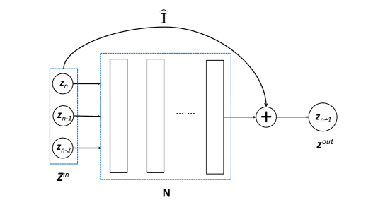
Fig. 1: Illustration of the proposed neural network with $n_{M}=2$ memory steps.

It is straightforward to see that this network creates a mapping

$$\mathbf{z}_{n+1}=\mathbf{z}_{n}+\mathbf{N}(\mathbf{z}_{n},\mathbf{z}_{n-1},\dots,\mathbf{z}_{n-n_{M}};\Theta),\qquad n\geq n_{M}.$$ (17)

3.4 Data, Network Training and Prediction

To train the network (16), we re-organize the data set (2). Let $T_{M}$ be the memory length. With time step $\Delta$ chosen, we have $n_{M}=\lfloor T_{M}/\Delta\rfloor$.

For the trajectory data (2) on $\mathbf{z}$, let us consider each of the $i$-th trajectory data, where $i=1,\dots,N_{T}$. We assume $K^{(i)}\geq n_{M}+2$. That is, each trajectory needs to contain at least $(n_{M}+2)$ data entries. (Otherwise this trajectory is discarded.) We then select a sequence of $(n_{M}+2)$ data entries of consecutive time instances along this trajectory and group them into two vectors, with the first one as the concatenation of the first $(n_{M}+1)$ entries in the form of (14) and the second one as the last entry, in the following form,

$$\left\{\mathbf{Z}^{(i)}_{j},\mathbf{z}^{(i)}_{j}\right\},\qquad j=1,\dots,J^{(i)},\quad$$ (18)

where $J^{(i)}$ is the number of such selected sequences of length $(n_{M}+2)$, and

$$\begin{split}\mathbf{Z}^{(i)}_{j}&=\left[\mathbf{z}\left(t^{(i)}_{k_{j}}\right)^{\top},\dots,\mathbf{z}\left(t^{(i)}_{k_{j}+n_{M}}\right)^{\top},\mathbf{z}\left(t^{(i)}_{k_{j}+n_{M}+1}\right)^{\top}\right]^{\top}\in\mathbb{R}^{D},\\ \mathbf{z}^{(i)}_{j}&=\mathbf{z}\left(t^{(i)}_{k_{j}+n_{M}+2}\right)\in\mathbb{R}^{d}.\end{split}$$ (19)

Here $k_{j}$ is the “starting” position of this sequence in the $i$-th trajectory. Obviously, when the total number of data entries along the trajectory is exactly $(n_{M}+2)$, the starting position has to be $k_{j}=1$ and the number of such groupings is $J^{(i)}=1$.

When the number of data entries is more than $(n_{M}+2)$, one may choose $J^{(i)}>1$ number of such groups. We here discuss two straightforward selections.

• Deterministic selection. This is done by selecting the starting position sequentially from $k_{j}=1$ to $k_{j}=K^{(i)}-n_{M}-1$, and then for each selected starting position take a sequence of $(n_{M}+2)$ to form the group (18). This results in $J^{(i)}=K^{(i)}-n_{M}-1$ number of groups.

• Random selection. Choose $J^{(i)}<K^{(i)}-n_{M}-1$ as the number of selected groups. Randomly selected $J^{(i)}$ starting position from the index set $\{1,\cdots,K^{(i)}-n_{M}-1\}$. And for each selected starting position, form a group in the form of (18).

In our numerical studies, we have found the random selection to be more effective than the deterministic selection.

The aforementioned group selection procedure is then repeated for each $i=1,\dots,N_{T}$, trajectory. We then form the training data set by collecting all the groups from (18)

$$\mathcal{Z}=\left\{\mathbf{Z}_{j},\mathbf{z}_{j}\right\},\qquad j=1,\dots,J,\quad$$ (20)

where $J=J^{(1)}+\cdots+J^{(N_{T})}$ is the total number of data groupings. This is the training data set, where we have re-labeled the entries using a single index $j$ for computational convenience.

By using the data set (20) and our network structure (16), we then train the neural network by finding its parameter set $\Theta^{*}$ that minimizes the mean-squared loss, i.e.,

$$\Theta^{*}=\operatornamewithlimits{argmin}_{\Theta}\frac{1}{J}\sum_{j=1}^{J}\left\|\mathbf{z}^{out}_{j}(\Theta)-\mathbf{z}_{j}\right\|^{2},$$ (21)

where

$$\mathbf{z}^{out}_{j}(\Theta)=\left[\widehat{\mathbf{I}}+{\mathbf{N}}(\cdot,\Theta)\right]\left(\mathbf{Z}_{j}\right),\qquad j=1,\dots,J,$$

is the network output via (16) for input $\mathbf{Z}_{j}$. Upon finding the optimal network parameter $\Theta^{*}$, we obtain a trained network model

$$\mathbf{z}^{out}=\left[\widehat{\mathbf{I}}+{\mathbf{N}}(\cdot,\Theta^{*})\right]\left(\mathbf{Z}^{in}\right).$$ (22)

This in turn defines a predictive model for the unknown dynamical system for the observed variables $\mathbf{z}$,

$$\left\{\begin{split}&\mathbf{z}_{n+1}=\mathbf{z}_{n}+\mathbf{N}(\mathbf{z}_{n},\mathbf{z}_{n-1},\dots,\mathbf{z}_{n-n_{M}};\Theta^{*}),\qquad n\geq n_{M},\\ &\mathbf{z}_{n}=\mathbf{z}(t_{n}),\qquad n=0,\dots,n_{M}-1.\end{split}\right.$$ (23)

With $n_{M}$ initial data on $\mathbf{z}$, one can iteratively apply the network model to predict the evolution of $\mathbf{z}$ at later time.

It is worthwhile to discuss the difference between the trained network model (23) and Euler forward approximation of the d-AMZ equation (12). If the operators $\mathbf{R}$ and $\mathbf{M}$ in (12) are known, its Euler forward approximation takes the following form,

$$\left\{\begin{split}&\widetilde{\mathbf{z}}_{n+1}=\widetilde{\mathbf{z}}_{n}+\Delta\left[\mathbf{R}(\widetilde{\mathbf{z}}_{n})+\mathbf{M}(\widetilde{\mathbf{z}}_{n},\widetilde{\mathbf{z}}_{n-1},\dots,\widetilde{\mathbf{z}}_{n-n_{M}})\right],\qquad n\geq n_{M},\\ &\widetilde{\mathbf{z}}_{n}=\mathbf{z}(t_{n}),\qquad n=0,\dots,n_{M}.\end{split}\right.$$ (24)

This obviously induces temporal discretization error. In this case of Euler forward the error is $O(\Delta)$.

Although our model (23) and the Euler approximation (24) resemble each other, we emphasize that they are fundamentally different. Our neural network model (23) is a direct nonlinear approximation to the time average of the right-hand-side of (12), whereas the Euler method (24) is a pre-selected piecewise constant approximation to the time average. Therefore, the Euler method requires the knowledge of the operators $\mathbf{R}$ and $\mathbf{M}$, which is not available in our setting, and has $O(\Delta)$ temporal error. Our neural network model (23), on the other hand, does not contain this temporal error and uses data to directly approximate the operators in (12). For autonomous dynamical systems, it was shown that the neural network model is exact in temporal integration ([17]), with the only source of errors being the training error (21). Error analysis for the reduced system model (23) in this paper is considerably more complicated, and will be pursued in separate studies.

4 Numerical Examples

In this section, we present numerical examples to examine the performance of the proposed learning method. Our examples include two linear systems, where the exact Mori-Zwanzig formulation for the reduced system is available, and two nonlinear systems, one of which is chaotic. Since in all examples the true models are available, we are able to compute their solutions with high resolution numerical solver. This creates reference solutions, with which we compare the predictive results by our neural network models. For the chaotic system, an analytically defined reduced model is also available, and its results are used to compare against those of our trained reduced network model.

The training data for the reduced variables are synthetic and generated by solving the true systems with high resolution. In each example, we first choose a range of interest for the full variables $\mathbf{x}=(\mathbf{z};\mathbf{w})\in D_{\mathbf{x}}$. This will be the range in which we seek an accurate model for the observed variable $\mathbf{z}\in D_{\mathbf{z}}\subset D_{\mathbf{x}}$. We then randomly generate $N_{T}$ number of initial conditions using the uniform distribution on $D_{\mathbf{x}}$. For each $i=1,\dots,N_{T}$, we solve the underlying true system of equations with high resolution and march forward in time with time step $\Delta$. In all examples, we set $\Delta=0.02$. Each trajectory is marched forward in time for $K^{(i)}=K=\mathop{\operator@font const}\nolimits$ steps. We then only keep the trajectory data for the observed variables $\mathbf{z}$ to create our raw data set (2). For benchmarking purpose, we did not add additional noises to the data. This allows us to examine more closely the properties of the method.

The memory length $T_{M}$ (9) is problem dependent. In each example, we progressively increase the memory length to achieve converged results. The number of memory steps is then determined as $n_{M}=\lfloor T_{M}/\Delta\rfloor$. We then randomly select $J^{(i)}$ number of sequences of length $(n_{M}+2)$ data entries from each of the $i$-th trajectory data, where $i=1,\dots,N_{T}$, as described in Section 3.4, to form the training data set (20). We fix $J^{(i)}=J_{0}$ to be a constant for all trajectories. The total number of data entries in the training data set (20) is then $J=J_{0}\times N_{T}$. In all the tests, we purposefully keep the number of data $J$ to be roughly $5\sim 10$ times of the number of parameters in the neural network structure. This is to avoid any potential training accuracy loss due to lack of data and/or overfitting, thus allowing us to focus on the properties of the numerical methods. In practical computations when data are limited, proper care needs to be taken during network trianing. This is well recognized and well studied topic outside the scope of this paper.

4.1 Example 1: Small Linear System

We first consider a simple linear system

$$\begin{cases}\dot{x}_{1}=x_{1}-4x_{2},\\ \dot{x}_{2}=4x_{1}-\alpha x_{2},\end{cases}$$ (25)

where $\alpha$ is a parameter controlling the decay rate of the solution. We set $z=x_{1}$ to be the observed variable and $w=x_{2}$ to be the unobserved variable. Note that this is a simplified case of the well documented case

$$\begin{cases}\dot{\mathbf{z}}=\mathbf{A}_{11}\mathbf{z}+\mathbf{A}_{12}\mathbf{w},\\ \dot{\mathbf{w}}=\mathbf{A}_{21}\mathbf{z}+\mathbf{A}_{22}\mathbf{w},\end{cases}$$ (26)

where the matrices $\mathbf{A}$’s are of proper sizes. The exact Mori-Zwanzig dynamics for the observed variable $\mathbf{z}$ is known as

$$\frac{d\mathbf{z}}{dt}=\mathbf{A}_{11}\mathbf{z}+\mathbf{A}_{12}\int_{0}^{t}e^{\mathbf{A}_{22}(t-s)}\mathbf{A}_{21}\mathbf{z}(s)ds+\mathbf{A}_{21}e^{\mathbf{A}_{22}t}\mathbf{w}(0).$$ (27)

In our example, we set the domain of interest to be $D_{\mathbf{x}}=[-2,2]^{2}$. For data generation, we set all trajectory length to be $(n_{M}+2)$. Hence, each trajectory contributes to one data entry ($J_{0}=1)$ in the training data set (20). Based on the solution behavior, two cases are presented here: (1) Fast decay case for $\alpha=2$; and (2) Slow decay case for $\alpha=1.1$.

We first consider the fast decay case. In Fig. 2, we plot the neural network model prediction of the observed variable $x_{1}$ for up to $t=20$, using memory term $n_{M}=30$, which corresponds to memory length $T_{M}=n_{M}\Delta=0.6$. We observe that, for four arbitrarily chosen initial conditions, the network predictions match the exact true solution well. Since the solution decay to zero fast, we did not conduct model prediction over longer term.

Longer-term predictions are conducted for the slow decaying case with $\alpha=1.1$, as shown in Fig. 3. The NN model is constructed using memory lenght $T_{M}=0.6$. The model prediction again shows good agreement with the exact solution for up to $t=100$.

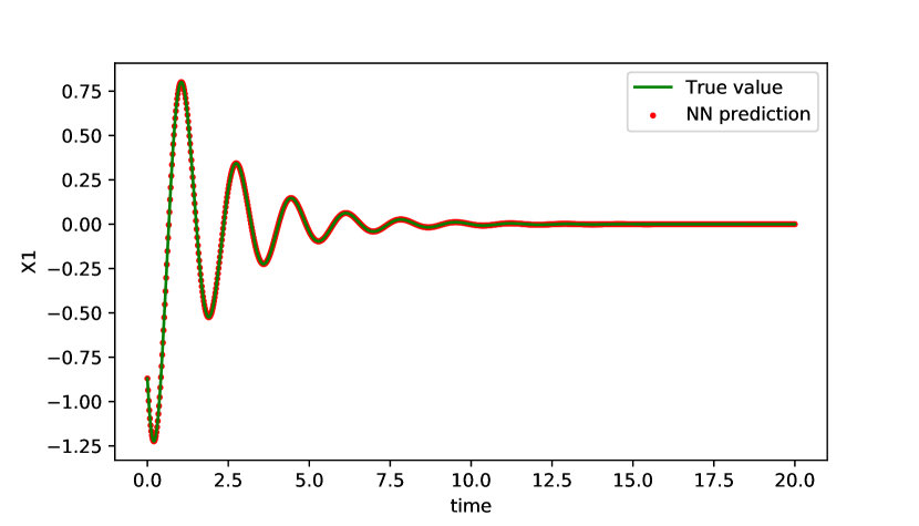
(a) Initial value = $(-0.87,0.65)$.

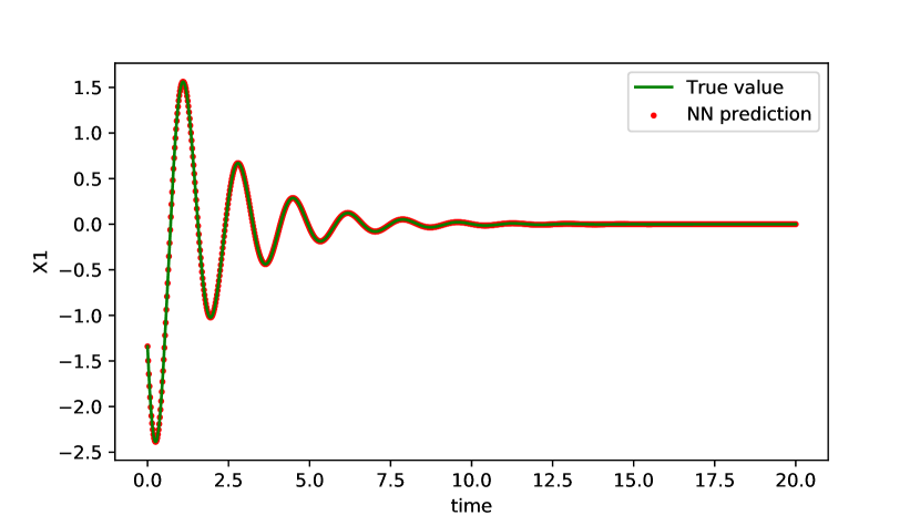
(b) Initial value = $(-1.34,1.7)$.

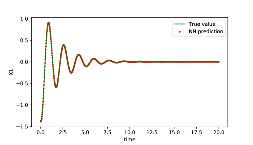
(c) Initial value = $(-1.37,-0.11)$.

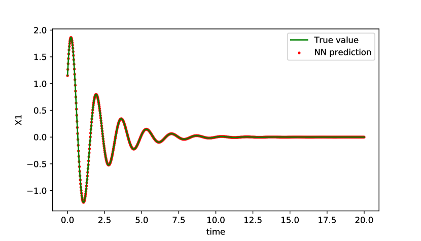
(d) Initial value = $(1.15,-1.21)$.

Fig. 2: Example 1: fast decay case. Neural network model prediction of $x_{1}$ with memory length $T_{M}=0.6$ using four different initial conditions.

(a) Initial value = $(-1.38,-0.11)$.

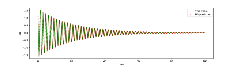
(b) Initial value = $(1.1,1.45)$.

Fig. 3: Example 1: slow decay case. Neural network model prediction of $x_{1}$ with memory length $T_{M}=0.6$ using two different initial conditions.

We then examine the effect of different memory length in the NN modeling. The prediction errors produced by the models with varying $n_{M}$ are shown in Fig. 4. We observe that the NN models become more accurate as the memory length increases. The accuracy starts to saturate around $n_{M}=30$, which corresponds to memeory length $T_{M}=0.6$. Further increasing the memory length induces no further accuracy improvement.

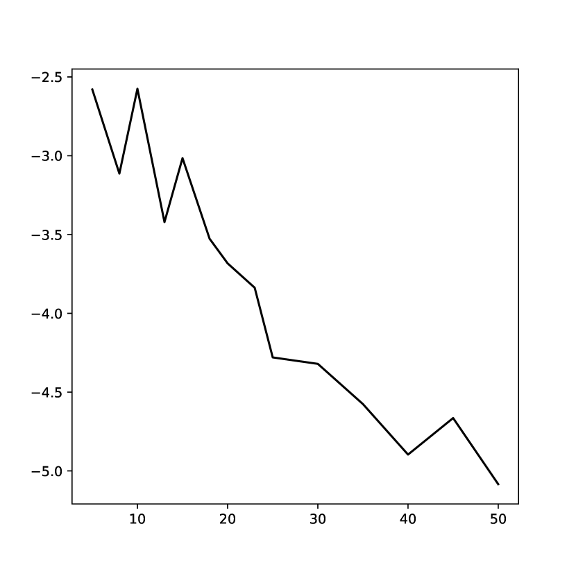
(a) Fast decay case.

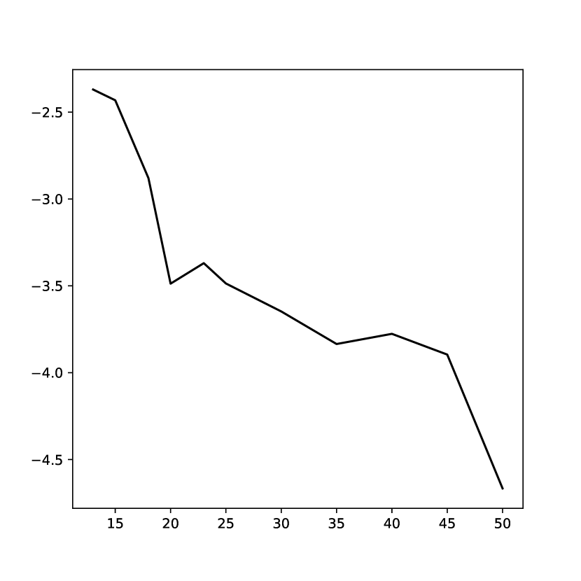
(b) Slow decay case.

Fig. 4: Example 1: NN prediction errors in $\log$ scale vs. number of memory terms.

4.2 Example 2: Nonlinear System

We now consider a damped pendulum system, which is a simple nonlinear system.

$$\begin{cases}\dot{x}_{1}=x_{2},\\ \dot{x}_{2}=-\alpha x_{2}-\beta\sin x_{1},\end{cases}$$ (28)

where $\alpha=0.1$ and $\beta=8.91$. The domain of interest is set as $D_{\mathbf{x}}=[-2,2]\times[-4,4]$. The observed variable is $z=x_{1}$ and we seek to construct an NN model for its prediction. Our training data sets (20) are generated by collecting $J_{0}=5$ sequences of $x_{1}$ data randomly from each $x_{1}$ trajectory data of length $K=50$. The memory step is tested for $n_{M}=3,5,8,10,13,15,18,20$. The numerical errors in the model predictions with different memory steps are shown in Fig. 5. We observe that the accuracy improvement over increasing $n_{M}$ starts to saturate with $n_{M}\geq 10$. The NN model predictive result with $n_{M}=20$ is shown in Fig. 6. This corresponds to memory length $T_{M}=n_{M}\times\Delta=0.4$. We again observe very good agreement with the reference solution for long-term integration up to $t=100$.

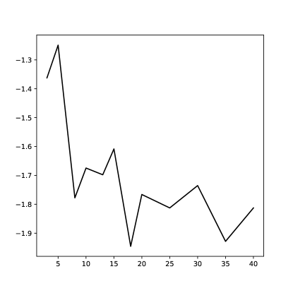
Fig. 5: Example 2. Prediction errors in $\log$ scale vs. the number of memory steps.

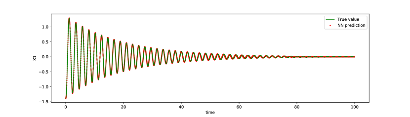
(a) Initial value = $(-1.38,-0.22)$.

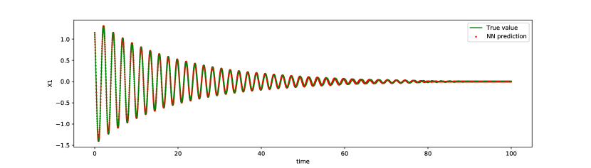
(b) Initial value = $(1.15,-2.43)$.

Fig. 6: Example 2. NN model prediction of $x_{1}$ with memory length $T_{M}=0.4$ using two arbitrary initial conditions.

4.3 Example 3: Chaotic System

We now consider a nonlinear chaotic system ([14])

$$\begin{cases}\dot{x}_{1}=-x_{2}-x_{3},\\ \dot{x}_{2}=x_{1}+\frac{1}{5}x_{2},\\ \dot{x}_{3}=\frac{1}{5}+y-5x_{3},\\ \dot{y}=-\frac{y}{\epsilon}+\frac{x_{1}x_{2}}{\epsilon},\end{cases}$$ (29)

where $\epsilon>0$ is a small parameter. In this example, we choose the observed variables to be $\mathbf{z}=(x_{1},x_{2},x_{3})^{\top}$ and let the fast variable $y$ be the unobserved variable. Note that for this system, there exists a homogenized system for the slow variables $(x_{1},x_{2},x_{3})$,

$$\begin{cases}\dot{x}_{1}=-x_{2}-x_{3},\\ \dot{x}_{2}=x_{1}+\frac{1}{5}x_{2},\\ \dot{x}_{3}=\frac{1}{5}+x_{3}(x_{1}-5).\end{cases}$$ (30)

The reduced system is a good approximation for the true system when $\epsilon\ll 1$. Here we will construct NN models for the reduced variables $\mathbf{z}$ and compare the prediction results against the true solution of (29), as well as those obtained by the reduced system (30). We set $\epsilon=0.01$, in which case the reduced system (30) is considered an accurate approximation of the true system.

The domain of interest is set to be $D_{\mathbf{x}}=[-7.5,10]\times[-10,7.5]\times[0,18]\times[-1,100]$, which is sufficiently large to enclose the solution trajectories for different initial conditions. To generate training data set (20), we solve the true system (29) using randomly sampled initial conditions via a high resolution numerical solver and record the trajectories of $\mathbf{z}$ with length $K=100$, which corresponds to a time lapse of $K\Delta=2$. In each trajectory, we randomly select $J_{0}=5$ sequences of data with length $(n_{M}+2)$ for our training data set. Different memory steps of $n_{M}=10,20,30,40,50,60,70,80$ are examined. This corresponds to memory length $T$ ranging from 0.2 to 1.6. Our results indicate that $n_{M}=60$, i.e, $T_{M}=1.2$, delivers accurate predictions. Further increasing memory length does not lead to better predictions.

The evolution of prediction errors, measured in $\ell_{2}$-norm against the reference true solution, are shown in Fig. 7, for both our neural network model and the reduced model (30) for long term prediction up to $t=400$. Here the errors are averaged over 100 simulations using randomly selected initial conditions. We observe that our NN model produces noticebaly more accurate results than the reduced system (30), even for the case of small $\epsilon$ when (30) is supposed to be highly accurate. More importantly, the NN model exhibits much smaller error growth over long time, compared to the reduced system (30). The solution behavior is shown in Fig. 8, for long-term integration up to $t=400$ for the first component $x_{1}$. (Behavior for other components are similar.) The NN model produces visually better results than the reduced system (30), when compared to the true solution, especially in term of capturing the phase/frequency of the solution.

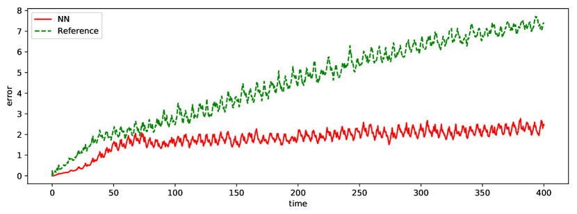
Fig. 7: Example 3. Errors in model predictions over time, by the NN model with $T_{M}=1.2$ and the reduced system (30). The errors are averaged over 100 simulations of different initial conditions.

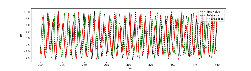
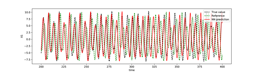
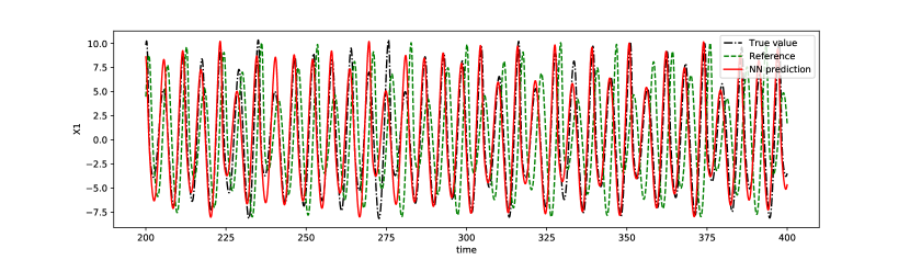
Fig. 8: Example 3. Long-term model prediction of $x_{1}$ by the NN model with $T_{M}=1.2$ and the reduced system (30). Zoomed view for $t\in[200,400]$ with three aribitrarily chosen initial conditions.

4.4 Example 4: Larger Linear System

We now consider a larger linear system involving 20 state variables $\mathbf{x}=(\mathbf{p};\mathbf{q})\in\mathbb{R}^{20}$,

$$\begin{cases}\dot{\mathbf{p}}=\Sigma_{11}\mathbf{p}+(\mathbf{I}+\Sigma_{12})\mathbf{q},\\ \dot{\mathbf{q}}=-(\mathbf{I}+\Sigma_{21})\mathbf{p}-\Sigma_{22}\mathbf{q},\end{cases}$$ (31)

where $\mathbf{p},\mathbf{q}\in\mathbb{R}^{10}$, $\mathbf{I}$ is identity matrix of size $10\times 10$, and $\Sigma_{ij}\in\mathbb{R}^{10\times 10}$, $i=1,2,j=1,2$. We set the observed variables to be $\mathbf{z}=\mathbf{p}\in\mathbb{R}^{10}$ and let $\mathbf{w}=\mathbf{q}\in\mathbb{R}^{10}$ be the unobserved variables. Note that as a linear system (26), the exact Mori-Zwanzig equations for the reduced variables $\mathbf{z}$ are available in analytical form (27). We set the entries of $\Sigma_{ij}$ to be small and consider them as perturbations to an oscillatory system. The exact values of the entries of matrices $\Sigma_{ij}$ are presented in Appendix, for self completeness of the paper.

The domain of interest is set to be $D_{\mathbf{x}}=[-2,2]^{20}$. In generating the training data sets, we randomly select $J_{0}=5$ sequences of data from each trajectory of $\mathbf{z}$ with length $K=100$. We test different memory steps for $n_{M}=10,15,20,25,30,35,40,45,50$. Our experiments show that $n_{M}=30$, which corresponds to a memory length $T_{M}=0.6$, provides accurate prediction. Further increasing memory length does not lead to better prediction accuracy. Our NN model predictions for long-term integration up to $t=150$ are shown in Fig. 9. Compared to the reference solution obtained from the true system, we observe very good agreement, where the NN predictions overlap the true solutions to be visually indistinguishable.

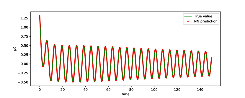
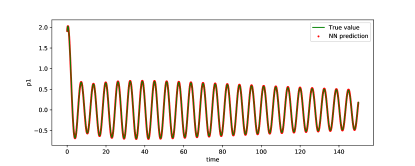
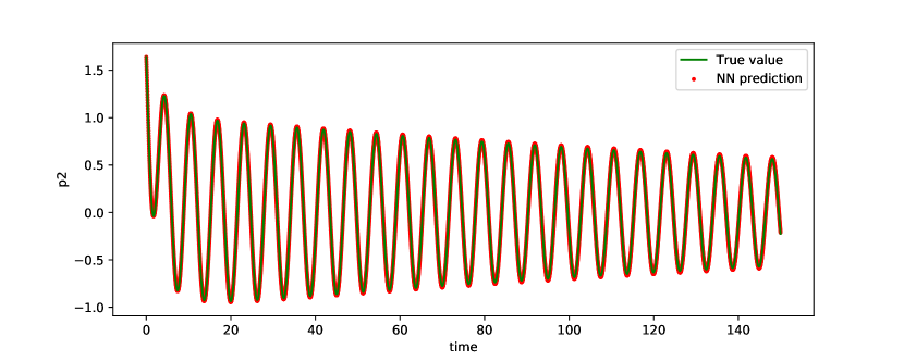
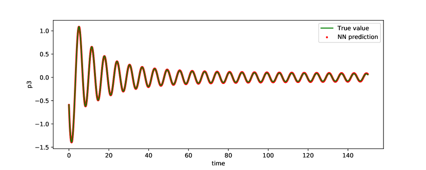
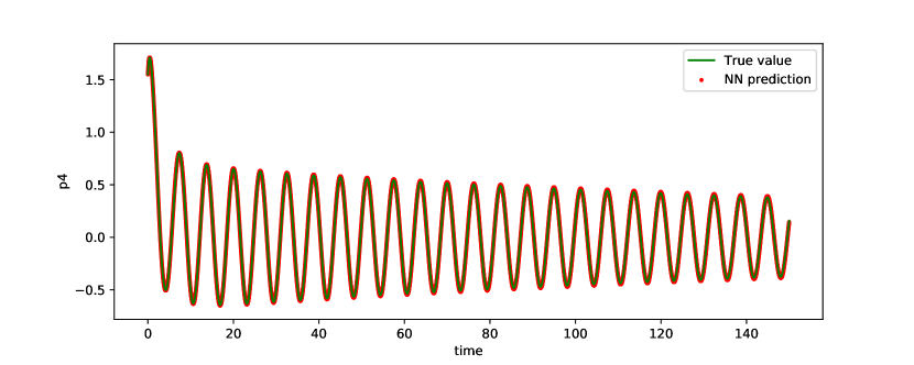
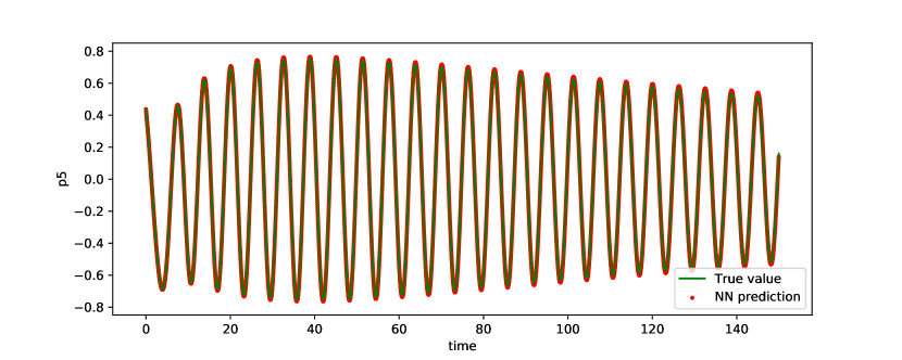
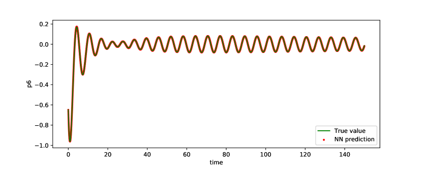
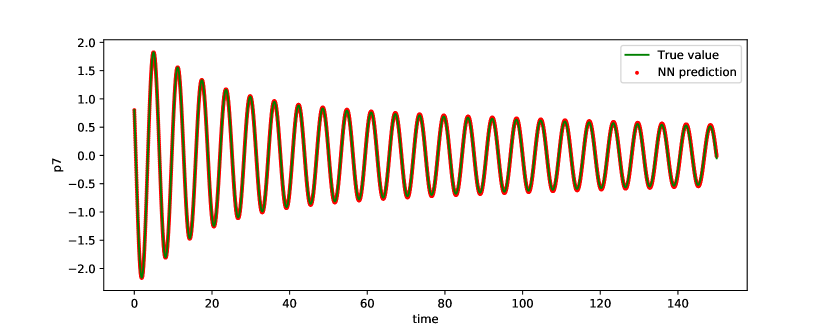
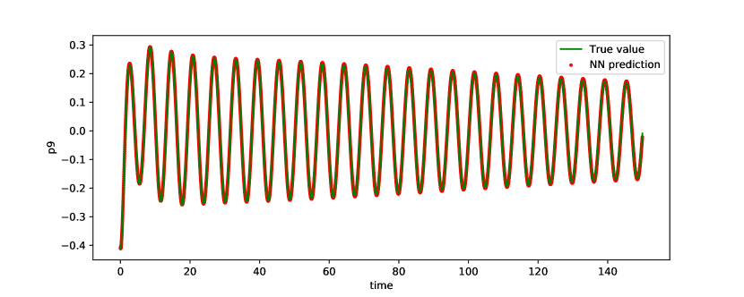
Fig. 9: Example 4. NN model prediction of $\mathbf{p}$ for up to $t=150$, with memory length $T_{M}=0.6$.

5 Conclusion

We present construction of deep neural network (DNN) model to approximating unknown dynamical systems when only a subset of variables are observed. The DNN model then provides a reduced model for the unknown dynamical system. Based on Mori-Zwanzig (MZ) formulation for reduced systems, we established a discrete Mori-Zwanzig formulation with finite memory assumption. We then designed a straightforward DNN structure to explicitly incorporate the system memory into the predictive model. Numerical tests on both linear and nonlinear systems demonstrated good accuracy of the DNN models. This invites further in-depth study of the approach, both theoretically and numerically.

Appendix A Details of Example 4 in Section 4.4

The detailed setting of Example 4 is

$$\begin{cases}\dot{\mathbf{p}}=\Sigma_{11}\mathbf{p}+(\mathbf{I}+\Sigma_{12})\mathbf{q},\\ \dot{\mathbf{q}}=-(\mathbf{I}+\Sigma_{21})\mathbf{p}-\Sigma_{22}\mathbf{q},\end{cases}$$ (32)

where $\mathbf{p},\mathbf{q}\in\mathbb{R}^{10}$, $\mathbf{I}$ is identity matrix of size $10\times 10$, and $\Sigma_{ij}\in\mathbb{R}^{10\times 10}$, $i=1,2,j=1,2$. The matices $\Sigma_{ij}$ are defined as follows.

$$\Sigma_{11}\times 10^{3}=$$

$$\left(\begin{array}[]{rrrrrrrrrr}-6.09&5.79&-0.945&-12.1&9.38&-12.4&4.92&3.71&1.17&4.73\\ -9.57&-8.88&-12.1&-12.9&5.11&26.5&-7.33&-8.01&-21.6&-10.2\\ -0.733&6.2&10.7&-6.06&-7.07&-1.7&-16.4&6.69&-1.59&7.69\\ 7.83&12.5&5.77&-14.9&-17.8&-1.01&-4.05&-15&-6.61&-4.94\\ 8.1&4.13&4.21&23.3&-4.63&1.77&-14.9&17.9&-17.1&-8.19\\ -7.68&6.98&27.6&19&20.9&12.2&15.6&-11.2&-3.56&-2.47\\ -14.9&-5.73&-19.7&-8.77&-9.17&-2.95&-9.48&-2.95&5.43&15.4\\ -1.84&2.05&-1.98&3.83&-4.06&7.72&4.04&-13.7&20.3&0.509\\ 12.1&19.7&-14.3&12.6&-4.67&9.72&5.87&0.664&-10.8&-18.2\\ 3.07&3.65&3.88&7.44&12.7&13.5&-6.66&-23.9&-11.7&16.6\end{array}\right),$$

$$\Sigma_{12}\times 10^{3}=$$

$$\left(\begin{array}[]{rrrrrrrrrr}11.7&-12.3&-8.87&-6.86&-9.6&11&25.6&-0.155&17.8&-10.9\\ 12.9&3.28&2.84&3.35&16.6&5.96&6.99&-20.2&8.37&-8.87\\ -0.154&-16.5&12.1&0.381&11.2&-2.59&12.8&3.32&-10.9&-3.81\\ 6.49&15.8&-0.273&9.05&-3.15&0.976&-7.35&0.889&6.41&15.6\\ 4.86&-1.52&0.118&17.8&-5.08&-4.96&-2.89&3&22.4&16.4\\ 7.83&-9.66&-2.09&5.97&3.97&19.2&4.03&-15.3&-8.5&-15.8\\ -4.61&-4.98&17&-14&-17.5&0.104&-27.5&10.9&-17.9&-5.9\\ 3.88&14&-2.63&-7.27&-21&-0.403&-2.18&-22&2.01&-2.45\\ 14.4&-4.65&-8.67&-23.2&-2.73&9.58&-13.9&0.415&10.3&17.5\\ -16.8&8.18&-12.3&14.2&-18.4&-10.2&-11.4&-1.99&-2.65&-2.34\end{array}\right),$$

$$\Sigma_{21}\times 10^{3}=$$

$$\left(\begin{array}[]{rrrrrrrrrr}-3.51&-4.91&-4.51&-15.8&-12&-5.72&-9.52&-14.3&0.745&-11.8\\ 1.8&2.07&8.78&5.3&-5.25&5.7&0.0957&9.77&2.17&12.8\\ -9.87&5.19&0.884&2.59&-7.95&5.56&6.41&16.4&15.6&14.3\\ 10.4&7.14&15.5&-6.6&5.33&-3.37&2.8&-9.61&8&-16.8\\ 15.5&19.6&-1.1&0.6&8.38&7.62&3.43&1.28&10.3&-4.76\\ 0.119&-9.43&-6.6&-9.99&-10.5&17.8&13.5&-6.63&-0.566&-1.81\\ -6.77&-1.42&7.46&3.32&11.7&1.3&-6.21&6.9&3.89&18.9\\ 2.93&15.1&-4.65&11.1&9.13&-9.58&-7.04&6.88&-4.07&10.2\\ -6.02&14&-5.91&-4.92&0.851&0.652&-2.57&0.835&-5.14&10.6\\ 1.41&5.8&-2.31&6.17&13.3&3.57&15.9&-0.753&-0.818&-10.3\end{array}\right),$$

$$\Sigma_{22}\times 10^{3}=$$

$$\left(\begin{array}[]{rrrrrrrrrr}1500&124&814&-104&-179&-223&-731&-189&-400&242\\ 124&836&679&277&197&-515&-52.1&-273&101&301\\ 814&679&1500&651&755&-605&-379&-546&-225&223\\ -104&277&651&1960&720&-782&-299&-775&-180&506\\ -179&197&755&720&2290&-973&518&-19.1&-604&-369\\ -223&-515&-605&-782&-973&1290&-400&412&314&-420\\ -731&-52.1&-379&-299&518&-400&1960&68.3&455&-316\\ -189&-273&-546&-775&-19.1&412&68.3&576&-53.6&-332\\ -400&101&-225&-180&-604&314&455&-53.6&1030&265\\ 242&301&223&506&-369&-420&-316&-332&265&1090\end{array}\right).$$

References

- [1] D. Bernstein, Optimal prediction of Burgers’s equation, Multiscale Model. Simul., 6 (2007), p. 27–52.
- [2] C. Brennan and D. Venturi, Data-driven closures for stochastic dynamical systems, J. Comput. Phys., 372 (2018), p. 281–298.
- [3] S. L. Brunton, J. L. Proctor, and J. N. Kutz, Discovering governing equations from data by sparse identification of nonlinear dynamical systems, Proc. Natl. Acad. Sci., 113 (2016), pp. 3932–3937.
- [4] Z. Chen and D. Xiu, On generalized residue network for deep learning of unknown dynamical systems, J. Comput. Phys., submitted (2020).
- [5] A. Chertock, D. Gottlieb, and A. Solomonoff, Modified optimal prediction and its application to a particle-method problem, J. Sci. Comput., 37 (2008), pp. 189–201.
- [6] A. J. Chorin, O. H. Hald, and R. Kupferman, Optimal prediction with memory, Physica D: Nonlinear Phenomena, 166 (2002), pp. 239–257.
- [7] O. Hald and P. Stinis, Optimal prediction and the rate of decay for solutions of the Euler equations in two and three dimensions, Proc. Natl. Acad. Sci., 104 (2007), p. 6527–6532.
- [8] K. He, X. Zhang, S. Ren, and J. Sun, Deep residual learning for image recognition, in Proceedings of the IEEE conference on computer vision and pattern recognition, 2016, pp. 770–778.
- [9] S. H. Kang, W. Liao, and Y. Liu, IDENT: Identifying differential equations with numerical time evolution, arXiv preprint arXiv:1904.03538, (2019).
- [10] H. Lei, N. Baker, and X. Li, Data-driven parameterization of the generalized Langevin equation, Proc. Natl. Acad. Sci., 113 (2016), p. 14183–14188.
- [11] Z. Long, Y. Lu, and B. Dong, PDE-Net 2.0: Learning PDEs from data with a numeric-symbolic hybrid deep network, arXiv preprint arXiv:1812.04426, (2018).
- [12] Z. Long, Y. Lu, X. Ma, and B. Dong, PDE-net: Learning PDEs from data, in Proceedings of the 35th International Conference on Machine Learning, J. Dy and A. Krause, eds., vol. 80 of Proceedings of Machine Learning Research, Stockholmsmässan, Stockholm Sweden, 10–15 Jul 2018, PMLR, pp. 3208–3216.
- [13] H. Mori, Transport, collective motion, and brownian motion, Progress of theoretical physics, 33 (1965), pp. 423–455.
- [14] G. Pavliotis and A. Stuart, Multiscale methods: averaging and homogenization, Springer, 2008.
- [15] T. Qin, Z. Chen, J. Jakeman, and D. Xiu, A neural network approach for uncertainty quantification for time-dependent problems with random parameters, Inter. J. Uncertainty Quantification, submitted (2020).
- [16] T. Qin, K. Wu, and D. Xiu, Data driven governing equations approximation using deep neural networks, J. Comput. Phys., 395 (2019), pp. 620 – 635.
- [17] T. Qin, K. Wu, and D. Xiu, Structure-preserving method for reconstructing unknown Hamiltonian systems from trajectory data, SIAM J. Sci. Comput., submitted (2019).
- [18] M. Raissi, Deep hidden physics models: Deep learning of nonlinear partial differential equations, Journal of Machine Learning Research, 19 (2018), pp. 1–24.
- [19] M. Raissi, P. Perdikaris, and G. E. Karniadakis, Physics informed deep learning (part i): Data-driven solutions of nonlinear partial differential equations, arXiv preprint arXiv:1711.10561, (2017).
- [20] M. Raissi, P. Perdikaris, and G. E. Karniadakis, Physics informed deep learning (part ii): Data-driven discovery of nonlinear partial differential equations, arXiv preprint arXiv:1711.10566, (2017).
- [21] M. Raissi, P. Perdikaris, and G. E. Karniadakis, Multistep neural networks for data-driven discovery of nonlinear dynamical systems, arXiv preprint arXiv:1801.01236, (2018).
- [22] S. H. Rudy, S. L. Brunton, J. L. Proctor, and J. N. Kutz, Data-driven discovery of partial differential equations, Science Advances, 3 (2017), p. e1602614.
- [23] S. H. Rudy, J. N. Kutz, and S. L. Brunton, Deep learning of dynamics and signal-noise decomposition with time-stepping constraints, J. Comput. Phys., 396 (2019), pp. 483–506.
- [24] H. Schaeffer, Learning partial differential equations via data discovery and sparse optimization, Proceedings of the Royal Society of London A: Mathematical, Physical and Engineering Sciences, 473 (2017).
- [25] H. Schaeffer and S. G. McCalla, Sparse model selection via integral terms, Phys. Rev. E, 96 (2017), p. 023302.
- [26] H. Schaeffer, G. Tran, and R. Ward, Extracting sparse high-dimensional dynamics from limited data, SIAM Journal on Applied Mathematics, 78 (2018), pp. 3279–3295.
- [27] P. Stinis, Higher order Mori–Zwanzig models for the Euler equations, Multiscale Model. Simul., 6 (2007), p. 741–760.
- [28] Y. Sun, L. Zhang, and H. Schaeffer, NeuPDE: Neural network based ordinary and partial differential equations for modeling time-dependent data, arXiv preprint arXiv:1908.03190, (2019).
- [29] R. Tibshirani, Regression shrinkage and selection via the lasso, Journal of the Royal Statistical Society. Series B (Methodological), (1996), pp. 267–288.
- [30] G. Tran and R. Ward, Exact recovery of chaotic systems from highly corrupted data, Multiscale Model. Simul., 15 (2017), pp. 1108–1129.
- [31] D. Venturi and G. Karniadakis, Convolutionless Nakajima-Zwanzig equations for stochastic analysis in nonlinear dynamical systems, Proc. R. Soc. A, 470 (2014), p. 20130754.
- [32] Q. Wang, N. Ripamonti, and J. Hesthaven, Recurrent neural network closure of parametric POD-Galerkin reduced-order models based on the Mori-Zwanzig formalism, J. Comput. Phys., https://doi.org/10.1016/j.jcp.2020.109402 (2020).
- [33] K. Wu, T. Qin, and D. Xiu, Structure-preserving method for reconstructing unknown hamiltonian systems from trajectory data, arXiv preprint arXiv:1905.10396, (2019).
- [34] K. Wu and D. Xiu, Numerical aspects for approximating governing equations using data, J. Comput. Phys., 384 (2019), pp. 200–221.
- [35] K. Wu and D. Xiu, Data-driven deep learning of partial differential equations in modal space, J. Comput. Phys., 408 (2020), p. 109307.
- [36] Y. Zhu and D. Venturi, Faber approximation of the Mori-Zwanzig equation, J. Comput. Phys., 372 (2018), pp. 694–718.
- [37] R. Zwanzig, Nonlinear generalized langevin equations, Journal of Statistical Physics, 9 (1973), pp. 215–220.