Sustainability Analysis of Interconnected Food Production Systems via Theory of Barriers

Abstract

Controlled environment agriculture (CEA) is used for efficient food production. Efficiency can be increased further by interconnecting different CEA systems (e.g. plants and insect larvae or fish and larvae), using products and by-products of one system in the other.

These interconnected systems define an overall system that can be described by models of interacting species. It is necessary to identify system parameters (e.g. initial species concentration, harvest rate, feed quality, etc.) such that the resources are not exhausted. For such systems with interacting species, modelled by the Lotka-Volterra equations, a set-based approach based on the recent results of the theory of barriers to exactly determine the so-called admissible set (also known as viability kernel) and the maximal robust positively invariant set is presented. Using an example of a larvae-fish based production system, steps to obtain special trajectories which are the boundaries of the admissible set are shown. This admissible set is used to prevent the under and over population of the species in the CEA. Furthermore, conditions of the system parameters are stated, such that the existence of these trajectories can be guaranteed.

1 Introduction

In recent years the general interest in sustainable ecosystems has increased, because of environmental changes and publicly well known challenges concerning, for example conservation of biodiversity, overexploitation of marine ecosystems, and exhaustion of fossil resources. It has also been recognised that human interventions yield ecological stresses with irreversible consequences. For instance, the loss of species or destruction of habitat. Therefore, sustainable management of ecological systems becomes more and more important as described in De Lara and Doyen (2008).

Food production industry is one of the biggest contributors to this ecosystem imbalance (Barnosky et al., 2011; Funabashi, 2018). Modern farming techniques such as controlled environment agriculture (CEA), also used in space research, are evaluated to improve the productivity and address the sustainability aspects through the use of different organisms (e.g. plant, fishes, insects) interacting through resource exchange (Conrad et al., 2017). Such studies are new in CEA and can utilize methods and tools developed for conventional farming and ecosystem management.

The Lotka-Volterra equations for describing the species interaction and the viability theory for finding the viability kernel to prevent species exhaustion, are widely used in the marine- and terrestrial ecosystem studies. For example, in Bayen and Rapaport (2019) the viability kernel was found to prevent the extinction of prey, in Eisenack et al. (2006) the viability theory was applied to design management framework for fisheries, and for exhaustible natural resource a viable control approach is presented via viability theory in (Martinet and Doyen, 2007).

The aforementioned species interaction dynamics are also used to address different aspects of agriculture and food production. Development of protocols for food production optimization (Fort et al., 2017), effects of organic management practices in pest control (Schmidt et al., 2014), optimization of harvesting policy (Zhang et al., 2000), design of ecosystems for nitrification in aquaponics system (Graham et al., 2007), and modeling the growth of Hermetia illucens (Gligorescu et al., 2019) are some of the examples applying these interaction dynamics.

In this paper we analyse the admissible set and the maximal robust positively invariant (MRPI) set of the widely studied Lotka-Volterra model, with state and input constraints, on a food production system with species interaction. We use the theory of barriers in constrained nonlinear systems as developed in De Dona and Lévine (2013) and Esterhuizen et al. (2019) to analyse these sets, describing how to construct them, and stating algebraic conditions of the system parameters under which they exist. We use these sets to obtain information pertaining to management strategies for sustainable operation of food production systems. We illustrate our results for a fish and insect-larvae example derived from a combination of aquaculture and insect farming under controlled environments.

The outline of this paper is as follows. In Section 2 a brief overview of the model and its relationship with controlled environment agriculture is established. In Section 3 we briefly cover the theory of barriers. Sections 4 contains the main result of this paper with the analysis of the admissible and positively invariant set for the Lotka-Volterra equations. Section 5 presents a numerical examples and in Section 6 we discuss our analysis. We conclude the paper in Section 7 with a summary and ideas for future research.

2 Idea of sustainable interconnected controlled environment agriculture

In an interconnected CEA system producing different biomass (plant, fish, insect larvae) interaction between the connected systems is established through the exchange of products and by-products (e.g. plant waste as feed for larvae, larvae as feed for fish, fish waste as nutrients for plant). In case of a single CEA system the interconnection can be represented by the species interacting with a food source (e.g. larvae feeding on larvae feed, plant consuming nutrients etc.)

Dynamics of such interactions between the species or between species and resources can be modelled using the Lotka-Volterra equations given by:

$$\begin{split}\dot{x}_{1}&=\alpha x_{1}-\beta x_{1}x_{2}+u_{1}x_{1},\\ \dot{x}_{2}&=\delta x_{1}x_{2}-\gamma x_{2}+u_{2}x_{2},\end{split}$$ (1)

where $x_{1}\in\mathbb{R}_{\geq 0}$ denotes the number of prey (e.g. plant, larvae) and $x_{2}\in\mathbb{R}_{\geq 0}$ denotes the number of predators (e.g. larvae, fish). The parameters $\alpha,\beta,\gamma$ and $\delta$ are positive constants. As per Getz (2012), the best applicable interpretation of the parameters of the Lotka-Volterra equations for biomass production are: $\alpha$, the intrinsic growth rate of the resource (prey); $\beta$, the extraction rate per unit resource per unit consumer (predator); $\delta=\eta\beta$, where $\eta$ is the biomass conversion parameter; and $\gamma$, the intrinsic rate of decline of the consumer in the absence of resource. Furthermore, $u_{i}(t)\in[u_{i}^{\min},u_{i}^{\max}]\subset\mathbb{R}$ for all $t$, with $u_{i}^{\min}\leq u_{i}^{\max}$ $i=1,2$, are constrained inputs that model the intervention into the predator-prey system. In our framework of a CEA system the input is either the introduction of prey or the removal (harvest) of predators. Additionally we have to introduce the limits for the number of prey and predators. The lower limit is naturally given by zero, whereas for the goal of preventing extinction of a species, this number has to be positive. We also introduce an upper limit, since, we act in a controlled environment with a given limit of the habitat for the species, thus, we also want to prevent overpopulation (overproduction). Therefore we need to consider the following constraints $x_{1}(t)\in[\underline{x}_{1},\overline{x}_{1}]\;\forall t$, $0\leq\underline{x}_{1}<\overline{x}_{1}$, $x_{2}(t)\in[\underline{x}_{2},\overline{x}_{2}]\;\forall t$, $0\leq\underline{x}_{2}<\overline{x}_{2}$. These constraints describe the limits for the under- and overpopulation.

As mentioned in the introduction, viability theory plays a decisive role for sustainable strategies related to different ecosystems. In particular, the identification of the viability kernel for predator-prey systems yields information to deduce harvesting strategies which prevent the extinction of a species. In detail, this set describes the population number of predators and prey such that there exists at least one intervention strategy that results in the population remaining within the defined limits. On the boundary of the admissible set there exist exactly one intervention strategy that prevents under- or over-population. The MRPI is interpretable as the population of predators and prey for which every intervention is sustainable. In other word, there does not exist the possibility of crossing the limits for overpopulation or underpopulation. In contrast to the MRPI, every population number outside of the admissible set will lead to a violation of the constraints and therefore to an inevitable overpopulation or underpopulation.

3 Summary of the Theory of Barriers

This section presents a succinct review of the theory of barriers as presented in De Dona and Lévine (2013) and Esterhuizen et al. (2019).

The considered nonlinear system subjected to state and input constraints is defined as follows:

$$\dot{x}(t) =f(x(t),u(t)),\quad x(t_{0})=x_{0},\quad u\in\mathcal{U},$$ (2)

$$g_{i}(x(t)) \leq 0,\forall t\in[t_{0},\infty[,\,\,i=1,2,\dots,p,$$ (3)

where $x(t)\in\mathbb{R}^{n}$ denotes the state; $x_{0}$ is the initial condition at the initial time, $t_{0}$; $u(t)\in\mathbb{R}^{m}$ denotes the input, and $\mathcal{U}$ is the set of all Lebesque measurable functions that map $[t_{0},\infty[\subset\mathbb{R}$ into $U\subset\mathbb{R}^{m}$, with $U$ compact and convex. The functions $g_{i}$, $i=1,\dots,p$, are constraint functions imposed on the state. We impose the same assumptions on the problem data as those specified in De Dona and Lévine (2013) and Esterhuizen et al. (2019). Briefly, we assume that the functions $f$ and $g_{i}$ for $i=1,\dots,p$ are $C^{2}$ with respect to their arguments on appropriate open sets; that all solutions of the system remain bounded on finite intervals; and that the set $\{f(x,u):u\in U\}$ is convex. To lighten our notation, we introduce the following definitions:

$$G\triangleq \{x:g_{i}(x)\leq 0,\quad\forall i\in\{1,2,...,p\}\},$$ (4)

$$G_{-}\triangleq \{x:g_{i}(x)<0,\quad\forall i\in\{1,2,...,p\}\},$$

$$G_{0}\triangleq \{x:\exists i\in\{1,2,...,p\}\;\;\text{s.t.}\;\;g_{i}(x)=0\}.$$

The set of indices of active constraints at $x$ is denoted by $\mathbb{I}(x)=\{i:g_{i}(x)=0\}$. Furthermore, we denote by $L_{f}g(x,u)$ the Lie derivative of a continuously differentiable function $g:\mathbb{R}^{n}\rightarrow\mathbb{R}$ with respect to $f(x,u)$ at the point $x$. Thus, $L_{f}g(x,u)=Dg(x)f(x,u)$. The boundary of a set $S$ is denoted by $\partial S$. By $\mathbb{R}_{\geq 0}$ we refer to the set of nonnegative real numbers. In the following definitions, let $x^{(u,x_{0},t_{0})}(t)$ denote the solution to the differential equation at time $t$, initiating at $x_{0}$ at time $t_{0}$, with input $u\in\mathcal{U}$.

Definition 1

The admissible set of the system (2)-(3), denoted by $\mathcal{A}$, is the set of initial states for which there exists a $u\in\mathcal{U}$ such that the corresponding solution satisfies the constraints (3) for all future time.

$$\mathcal{A}\triangleq\left\{x_{0}\in\mathbb{R}^{n}:\exists u\in\mathcal{U},\;\;x^{(u,x_{0},t_{0})}(t)\in G\;\;\forall t\in[t_{0},\infty[\;\right\}.$$

Definition 2

A set $\Omega\subset\mathbb{R}^{n}$ is said to be a robust positively invariant set (RPI) of the system (2) provided that $x^{(u,x_{0},t_{0})}(t)\in\Omega$ for all $t\in[t_{0},\infty[$, for all $x_{0}\in\Omega$ and for all $u\in\mathcal{U}$.

Definition 3

The maximal robust positively invariant set (MRPI) of the system (2)-(3) contained in $G$, is the union of all RPIs that are subsets of $G$. Equivalently

$$\mathcal{M}\triangleq\left\{x_{0}\in\mathbb{R}^{n}:x^{(u,x_{0},t_{0})}(t)\in G,\,\,\forall u\in\mathcal{U},\;\;\forall t\in[t_{0},\infty[\;\right\}.$$

We introduce: $\left[\partial\mathcal{A}\right]_{-}\triangleq\partial\mathcal{A}\cap G_{-}$ called the barrier and $\left[\partial\mathcal{M}\right]_{-}\triangleq\partial\mathcal{M}\cap G_{-}$, called the invariance barrier. These parts of the sets’ boundaries are special, in that for any initial condition located on the barrier (resp. invariance barrier) there exists an input such that the resulting curve remains on the barrier (resp. invariance barrier) and satisfies a minimum-like (resp. maximum-like) principle. This is summarised in the following theorem.

Theorem 1

Under the assumptions in De Dona and Lévine (2013) and Esterhuizen et al. (2019), every integral curve $x^{\bar{u}}$ on $\left[\partial\mathcal{A}\right]_{-}$ (resp. $\left[\partial\mathcal{M}\right]_{-}$) and the corresponding input function $\bar{u}$ satisfy the following necessary conditions. There exists a nonzero absolutely continuous maximal solution $\lambda^{\bar{u}}$ to the adjoint equation:

$$\dot{\lambda}^{\bar{u}}(t)=-\left(\frac{\partial f}{\partial x}(x^{\bar{u}}(t),\bar{u}(t))\right)^{T}\lambda^{\bar{u}}(t),$$

such that

$$\min_{u\in U}\{\lambda^{\bar{u}}(t)^{T}f(x^{\bar{u}}(t),u)\} =\lambda^{\bar{u}}(t)^{T}f(x^{\bar{u}}(t),\bar{u}(t))$$

$$=0$$ (5)

$$\Big{(}\Big{.}\text{resp.}\; \max_{u\in U}\{\lambda^{\bar{u}}(t)^{T}f(x^{\bar{u}}(t),u)\} =\lambda^{\bar{u}}(t)^{T}f(x^{\bar{u}}(t),\bar{u}(t))$$

$$=0\Big{.}\Big{)},$$ (6)

for almost all $t$. Moreover, if $x^{\bar{u}}$ intersects $G_{0}$ in finite time, we have: $\lambda^{\bar{u}}(\bar{t})=(Dg_{i^{*}}(z))^{T},$ where

$$\min_{u\in U}\max_{i\in\mathbb{I}(z)}L_{f}g_{i}(z,u)=L_{f}g_{i^{*}}(z,\bar{u}(\bar{t}))=0$$ (7)

$$\Big{(}\Big{.}\text{resp.}\quad \max_{u\in U}\max_{i\in\mathbb{I}(z)}L_{f}g_{i}(z,u)=L_{f}g_{i^{*}}(z,\bar{u}(\bar{t}))=0\Big{.}\Big{)},$$ (8)

$\bar{t}$ denotes the time at which $G_{0}$ is reached, and $z\triangleq x^{(\bar{u},\bar{x},t_{0})}(\bar{t})\in G_{0}$.

In addition to using the necessary conditions to analyse the predator-prey model (for which we will exactly describe the special control $\bar{u}$, and present conditions under which certain parts of the set $\mathcal{A}$ exists), we will also use them to construct the sets as follows: first, identify points of ultimate tangentiality on $G_{0}$, via (7) (resp. (8)). Second, determine the input realisation associated with $\left[\partial\mathcal{A}\right]_{-}$ (resp. $\left[\partial\mathcal{M}\right]_{-}$) using the Hamiltonian minimisation (resp. maximisation) condition (5) (resp. (6)). Third, integrate the system dynamics and the adjoint equations backwards in time from the points of ultimate tangentiality to obtain the barrier curves.

Since the conditions in Theorem 1 are necessary, it may happen that some integral curves obtained through this method (or parts of them) do not define parts of the boundary of $\mathcal{A}$ or $\mathcal{M}$ and may have to be ignored. Thus, in general we refer to trajectories obtained from these conditions as candidate barrier and candidate invariance barrier trajectories.

4 Set-Based Analysis of the Lotka-Volterra Equations

In this section we present the analysis of the aforementioned sets. We also derive conditions under which candidate barrier trajectories exist.

Consider the Lotka-Volterra equations (1), the system’s axes form two trivial robustly invariant manifolds, with the direction of flow along them determined by the signs of $\alpha+u_{1}^{\max}$ and $-\gamma+u_{2}^{\max}$. We use the necessary conditions of Theorem 1 to show that the constrained Lotka-Volterra model has a non-trivial MRPI if and only if $u_{i}^{\min}=u_{i}^{\max}$, $i=1,2$. We use the well-known fact that with a constant input the integral curves of the Lotka-Volterra model trace out periodic orbits, for example, see Lemma 1 in Bayen and Rapaport (2019).

Proposition 2

The Lotka-Volterra model as in (1) with $x(t)\in G\subset[0,\infty[\times[0,\infty[$ for all $t$, with $G$ as defined in (4), and $u(t)\in U\triangleq[u_{1}^{\min},u_{1}^{\max}]\times[u_{2}^{\min},u_{2}^{\max}]$, has an MRPI that includes points not on the axes, if and only if $U$ is a singleton.

Suppose the system has an MRPI as described, labelled $\mathcal{M}$, and let us concentrate on the invariance barrier trajectories on $\left[\partial\mathcal{M}\right]_{-}$. From Theorem 1, any curve on $\left[\partial\mathcal{M}\right]_{-}$ satisfies the Hamiltonian maximisation condition (6) for almost all $t$. Suppose now that there exists a $\tilde{u}\in U$ such that $\lambda^{\bar{u}}(\hat{t})^{T}f(x^{\bar{u}}(\hat{t}),\tilde{u})<0$ where $\hat{t}$ is an arbitrary Lebesgue point of $\bar{u}$. Then, we could specify the constant input $u(t)\equiv\arg\min\lambda^{\bar{u}}(\hat{t})^{T}f(x^{\bar{u}}(\hat{t}),u)$, which would result in a periodic orbit that intersects $\mathcal{M}^{\textsf{C}}$, contradicting the fact that $\mathcal{M}$ is robustly invariant. We conclude that for any trajectory on $\left[\partial\mathcal{M}\right]_{-}$, we have $\lambda^{\bar{u}}(t)^{T}f(x^{\bar{u}}(t),u)=0$ for all $u\in U$ for almost all $t$. In particular,

$$\max_{u\in U}\lambda^{\bar{u}}(t)^{T}f(x^{\bar{u}}(t),u)=\min_{u\in U}\lambda^{\bar{u}}(t)^{T}f(x^{\bar{u}}(t),u)=0,$$ (9)

for almost all $t$.

Let $\hat{u}(t)=(\hat{u}_{1}(t),\hat{u}_{2}(t))^{T}\triangleq\arg\max_{u}\lambda^{\bar{u}}(t)^{T}f(x^{\bar{u}}(t),u)$ and $\check{u}(t)=(\check{u}_{1}(t),\check{u}_{2}(t))^{T}\triangleq\arg\min_{u}\lambda^{\bar{u}}(t)^{T}f(x^{\bar{u}}(t),u)$. From the form of the Hamiltonian we see that the functions $\hat{u}_{i}$ and $\check{u}_{i}$ are always saturated, that is $\hat{u}_{i}(t)\in\{u_{i}^{\min},u_{i}^{\max}\}$ and $\check{u}_{i}(t)\in\{u_{i}^{\min},u_{i}^{\max}\}$, $i=1,2$. From (9) we can conclude that:

$$\lambda_{1}^{\bar{u}}(t)x_{1}^{\bar{u}}(t)(u^{\min}_{1}-u^{\max}_{1})+\lambda_{2}^{\bar{u}}(t)x_{2}^{\bar{u}}(t)(u^{\min}_{2}-u^{\max}_{2})=0,$$

for almost all $t$. We now argue that $\lambda_{1}^{\bar{u}}(t)$ and $\lambda_{2}^{\bar{u}}(t)$ are nonzero for almost all time. Indeed, suppose $\lambda_{1}^{\bar{u}}(t)=0$ over an interval of time. Then, $\dot{\lambda}^{\bar{u}}_{1}(t)=0$ over this same interval, which gives $-\delta x_{2}(t)\lambda_{2}^{\bar{u}}(t)=0$, and thus, because the state is assumed to be positive, $\lambda_{2}^{\bar{u}}(t)=0$ over this same interval. But this is impossible because $\lambda^{\bar{u}}(t)\neq 0$, from Theorem 1. A similar argument holds for $\lambda_{2}^{\bar{u}}$. Therefore, (9) holds if and only if $u_{1}^{\max}=u_{1}^{\min}$ and $u_{2}^{\max}=u_{2}^{\min}$ for almost all $t$.

Turning our attention to the set $\left[\partial\mathcal{M}\right]_{0}$, by a similar argument we require that

$$\min_{u\in U}\max_{i}L_{f}g_{i}(z,u)=\max_{u\in U}\max_{i}L_{f}g_{i}(z,u)=0$$ (10)

for points on $\left[\partial\mathcal{M}\right]_{0}$. Thus, either i) $Dg_{i^{*}1}=0$ and $u_{2}^{\max}=u_{2}^{\min}$; or ii) $Dg_{i^{*}2}=0$ and $u_{1}^{\max}=u_{1}^{\min}$; or iii) $u_{1}^{\max}=u_{1}^{\min}$ and $u_{2}^{\max}=u_{2}^{\min}$, where $Dg_{i^{*}}=(Dg_{i^{*}1},Dg_{i^{*}2})$, must hold on $\left[\partial\mathcal{M}\right]_{0}$. Focusing on case i), we see that this condition only holds if $x_{1}=\frac{\gamma-u_{2}}{\delta}$, (with $u_{2}=u_{2}^{\max}=u_{2}^{\min}$) and thus the condition only holds at an isolated point on the active constraint $g_{i^{*}}$. In order for this point to be robustly invariant, we would require $\dot{x}_{1}=0$, which can only be true if $u_{1}^{\max}=u_{1}^{\min}$. A similar argument for case ii) leads to $u_{2}^{\max}=u_{2}^{\min}$ for points on $\left[\partial\mathcal{M}\right]_{0}$. This completes the proof.

Though the constrained Lotka-Volterra model as specified above cannot have a nontrivial MRPI, it can have an admissible set, as we will show. We continue our analysis with the same constraints on $u$, $u_{i}(t)\in[u_{i}^{\min},u_{i}^{\max}]$, and we let the state be constrained to a box: $x_{i}(t)\in[\underline{x}_{i},\overline{x}_{i}]$ for all $t$, with $0<\underline{x}_{i}<\overline{x}_{i}$.

4.1 Points of ultimate tangentiality for the admissible set

We label the state constraints as follows: $g_{1}(x)=x_{1}-\overline{x}_{1}$, $g_{2}(x)=-x_{1}+\underline{x}_{1}$, $g_{3}(x)=x_{2}-\overline{x}_{2}$, $g_{4}(x)=-x_{2}+\underline{x}_{2}$, and the $i$-th ultimate tangentiality point $z_{i}\triangleq(z_{i1},z_{i2})^{T}\in\mathbb{R}^{2}$. First, we consider the constraints for the prey, i.e. $g_{1}(x)$ and $g_{2}(x)$. Invoking condition (7) we get:

$$\min_{u\in U}L_{f}g_{1}(z,u)=\min_{u\in U}\left\{\alpha\overline{x}_{1}-\beta\overline{x}_{1}z_{12}+u_{1}\overline{x}_{1}\right\}=0,$$

$$\min_{u\in U}L_{f}g_{2}(z,u)=\min_{u\in U}\left\{-\alpha\underline{x}_{1}+\beta\underline{x}_{1}z_{22}-u_{1}\underline{x}_{1}\right\}=0,$$

from where we get the two points $z_{1}=(\overline{x}_{1},\frac{\alpha+u_{1}^{\min}}{\beta})$ for $g_{1}$ and $z_{2}=(\underline{x}_{1},\frac{\alpha+u_{1}^{\max}}{\beta})$ for $g_{2}$. Now we focus on the predator constraints, $g_{3}(x)$ and $g_{4}(x)$. Again invoking condition (7) we get:

$$\min_{u\in U}L_{f}g_{3}(z,u)=\min_{u\in U}\left\{\delta z_{31}\overline{x}_{2}-\gamma\overline{x}_{2}+u_{2}\overline{x}_{2}\right\}=0,$$

$$\min_{u\in U}L_{f}g_{4}(z,u)=\min_{u\in U}\left\{-\delta z_{41}\underline{x}_{2}+\gamma\underline{x}_{2}-u_{2}\underline{x}_{2}\right\}=0,$$

from where we identify $z_{3}=(\frac{\gamma-u_{2}^{\min}}{\delta},\overline{x}_{2})$ for $g_{3}$ and $z_{4}=(\frac{\gamma-u_{2}^{\max}}{\delta},\underline{x}_{2})$ for $g_{4}$.

4.2 Input realisation associated with the barrier

Invoking condition (5) to determine the input associated with the barrier, we get:

$$\min_{u\in U}\left\{\lambda(t)^{T}f(x(t),u)\right\} =\min_{u\in U}\{\lambda_{1}\left(\alpha x_{1}-\beta x_{1}x_{2}+u_{1}x_{1}\right)$$

$$+\lambda_{2}\left(\delta x_{1}x_{2}-\gamma x_{2}+u_{2}x_{2}\right)\}=0$$

for almost every $t$, with $\lambda\triangleq(\lambda_{1},\lambda_{2})^{T}$. We get:

$$\bar{u}_{1}(t)=\begin{split}\begin{cases}u_{1}^{\min}&\text{if}\quad\lambda_{1}(t)\geq 0\\ u_{1}^{\max}&\text{if}\quad\lambda_{1}(t)<0,\end{cases}\end{split}$$ (11)

and

$$\bar{u}_{2}(t)=\begin{split}\begin{cases}u_{2}^{\min}&\text{if}\quad\lambda_{2}(t)\geq 0\\ u_{2}^{\max}&\text{if}\quad\lambda_{2}(t)<0.\end{cases}\end{split}$$ (12)

The adjoint equation is

$$\dot{\lambda}=\begin{pmatrix}-\alpha+\beta x_{2}-u_{1}&-\delta x_{2}\\ \beta x_{1}&-\delta x_{1}+\gamma-u_{2}\end{pmatrix}\lambda,$$ (13)

with the final conditions (from $\lambda(\bar{t})=(Dg_{i^{*}}(z))^{T}),$ $\lambda(\bar{t})=(1,0)^{T}$, $(-1,0)^{T}$, $(0,1)^{T}$, $(0,-1)^{T}$ associated with $z_{1}$, $z_{2}$, $z_{3}$ and $z_{4}$, respectively.

We note that there are four lines in the state space (that intersect the four points of ultimate tangentiality) where the control $\bar{u}$ switches, summarised in the following Proposition.

Proposition 3

Switches in $\bar{u}$ occur as follows:

• If $x^{\bar{u}}(t)\in\{(x_{1},x_{2}):\delta x_{1}-\gamma+u_{2}^{\max}=0\}$ and $\lambda_{2}(t)<0$, then $\bar{u}_{1}$ switches from $u_{1}^{\max}$ to $u_{1}^{\min}$.

• If $x^{\bar{u}}(t)\in\{(x_{1},x_{2}):\delta x_{1}-\gamma+u_{2}^{\min}=0\}$ and $\lambda_{2}(t)>0$, then $\bar{u}_{1}$ switches from $u_{1}^{\min}$ to $u_{1}^{\max}$.

• If $x^{\bar{u}}(t)\in\{(x_{1},x_{2}):\alpha-\beta x_{2}+u_{1}^{\max}=0\}$ and $\lambda_{1}(t)<0$, then $\bar{u}_{2}$ switches from $u_{2}^{\min}$ to $u_{2}^{\max}$.

• If $x^{\bar{u}}(t)\in\{(x_{1},x_{2}):\alpha-\beta x_{2}+u_{1}^{\min}=0\}$ and $\lambda_{1}(t)>0$, then $\bar{u}_{2}$ switches from $u_{2}^{\max}$ to $u_{2}^{\min}$.

From condition (5), we see that if $\lambda_{1}(t)=0$, then $\lambda_{2}(t)(\delta x_{1}(t)x_{2}(t)-\gamma x_{2}(t)+\bar{u}_{2}(t)x_{2}(t))=0$, and using the fact that $\lambda_{2}(t)\neq 0$ and $x_{2}(t)\neq 0$, we see that if $\lambda_{2}(t)<0$ then a switch in $\bar{u}_{1}(t)$ occurs on the line segment given by $\{(x_{1},x_{2}):\delta x_{1}-\gamma+u_{2}^{\max}\}$. Because $\lambda_{2}(t)<0$, we have $\dot{\lambda}_{1}(t)>0$, implying $\lambda_{1}(t)<0$ on an interval before $t$, implying $\bar{u}_{1}(t)=u_{1}^{\max}$ before $t$. This same argument carries over to the remaining three cases.

4.3 Existence of candidate barrier trajectories

As already mentioned in Section 3 the conditions stated in Theorem 1 are necessary. Therefore, some integral curves or parts of them may need to be ignored since they do not define the boundary of the sets. In particular, integral curves evolving outside the constrained state space need to be ignored. The next proposition gives conditions under which a point of ultimate tangentiality is indeed associated with a candidate barrier trajectory evolving backwards into $G_{-}$.

Proposition 4

There exists a candidate barrier trajectory associated with $\mathcal{A}$, partly contained in $G_{-}$ and ending at the point of ultimate tangentiality

$$z_{1}\Leftrightarrow\left(\delta\overline{x}_{1}-\gamma+u_{2}^{\max}\right)>0,\;z_{2}\Leftrightarrow\left(\delta\underline{x}_{1}-\gamma+u_{2}^{\min}\right)<0,$$

$$z_{3}\Leftrightarrow\left(\alpha-\beta\overline{x}_{2}+u_{1}^{\min}\right)<0,\;z_{4}\Leftrightarrow\left(\alpha-\beta\underline{x}_{2}+u_{1}^{\max}\right)>0.$$

Consider $g_{1}$ and the corresponding point of ultimate tangentiality $z_{1}$ along with the final adjoint $\lambda(\bar{t})=(1,0)^{T}$. From (13) it follows that $\dot{\lambda}_{2}(\bar{t})=\beta\overline{x}_{1}\lambda_{1}(\bar{t})>0$, which implies that $\lambda_{2}(t)<0$ and $\bar{u}_{2}(t)=u_{2}^{\max}$ over a time interval before $\bar{t}$. Because $\lambda_{2}(t)<0$ over this interval, the integral curve associated with $\bar{u}$ will evolve backwards into $G_{-}$ if and only if $\dot{x}_{2}(\bar{t})>0$, which gives us the first statement. Similar arguments carry over to the other three statements, which completes the proof.

Figure 1: Clarification of the proof of Proposition 4: knowing that $\lambda_{2}(t)<0$ before the barrier intersects $z_{1}$, we must have $\dot{x}_{2}(\bar{t})>0$.

5 Numerical Example

This example is based on the recent trend in aquaculture to feed fish with insect larvae-based food for efficient fish production. The environments of the species are often decoupled. Nevertheless, we assume that the fish are continuously supplied with larvae on which to feed. The prey are represented by the larvae of Hermetia illucens insects and the predators by Oreochromis niloticus fish. The goal of this example is to show the application of the proposed set-based method for sustainable production of larvae and fish. First, we impose state constraints to prevent underpopulation of both species with $g_{2}(x)\triangleq-x_{1}+0.5$ and $g_{4}(x)\triangleq-x_{2}+0.5$. The input bounds are $u_{1}\in[10,20]$ and $u_{2}\in[-10,-20]$. The model parameters $\alpha,\beta,\gamma$ and $\delta$ are derived from the parameters $k_{1}$, $k_{4}$ (Diener et al., 2009), $k_{2}$, $k_{3}$, $k_{5}$ (Terpstra, 2015) and $\eta_{1}$ (Rana et al., 2015; Stamer et al., 2014) as listed in Table 1.

Table 1: Lotka-Volterra model parameters for fish (Oreochromis niloticus) and larvae (Hermetia illucens) production system

parameter and meaning		value	unit
$k_{1}$	larval growth from egg to adult	30	$[d]$
$k_{2}$	fish growth from egg to adult	225	$[d]$
$k_{3}$	larvae consumption rate of fish	22	$[gd^{-1}]$
$k_{4}$	weight of adult larva	0.120	$[g]$
$k_{5}$	weight of adult fish	700	$[g]$
$\eta_{1}$	conversion eff. of larval food	0.55	[-]
$\alpha$	$1/k_{1}$	0.0014	$[h^{-1}]$
$\beta$	$k_{3}/(k_{4}k_{5})$	10.8	$[{kgh}^{-1}]$
$\delta$	$\eta_{1}\beta$	5.94	$[{kgh}^{-1}]$
$\gamma$	$1/k_{2}$	$1.85\text{\times}{10}^{-5}$	$[h^{-1}]$

Since $\alpha$ and $\gamma$ are vastly smaller than $\beta$ and $\delta$ as well as the input bounds, they do not play a decisive role for the dynamics. Hence, we set them to zero. We identify: $z_{2}\approx(0.5,1.852)^{T}$ and $z_{4}\approx(1.543,0.5)^{T}$. By integrating backwards, we find two candidate barrier trajectories defining the boundary of $\mathcal{A}$, shown in Figure 2.

Figure 2: Admissible set for a system with interacting larvae and fish to prevent underpopulation. The grey points indicate the switching of $\bar{u}(t)$, associated with the barrier trajectory initiating from $z_{2}$.

Next, we additionally impose state constraints to prevent overpopulation with $g_{1}(x)\triangleq x_{1}-10$ and $g_{3}(x)\triangleq x_{2}-10$. We identify: $z_{1}\approx(10,0.926)^{T}$ and $z_{3}\approx(3.086,10)^{T}$ and integrate backwards from all four points of tangentiality. We find four candidate barrier trajectories, shown in Figure 3. The difference to the example before is the existence of a trajectory evolving into $G_{-}$ which does not define a part of the boundary of the admissible set. Hence, we have to ignore the dash-dotted line drawn from $z_{3}$ and ending on the set $\{x:g_{1}(x)=0\}$ because if we were to take this curve as the set’s boundary, we would include points on the set $\{x:g_{2}(x)=0\}$ for which $\min_{u\in U}L_{f}g_{2}(x,u)>0$ as being on the admissible set’s boundary, which would be impossible. Thus, the boundary of the admissible set is defined by the three integral curves ending on $z_{1}$, $z_{2}$, and $z_{4}$ shown by the continuous lines.

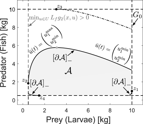
Figure 3: Admissible set for a system with interacting larvae and fish. The input realisation $\bar{u}(t)$ associated with the barrier trajectory initiating from $z_{2}$ switches at the grey point.

6 Discussion

It is interesting to note that other works in the literature that concentrate on biological applications of the viability kernel describe its boundary, and argue that it is made up of special integral curves of the system. A similar statement is made in the theory of barriers, the main observation being that these curves satisfy a minimum/maximum-like principle, as described in Theorem 1. In this new paradigm it can be seen that the description of the boundary is much simpler than the arguments in, for example, Bayen and Rapaport (2019).

Recall that the considered predator-prey system never has a (nontrivial) MRPI. Thus, the interpretation is that if one can control the introduction or harvesting of species, then this has to be done carefully, because there always exists an input (intervention strategy) that results in over- or under-population of a species in the future. Thus, it is vital that the population number remains in $\mathcal{A}$. Furthermore, the unique input on the boundary of $\mathcal{A}$ is always saturated, and it switches according to the statement in Proposition 3. For a given system, similar to the model of the CEA system presented in this work, the proposed method can be used to set up the initial population as well as intervention strategies through the addition and/or removal of the species.

7 Conclusion

The main goal of this paper was to analyse CEA systems with interacting species, modelled by the Lotka-Volterra equations, to identify the admissible set and the MRPI which yields information about sustainable intervention strategies. We used the theory of barriers to determine special trajectories that define the boundaries of the admissible set and discovered new aspects, such as the nonexistence of nontrivial MRPIs in the considered constrained Lotka-Volterra model. Furthermore, we obtained conditions of the systems’ parameters that guarantees the existence of these special trajectories. We illustrated our results based on a CEA system with larve and fish as interacting species. Future research could focus on extending the results to robust admissible sets, as in Regnier and De Lara (2015), in the context of viability theory. Another interesting idea could be to analyse the sets of an extended Lotka-Volterra model that describes the effects of humans feeding one species to another.

References

- Barnosky et al. (2011) Barnosky, A.D., Matzke, N., Tomiya, S., Wogan, G.O.U., Swartz, B., Quental, T.B., Marshall, C., McGuire, J.L., Lindsey, E.L., Maguire, K.C., Mersey, B., and Ferrer, E.A. (2011). Has the earth’s sixth mass extinction already arrived? Nature, 471(7336), 51–57.
- Bayen and Rapaport (2019) Bayen, T. and Rapaport, A. (2019). Minimal time crisis versus minimum time to reach a viability kernel: A case study in the prey-predator model. Optimal Control Applications and Methods, 40(2), 330–350.
- Conrad et al. (2017) Conrad, Z., Daniel, S., and Vincent, V. (2017). Vertical farm 2.0: Designing an economically feasible vertical farm - a combined european endeavor for sustainable urban agriculture. Technical report, Association for Vertical Farming. White Paper.
- De Dona and Lévine (2013) De Dona, J.A. and Lévine, J. (2013). On barriers in state and input constrained nonlinear systems. SIAM Journal on Control and Optimization, 51(4), 3208–3234.
- De Lara and Doyen (2008) De Lara, M. and Doyen, L. (2008). Sustainable management of natural resources: mathematical models and methods. Springer Science & Business Media.
- Diener et al. (2009) Diener, S., Zurbrügg, C., and Tockner, K. (2009). Conversion of organic material by black soldier fly larvae: establishing optimal feeding rates. Waste Management & Research, 27(6), 603–610.
- Eisenack et al. (2006) Eisenack, K., Scheffran, J., and Kropp, J.P. (2006). Viability analysis of management frameworks for fisheries. Environmental Modeling & Assessment, 11(1), 69–79.
- Esterhuizen et al. (2019) Esterhuizen, W., Aschenbruck, T., and Streif, S. (2019). On maximal robust positively invariant sets in constrained nonlinear systems. arXiv:1904.01985.
- Fort et al. (2017) Fort, H., Dieguez, F., Halty, V., and Lima, J.M.S. (2017). Two examples of application of ecological modeling to agricultural production: Extensive livestock farming and overyielding in grassland mixtures. Ecological Modelling, 357, 23–34.
- Funabashi (2018) Funabashi, M. (2018). Human augmentation of ecosystems: objectives for food production and science by 2045. npj Science of Food, 2(1), 1–11.
- Getz (2012) Getz, W.M. (2012). A biomass flow approach to population models and food webs. Natural resource modeling, 25(1), 93–121.
- Gligorescu et al. (2019) Gligorescu, A., Toft, S., Hauggaard-Nielsen, H., Axelsen, J.A., and Nielsen, S.A. (2019). Development, growth and metabolic rate of hermetia illucens larvae. Journal of Applied Entomology, 143(8), 875–881.
- Graham et al. (2007) Graham, D.W., Knapp, C.W., Van Vleck, E.S., Bloor, K., Lane, T.B., and Graham, C. (2007). Experimental demonstration of chaotic instability in biological nitrification. 385–393.
- Martinet and Doyen (2007) Martinet, V. and Doyen, L. (2007). Sustainability of an economy with an exhaustible resource: A viable control approach. Resource and energy economics, 29(1), 17–39.
- Rana et al. (2015) Rana, K.S., Salam, M., Hashem, S., and Islam, M.A. (2015). Development of black soldier fly larvae production technique as an alternate fish feed. International Journal of Research in Fisheries and Aquaculture, 5(1), 41–47.
- Regnier and De Lara (2015) Regnier, E. and De Lara, M. (2015). Robust viable analysis of a harvested ecosystem model. Environmental Modeling & Assessment, 20(6), 687–698.
- Schmidt et al. (2014) Schmidt, J.M., Barney, S.K., Williams, M.A., Bessin, R.T., Coolong, T.W., and Harwood, J.D. (2014). Predator–prey trophic relationships in response to organic management practices. Molecular Ecology, 23(15), 3777–3789.
- Stamer et al. (2014) Stamer, A., Wessels, S., Neidigk, R., and Hoerstgen-Schwark, G. (2014). Black soldier fly (hermetia illucens) larvae-meal as an example for a new feed ingredients’ class in aquaculture diets. Proceedings of the 4th ISOFAR Scientific Conference.
- Terpstra (2015) Terpstra, A.H. (2015). Feeding and growth parameters of the tilapia (oreochromis niloticus) in the body weight range from newly hatched larvae (about 5 mgrams) to about 700 grams. Growth, 600, 800.
- Zhang et al. (2000) Zhang, X., Chen, L., and Neumann, A.U. (2000). The stage-structured predator–prey model and optimal harvesting policy. Mathematical Biosciences, 168(2), 201–210.