aphBO-2GP-3B: A budgeted asynchronous parallel multi-acquisition functions for constrained Bayesian optimization on high-performing computing architecture

Abstract

High-fidelity complex engineering simulations are often predictive, but also computationally expensive and often require substantial computational efforts. The mitigation of computational burden is usually enabled through parallelism in high-performance cluster (HPC) architecture. Optimization problems associated with these applications is a challenging problem due to the high computational cost of the high-fidelity simulations. In this paper, an asynchronous parallel constrained Bayesian optimization method is proposed to efficiently solve the computationally-expensive simulation-based optimization problems on the HPC platform, with a budgeted computational resource, where the maximum number of simulations is a constant. The advantage of this method are three-fold. First, the efficiency of the Bayesian optimization is improved, where multiple input locations are evaluated massively parallel in an asynchronous manner to accelerate the optimization convergence with respect to physical runtime. This efficiency feature is further improved so that when each of the inputs is finished, another input is queried without waiting for the whole batch to complete. Second, the proposed method can handle both known and unknown constraints. Third, the proposed method samples several acquisition functions based on their rewards using a modified GP-Hedge scheme. The proposed framework is termed aphBO-2GP-3B, which means asynchronous parallel hedge Bayesian optimization with two Gaussian processes and three batches. The numerical performance of the proposed framework aphBO-2GP-3B is comprehensively benchmarked using 16 numerical examples, compared against other 6 parallel Bayesian optimization variants and 1 parallel Monte Carlo as a baseline, and demonstrated using two real-world high-fidelity expensive industrial applications. The first engineering application is based on finite element analysis (FEA) and the second one is based on computational fluid dynamics (CFD) simulations.

In memory of John Michael Furlan.

1 Introduction

Bayesian optimization (BO) is a well-known effective surrogate-based optimization methodology for high-fidelity complex simulations [1]. The efficiency is mainly achieved through a Gaussian process (GP) surrogate model to approximate the response surface, as the optimization process advances. The GP model incorporates search history and updates sequentially as soon as new information is available. The traditional BO approach relies on an underlying Gaussian process (GP) to model the response surface and utilizes an acquisition function to locate the most valuable input point for the next sampling location, simply by maximizing the acquisition function. However, like any other sequential optimization method, the traditional sequential BO approach suffers from the computational cost of the simulation, in which high-fidelity simulations typically correspond to high computational cost. Furthermore, in practical settings, the simulation does not always return a definite output. Such situation can occur in any real-world engineering application if the mesh is irregular, the solver is ill-conditioned, or the simulation is hung indefinitely. These problems, which are common but have not been adequately addressed, pose a challenge for any applications of BO on two fronts: parallel optimization and optimization under unknown constraints.

Direct applications of BO are usually limited in terms of efficiency and robustness. Enabling parallelism in BO is critical in improving efficiency of the traditional BO approach, because better optimization solution can be obtained within a shorter amount of physical time. The parallelism in optimization further enhances the parallelism of complex simulations on a high-performance computing (HPC) platform, because it is independent of the parallelism of the simulation packages, thus the speedup is improved linearly in theory. The main reason is that with more samples, the underlying GP can converge faster in approximating the response and this can accelerate the optimization process. Naïve applications of the traditional BO method often faces a challenge when the simulation does not return the output, because the underlying GP model requires both inputs and outputs to construct the response surface. Due to the broad scope of BO methods, in Section 2, the literature review for the traditional BO method and its variants are discussed, including a brief introduction to BO, application to constrained problems, and its parallel extension.

In this work, the aphBO-2GP-3B framework is developed as an extension to our previous pBO-2GP-3B framework [2], to efficiently solve a simulation-based constrained optimization on HPC platforms, where the maximum number of simulations is fixed as a constant. Similar to the pBO-2GP-3B, the aphBO-2GP-3B framework relies on three batches, where priorities are assigned differently depending on the batch, with more focus emphasized on the batch that optimizes the problem. Supporting the aphBO-2GP-3B framework are two distinct GP models, where the first GP corresponds to the objective function, whereas the second GP corresponds to the unknown constraints of the simulations. The known constraints are formulated as inequality constraints, which are then penalized directly into the acquisition function when searching for the next sampling location. Compared to the pBO-2GP-3B approach, the proposed aphBO-2GP-3B framework supersedes in two aspects. First, the parallelization is implemented in an asynchronous manner, which completely relaxes the synchronous batch-sequential parallel conditions, to further improve the efficiency of the parallel BO method. Second, multiple acquisition functions are considered in the main batch and sampled based on its reward according to the GP-Hedge scheme [3].

The aphBO-2GP-3B framework presents a practical implementation of parallel constrained BO method that is highly applicable for many computationally expensive high-fidelity engineering simulations on the HPC platform. The advantage of the current approach is the improvement of both efficiency and robustness of the traditional BO method. The efficiency of the aphBO-2GP-3B is enabled through several approaches within the framework, including sampling multiple acquisition functions and the implementation of highly asynchronous parallel feature. The robustness of the aphBO-2GP-3B is achieved through coupling with a probabilistic binary classifier to distinguish feasible and infeasible regions. In this paper, we consider a general constrained optimization problem with focus given to problems with computationally expensive high-fidelity engineering simulation.

The remainder of the paper is organized as follows. Section 2 provides the literature review for GP and BO with different relevant extensions, including known constrained, unknown constrained, synchronous batch-sequential parallel, and asynchronous parallel. In Section 3, the proposed aphBO-2GP-3B framework is described and discussed in details. Section 5 presents the first application of the aphBO-2GP-3B framework for thermo-mechanical flip-chip design optimization based on finite element analysis (FEA) simulation. Section 6 presents the second application of the aphBO-2GP-3B framework for slurry pump casing design optimization using multiphase 3D computational fluid dynamics (CFD) simulation. Section 7 discusses and Section 8 concludes the paper, respectively.

2 Related works

In this section, the literature review related to BO method is discussed. Section 2.1 provides a brief formulation on the GP formulation. Section 2.2 describes several commonly used acquisition functions in BO method. Section 2.3.1 and Section 2.3.2 discuss currently existing approaches in BO literature to handle known and unknown constraints, respectively. Section 2.4 presents the batch parallel approach to parallelize BO. In particular, Section 2.4.1 and Section 2.4.2 describe the synchronous batch-sequential parallel and asynchronous parallel approaches, respectively.

2.1 Gaussian process & Bayesian optimization

Comprehensive and critical review studies are provided by Brochu et al. [4], Shahriari et al. [5], Frazier [6], and Jones et al. [1] for BO method and its variants. A brief introduction to GP is discussed, as the GP surrogate model plays a critical role in BO methods. We adopt the notation from Shahriari et al. [5] and Tran et al. [7, 8, 9, 2, 10, 11, 12] for its clarity and consistency. In this formulation, we treat the optimization problem in the maximization settings,

$$\operatorname*{argmax}_{x\in\mathcal{X}}f(x)$$ (1)

subject to a set of nonlinear inequalities constraints

$$\lambda_{j}(\bm{x})\leq 0,\quad 1\leq j\leq J.$$ (2)

Assume that $\displaystyle f$ is a function of $\displaystyle\bm{x}$, where $\displaystyle\bm{x}\in\mathcal{X}$ is the $\displaystyle d$-dimensional input. A $\displaystyle\mathcal{GP}(\mu_{0},k)$ is a nonparametric model over functions $\displaystyle f$, which is fully characterized by the prior mean functions $\displaystyle\mu_{0}(x):\mathcal{X}\mapsto\mathbb{R}$ and the positive-definite kernel, or covariance function $\displaystyle k:\mathcal{X}\times\mathcal{X}\mapsto\mathbb{R}$. In GP regression, it is assumed that $\displaystyle\bm{f}=f_{1:n}$ is jointly Gaussian, and the observation $\displaystyle y$ is normally distributed given $\displaystyle f$, leading to

$$\bm{f}|\bm{x}\sim\mathcal{N}(\bm{m},\bm{K}),$$ (3)

$$\bm{y}|\bm{f},\sigma^{2}\sim\mathcal{N}(\bm{f},\sigma^{2}\bm{I}),$$ (4)

where $\displaystyle m_{i}:=\mu(\bm{x}_{i})$, and $\displaystyle K_{i,j}:=k(\bm{x}_{i},\bm{x_{j}})$. Equation 3 describes the prior distribution induced by the GP.

The covariance kernel $\displaystyle k(\cdot,\cdot)$ is a choice of modeling covariance between inputs, depending on the smoothness assumption of $\displaystyle f$. The family of Matérn kernels is arguably one of the most popular choices for kernels, offering a broad class for stationary kernels which are controlled by a smoothness parameter $\displaystyle\nu>0$ (cf. Section 4.2, [13]), including the square-exponential ($\displaystyle\nu\to\infty$) and exponential $\displaystyle(\nu=1/2)$ kernels. The Matérn kernels are described as

$$\bm{K}_{i,j}=k(\bm{x}_{i},\bm{x}_{j})=\theta_{0}^{2}\frac{2^{1-\nu}}{\Gamma(\nu)}(\sqrt{2\nu}r)^{\nu}K_{\nu}(\sqrt{2\nu}r),$$ (5)

where $\displaystyle K_{\nu}$ is a modified Bessel fuction of the second kind and order $\displaystyle\nu$. Common kernels for GP include [5]

• $\displaystyle\nu=1/2:k_{\text{Mat{\'{e}}rn}1}(\bm{x},\bm{x^{\prime}})=\theta_{0}^{2}\exp{(-r)}$ (also known as exponential kernel),

• $\displaystyle\nu=3/2:k_{\text{Mat{\'{e}}rn}3}(\bm{x},\bm{x^{\prime}})=\theta_{0}^{2}\exp{(-\sqrt{3}r)}(1+\sqrt{3}r)$,

• $\displaystyle\nu=5/2:k_{\text{Mat{\'{e}}rn}5}(\bm{x},\bm{x^{\prime}})=\theta_{0}^{2}\exp{(-\sqrt{5}r)}\left(1+\sqrt{5}r+\frac{5}{3}r^{2}\right)$,

• $\displaystyle\nu\to\infty:k_{\text{sq-exp}}(\bm{x},\bm{x^{\prime}})=\theta_{0}^{2}\exp{\left(-\frac{r^{2}}{2}\right)}$ (also known as square exponential or automatic relevance determination kernel),

where $\displaystyle r^{2}=(\bm{x}-\bm{x}^{\prime})\bm{\Lambda}(\bm{x}-\bm{x}^{\prime})$, and $\displaystyle\bm{\Lambda}$ is a diagonal matrix of $\displaystyle d$ squared length scale $\displaystyle\theta_{i}$.

Let the dataset $\displaystyle\mathcal{D}={(\bm{x}_{i},y_{i})}_{i=1}^{n}$ denote a collection of $\displaystyle n$ noisy observations and $\displaystyle\bm{x}$ denote an arbitrary input of dimension $\displaystyle d$. Under the formulation of GP, given the dataset $\displaystyle\mathcal{D}_{n}$, the prediction for an unknown arbitrary point is characterized by the posterior Gaussian distribution, which can be described by the posterior mean and posterior variance functions, respectively as

$$\mu_{n}(\bm{x})=\mu_{0}(\bm{x})+\bm{k}(\bm{x})^{T}(\bm{K}+\sigma^{2}\bm{I})^{-1}(\bm{y}-\bm{m}),$$ (6)

and

$$\sigma_{n}^{2}=k(\bm{x},\bm{x})-\bm{k}(\bm{x})^{T}(\bm{K}+\sigma^{2}\bm{I})^{-1}\bm{k}(\bm{x}),$$ (7)

where $\displaystyle\bm{k}(\bm{x})$ is the covariance vector between the query point $\displaystyle\bm{x}$ and $\displaystyle\bm{x}_{1:n}$. The main drawback of GP formulation is its scalability $\displaystyle\mathcal{O}(n^{3})$ that originates from the computation of the inverse of the covariance matrix $\displaystyle\bm{K}$. Connection from GP to convolution neural network has been proposed where it is proved to be theoretically equivalent to single layer with infinite width [14] or infinite convolutional filters [15].

2.2 Acquisition function

In the traditional BO method, which is sequential, the GP model is constructed for the objective function, and the next sampling location is determined by maximizing the acquisition function based on the constructed GP. This acquisition function is evaluated based on the underlying GP surrogate model, thus converting the cost of evaluating the real simulation to the cost of evaluating on the GP model. Compared between the two, the later is much more computationally appealing because it is semi-analytical. The acquisition function must balance between the exploitation and exploration flavors of the BO method. Too much exploitation would drive the numerical solution to a local minima, whereas too much exploration would make BO an inefficient optimization method. We review three main acquisition functions that are typically used in the literature: the probability of improvement (PI), the expected improvement (EI), and the upper-confident bounds (UCB).

Denote $\displaystyle\mu(\bm{x})$, $\displaystyle\sigma^{2}(\bm{x})$, and $\displaystyle\theta(\bm{x})$ as the posterior mean, the posterior variance, and the hyper-parameters of the objective GP model, respectively. $\displaystyle\theta(\bm{x})$ is obtained by maximizing the log likelihood estimation over a plausible chosen range. Let $\displaystyle\phi(\cdot)$ and $\displaystyle\Phi(\cdot)$ be the standard normal probability distribution function and cumulative distribution function, respectively, and $\displaystyle\bm{x}_{\text{best}}=\operatorname*{argmax}_{1\leq i\leq n}f(\bm{x}_{i})$ be the best-so-far sample. Rigorously, the acquisition function should be written as $\displaystyle a(\bm{x};\{\bm{x}_{i},y_{i}\}_{i=1}^{n},\theta)$, but for the sake of simplicity, we drop the dependence on the observations and simply write as $\displaystyle a(\bm{x})$ and $\displaystyle\mathbb{E}(\cdot)$ is implicitly understood as $\displaystyle\mathbb{E}_{y\sim p(y|\mathcal{D}_{n},\bm{x})}(\cdot)$ unless specified otherwise.

The PI acquisition function [16] is defined as

$$a_{\text{PI}}(\bm{x})=\text{Pr}(y>f(\bm{x}_{\text{best}}))={\mathbb{E}\left[\mathbbm{1}_{y>f(\bm{x}_{\text{best}})}\right]}=\Phi(\gamma(\bm{x})),$$ (8)

where

$$\gamma(\bm{x})=\frac{\mu(\bm{x})-f(\bm{x}_{\text{best}})}{\sigma(\bm{x})},$$ (9)

indicates the deviation away from the best sample. The PI acquisition function is constructed based on the idea of binary utility function, where a unit reward is received if a new best-so-far sample is found, and zero otherwise.

The EI acquisition function [17, 18, 19, 20] is defined as

$$a_{\text{EI}}(\bm{x})=\sigma(\bm{x})\cdot(\gamma(\bm{x})\Phi(\gamma(\bm{x}))+\phi(\gamma(\bm{x})).$$ (10)

The EI acquisition is constructed based on an improvement utility function, where the reward is the relative difference if a new best-so-far sample is found, and zero otherwise. A closely related generalization of the EI acquisition function, called knowledge-gradient (KG) acquisition function, has been suggested in [21]. Under the assumptions of noise-free and the sampling function is restricted, the EI acquisition function is recovered from the KG acquisition function. If the EI acquisition function is rewritten as

$$a_{\text{EI}}(\bm{x})={\mathbb{E}\left[\max\left(y,f(\bm{x}_{\text{best}})\right)-f(\bm{x}_{\text{best}})\right]}={\mathbb{E}\left[\max(y-f(\bm{x}_{\text{best}},0)\right]}={\mathbb{E}\left[(y-f(\bm{x}_{\text{best}})^{+}\right]},$$ (11)

then the KG acquisition function is expressed as

$$a_{\text{KG}}(\bm{x})={\mathbb{E}\left[\max\mu_{n+1}(\bm{x})|\bm{x}_{n+1}=\bm{x}\right]}-\max(\mu_{n}(\bm{x}))$$ (12)

for one-step look-ahead acquisition function.

The UCB acquisition function [22, 23, 24] is defined as

$$a_{\text{UCB}}(\bm{x})=\mu(\bm{x})+\kappa\sigma(\bm{x}),$$ (13)

where $\displaystyle\kappa$ is a hyper-parameter describing the acquisition exploitation-exploration balance. Here, we adopt the $\displaystyle\kappa$ computation from Daniel et al. [25], where

$$\kappa=\sqrt{\nu\gamma_{n}},\quad\nu=1,\quad\gamma_{n}=2\log{\left(\frac{n^{d/2+2}\pi^{2}}{3\delta}\right)},$$ (14)

and $\displaystyle d$ is the dimensionality of the problem, and $\displaystyle\delta\in(0,1)$ [24].

Another type acquisition function is entropy-based, such as GP-PES [26, 27, 28, 29], GP-ES [30], GP-MES [31]. Since GP is collectively a distribution of functions, the distribution of the global optimum $\displaystyle\bm{x}^{*}$ can be estimated as well from sampling the GP posterior. The predictive-entropy-search (PES) can be written as

$$a_{\text{PES}}(\bm{x})=H[p(\bm{x}^{*}|\mathcal{D}_{n})]-\mathbb{E}\left[H[p(\bm{x}^{*}|\mathcal{D}\cup\{(\bm{x},y)\})]\right]=H[p(y|\mathcal{D}_{n},\bm{x})]-\mathbb{E}_{p(\bm{x}^{*}|\mathcal{D}_{n})}[H(p(y|\mathcal{D}_{n},\bm{x},\bm{x}^{*}))]$$ (15)

Wang et al. [31] proposed GP-MES acquisition function, which effectively suggests sampling $\displaystyle y^{*}$ from the 1-dimensional output space $\displaystyle\mathbb{R}$ using Gumbel distribution instead of $\displaystyle\bm{x}$ in the high-dimensional input space $\displaystyle\mathcal{X}$, i.e.

$$a_{\text{MES}}(\bm{x})=H[p(y|\mathcal{D}_{n},\bm{x})]-\mathbb{E}[H(p(y|\mathcal{D}_{n},\bm{x},y^{*}))],$$ (16)

Last but not least, since the $\displaystyle f(\bm{x})$ is Gaussian, the differential entropy can be simplified to a function of posterior variance $\displaystyle\sigma^{2}(\bm{x})$, i.e.

$$H[p(y|\mathcal{D}_{n},\bm{x})]=0.5\log\left[2\pi e(\sigma^{2}(\bm{x})+\sigma^{2})\right],$$ (17)

and thus pure exploration search which targets $\displaystyle\bm{x}$ with maximum posterior variance $\displaystyle\sigma^{2}(\bm{x})$, i.e. $\displaystyle a_{\text{PE}}(\bm{x})=\sigma^{2}(\bm{x})$ is theoretically identical with the maximum differential entropy. Interestingly, Wilson et al. [32] proposed a reparameterization of most commonly used acquisition functions in terms of deep learning convolution kernels. Connection from GP to convolution neural network has been proposed where it is proved to be theoretically equivalent to single layer with infinite width [14] or infinite convolutional filters [15].

2.3 Constraints

Digabel and Wild [33] proposed a QRAK taxonomy to classify constrained optimization problems. Conceptually speaking, there are two types of constraints: known and unknown. The known constraints can be imposed beforehand without running the simulation, and thus can be handled using a separate constraint evaluator. Usually, the known constraint evaluator is computationally cheap compared to the simulation. On the contrary, the unknown constraints cannot be accessed without running the simulations, and thus are only evaluated at the same time when the simulation is performed. The unknown constraints are more expensive to obtain and require more careful attention. A review and comparison study is performed by Parr et al. [34] for different schemes to handle constraints using both synthetic and real-world applications. Many previous works discussed below in the literature prefer to couple constraint satisfaction problems with the EI acquisition due to its consistent numerical performance.

2.3.1 Known constraints

Known-constrained optimization problems are well studied in the literature and mostly formulated as a set of inequality constraints. Gramacy and Lee [35] introduced an acquisition function based on the integrated expected conditional improvement by integrating the EI acquisition function and the probabilities of satisfying constraints over the whole space. Gramacy et al. [36] combined the EI acquisition function and augmented Lagrangian framework to convert a constrained to an unconstrained optimization problem. Zhou et al. [37] also converted a constrained multi-fidelity optimization problem to an unconstrained multi-fidelity optimization problem by adding penalty function accounting for the constraint violations. Schonlau et al. [38] proposed a constrained EI acquisition function by multiplying the EI acquisition with the probabilities to satisfy for each individual constraint. Gardner et al. [39] penalized the known constraints directly by assigning zero improvement to all infeasible points through a binary feasibility indicator function. Letham et al. [40] extended the methods of Gardner et al. [39] and Gelbart et al. [41] in a noisy experiment settings at Facebook.

2.3.2 Unknown constraints

Unknown-constrained problems are harder and did not receive enough research attention until recently. Gelbart et al. [41] proposed to threshold the probability of constraint satisfaction, where the threshold is a user-defined parameter. Hernández-Lobato et al. [27] proposed an alternative acquisition function based on GP-PES [26, 29] for constrained problems by choosing the sampling location that maximizes the expected reduction of differential entropy of the posterior. Basudhar et al. [42] used support vector machines to calculate the probability of satisfying unknown constraints and combined with the EI acquisition function. Sacher et al. [43] extended the method of Basudhar et al. [42] and combined with augmented Lagrangian approach for handling both known and unknown constraints. Lee et al. [44] coupled the random forest classifier with the EI acquisition function by multiplying the EI acquisition function with the feasible probability.

2.4 Parallelization

To accelerate the optimization process for computationally expensive applications, there are mainly two approaches. The first approach is to parallelize the applications on the HPC platform, by exploiting multi-core architecture and decomposing the domain accordingly. The limitation of this approach is that in most applications, there is always a theoretical speedup that can only be achieved theoretically by Amdahl’s law [45], posing a computational threshold for accelerating the process. Furthermore, this approach is not efficient due to the diminishing return in increasing the number of processors used on the HPC platform. The second approach is to parallelize the optimizer itself by concurrently running at multiple sampling locations. For the BO method, this is typically achieved by batch parallel approach, which a batch of sampling points are evaluated, as opposed to one single sampling location. To search for new sampling locations, one can rely on the Gaussian posterior of the outputs and condition the parallel acquisition based on the posterior.

2.4.1 Sequential batch parallel

Similar to the constrained BO problem, the EI acquisition function has been used extensively in the literature. Ginsbourger et al. [46, 47, 48], Roustant et al. [49] proposed the q-EI framework to select multiple points based on the EI acquisition function. Analytical formula is available for q-EI with the batch size $\displaystyle q$ of two, but as $\displaystyle q$ grows, it requires a numerical computation of high-dimensional integration, which can be achieved by MC. Marmin et al. [50, 51] proposed a analytical simplification for q-EI to avoid high-dimensional integration in large batch based on gradient-based ascent algorithms. Wang et al. [52] also employed a gradient-based approach but relying on infinitesimal perturbation analysis to construct a stochastic gradient estimator to simplify the high-dimensional integration in the original q-EI framework. Wang et al. [52] and Wu and Frazier [53] (q-KG) proposed a parallel version for KG acquisition function [54]. Rontsis et al. [55] proposed another acquisition function GP-OEI to reduce the computational burden of q-EI on high-dimensional space, where the lower and upper bounds are computationally tractable in high-dimensional space and showed its numerical robustness over q-EI. Snoek et al. [20] proposed an integrated EI acquisition function based on Monte Carlo (MC) sampling, called GP-EI-MCMC to construct a batch. Azimi et al. [56, 57, 58] proposed a simulation matching scheme GP-SM [56], coordinated matching scheme GP-BCM [57], and a hybrid sequential-parallel [58] to recalibrate the batch behavior to the sequential BO after a number of steps. Shah and Ghahramani [59] proposed a batch parallel GP-PES approach based on entropy acquisition function. Desautels et al. [60] proposed a batch parallel hallucination scheme, called GP-BUCB-ACUB, that combines both UCB acquisition function and kriging believer heuristic in Ginsbourger et al [46, 47]. Contal et al. [61] extended the method of Desautels et al. [60] by promoting exploration within a batch while leaving only one sampling point for exploitation. Kathuria et al. [62] and Wang et al. [63] employed the determinantal point process to propose a batch selection policy GP-DPP, and proved the expected regret bound of DPP-SAMPLE is less than the regret bound of GP-UCB-PE [61]. Daxberger and Low [64] proposed a distributed batch GP-UCB, called DP-GP-UCB to jointly optimize a batch of inputs, by formulating the batch input selection as a multi-agent distributed constraint optimization problem, as opposed to selecting the inputs of a batch one at a time, while preserving the scalability in the batch size. González et al. [65] proposed a local penalization GP-LP method to penalize the acquisition function locally with an estimated Lipschitz constant to construct a batch. Nguyen et al. [66] proposed a budgeted batch BO, termed GP-B3O, which samples the acquisition functions, then equates the number of peaks as the batch sizes and assigns sampling locations at the sampled peaks. However, most of the above-mentioned approaches are synchronous batch-sequential parallel, in the sense that at the end of each batch, all the simulations must be completed in order to move forward.

2.4.2 Asynchronous parallel

Ginsbourger et al. [67] discussed and proposed the expected EI by conditioning the EI acquisition on the busy sampling points. Janusevskis et al. [68] proposed an asynchronous multi-points EI acquisition function by estimating the progress of the available and incoming sampling locations. Letham et al. [40] also employed the q-EI framework to asynchronous parallelize in noisy environment. GP-EI-MCMC [20] can also be extended to accommodate the asynchronous parallel feature in BO. Kamiński and Szufel [69] extended the q-KG framework for asynchronous parallel BO method. Kotthaus et al. [70] proposed a resource-aware framework with different priorities, called RAMBO, that aim to reduce idle time on the computational workers through knapsack problem formulation. Kandasamy et al. [71] proposed an asynchronous parallel BO based on Thompson sampling approach [72]. Pokuri et al. [73] implemented PARyOpt package with an asynchronous function evaluator where users can impose a threshold for a batch to finish before moving to a next batch. Alvi et al. [74] further extended a locally penalization scheme to asynchronously parallel BO [65].

3 Methodology

Here, we consider the optimization problem

$$\bm{x}^{*}=\operatorname*{argmax}_{\bm{x}\in\mathcal{X}}f(\bm{x}),$$ (18)

subject to

$$\lambda_{j}(\bm{x})\leq g_{j},\quad j=1,\dots,J,$$ (19)

where $\displaystyle f$ is evaluated through a computationally expensive engineering simulation, where the output $\displaystyle f(\bm{x})$ may not exist on some subspace of the input domain $\displaystyle\mathcal{X}$. $\displaystyle\lambda_{j}(\bm{x}),1\leq j\leq J$, is a known constraint, formulated as a set of nonlinear inequality, and is cheap to evaluate. The input domain therefore can be decomposed into two disjoint regions, feasible and infeasible, as $\displaystyle\mathcal{X}=\mathcal{X}_{\text{infeasible}}\cup\mathcal{X}_{\text{feasible}}$, where the feasible region is a collection of input $\displaystyle\bm{x}$, where none of the nonlinear inequality constraints is violated, and $\displaystyle f(\bm{x})\in\mathbb{R}$ exists, and the infeasible region is the complement of the feasible region.

We further decompose the infeasible regions as the union of two subspaces, where $\displaystyle\{\bm{x}\in\mathcal{X}\quad|\quad\exists j:\quad\lambda_{j}(\bm{x})>g_{j}\}$ is the subspace where at least one known constraint is violated, and the complement is the subspace where $\displaystyle\bm{x}$ is infeasible for some unknown reasons, such as the functional evaluator $\displaystyle f(\bm{x})$ fails unexpectedly, numerical divergence in the solver is detected, or mesh creation is failed uncontrollably at the particular input $\displaystyle\bm{x}$. It is worthy to note that these two subspaces are not necessarily disjoint.

In our previous work [2], we proposed a pBO-2GP-3B framework to handle known and unknown constrained in a batch-sequential parallel manner. The current method aphBO-2GP-3B is the natural extension of the pBO-2GP-3B framework in two main directions: the implementation of the asynchronous feature, and the implementation of multi-acquisition function under the GP-Hedge scheme, as described in Hoffman et al [3]. Compared to other methods in literature, the aphBO-2GP-3B approach is more practical in several aspects.

First, the aphBO-2GP-3B approach provides a flexibility by relaxing the probabilistic binary classifier in distinguishing feasible and infeasible regions. There is no restriction in choosing the binary classifier, even though some classifiers tend to outperform others. The binary classifier can be $\displaystyle k$NN [75], AdaBoost [76], RandomForest [77], support vector machine [78] (SVM), least squares support vector machine (LSSVM) [79], GP [80], and convolutional neural network [81]. Similar to the pBO-2GP-3B, we adopted the method of Gardner et al. [39] to penalize the acquisition function where the known constraints are violated.

Second, multiple acquisition functions are considered and statistically sampled based on their performance measured by rewards. The reward handling scheme is only valid for feasible samples. This approach unifies and leverages the advantage of different acquisition functions individually, including PI, EI, and UCB.

Third, it takes advantage of HPC parallelism by parallelizing asynchronously to reduce the wait time. This is more efficient than the synchronous batch-sequential parallel BO approach because the synchronous time requirement within a batch is removed, allowing more simulations to be completed. The problem is considered in a HPC environment where the number of cores used for optimization are limited.

Similar to the GP-UCB framework [60] and kriging believer heuristic [46, 47], our approach aphBO-2GP-3B hallucinates the objective GP by assuming that the posterior means at the sampling locations are the observations until the actual observations are available. The term ”hallucination”, coined by Desautels in GP-UCB [60], describes the procedure to temporarily assign the posterior mean of the objective GP as the actual observation, in order to sample the next location. The temporary assignment of the objective function is removed once the observation at the particular sampling point is made. In the current approach, we also generalize the hallucination module for the feasibility, by temporarily assuming that the sampling location is feasible.

For the GP interpolation process, at the infeasible sampling points where the outputs do not exist, an interpolation process is employed to interpolate for the objective GP to reflect the true posterior variance $\displaystyle\sigma^{2}_{\text{objective}}=0$ at these infeasible locations $\displaystyle\bm{x}_{\text{infeasible}}$. Similar the the GP hallucination process described above, this interpolation process updates the objective GP at the infeasible locations by assigning the posterior means as the observation and re-train the objective GP; however, the infeasibility of these locations remain unchanged. Without the GP interpolation process, the objective GP does not reflect the true uncertainty at these infeasible sampling locations, i.e. a large posterior variance is attributed to these locations, whereas a small posterior variance should be attributed, indeed. In other words, the $\displaystyle\sigma^{2}_{\text{objective}}$ is available at $\displaystyle\bm{x}_{\text{infeasible}}$, while the $\displaystyle\mu_{\text{objective}}$ is not at these infeasible sampling locations. Therefore, we must update $\displaystyle\mu_{\text{objective}}$ to reflect our knowledge, by the GP interpolation process. The GP interpolation process is achieved by three steps. In the first step, the objective GP is fitted only using feasible sampling locations. In the second step, the posterior mean of the objective GP is obtained by the fitted objective GP prediction. In the third step, these posterior means are used as the actual observations to fit the objective GP again.

The aphBO-2GP-3B framework is constructed based on the extension of GP-UCB [60] and GP-UCB-PE [61] using three different batches, where each batch is assigned a different job. The first batch is called the acquisition batch $\displaystyle\mathcal{B}_{\text{acquisition}}$, where a chosen acquisition is maximized to locate the next sampling point. The main job of the first batch is to optimize the objective function. Therefore, most of the computational effort and priority is reserved for the first batch. The second batch is called the exploration batch for the objective GP $\displaystyle\mathcal{B}_{\text{explore}}$, aiming at exploring the objective GP in the most uncertain regions, where $\displaystyle\sigma^{2}_{\text{objective}}$ is high. The third batch is called the exploration batch for the classification GP $\displaystyle\mathcal{B}_{\text{exploreClassif}}$, aiming at exploring the most uncertain regions for the GP classifier. GP is one of a few binary classifiers where uncertainty associated with the prediction is quantified. For other classifiers where uncertainty is not quantified, the third batch can be simply ignored.

3.1 Constraints

The aphBO-2GP-3B framework supports both known and unknown constraints as described above.

3.1.1 Known constraints

The known constraints $\displaystyle\lambda_{j}(\bm{x})\leq g_{j}$ are evaluated before the functional evaluator $\displaystyle f$ is revoked. Consequently, we can define an indicator function for constraints satisfaction as

$$\mathcal{I}(\bm{x})=\begin{cases}0,\quad\text{ if }\exists j:\lambda_{j}(\bm{x})>g_{j},\\ 1,\quad\text{ if }\forall j:\lambda_{j}(\bm{x})\leq g_{j}.\\ \end{cases}$$ (20)

This function is also written as $\displaystyle\mathcal{I}\left(\lambda(\bm{x})\leq\bm{g}\right)$. Since the known constraints can be evaluated before evaluating the function $\displaystyle f$, the acquisition function $\displaystyle a(\bm{x})$ is penalized as zero by multiplying with the constraint indicator function $\displaystyle\mathcal{I}(\bm{x})$. The next sampling point is continuously searched until a sampling point with a non-zero acquisition function value that does not violate the known constraints is found.

3.1.2 Unknown constraints

The unknown constraints in general are harder to handle, because it requires an approximation within the BO. To distinguish between feasible and infeasible regions adaptively, we propose to couple an external binary classifier that adaptively learns as the optimization advances. The choice of the external binary classifier is left to users, but GP is recommended to utilize the third batch. Denote this classifier as $\displaystyle\text{clf}(\bm{x})$. For each point in the input space $\displaystyle\bm{x}\in\mathcal{X}$, the classifier predicts a probability mass function for the feasibility of $\displaystyle\bm{x}$ as $\displaystyle Pr(\text{clf}(\bm{x})=1)$ if $\displaystyle\bm{x}$ is feasible, and $\displaystyle Pr(\text{clf}(\bm{x})=0)$ if $\displaystyle\bm{x}$ is infeasible. It is obvious that $\displaystyle Pr(\text{clf}(\bm{x})=0)+Pr(\text{clf}(\bm{x})=1)=1$. This probability mass function can be used to condition on the acquisition function to drive the sampling points away from infeasible regions to feasible regions.

3.1.3 Combining both known and unknown constraints

The acquisition function $\displaystyle a(\bm{x})$ can be modified to reflect both known and unknown constraints. First, we incorporate the known constraints to the original acquisition function by multiplying them together as

$$a^{**}(\bm{x})=a(\bm{x})\cdot\mathcal{I}(\lambda(\bm{x})\leq\bm{g}).$$ (21)

Second, we condition the new acquisition function $\displaystyle a^{**}(\bm{x})$ on the probability mass function for the unknown function as

$$a^{***}(\bm{x})=\begin{cases}a^{**}(\bm{x}),&\text{ if }\text{clf}(\bm{x})=1,\\ 0,&\text{ if }\text{clf}(\bm{x})=0.\end{cases}$$ (22)

Taking the expectation of $\displaystyle a^{***}(\bm{x})$ on the probability mass function from the binary classifier yields

$$\begin{array}[]{lll}a^{*}(\bm{x})&=&\mathbb{E}[a^{***}(\bm{x})]\\ &=&a^{**}(\bm{x})\cdot Pr(\text{clf}(\bm{x})=1)+0\cdot Pr(\text{clf}(\bm{x})=0)\\ &=&a^{**}(\bm{x})\cdot Pr(\text{clf}(\bm{x})=1)\\ &=&a(\bm{x})\cdot\mathcal{I}(\lambda(\bm{x})\leq\bm{g})\cdot Pr(\text{clf}(\bm{x})=1),\\ \end{array}$$ (23)

The new acquisition function $\displaystyle a^{*}(\bm{x})$ is our constrained acquisition function, which is constructed by combining the original acquisition function $\displaystyle a(\bm{x})$ with the penalization for known and unknown constraints.

3.2 Asynchronous parallel

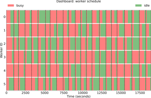
(a) Batch-sequential parallel.

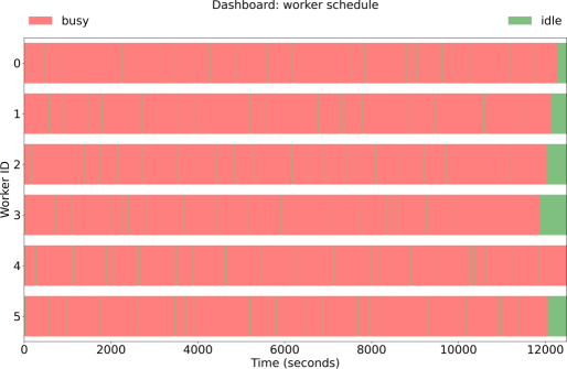
(b) Asynchronous parallel.

Figure 1: Difference between batch-sequential and asynchronous parallelizations. In batch-sequential parallelization (Figure 1(a)), all workers need to wait until the batch is finished before moving on to the next batch. In asynchronous parallelization (Figure 1(b)), all the workers receive the most up-to-date information and work independently with each other. Asynchronous parallelization is more efficient than batch-sequential parallelization because it reduces idle time for workers.

The asynchronous parallel feature is constructed based on the priority of the batch, as

$$\mathcal{B}_{\text{acquisition}}>\mathcal{B}_{\text{explore}}>\mathcal{B}_{\text{exploreClassif}},$$ (24)

because the first batch $\displaystyle\mathcal{B}_{\text{acquisition}}$ is the most important one among three batches, whenever the first batch is under filled, then the computational effort is reserved for filling the first batch. If the first batch is filled, then the second batch and the third batch is considered, respectively, according to the priority listed in Equation 24.

The asynchronous parallel feature is implemented by periodically checking if these batches are under filled. If the batches are full, then the aphBO-2GP-BO optimizer will hold until a pending sampling point is finished and some batch is under filled as a result.

3.3 Multi-acquisition function

Unified approaches considering multiple acquisition functions have been considered in the literature. For example, Shahriari proposed an entropy-based approach, called GP-EPS [82], for searching the best acquisition function within the same portfolio. In the current aphBO-2GP-3B framework, we adopt and modify the GP-Hedge scheme [3] where multiple acquisition functions are considered simultaneously for the first batch $\displaystyle\mathcal{B}_{\text{acquisition}}$. De Palma et al. [83] proposed to sample the acquisition function portfolio using Thompson sampling. After the initial sampling stage, the reward for each acquisition function is reset to zero. To locate a next sampling point in the batch $\displaystyle\mathcal{B}_{\text{acquisition}}$, first, the acquisition function is determined by sampling based on a probability mass function, where the parameters of the probability mass function correspond to their rewards, or more precisely, their numerical performance. Second, when the acquisition function is determined, the new sampling point is determined by maximizing the chosen acquisition function. Third, when a sampling point is finished querying, if the sampling point is determined to be feasible, then the reward is added into the cumulative reward of that acquisition function. The cumulative rewards are tracked throughout the optimization process. Hoffman et al. [3] proposed to choose $\displaystyle\eta_{t}=\sqrt{\frac{8\ln{k}}{n}}$ as a time-varying parameter based on Cesa-Bianchi and Lugosi [84] (Section 2.3), where $\displaystyle k$ is the number of acquisition functions considered in the GP-Hedge scheme.

Algorithm 1 Improved GP-Hedge for aphBO-2GP-3B: Inverse sampling multiple acquisition functions (modification highlighted in blue).

Input: observations $\displaystyle(y_{i},c_{i})_{i=1}^{n}$; $\displaystyle n^{*}$ acquisition functions $\displaystyle\{a_{j}\}_{j=1}^{n^{*}}$

Output: acquisition function $\displaystyle a_{j^{*}}$ sampled at iteration $\displaystyle n+1$ based on gains and rewards and the next sampling point $\displaystyle\bm{x}^{*}$

1:$\displaystyle\eta_{n}\leftarrow\sqrt{\frac{8\ln{k}}{n}}$ $\displaystyle\triangleright$ set scaling parameters for rewards (cf. [3]): $\displaystyle\eta\in\mathbb{R}^{+}$

2:$\displaystyle g_{0}^{j}\leftarrow 0$ for $\displaystyle 1\leq j\leq n^{*}$ $\displaystyle\triangleright$ initialize; $\displaystyle n^{*}$: number of acquisition functions

3:for $\displaystyle i=1,2,\dots,n$ do

4:     if  $\displaystyle\bm{x}_{i}$ feasible, $\displaystyle y_{i}$ is best-so-far  then $\displaystyle\triangleright$ modification for constrained problems

5:           $\displaystyle r^{j}_{i}\leftarrow 1$ for $\displaystyle a_{j}$ at iteration $\displaystyle i$ $\displaystyle\triangleright$ receive reward (original [3]: $\displaystyle r^{i}_{t}\leftarrow\mu(\bm{x}_{i})$)

6:     else

7:          $\displaystyle r^{j}_{i}\leftarrow 0$ $\displaystyle\triangleright$ no rewards if not feasible or not best-so-far

8:     end if

9:      $\displaystyle g^{j}_{i}\leftarrow g^{j}_{i-1}+r^{j}_{i}$ $\displaystyle\triangleright$ update gains

10:end for

11:for $\displaystyle 1\leq j\leq n^{*}$ do

12:     $\displaystyle p_{n+1}(j)\leftarrow\frac{\exp(\eta g^{j}_{n})}{\sum_{j=1}^{n^{*}}\exp(\eta g^{j}_{n})}$ $\displaystyle\triangleright$ normalize p.m.f. of $\displaystyle a_{j}$’s

13:end for

14:determine the acquisition function $\displaystyle a_{j^{*}}$

15:locate the next sampling point $\displaystyle\bm{x}^{*}\leftarrow\operatorname*{argmax}_{\bm{x}}a_{j^{*}}(\bm{x}|\mathcal{D}_{n})$ $\displaystyle\triangleright$ locate $\displaystyle\bm{x}^{*}$

3.4 Implementation and Summary

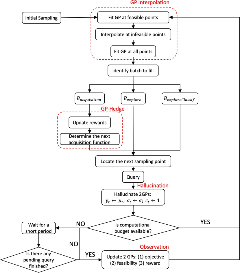
Figure 2: The aphBO-2GP-3BO flow chart. At any given time if the computational resource is available, the GP interpolation module updates the objective GP $\displaystyle\mathcal{GP}_{\text{objective}}$ by hallucinating at points that are either (a) being queried or (b) have been queried but are infeasible. Once $\displaystyle\mathcal{GP}_{\text{objective}}$ finishes updating, one sampling point is assigned to the batch according to its priority, with descending priority given to $\displaystyle\mathcal{B}_{\text{acquisition}}$, to $\displaystyle\mathcal{B}_{\text{explore}}$, to $\displaystyle\mathcal{B}_{\text{exploreClassif}}$. For the batch $\displaystyle\mathcal{B}_{\text{acquisition}}$, the rewards is updated to sample the acquisition function, which can be PI, EI, or UCB by GP-Hedge scheme. Once the acquisition function is determined, the next sampling point is located and then queried. $\displaystyle\mathcal{GP}_{\text{objective}}$ is then hallucinated again at the queried sampling point. If there is available computational budget, the loop returns to GP interpolation module; otherwise, the algorithm waits at least one query is finished.

The aphBO-2GP-3B framework is summarized in Algorithm 2. The current GP implementation is built upon modified MATLAB DACE [85] and ooDACE [86, 87, 88, 89] toolboxes. The CMA-ES method is employed [90, 91] to maximize the acquisition function and locate the next sampling point. Python scripts are devised as an interface between the aphBO-2GP-3BO in MATLAB and the actual application. After a sampling location is queried, the optimizer checks if all the batches have been filled or if there is any pending query has been completed. If there is any batch that is not filled completely, then it will be filled according to the order described in Equation 24. The aphBO-2GP optimizer then moves forward, assuming the posterior mean is the observation and continues to search for new sampling locations. If all the batches are full, then the optimizer simply waits. If there is any pending query that has been completed, then the results including objective function, feasibility, reward, are updated simultaneously, followed by the GP interpolation module before locating a new sampling point. Figure 2 presents the flowchart for aphBO-2GP-3BO framework. The GP-Hedge scheme, the GP interpolation module, and the hallucination module are highlighted to emphasize their importance.

Algorithm 2 aphBO-2GP-3B algorithm.

Input: dataset $\displaystyle\mathcal{D}_{n}$ consisting of input, observation, feasibility $\displaystyle(\bm{x},y_{i},c_{i})_{i=1}^{n}$

Input: objective $\displaystyle\mathcal{GP}(\bm{x},y_{i})_{i=1}^{n}$, and classification $\displaystyle\mathcal{GP}(\bm{x},c_{i})_{i=1}^{n}$

1:while convergence criteria not met do

2:     while number of queries $\displaystyle\not<\mathcal{B}_{\text{budget}}$ do $\displaystyle\triangleright$ wait indefinitely for available resource

3:         check periodically if there is available computational resource to use

4:     end while

5:     update input/output/feasible/complete for all cases $\displaystyle\triangleright$ update; if not complete then hallucinate, i.e. $\displaystyle y_{i}\leftarrow\mu(\bm{x}_{i}),\sigma_{i}^{2}\leftarrow\sigma^{2},c_{i}\leftarrow$ feasible

6:     update/augment dataset $\displaystyle\mathcal{D}_{n+1}=\{\mathcal{D}_{n},(\bm{x}^{(B)}_{n+1},y^{(B)}_{n+1},c^{(B)}_{n+1})\}$ $\displaystyle\triangleright$ update

7:     interpolate 2GPs $\displaystyle\triangleright$ update/hallucinate 2GPs

8:      construct $\displaystyle\mathcal{GP}_{\text{objective}}$ $\displaystyle\triangleright$ hallucinate $\displaystyle\mathcal{GP}_{\text{objective}}$

9:       construct $\displaystyle\mathcal{GP}_{\text{objective}}(\bm{x}_{i},y_{i}|c_{i}=\text{feasible})$ for feasible points

10:       hallucinate $\displaystyle\mathcal{GP}_{\text{objective}}$, i.e. $\displaystyle y_{i}\leftarrow\mu_{i},\sigma_{i}^{2}\leftarrow\sigma^{2}$, at infeasible points $\displaystyle c_{i}=\text{infeasible}$

11:       reconstruct $\displaystyle\mathcal{GP}_{\text{objective}}$ using both feasible and infeasible points

12:      construct $\displaystyle\mathcal{GP}_{\text{classification}}(\bm{x}_{i},c_{i})$ $\displaystyle\triangleright$ hallucinate $\displaystyle\mathcal{GP}_{\text{classification}}$

13:     identify which batch needs filling $\displaystyle\triangleright$ get batch type

14:     locate the next sampling location for the selected batch $\displaystyle\triangleright$ find sampling location

15:     update/hallucinate 2GPs

16:      acquisition:

17:       compute rewards for each acquisition function $\displaystyle\triangleright$ GP-Hedge (Alg. 1)

18:       sample acquisition function portfolio $\displaystyle\triangleright$ GP-Hedge (Alg. 1)

19:       locate the next sampling point with the sampled acquisition function

20:      exploration:

21:       locate the next sampling location where $\displaystyle\sigma_{\text{objective}}^{2}$ is maximized

22:      classification

23:       locate the next sampling location where $\displaystyle\sigma_{\text{classification}}^{2}$ is maximized

24:     query objective function for objective $\displaystyle y^{(B)}_{n+1}$ and feasibility $\displaystyle c^{(B)}_{n+1}$ $\displaystyle\triangleright$ query

25:     update number of queries += 1 $\displaystyle\triangleright$ increase the number of busy workers

26:end while

4 Numerical benchmark

In this section, we benchmark the aphBO-2GP-3B framework by comparing its with two of its main variants: the synchronous batch-sequential parallel pBO-2GP-3B [2] with PI, EI, UCB acquisition functions and the non-GP-Hedge asynchronous parallel apBO-2GP-3B with PI, EI, UCB acquisition functions. To augment the comparison, we also provide the numerical performance of the sequential BO and sequential Monte Carlo random search. The implementations of the testing functions used are publicly available [92] in both MATLAB and R, where R scripts are used in our benchmark. We investigate their performance with respect to both the physical wall-clock time and the number of evaluations. To simulate the random behaviors of real-world applications in terms of computational time, we append a uniformly distributed random waiting time after the functional evaluation is completed, i.e. $\displaystyle t^{*}\sim\mathcal{U}(\underline{t},\overline{t})$, where $\displaystyle\underline{t}=30$ s and $\displaystyle\overline{t}=900$ s. We compare 6 different variants of parallel BO methods, including

• pBO-2GP-3BO with UCB, EI, and PI acquisition functions [2] (the synchronous batch-sequential parallel),

• apBO-2GP-3BO – without GP-Hedge, with UCB, EI, and PI acquisition functions (the asynchronous parallel without GP-Hedge),

• aphBO-2GP-3BO – with GP-Hedge (the asynchronous parallel with GP-Hedge),

• asynchronous parallel Monte Carlo random search as a baseline,

where each method is repeated 5 times. To be fair, all benchmark runs are performed on the same workstation with Ubuntu 18.04.4 LTS, with AMD A10-6700 APU CPU and 16GB of memory. Furthermore, in order to avoid the complication of benchmarking on a relatively less capable workstation, the waiting time is relatively long so that running the optimizer does not have a significant impact on the CPU as well as the physical memory. The list of name, dimensionality, batch sizes, function form, and global minimum of benchmark functions are as follows.

• eggholder (2d): batch size = (2,2,0): max iteration = 80

  $$f(\bm{x})=-(x_{2}+47)\sin\left(\left|x_{2}+\frac{x_{1}}{2}+47\right|\right)-x_{1}\sin\left(\left|x_{1}-(x_{2}+47)\right|\right)$$ (25)

  on $\displaystyle x_{i}\in[-512,512]$ for $\displaystyle i=1,2$. Global minimum $\displaystyle f(\bm{x^{*}})=-959.6407$ at $\displaystyle\bm{x^{*}}=(512,404.2319)$.

• three-hump camel (2d): batch size = (2,2,0): max iteration = 80

  $$f(\bm{x})=2x_{1}^{2}-1.05x_{1}^{4}+\frac{x_{1}^{6}}{6}+x_{1}x_{2}+x_{2}^{2}$$ (26)

  on the domain of $\displaystyle x_{i}\in[-5,5]$ for $\displaystyle i=1,2$. Global minimum $\displaystyle f(\bm{x^{*}})=0$ at $\displaystyle\bm{x^{*}}=(0,0)$.

• six-hump camel (2d): batch size = (3,1,0): max iteration = 80

  $$f(\bm{x})=\left(4-2.1x_{1}^{2}+\frac{x_{1}^{4}}{3}\right)x_{1}^{2}+x_{1}x_{2}+(-4+4x_{2}^{2})x_{2}^{2}$$ (27)

  on the domain of $\displaystyle\bm{x}\in[-3,3]\times[-2,2]$. Global minimum $\displaystyle f(\bm{x^{*}})=-1.0316$ at $\displaystyle\bm{x^{*}}=(-0.0898,0.7126)$.

• hartmann (3d): batch size = (3,3,0): max iteration = 150

  $$f(\bm{x})=-\sum_{i=1}^{4}\alpha_{i}\exp\left(-\sum_{j=1}^{3}A_{ij}(x_{j}-P_{ij})^{2}\right),$$ (28)

  where $\displaystyle\bm{A}=\begin{pmatrix}3.0&10&30\\ 0.1&10&35\\ 3.0&10&30\\ 0.1&10&35\end{pmatrix}$, $\displaystyle\bm{P}=10^{-4}\begin{pmatrix}3689&1170&2673\\ 4699&4387&7470\\ 1091&8732&5547\\ 381&5743&8828\end{pmatrix}$, and $\displaystyle\alpha=(1.0,1.2,3.0,3.2)^{T}$ on the domain of $\displaystyle[0,1]^{3}$. Global minimum $\displaystyle f(\bm{x^{*}})=-3.86278$ at $\displaystyle\bm{x^{*}}=(0.114614,0.555649,0.852547)$.

• hartmann (4d): batch size = (4,4,0): max iteration = 160

  $$f(\bm{x})=\frac{1}{0.839}\left[1.1-\sum_{i=1}^{4}\alpha_{i}\exp\left(-\sum_{j=4}^{3}A_{ij}(x_{j}-P_{ij})^{2}\right)\right],$$ (29)

  where $\displaystyle\bm{A}=\begin{pmatrix}10&3&17&3.50&1.7&8\\ 0.05&10&17&0.1&8&14\\ 3&3.5&1.7&10&17&8\\ 17&8&0.05&10&0.1&14\end{pmatrix}$, $\displaystyle\bm{P}=10^{-4}\begin{pmatrix}1312&1696&5569&124&8283&5886\\ 2329&4135&8307&3736&1004&9991\\ 2348&1451&3522&2883&3047&6650\\ 4047&8828&8732&5743&1091&381\end{pmatrix}$, and $\displaystyle\alpha=(1.0,1.2,3.0,3.2)^{T}$ on the domain of $\displaystyle[0,1]^{4}$.

• ackley (free d) (5d): batch size = (6,4,0): max iteration = 200

  $$f(\bm{x})=-a\exp\left(-b\sqrt{\frac{1}{d}\sum_{i=1}^{d}x_{i}^{2}}\right)-\exp\left(\frac{1}{d}\sum_{i=1}^{d}\cos(cx_{i})\right)+a+\exp(1),$$ (30)

  where $\displaystyle a=20,b=0.2,c=2\pi$, on $\displaystyle[-32.768,+32.768]^{d}$. Global minimum $\displaystyle f(\bm{x^{*}})=0$ at $\displaystyle\bm{x^{*}}=(0,\dots,0)$.

• hartmann (6d): batch size = (5,5,0): max iteration = 300

  $$f(\bm{x})=-\sum_{i=1}^{4}\alpha_{i}\exp\left(-\sum_{j=6}^{3}A_{ij}(x_{j}-P_{ij})^{2}\right),$$ (31)

  where $\displaystyle\bm{A}=\begin{pmatrix}10&3&17&3.50&1.7&8\\ 0.05&10&17&0.1&8&14\\ 3&3.5&1.7&10&17&8\\ 17&8&0.05&10&0.1&14\end{pmatrix}$, $\displaystyle\bm{P}=10^{-4}\begin{pmatrix}1312&1696&5569&124&8283&5886\\ 2329&4135&8307&3736&1004&9991\\ 2348&1451&3522&2883&3047&6650\\ 4047&8828&8732&5743&1091&381\end{pmatrix}$, and $\displaystyle\alpha=(1.0,1.2,3.0,3.2)^{T}$ on the domain of $\displaystyle[0,1]^{4}$. Global minimum $\displaystyle f(\bm{x^{*}})=-3.32237$ at $\displaystyle\bm{x^{*}}=(0.20169,0.150011,0.476874,0.275332,0.311652,0.6573)$.

• michalewicz (free d) (10d): batch size = (5,5,0): max iteration = 400

  $$f(\bm{x})=-\sum_{i=1}^{d}\sin(x_{i})\sin^{2m}\left(\frac{ix_{i}^{2}}{\pi}\right),$$ (32)

  on the domain of $\displaystyle[0,\pi]^{d}$.

• perm0db (free d) (80d): batch size = (6,4,0): max iteration = 400

  $$f(\bm{x})=\sum_{i=1}^{d}\left(\sum_{j=1}^{d}(j+\beta)\left(x_{j}^{i}-\frac{1}{j^{i}}\right)\right)^{2},$$ (33)

  on the domain of $\displaystyle[-d,d]^{d}$. Global minimum $\displaystyle f(\bm{x^{*}})=0$ at $\displaystyle\bm{x^{*}}=\left(\frac{1}{1},\frac{1}{2},\dots,\frac{1}{d}\right)$.

• rosenbrock (free d) (20d): batch size = (6,4,0): max iteration = 400

  $$f(\bm{x})=\sum_{i=1}^{d-1}\left[100(x_{i+1}-x_{i}^{2})^{2}+(x_{i}-1)^{2}\right],$$ (34)

  on the domain of $\displaystyle[-5,10]^{d}$. Global minimum $\displaystyle f(\bm{x^{*}})=0$ at $\displaystyle\bm{x^{*}}=(1,\dots,1)$.

• dixon-price (free d) (25d): batch size = (7,7,0): max iteration = 480

  $$f(\bm{x})=(x_{1}-1)^{2}+\sum_{i=2}^{d}i(2x_{i}^{2}-x_{i-1})^{2}$$ (35)

  on the domain of $\displaystyle[-10,10]^{d}$. Global minimum $\displaystyle f(\bm{x^{*}})=0$ at $\displaystyle x_{i}=2^{-\frac{2^{i}-2}{2^{i}}}$ for all $\displaystyle 1\leq i\leq d$.

• trid (free d) (30d): batch size = (6,4,0): max iteration = 400

  $$f(\bm{x})=\sum_{i=1}^{d}(x_{i}-1)^{2}-\sum_{i=2}^{d}x_{i}x_{i-1},$$ (36)

  on the domain of $\displaystyle[-d^{2},d^{2}]$. Global minimum $\displaystyle f(\bm{x^{*}})=-d(d+4)(d-1)/6$ at $\displaystyle x_{i}=i(d+1-i)$ for all $\displaystyle 1\leq i\leq d$.

• sumsqu (free d) (40d): batch size = (6,4,0): max iteration = 400

  $$f(\bm{x})=\sum_{i=1}ix_{i}^{2},$$ (37)

  on the domain of $\displaystyle[-5.12,5.12]^{d}$. Global minimum $\displaystyle f(\bm{x^{*}})=0$ at $\displaystyle\bm{x^{*}}=(0,\dots,0)$.

• sumpow (free d) (50d): batch size = (6,4,0): max iteration = 400

  $$f(\bm{x})=\sum_{i=1}^{d}|x_{i}|^{i+1},$$ (38)

  on the domain of $\displaystyle[-1,1]^{d}$. Global minimum $\displaystyle f(\bm{x^{*}})=0$ at $\displaystyle\bm{x^{*}}=(0,\dots,0)$.

• spheref (free d) (60d): batch size = (6,4,0): max iteration = 400

  $$f(\bm{x})=\sum_{i=1}^{d}x_{i}^{2},$$ (39)

  on the domain of $\displaystyle[-5.12,5.12]^{d}$. Global minimum $\displaystyle f(\bm{x^{*}})=0$ at $\displaystyle\bm{x^{*}}=(0,\dots,0)$.

• rothyp (free d) (70d): batch size = (6,4,0): max iteration = 400

  $$f(\bm{x})=\sum_{i=1}^{d}\sum_{j=1}^{i}x_{j}^{2},$$ (40)

  on the domain of $\displaystyle[-65.536,65.536]^{d}$. Global minimum $\displaystyle f(\bm{x^{*}})=0$ at $\displaystyle\bm{x^{*}}=(0,\dots,0)$.

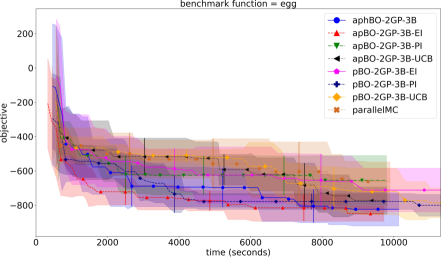
(a) Benchmark by physical wall-clock time.

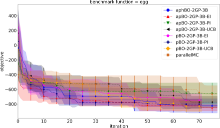
(b) Benchmark by iteration.

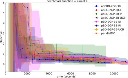
(c) Benchmark by physical wall-clock time.

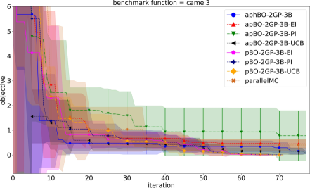
(d) Benchmark by iteration.

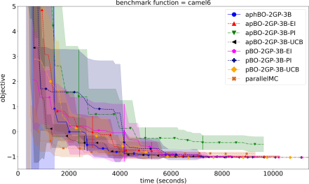
(e) Benchmark by physical wall-clock time.

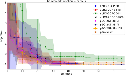
(f) Benchmark by iteration.

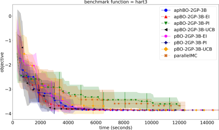
(g) Benchmark by physical wall-clock time.

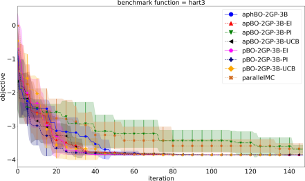
(h) Benchmark by iteration.

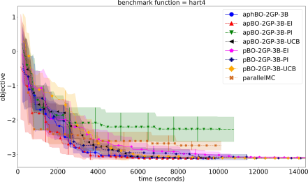
(a) Benchmark by physical wall-clock time.

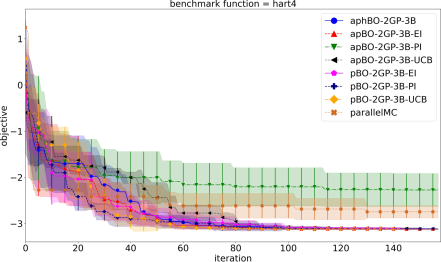
(b) Benchmark by iteration.

(c) Benchmark by physical wall-clock time.

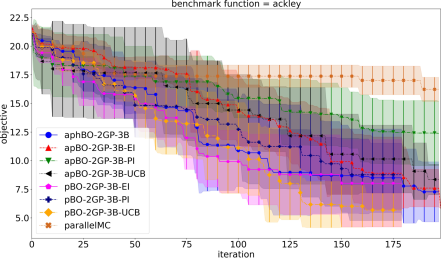
(d) Benchmark by iteration.

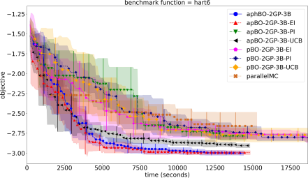
(e) Benchmark by physical wall-clock time.

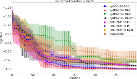
(f) Benchmark by iteration.

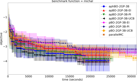
(g) Benchmark by physical wall-clock time.

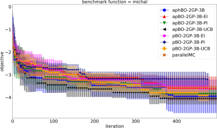
(h) Benchmark by iteration.

Figure 4: Benchmark for michal.

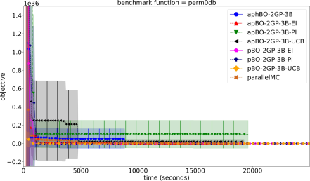
(a) Benchmark by physical wall-clock time.

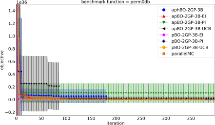
(b) Benchmark by iteration.

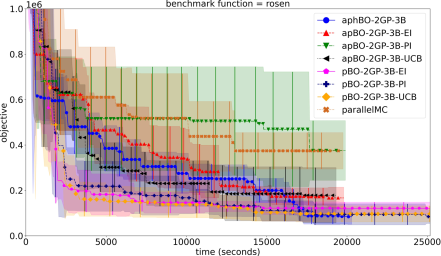
(c) Benchmark by physical wall-clock time.

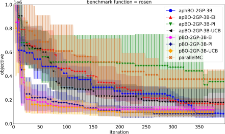
(d) Benchmark by iteration.

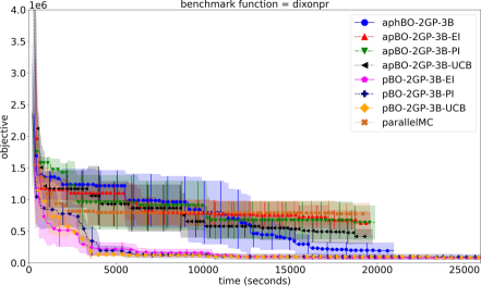
(e) Benchmark by physical wall-clock time.

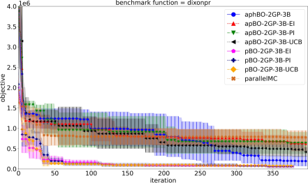
(f) Benchmark by iteration.

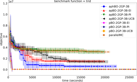
(g) Benchmark by physical wall-clock time.

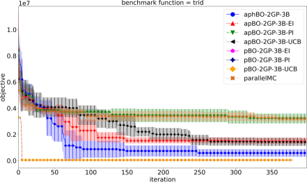
(h) Benchmark by iteration.

Figure 5: Benchmark for trid.

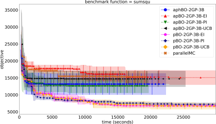
(a) Benchmark by physical wall-clock time.

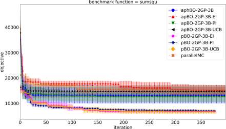
(b) Benchmark by iteration.

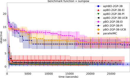
(c) Benchmark by physical wall-clock time.

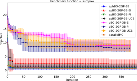
(d) Benchmark by iteration.

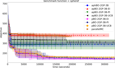
(e) Benchmark by physical wall-clock time.

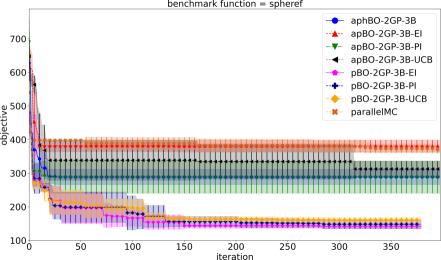
(f) Benchmark by iteration.

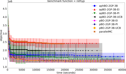
(g) Benchmark by physical wall-clock time.

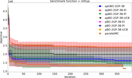
(h) Benchmark by iteration.

Figure 6: Benchmark for rothyp.

Because no constraints are involved in these benchmark functions, the size of the third batch $\displaystyle\mathcal{B}_{\text{exploreClassif}}$ is reduced to zero. Based on the results of Desautels et al. [60], Contal et al. [61], and Tran et al. [2], it has been proved theoretically and shown numerically that parallel BO methods supersede sequential BO methods in term of both convergences in time and in iterations. Therefore, we omit the inclusion of classical BO methods, which are sequential, with different acquisition functions due to its inferiority in numerical performance compared to parallel BO methods. To enhance a fair comparison, we use the same initial points, the same settings for the auxiliary optimizer, as well as the pinging time for checking results periodically, for all methods. It is noted that benchmarking parallel BO methods are very challenging in a shared HPC platform, because the numerical performance may be dependent on the availability of the computational resource.

The results show a significant speedup in low-dimensional problems $\displaystyle(d<10)$, while somewhat on par on high-dimensional problems with the asynchronous parallel feature. Overall, UCB acquisition function is very competitive, compared to both EI and PI acquisition functions. While it is not always the best performer in some benchmark functions, the performance of the proposed aphBO-2GP-3B is stable and nearly optimal across most of the function, which demonstrates its robustness and resiliency. Furthermore, the computational time for asynchronous parallel BO is shorter, while performing on par with the batch-sequential parallel approaches, which makes the former ones more computationally appealing.

5 Engineering example 1: Flip-chip package

In this section, the application of the proposed aphBO-2GP-3B framework to design flip-chip package is demonstrated, where the objective is to minimize the strain energy density, which is an accurate indicator for its fatigue life.

5.1 Thermo-mechanical finite element model

As a possible application of the aphBO-2GP-3B framework, a lidless flip-chip package containing a monolithic silicon die (FCBGA) mounted on a printed circuit board (PCB) with a stiffener ring was considered, such as for a commercial field programmable gate array. The mechanical design space for FCBGAs and PCBs, which represents the dimensions and material choices, was chosen because it is a complex engineering problem with several variables. A parametrized thermo-mechanical FEA model of an FCBGA on PCB was constructed using ANSYS 19.1 using ANSYS Parametric Design Language (APDL) [93].

Table 1: Material properties

Material	CTE (ppm/∘C)	Modulus (GPa)
Silicon	2.6-3.7	169 (x), 130 (y)
SAC305 Solder	22	50
Underfill	30 ($\displaystyle T<T_{g}$), 100 ($\displaystyle T>T_{g}$)	3
Substrate	Variable	30
PCB	Variable	30
Ring Adhesive	120	0.04
Ring	Variable	190
Copper	17	117

Several choices were fixed to facilitate model construction and to represent a realistic design space. For example, only material properties of currently available materials were chosen and interconnect pitches were chosen based on 7nm generation design rules (circa 2020). The variable parameters include die dimensions, substrate dimensions, substrate coefficient of thermal expansion (CTE), ring dimensions, ring CTE, underfill fillet size, and board CTE. The material models are given in Table 1; solder was represented with Anand’s model [94]. A two-dimensional, half symmetry model was chosen to reduce computation time due to the large number of simulations required. While this may lower the numerical accuracy of the model, the relative outputs are not expected to change. The FE model geometry is presented in Figure 7. No validation of the FEA simulation could be performed because no chip was built, however, the authors have previously validated similar models with experimental results [95, 96]. Table 1 presents the material properties used in the FCBGA thermo-mechanical FEA simulation.

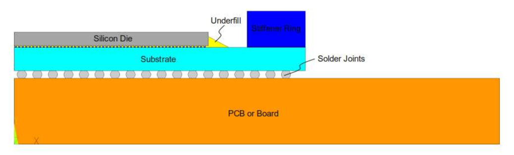
Figure 7: Finite element model geometry.

As an output, after the model is solved, the component warpage at 20^∘C, the component warpage at 200^∘C, and the strain energy density in the outermost solder joint from the third thermal cycle of -40 to 125^∘C [97, 98], are calculated. The component warpage at 20^∘C is a commonly required customer metric, must be below JEDEC specifications [98], as well as component warpage at 200^∘C must be below JEITA [99]. The strain energy density has been identified as an accurate way to predict fatigue life of solder joints during thermal cycling [97]. In this problem, the constraints are imposed that the component warpage at 20^∘C and 200^∘C must be below a 300$\displaystyle\mu$m and 75$\displaystyle\mu$m, respectively. It is noted that the component warpages at different temperatures are only quantifiable if the model converges appropriately. Thus, regression on the constraints is not always possible.

5.2 Optimization results

Table 2 list the design variables and its associated parts, as well as its lower and upper bounds in this case study. The pool of workers used in the optimization is fixed at 16 due to a limited number of licenses. The FEA simulation typically takes about 18-21 minutes on a single processor. For the sake of demonstration, we set the number of processors to one.

Table 2: Design variables for the FCBGA design optimization.

Variable	Design part	Lower bound	Upper bound	Optimal value
$\displaystyle x_{1}$	die	20000	30000	20702
$\displaystyle x_{2}$	die	300	750	320
$\displaystyle x_{3}$	substrate	30000	40000	35539
$\displaystyle x_{4}$	substrate	100	1800	1614
$\displaystyle x_{5}$	substrate	$\displaystyle 10\cdot 10^{-6}$	$\displaystyle 17\cdot 10^{-6}$	$\displaystyle 17\cdot 10^{-6}$
$\displaystyle x_{6}$	stiffener ring	2000	6000	4126
$\displaystyle x_{7}$	stiffener ring	100	2500	1646
$\displaystyle x_{8}$	stiffener ring	$\displaystyle 8\cdot 10^{-6}$	$\displaystyle 25\cdot 10^{-6}$	$\displaystyle 8.94\cdot 10^{-6}$
$\displaystyle x_{9}$	underfill	1.0	3.0	1.52
$\displaystyle x_{10}$	underfill	0.5	1.0	0.804
$\displaystyle x_{11}$	PCB board	$\displaystyle 12.0\cdot 10^{-6}$	$\displaystyle 16.7\cdot 10^{-6}$	$\displaystyle 16.7\cdot 10^{-6}$

Nine initial sampling points are used to initialize the aphBO-2GP-3BO. The interface between the aphBO-2GP-3B framework and the FCBGA application includes a Python and a Shell scripts. A Python script is devised to obtain the output and feasibility of the application, whereas a Shell script is devised to modify the input script for the application and query the script on the HPC platform.

Figure 8 presents the convergence plot of the FCBGA design optimization using the aphBO-2GP-3B framework in 24 hours, where the feasible sampling points are plotted as blue circles, whereas the infeasible sampling points are plotted as red crosses. In total, 1016 simulations are obtained within 24 hours. This is to compare with a traditional BO method, where the same amount of simulations would take 14.11 days, as opposed to 1 day with the aphBO-2GP-3BO framework. The factor of 14.11 in time difference is attributed to a number of factors, mainly the waiting time when submitting a job on the shared HPC. This issue of waiting time in the HPC queue is very common in academic or government environment settings, but not in an industrial setting. It is also shown in Figure 8 that the FCBGA application is highly constraint, where most of the input space is infeasible. Thus, the effectiveness of the GP binary classifier in the aphBO-2GP-3BO is demonstrated.

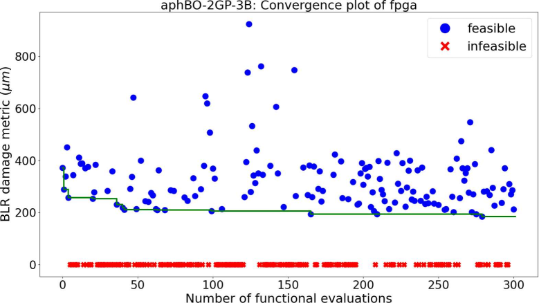
Figure 8: Convergence plot of the aphBO-2GP-3B framework for the FCBGA design optimization application.

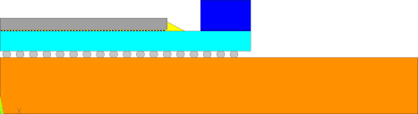
(a) Original design in $\displaystyle xy$-plane.

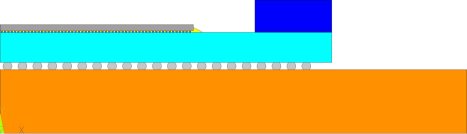
(b) Optimal design in $\displaystyle xy$-plane.

Figure 9: Comparison between original design (Figure 9(a)) and optimal design (Figure 9(b)) of flip-chip package.

The performance of the optimal package is evaluated at different temperatures to further examine its robustness for a range of temperature, from -40^∘C to 200^∘C. Figures 10(a), 10(b), and 10(c) show the contours of the predicted component warpage at the temperatures of -40^∘C, 20^∘C, and 200^∘C, respectively.

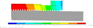
(a) Component warpage evaluation at -40^∘C.

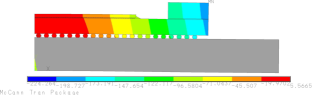
(b) Component warpage evaluation at 20^∘C.

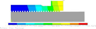
(c) Component warpage evaluation at 200^∘C.

Figure 10: Warpage contour of the optimal flip-chip package at different temperatures, -40^∘C, 20^∘C, and 200^∘C.

Figure 9(a) shows the original design of the flip-chip package, whereas Figure 9(b) shows the optimal design of the flip-chip package as the result of applying the aphBO-2GP-3BO framework. The aphBO-2GP-3BO optimized solution is shown in Table 2. The values are relatively close to the designs used in the microelectronics packaging industry, indicating that the commercial package design is relatively well optimized and validating the aphBO-2GP-3BO result. Specifically, the die is relatively thin and small and the substrate is thick to minimize the component warpage. The substrate CTE is close to the PCB board CTE to improve board level reliability. The substrate size may increase with little impact to the constraints monitored here. The underfill fillet size and ring dimensions are close to industry designs. The stiffener ring CTE is the one notable excursion from industry design, although industry is constrained by actual material selection, which includes cost, manufacturability, and availability, which are not reflected in aphBO-2GP-3BO’s constraints. The BLR damage metric, which is the objective of this case study, is reduced from 372 $\displaystyle\mu m$ to 185 $\displaystyle\mu m$, representing 50.27% improvement.

6 Engineering example 2: 3D CFD slurry pump casing design optimization

In this section, we demonstrate the aphBO-2GP-3B framework using a 3D multiphase CFD simulation. An in-house multiphase CFD wear code is utilized to predict the wear rate of different slurry pump casing. In order to optimize the slurry pump casing performance, the predicted maximum wear rate of the casing is considered as the objective function.

6.1 3D CFD casing wear model

The CFD simulation assumes a constant particle size (or mono-size) and thus the number of species in the particle size distribution is simplified to one. A 14-dimensional input $\displaystyle\bm{x}$ is formed for each CFD simulation to model the geometry of the slurry pump casing. The optimization procedure is carried out for pump assembly Z0534, at the input operating conditions of $\displaystyle Q=89637.900$ gpm, $\displaystyle H=50$ m, $\displaystyle n=849.000$ RPM, $\displaystyle\eta=82.400$, $\displaystyle d_{50}=300\mu$m, $\displaystyle d_{85}=690\mu$m, $\displaystyle d_{\text{eff}}=495\mu$m, $\displaystyle C_{v}=20\%$, and %BEPQ = 99.6%, where $\displaystyle Q$ is the volumetric flow rate, $\displaystyle N$ is the impeller angular speed, $\displaystyle\eta$ is the hydraulic efficiency. $\displaystyle d_{50}$, $\displaystyle d_{85}$ are the 50th and 85th percentile of the particle size distribution. $\displaystyle d_{\text{eff}}=495\mu$m is the effective particle size, which is calculated as the average of the $\displaystyle d_{50}$ and $\displaystyle d_{85}$ and used as an input for mono-size species in the CFD simulation. $\displaystyle\%BEPQ$ is the percentage of best efficiency point flow rate. The design impeller vane diameter is 1.7018 m, the shroud diameter is 1.7780 m, the suction diameter is 0.6604 m, and the discharge diameter is 0.6096 m. The pump specific speed $\displaystyle N_{s}$ in US units in 1425.6.

6.2 CFD casing wear model

The multiphase CFD casing wear model to predict erosive wear in the slurry centrifugal casing is the co-authors’ previous work [100, 101]. A short summary of the simulation is provided for the sake of completeness. The computational domain of the 3D CFD casing wear model is presented in Figure 11(a). Using volume and time averaged governing equations, the continuity and momentum equations of the mixture and different solids species is derived based on an Eulerian-Eulerian framework. The particle size distribution can be discretized into finitely many subclasses, where each of them is treated using the Eulerian approach described above. Figure 11(b) presents three sections of the casing inlet. Different inlet velocity boundary conditions are applied on the region AA’, BC, and B’C’. Based on the head $\displaystyle H$ and flow rate, $\displaystyle Q$, of the slurry pump, the radial and tangential velocities are imposed independently. The regions AB and A’B’ are treated as impermeable walls, where Spalding wall functions [102] are applied. Similar to the CFD impeller wear model [103], in CFD casing wear model, the Spalart-Allmaras turbulence model [104] is used. The set of nonlinear governing equations in the finite element problem are solved iteratively until a steady numerical solution with a tolerable residual level is obtained. Based on the steady-state CFD solutions, the constitutive model for wear prediction is applied with the empirically determined wear coefficients [100, 101] to predict the sliding wear and impact wear as a function of concentration, solids density, velocity magnitude, tangential velocity, shear stress, impingement angle, and the particle size. The total wear is simply the sum of the calculated sliding wear and impact wear.

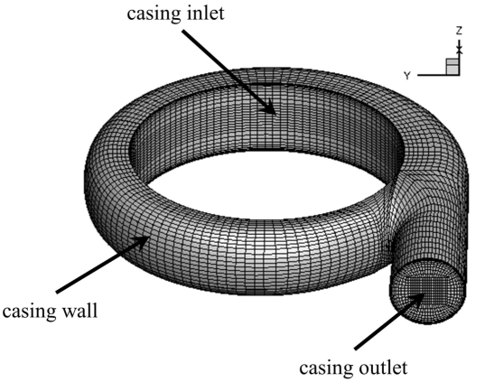
(a) 3D pump casing with mesh and its boundary conditions.

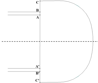
(b) Sections of casing inlet.

Figure 11: Mesh and boundary condition for the 3D CFD casing pump design optimization.

6.3 Optimization results

In this example, the aphBO-2GP-3B framework is combined with the 3D multiphase CFD simulation described above on a Intel Xeon Silver 4110 x2 @2.10GHz machine with 16 cores, 32 threads, 256GB of memory where Ubuntu 18.04 LTS is the operating system.

Two Python scripts are devised to write the input script and read the output for the CFD application. The computational runtime varies between 6.8 to 13.83 hours, depending on the convergence of the design. The optimization case study is performed for approximately 168 hours, which is equivalent to approximately 1176 CPU hours. The batch sizes are set at (5,3,1) for $\displaystyle(\mathcal{B}_{\text{acquisition}},\mathcal{B}_{\text{explore}},\mathcal{B}_{\text{exploreClassif}})$, respectively.

Figure 12 shows the convergence plot of the aphBO-2GP-3B framework for the CFD application, where the first functional evaluation is the original design. The maximum wear rate in the original design is calculated as 116.7958$\displaystyle\mu m/hr$, whereas in the optimal design, the maximum wear rate is calculated as 64.0584$\displaystyle\mu m/hr$, showing an improvement of 45.915% reduction in wear.

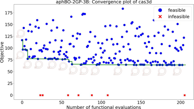
Figure 12: Convergence plot of the aphBO-2GP-3B framework for the 3D CFD slurry pump casing design optimization application with evolutionary designs.

(a) Original design.

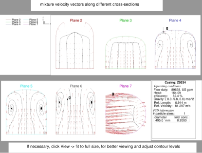
(b) Optimal design.

(c) Original design.

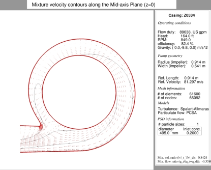
(d) Optimal design.

Figure 13: Comparison of mixture velocity.

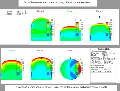
(a) Original design.

(b) Optimal design.

(c) Original design.

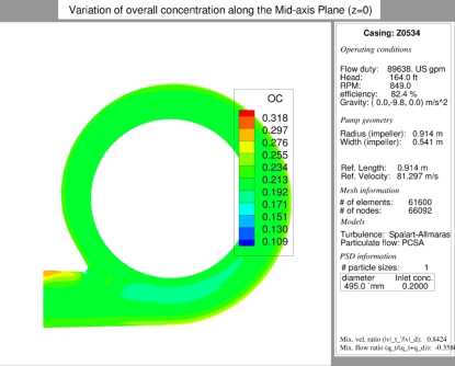
(d) Optimal design.

Figure 14: Comparison of overall concentration.

(a) Original design.

(b) Optimal design.

(c) Original design.

(d) Optimal design.

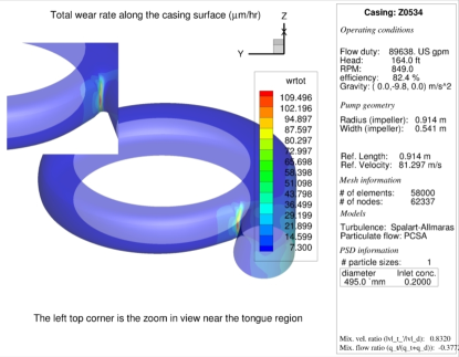
(e) Original design.

(f) Optimal design.

Figure 15: Comparison of wear.

Figure 13 compares the velocity fields in original and optimal design, where Figure 13(a) and Figure 13(b) show the mixture velocity fields of the original and optimal designs, respectively, at different cross sections. It is observed that secondary flows significantly increase in the optimal design, which may help reducing the wear rate on the casing wall. The magnitude of the velocity fields are comparable to each other. Figure 13(c) and Figure 13(d) show the mixture velocity contour in the symmetric midplane of the slurry pump casing. Even though the geometry models are slightly different, the velocity fields in the midplane are nearly identical to each other, in terms of both direction and magnitude.

Figure 14 compares the concentration fields between the original and optimal designs. Figure 14(a) and Figure 14(b) show the overall concentration fields in original and optimal designs, respectively. The concentration field of the optimal design is slightly higher than that of the original design. Differences in geometry models between the original and optimal designs at various cross sections are shown. The height of the cross sections are significantly increased, whereas the width of the cross sections are slightly decreased. The pattern of the concentration fields are also similar between the original and optimal designs.

Figure 15 compares the wear, which are the main concern in this case study, between the original and optimal designs. Figure 15(a) and Figure 15(b) show the impact wear in the casing between the original and optimal designs, respectively, where the optimal design shows significant reduction in terms of magnitude. Near the tongue region of the casing, the hot spot area slightly increases. Figure 15(c) and Figure 15(d) show the sliding wear between original and optimal designs, respectively. Again, significant reduction in sliding wear is observed, which subsequently lead to a significant reduction in total wear, shown in Figure 15(e) and Figure 15(f) for original and optimal designs, respectively. For a comprehensive comparison between original and optimal casing designs, we refer the readers to B.

7 Discussion

One important feature of asynchronous BO is that the users can be more patient with the cases that are difficult to converge (i.e. converge after a long time), particularly for applications where the computational runtime varies widely. The main reason is that the HPC budget is used efficiently in the aphBO-2GP-3B framework, thus increasing the aggressiveness by reducing the waiting time will not improve the efficiency much. Compared to other synchronous batch-sequential parallel approaches, in which the whole batch might halt due to one ill-conditioned simulation, the asynchronous parallel feature relaxes the constraints of thresholding the computational time for the simulation. However, it is recommended to choose the cutoff computational time appropriately depending on the application.

Multiple acquisition functions are considered using the GP-Hedge [3] approach, resulting in further increases in computational efficiency. Compared to our previous pBO-2GP-3B approach, the aphBO-2GP-3B framework is improved in terms of computational efficiency. This is achieved by firstly reducing the waiting time of other computational workers, and secondly by considering multiple acquisition functions and promoting the one which corresponds to better performance.

One of the main drawbacks of BO is the scalability of the surrogate GP model, which prevents the traditional BO method from observing more than $\displaystyle 10^{4}$ sample points. However, this issue is usually not critical for applications with high-fidelity expensive simulations. Because the computational time for one simulation is already computationally substantial, $\displaystyle 10^{4}$ simulations would be significantly computationally expensive. However, scalable GP methods exist to cope with its scalability drawback. For example, a few well-known methods are subset of data [11], the subset of regressor, the deterministic training conditional, and the partially and fully independent training conditions approximations [105, 106].

The aphBO-2GP-3B framework can also be extended to solve equality constraints, for example, by adopting the augmented Lagrangian approach, as well as optimization under uncertainty where noisy evaluation is common. Such problems are more challenging due to its noisy nature. For noisy problems, one can consider Letham et al. [107] approach or stochastic kriging [108] to further improve the current framework.

In this paper, the batch sizes are assumed to be constant and are user-defined parameters. More adaptive approaches can be used to further improve the computational efficiency of the proposed aphBO-2GP-3B framework, where more exploration is promoted at the beginning of the optimization process, and more exploitation is promoted later on. This can be achieved by generalizing the GP-Hedge scheme to include more acquisition functions. However, the inner parameters of GP-Hedge may need to be calibrated again, as the objectives of batches differ greatly.

One may can also consider to integrate a dynamic resource allocation on the top of the current aphBO-2GP-3B framework to reduce the computational time. In HPC settings, the average waiting time and the number of available processors are insightful information that can be used to change the batch sizes adaptively.

We propose to learn the feasible and infeasible regions adaptively by borrowing different binary classifiers in machine learning context. There is no restriction in choosing the binary probabilistic classifier. However, it is noted that the numerical performance of aphBO-2GP-3BO depends on the performance of the binary classifier, as the probability is used to locate the next sampling point. Also, the third batch in the aphBO-2GP-3B framework is designed to force the classifier to learn in its most uncertain regions. This feature is only available for a few binary classifier, such as GP, where the uncertainty can be quantified.

However, the current aphBO-2GP-3B framework does not rigorously solve the dynamic resource allocation problem on the HPC platform, where the computational resource is typically shared where computational constraints are also involved. This opens up the opportunity for further research in the future to consider the BO method in the context of online dynamic HPC resources.

8 Conclusion

In this paper, we present an asynchronous parallel BO method that supports known and unknown constraints in the context of HPC platform. We show that the proposed aphBO-2GP-3B framework can be easily applied for computationally expensive high-fidelity applications in industrial settings. The aphBO-2GP-3B framework is constructed based on two GPs associated with three distinct batches. The first GP corresponds to the objective function, as in the traditional BO method. The first GP is associated with the first and second batch, where the first batch aims to optimize and the second batch aims to explore most uncertain regions. The second GP corresponds to the binary classifier, where uncertainty is measured, and the GP classifier is forced to learn according to the third batch. The hallucination module, which is similar to the kriging heuristic liar approach, allows to construct the GP at the sampling locations where observations are not made yet. This allows the BO framework to move forward and parallelize the optimization, while temporarily disintegrating with the application and waiting for its feedback on completion later on.

The aphBO-2GP-3B approach is demonstrated using two industrial applications. The first application is concerned with the design of flip-chip package, where a thermo-mechanical FEA model is used to predict the fatigue life. The second application is concerned with the design of slurry pump casing, where a 3D multiphase CFD simulation is used to predict the wear rate of the pump casing. It has been shown the aphBO-2GP-3B can highly parallelize across different multi-core HPCs, thus demonstrating the effectiveness of the proposed framework.

Appendix A Numerical benchmark results

In this appendix, we provide more benchmark results for the proposed asynchronous parallel method, aphBO-2GP-3B, particularly on the portfolio of the acquisition function sampled.

• eggholder (2d): batch size = (2,2,0): max iteration = 80

• three-hump camel (2d): batch size = (2,2,0): max iteration = 80

• six-hump camel (2d): batch size = (3,1,0): max iteration = 80

• hartmann (3d): batch size = (3,3,0): max iteration = 150

• hartmann (4d): batch size = (4,4,0): max iteration = 160

• ackley (free d) (5d): batch size = (6,4,0): max iteration = 200

• hartmann (6d): batch size = (5,5,0): max iteration = 300

• michalewicz (free d) (10d): batch size = (5,5,0): max iteration = 400

• perm0db (free d) (80d): batch size = (6,4,0): max iteration = 400

• rosenbrock (free d) (20d): batch size = (6,4,0): max iteration = 400

• dixon-price (free d) (25d): batch size = (7,7,0): max iteration = 480

• trid (free d) (30d): batch size = (6,4,0): max iteration = 400

• sumsqu (free d) (40d): batch size = (6,4,0): max iteration = 400

• sumpow (free d) (50d): batch size = (6,4,0): max iteration = 400

• spheref (free d) (60d): batch size = (6,4,0): max iteration = 400

• rothyp (free d) (70d): batch size = (6,4,0): max iteration = 400

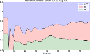
(a) egg: acquisition portfolio.

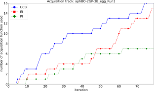
(b) egg: number of acquisition functions.

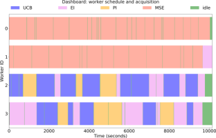
(c) egg: scheduler dashboard.

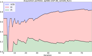
(d) camel6: acquisition portfolio.

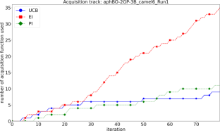
(e) camel6: number of acquisition functions.

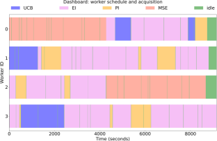
(f) camel6: scheduler dashboard.

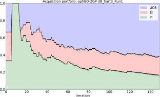
(g) hart3: acquisition portfolio.

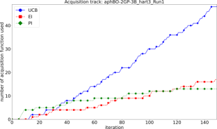
(h) hart3: number of acquisition functions.

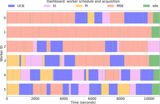
(i) hart3: scheduler dashboard.

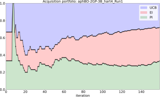
(j) hart4: acquisition portfolio.

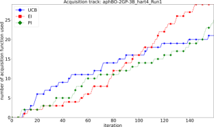
(k) hart4: number of acquisition functions.

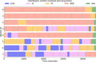
(l) hart4: scheduler dashboard.

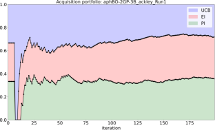
(m) ackley: acquisition portfolio.

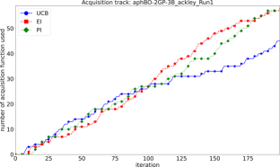
(n) ackley: number of acquisition functions.

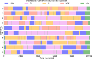
(o) ackley: scheduler dashboard.

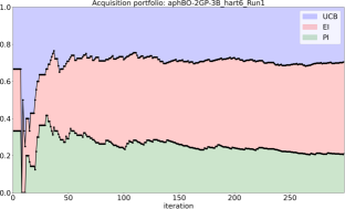
(a) hart6: acquisition portfolio.

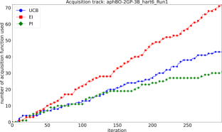
(b) hart6: number of acquisition functions.

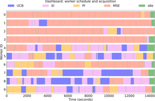
(c) hart6: scheduler dashboard.

(d) michal: acquisition portfolio.

(e) michal: number of acquisition functions.

(f) michal: scheduler dashboard.

(g) perm0db: acquisition portfolio.

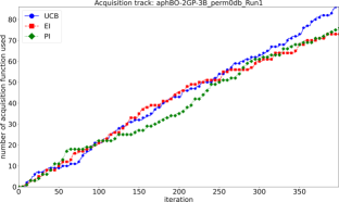
(h) perm0db: number of acquisition functions.

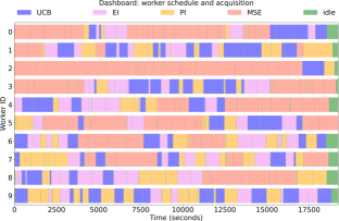
(i) perm0db: scheduler dashboard.

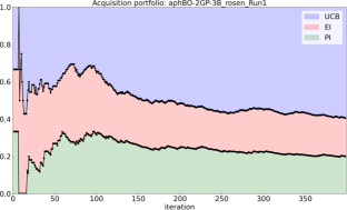
(j) rosen: acquisition portfolio.

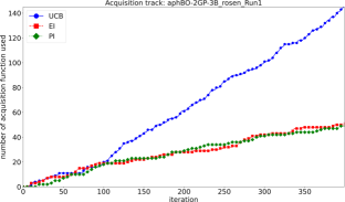
(k) rosen: number of acquisition functions.

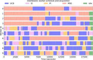
(l) rosen: scheduler dashboard.

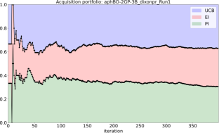
(m) dixonpr: acquisition portfolio.

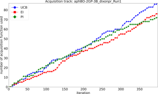
(n) dixonpr: number of acquisition functions.

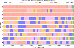
(o) dixonpr: scheduler dashboard.

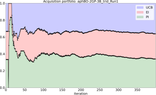
(a) trid: acquisition portfolio.

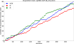
(b) trid: number of acquisition functions.

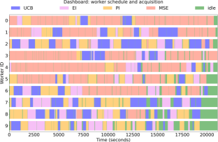
(c) trid: scheduler dashboard.

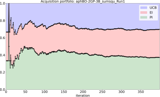
(d) sumsqu: acquisition portfolio.

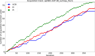
(e) sumsqu: number of acquisition functions.

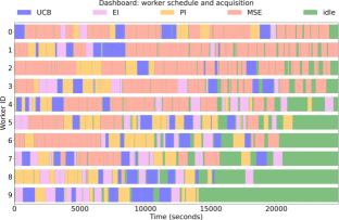
(f) sumsqu: scheduler dashboard.

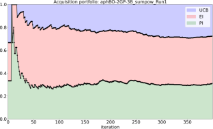
(g) sumpow: acquisition portfolio.

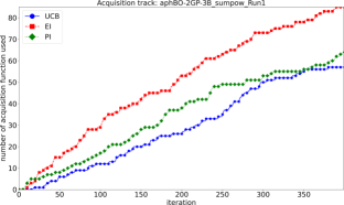
(h) sumpow: number of acquisition functions.

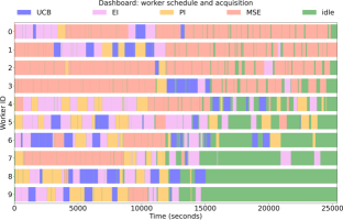
(i) sumpow: scheduler dashboard.

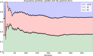
(j) spheref: acquisition portfolio.

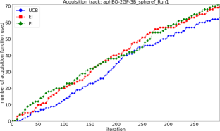
(k) spheref: number of acquisition functions.

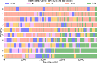
(l) spheref: scheduler dashboard.

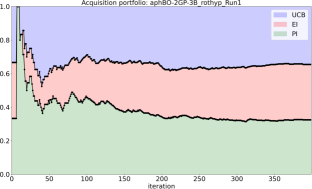
(m) rothyp: acquisition portfolio.

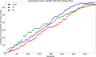
(n) rothyp: number of acquisition functions.

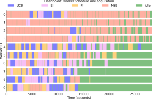
(o) rothyp: scheduler dashboard.

Appendix B CFD results

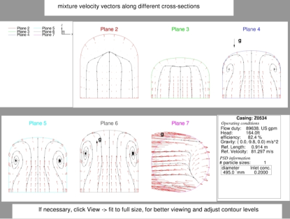
(a) Original design.

(b) Optimal design.

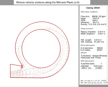
(c) Original design.

(d) Optimal design.

Figure 19: Comparison of mixture velocity.

(a) Original design.

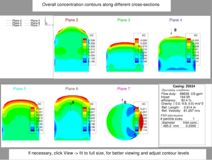
(b) Optimal design.

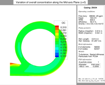
(c) Original design.

(d) Optimal design.

Figure 20: Comparison of overall concentration.

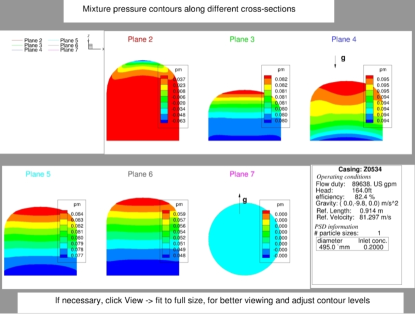
(a) Original design.

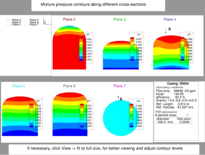
(b) Optimal design.

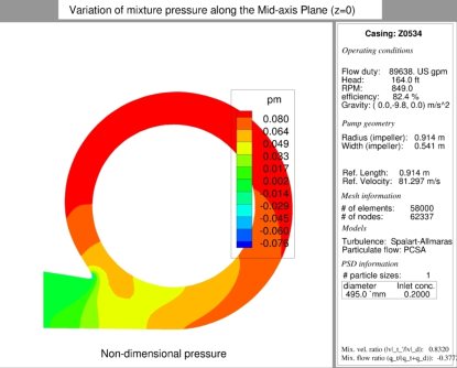
(c) Original design.

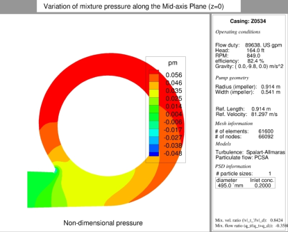
(d) Optimal design.

Figure 21: Comparison of pressure mixture.

(a) Original design.

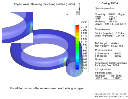
(b) Optimal design.

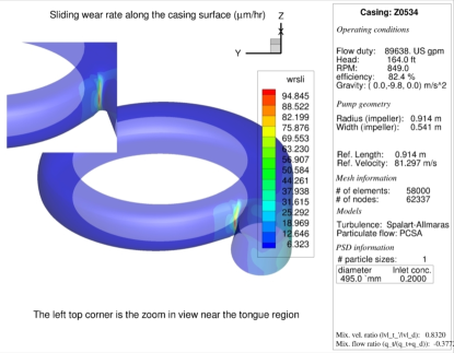
(c) Original design.

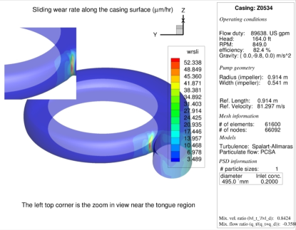
(d) Optimal design.

(e) Original design.

(f) Optimal design.

Figure 22: Comparison of wear in 3D.

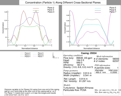
(a) Original design.

(b) Optimal design.

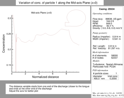
(c) Original design.

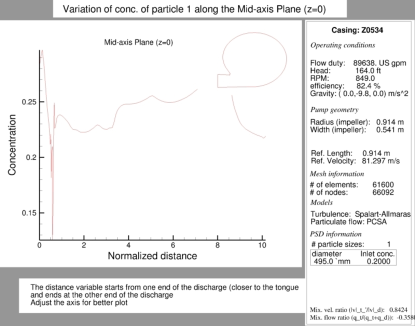
(d) Optimal design.

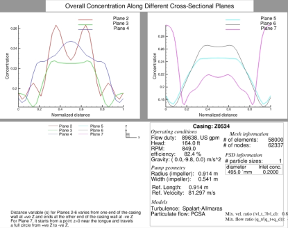
(e) Original design.

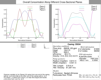
(f) Optimal design.

Figure 23: Comparison of concentration.

(a) Original design.

(b) Optimal design.

(c) Original design.

(d) Optimal design.

Figure 24: Comparison of impact angle.

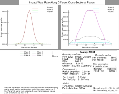
(a) Original design.

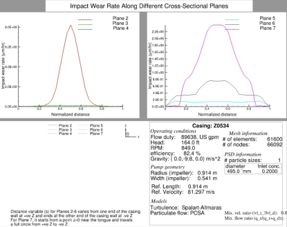
(b) Optimal design.

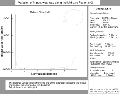
(c) Original design.

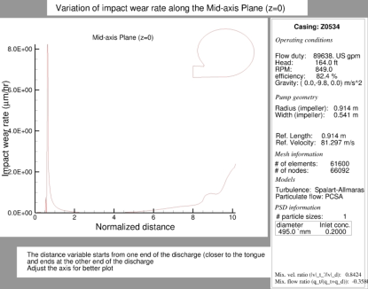
(d) Optimal design.

Figure 25: Comparison of impact wear.

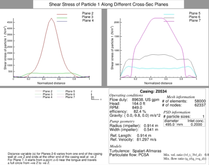
(a) Original design.

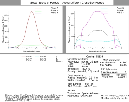
(b) Optimal design.

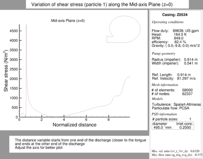
(c) Original design.

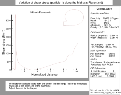
(d) Optimal design.

Figure 26: Comparison of shear stress.

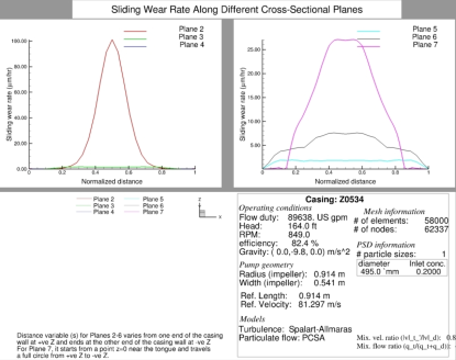
(a) Original design.

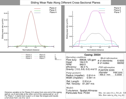
(b) Optimal design.

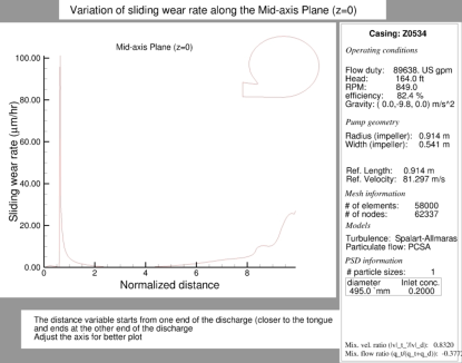
(c) Original design.

(d) Optimal design.

Figure 27: Comparison of sliding wear.

(a) Original design.

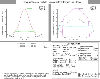
(b) Optimal design.

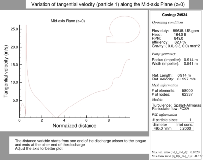
(c) Original design.

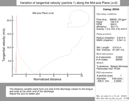
(d) Optimal design.

Figure 28: Comparison of tangential velocity.

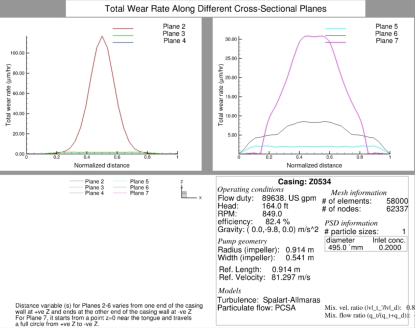
(a) Original design.

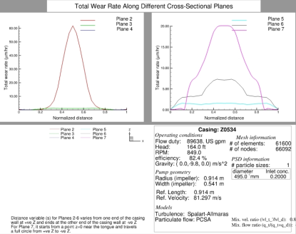
(b) Optimal design.

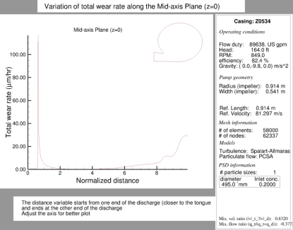
(c) Original design.

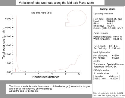
(d) Optimal design.

Figure 29: Comparison of total wear.

(a) Original design.

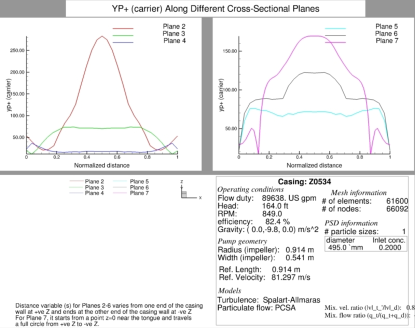
(b) Optimal design.

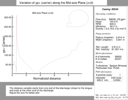
(c) Original design.

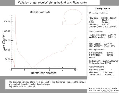
(d) Optimal design.

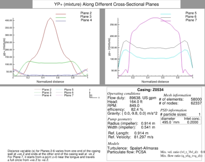
(e) Original design.

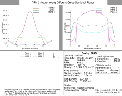
(f) Optimal design.

Figure 30: Comparison of $\displaystyle y^{+}$ value.

(a) Original design.

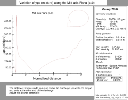
(b) Optimal design.

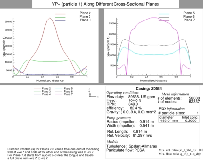
(c) Original design.

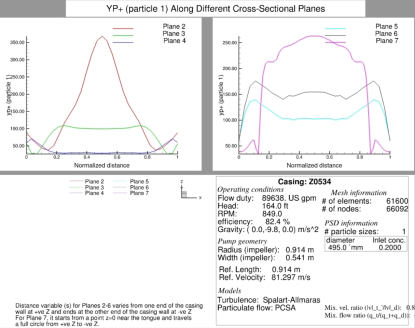
(d) Optimal design.

(e) Original design.

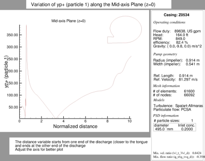
(f) Optimal design.

Figure 31: Comparison of $\displaystyle y^{+}$ value.

References

- [1] D. R. Jones, M. Schonlau, W. J. Welch, Efficient global optimization of expensive black-box functions, Journal of Global Optimization 13 (4) (1998) 455–492.
- [2] A. Tran, J. Sun, J. M. Furlan, K. V. Pagalthivarthi, R. J. Visintainer, Y. Wang, pBO-2GP-3B: A batch parallel known/unknown constrained Bayesian optimization with feasibility classification and its applications in computational fluid dynamics, Computer Methods in Applied Mechanics and Engineering 347 (2019) 827–852.
- [3] M. Hoffman, E. Brochu, N. de Freitas, Portfolio allocation for bayesian optimization, in: Proceedings of the Twenty-Seventh Conference on Uncertainty in Artificial Intelligence, UAI’11, AUAI Press, Arlington, Virginia, USA, 2011, pp. 327–336.
- [4] E. Brochu, V. M. Cora, N. de Freitas, A tutorial on Bayesian optimization of expensive cost functions, with application to active user modeling and hierarchical reinforcement learning, arXiv preprint arXiv:1012.2599 (2010).
- [5] B. Shahriari, K. Swersky, Z. Wang, R. P. Adams, N. de Freitas, Taking the human out of the loop: A review of Bayesian optimization, Proceedings of the IEEE 104 (1) (2016) 148–175.
- [6] P. I. Frazier, A tutorial on Bayesian optimization, arXiv preprint arXiv:1807.02811 (2018).
- [7] A. Tran, T. Wildey, S. McCann, sMF-BO-2CoGP: A sequential multi-fidelity constrained Bayesian optimization for design applications, Journal of Computing and Information Science in Engineering 20 (3) (2020) 1–15.
- [8] A. Tran, Y. Wang, J. Furlan, K. V. Pagalthivarthi, M. Garman, A. Cutright, R. J. Visintainer, WearGP: A UQ/ML wear prediction framework for slurry pump impellers and casings, in: ASME 2020 Fluids Engineering Division Summer Meeting, American Society of Mechanical Engineers, 2020.
- [9] A. Tran, T. Wildey, S. McCann, sBF-BO-2CoGP: A sequential bi-fidelity constrained Bayesian optimization for design applications, in: Proceedings of the ASME 2019 IDETC/CIE, Vol. Volume 1: 39th Computers and Information in Engineering Conference of International Design Engineering Technical Conferences and Computers and Information in Engineering Conference, American Society of Mechanical Engineers, 2019, v001T02A073.
- [10] A. Tran, M. Tran, Y. Wang, Constrained mixed-integer Gaussian mixture Bayesian optimization and its applications in designing fractal and auxetic metamaterials, Structural and Multidisciplinary Optimization (2019) 1–24.
- [11] A. Tran, L. He, Y. Wang, An efficient first-principles saddle point searching method based on distributed kriging metamodels, ASCE-ASME Journal of Risk and Uncertainty in Engineering Systems, Part B: Mechanical Engineering 4 (1) (2018) 011006.
- [12] A. Tran, J. M. Furlan, K. V. Pagalthivarthi, R. J. Visintainer, T. Wildey, Y. Wang, WearGP: A computationally efficient machine learning framework for local erosive wear predictions via nodal Gaussian processes, Wear 422 (2019) 9–26.
- [13] C. E. Rasmussen, Gaussian processes in machine learning, MIT Press, 2006.
- [14] J. Lee, Y. Bahri, R. Novak, S. S. Schoenholz, J. Pennington, J. Sohl-Dickstein, Deep neural networks as Gaussian processes, in: ICLR, 2018.
- [15] A. Garriga-Alonso, C. E. Rasmussen, L. Aitchison, Deep convolutional networks as shallow Gaussian processes, in: ICLR, 2019.
- [16] H. J. Kushner, A new method of locating the maximum point of an arbitrary multipeak curve in the presence of noise, Journal of Basic Engineering 86 (1) (1964) 97–106.
- [17] J. Mockus, On Bayesian methods for seeking the extremum, in: Optimization Techniques IFIP Technical Conference, Springer, 1975, pp. 400–404.
- [18] J. Mockus, The Bayesian approach to global optimization, System Modeling and Optimization (1982) 473–481.
- [19] A. D. Bull, Convergence rates of efficient global optimization algorithms, Journal of Machine Learning Research 12 (Oct) (2011) 2879–2904.
- [20] J. Snoek, H. Larochelle, R. P. Adams, Practical Bayesian optimization of machine learning algorithms, in: Advances in Neural Information Processing Systems, 2012, pp. 2951–2959.
- [21] W. Scott, P. Frazier, W. Powell, The correlated knowledge gradient for simulation optimization of continuous parameters using gaussian process regression, SIAM Journal on Optimization 21 (3) (2011) 996–1026.
- [22] P. Auer, Using confidence bounds for exploitation-exploration trade-offs, Journal of Machine Learning Research 3 (Nov) (2002) 397–422.
- [23] N. Srinivas, A. Krause, S. M. Kakade, M. Seeger, Gaussian process optimization in the bandit setting: No regret and experimental design, arXiv preprint arXiv:0912.3995 (2009).
- [24] N. Srinivas, A. Krause, S. M. Kakade, M. W. Seeger, Information-theoretic regret bounds for Gaussian process optimization in the bandit setting, IEEE Transactions on Information Theory 58 (5) (2012) 3250–3265.
- [25] C. Daniel, M. Viering, J. Metz, O. Kroemer, J. Peters, Active reward learning., in: Robotics: Science and Systems, 2014.
- [26] J. M. Hernández-Lobato, M. W. Hoffman, Z. Ghahramani, Predictive entropy search for efficient global optimization of black-box functions, in: Advances in Neural Information Processing Systems, 2014, pp. 918–926.
- [27] J. M. Hernández-Lobato, M. Gelbart, M. Hoffman, R. Adams, Z. Ghahramani, Predictive entropy search for Bayesian optimization with unknown constraints, in: International Conference on Machine Learning, 2015, pp. 1699–1707.
- [28] D. Hernández-Lobato, J. Hernández-Lobato, A. Shah, R. Adams, Predictive entropy search for multi-objective Bayesian optimization, in: International Conference on Machine Learning, 2016, pp. 1492–1501.
- [29] J. M. Hernández-Lobato, M. A. Gelbart, R. P. Adams, M. W. Hoffman, Z. Ghahramani, A general framework for constrained bayesian optimization using information-based search, Journal of Machine Learning Research (2016).
- [30] P. Hennig, C. J. Schuler, Entropy search for information-efficient global optimization, Journal of Machine Learning Research 13 (Jun) (2012) 1809–1837.
- [31] Z. Wang, S. Jegelka, Max-value entropy search for efficient Bayesian optimization, arXiv preprint arXiv:1703.01968 (2017).
- [32] J. Wilson, F. Hutter, M. Deisenroth, Maximizing acquisition functions for Bayesian optimization, Advances in Neural Information Processing Systems 31 (2018) 9884–9895.
- [33] S. L. Digabel, S. M. Wild, A taxonomy of constraints in simulation-based optimization, arXiv preprint arXiv:1505.07881 (2015).
- [34] J. Parr, A. Keane, A. I. Forrester, C. Holden, Infill sampling criteria for surrogate-based optimization with constraint handling, Engineering Optimization 44 (10) (2012) 1147–1166.
- [35] R. B. Gramacy, H. K. H. Lee, Optimization under unknown constraints, arXiv preprint arXiv:1004.4027 (2010).
- [36] R. B. Gramacy, G. A. Gray, S. Le Digabel, H. K. Lee, P. Ranjan, G. Wells, S. M. Wild, Modeling an augmented Lagrangian for blackbox constrained optimization, Technometrics 58 (1) (2016) 1–11.
- [37] Q. Zhou, Y. Wang, S.-K. Choi, P. Jiang, X. Shao, J. Hu, L. Shu, A robust optimization approach based on multi-fidelity metamodel, Structural and Multidisciplinary Optimization 57 (2) (2018) 775–797.
- [38] M. Schonlau, W. J. Welch, D. R. Jones, Global versus local search in constrained optimization of computer models, Lecture Notes-Monograph Series (1998) 11–25.
- [39] J. R. Gardner, M. J. Kusner, Z. E. Xu, K. Q. Weinberger, J. P. Cunningham, Bayesian optimization with inequality constraints., in: ICML, 2014, pp. 937–945.
- [40] B. Letham, B. Karrer, G. Ottoni, E. Bakshy, et al., Constrained Bayesian optimization with noisy experiments, Bayesian Analysis (2018).
- [41] M. A. Gelbart, J. Snoek, R. P. Adams, Bayesian optimization with unknown constraints, arXiv preprint arXiv:1403.5607 (2014).
- [42] A. Basudhar, C. Dribusch, S. Lacaze, S. Missoum, Constrained efficient global optimization with support vector machines, Structural and Multidisciplinary Optimization 46 (2) (2012) 201–221.
- [43] M. Sacher, R. Duvigneau, O. Le Maître, M. Durand, É. Berrini, F. Hauville, J.-A. Astolfi, A classification approach to efficient global optimization in presence of non-computable domains, Structural and Multidisciplinary Optimization (2018) 1–21.
- [44] H. Lee, R. Gramacy, C. Linkletter, G. Gray, Optimization subject to hidden constraints via statistical emulation, Pacific Journal of Optimization 7 (3) (2011) 467–478.
- [45] M. D. Hill, M. R. Marty, Amdahl’s law in the multicore era, Computer 41 (7) (2008) 33–38.
- [46] D. Ginsbourger, R. Le Riche, L. Carraro, A multi-points criterion for deterministic parallel global optimization based on Gaussian processes (2008).
- [47] D. Ginsbourger, R. Le Riche, L. Carraro, Kriging is well-suited to parallelize optimization, Computational Intelligence in Expensive Optimization Problems 2 (2010) 131–162.
- [48] C. Chevalier, D. Ginsbourger, Fast computation of the multi-points expected improvement with applications in batch selection, in: International Conference on Learning and Intelligent Optimization, Springer, 2013, pp. 59–69.
- [49] O. Roustant, D. Ginsbourger, Y. Deville, DiceKriging, DiceOptim: Two R packages for the analysis of computer experiments by kriging-based metamodelling and optimization, Journal of Statistical Software 51 (1) (2012) 54p.
- [50] S. Marmin, C. Chevalier, D. Ginsbourger, Differentiating the multipoint expected improvement for optimal batch design, in: International Workshop on Machine Learning, Optimization and Big Data, Springer, 2015, pp. 37–48.
- [51] S. Marmin, C. Chevalier, D. Ginsbourger, Efficient batch-sequential Bayesian optimization with moments of truncated Gaussian vectors, arXiv preprint arXiv:1609.02700 (2016).
- [52] J. Wang, S. C. Clark, E. Liu, P. I. Frazier, Parallel Bayesian global optimization of expensive functions, arXiv preprint arXiv:1602.05149 (2016).
- [53] J. Wu, P. Frazier, The parallel knowledge gradient method for batch Bayesian optimization, in: Advances in Neural Information Processing Systems, 2016, pp. 3126–3134.
- [54] P. Frazier, W. Powell, S. Dayanik, The knowledge-gradient policy for correlated normal beliefs, INFORMS journal on Computing 21 (4) (2009) 599–613.
- [55] N. Rontsis, M. A. Osborne, P. J. Goulart, Distributionally robust optimization techniques in batch Bayesian optimization, arXiv preprint arXiv:1707.04191 (2017).
- [56] J. Azimi, A. Fern, X. Z. Fern, Batch Bayesian optimization via simulation matching, in: Advances in Neural Information Processing Systems, 2010, pp. 109–117.
- [57] J. Azimi, A. Fern, X. Zhang-Fern, G. Borradaile, B. Heeringa, Batch active learning via coordinated matching, arXiv preprint arXiv:1206.6458 (2012).
- [58] J. Azimi, A. Jalali, X. Fern, Hybrid batch Bayesian optimization, arXiv preprint arXiv:1202.5597 (2012).
- [59] A. Shah, Z. Ghahramani, Parallel predictive entropy search for batch global optimization of expensive objective functions, in: Advances in Neural Information Processing Systems, 2015, pp. 3330–3338.
- [60] T. Desautels, A. Krause, J. W. Burdick, Parallelizing exploration-exploitation tradeoffs in Gaussian process bandit optimization, The Journal of Machine Learning Research 15 (1) (2014) 3873–3923.
- [61] E. Contal, D. Buffoni, A. Robicquet, N. Vayatis, Parallel Gaussian process optimization with upper confidence bound and pure exploration, in: Joint European Conference on Machine Learning and Knowledge Discovery in Databases, Springer, 2013, pp. 225–240.
- [62] T. Kathuria, A. Deshpande, P. Kohli, Batched Gaussian process bandit optimization via determinantal point processes, in: Advances in Neural Information Processing Systems, 2016, pp. 4206–4214.
- [63] Z. Wang, C. Li, S. Jegelka, P. Kohli, Batched high-dimensional Bayesian optimization via structural kernel learning, arXiv preprint arXiv:1703.01973 (2017).
- [64] E. A. Daxberger, B. K. H. Low, Distributed batch Gaussian process optimization, in: International Conference on Machine Learning, 2017, pp. 951–960.
- [65] J. González, Z. Dai, P. Hennig, N. Lawrence, Batch Bayesian optimization via local penalization, in: Proceedings of the 19th International Conference on Artificial Intelligence and Statistics, 2016, pp. 648–657.
- [66] V. Nguyen, S. Rana, S. K. Gupta, C. Li, S. Venkatesh, Budgeted batch Bayesian optimization, in: Data Mining (ICDM), 2016 IEEE 16th International Conference on, IEEE, 2016, pp. 1107–1112.
- [67] D. Ginsbourger, J. Janusevskis, R. Le Riche, Dealing with asynchronicity in parallel gaussian process based global optimization, in: 4th International Conference of the ERCIM WG on computing & statistics (ERCIM’11), 2011.
- [68] J. Janusevskis, R. Le Riche, D. Ginsbourger, R. Girdziusas, Expected improvements for the asynchronous parallel global optimization of expensive functions: Potentials and challenges, in: Learning and Intelligent Optimization, Springer, 2012, pp. 413–418.
- [69] B. Kamiński, P. Szufel, On parallel policies for ranking and selection problems, Journal of Applied Statistics 45 (9) (2018) 1690–1713.
- [70] H. Kotthaus, J. Richter, A. Lang, J. Thomas, B. Bischl, P. Marwedel, J. Rahnenführer, M. Lang, RAMBO: Resource-aware model-based optimization with scheduling for heterogeneous runtimes and a comparison with asynchronous model-based optimization, in: International Conference on Learning and Intelligent Optimization, Springer, 2017, pp. 180–195.
- [71] K. Kandasamy, A. Krishnamurthy, J. Schneider, B. Poczos, Asynchronous parallel Bayesian optimisation via Thompson sampling, arXiv preprint arXiv:1705.09236 (2017).
- [72] W. R. Thompson, On the likelihood that one unknown probability exceeds another in view of the evidence of two samples, Biometrika 25 (3/4) (1933) 285–294.
- [73] B. S. S. Pokuri, A. Lofquist, C. M. Risko, B. Ganapathysubramanian, PARyOpt: A software for parallel asynchronous remote Bayesian optimization, arXiv preprint arXiv:1809.04668 (2018).
- [74] A. S. Alvi, B. Ru, J. Calliess, S. J. Roberts, M. A. Osborne, Asynchronous batch Bayesian optimisation with improved local penalisation, arXiv preprint arXiv:1901.10452 (2019).
- [75] J. L. Bentley, Multidimensional binary search trees used for associative searching, Communications of the ACM 18 (9) (1975) 509–517.
- [76] T. Hastie, S. Rosset, J. Zhu, H. Zou, Multi-class AdaBoost, Statistics and its Interface 2 (3) (2009) 349–360.
- [77] L. Breiman, Random forests, Machine learning 45 (1) (2001) 5–32.
- [78] M. A. Hearst, S. T. Dumais, E. Osuna, J. Platt, B. Scholkopf, Support vector machines, IEEE Intelligent Systems and their applications 13 (4) (1998) 18–28.
- [79] J. A. Suykens, J. Vandewalle, Least squares support vector machine classifiers, Neural processing letters 9 (3) (1999) 293–300.
- [80] C. E. Rasmussen, Gaussian processes in machine learning, in: Advanced lectures on machine learning, Springer, 2004, pp. 63–71.
- [81] Y. LeCun, Y. Bengio, G. Hinton, Deep learning, nature 521 (7553) (2015) 436.
- [82] B. Shahriari, Z. Wang, M. W. Hoffman, A. Bouchard-Côté, N. de Freitas, An entropy search portfolio for Bayesian optimization, arXiv preprint arXiv:1406.4625 (2014).
- [83] A. De Palma, C. Mendler-Dünner, T. Parnell, A. Anghel, H. Pozidis, Sampling acquisition functions for batch Bayesian optimization, arXiv preprint arXiv:1903.09434 (2019).
- [84] N. Cesa-Bianchi, G. Lugosi, Prediction, learning, and games, Cambridge university press, 2006.
- [85] H. B. Nielsen, S. N. Lophaven, J. Søndergaard, DACE, a MATLAB Kriging toolbox, Vol. 2, Citeseer, 2002.
- [86] D. Gorissen, I. Couckuyt, P. Demeester, T. Dhaene, K. Crombecq, A surrogate modeling and adaptive sampling toolbox for computer based design, The Journal of Machine Learning Research 11 (2010) 2051–2055.
- [87] I. Couckuyt, A. Forrester, D. Gorissen, F. De Turck, T. Dhaene, Blind kriging: Implementation and performance analysis, Advances in Engineering Software 49 (2012) 1–13.
- [88] I. Couckuyt, T. Dhaene, P. Demeester, ooDACE toolbox, A Matlab Kriging toolbox: Getting started, Universiteit Gent (2013) 3–15.
- [89] I. Couckuyt, T. Dhaene, P. Demeester, ooDACE toolbox: a flexible object-oriented Kriging implementation, The Journal of Machine Learning Research 15 (1) (2014) 3183–3186.
- [90] N. Hansen, A. Ostermeier, Completely derandomized self-adaptation in evolution strategies, Evolutionary computation 9 (2) (2001) 159–195.
- [91] N. Hansen, S. D. Müller, P. Koumoutsakos, Reducing the time complexity of the derandomized evolution strategy with covariance matrix adaptation (CMA-ES), Evolutionary computation 11 (1) (2003) 1–18.
- [92] S. Surjanovic, D. Bingham, Virtual library of simulation experiments: test functions and datasets, https://www.sfu.ca/ssurjano/optimization.html.
- [93] S. McCann, S. Kuramochi, H. Yun, V. Sundaram, M. R. Pulugurtha, R. R. Tummala, S. K. Sitaraman, Board-level reliability of 3D through glass via filters during thermal cycling, in: Electronic Components and Technology Conference (ECTC), 2016 IEEE 66th, IEEE, 2016, pp. 1575–1582.
- [94] L. Anand, Constitutive equations for hot-working of metals, International Journal of Plasticity 1 (3) (1985) 213–231.
- [95] S. McCann, Y. Sato, T. Ogawa, R. R. Tummala, S. K. Sitaraman, Use of birefringence to determine redistribution layer stresses to create design guidelines to prevent glass cracking, IEEE Transactions on Device and Materials Reliability 17 (3) (2017) 585–592.
- [96] S. McCann, H. H. Lee, G. Refai-Ahmed, T. Lee, S. Ramalingam, Warpage and reliability challenges for stacked silicon interconnect technology in large packages, in: 2018 IEEE 68th Electronic Components and Technology Conference (ECTC), IEEE, 2018, pp. 2345–2350.
- [97] R. Darveaux, Effect of simulation methodology on solder joint crack growth correlation, in: Electronic Components & Technology Conference, 2000. 2000 Proceedings. 50th, IEEE, 2000, pp. 1048–1058.
- [98] J. Standard, Package warpage measurement of surface-mount integrated circuits at elevated temperature, JESD22-B112 October (2009).
- [99] J. Standard, Measurement methods of package warpage at elevated temperature and maximum permissive warpage, JEITA 7306, March (2007).
- [100] K. V. Pagalthivarthi, R. J. Visintainer, Solid-liquid flow-induced erosion prediction in three-dimensional pump casing, in: ASME 2009 Fluids Engineering Division Summer Meeting, American Society of Mechanical Engineers, 2009, pp. 611–617.
- [101] K. V. Pagalthivarthi, J. M. Furlan, R. J. Visintainer, Finite element prediction of multi-size particulate flow through three-dimensional pump casing, in: ASME/JSME/KSME 2015 Joint Fluids Engineering Conference, American Society of Mechanical Engineers, 2015, pp. V001T31A002–V001T31A002.
- [102] F. White, Viscous Fluid Flow 2nd Edition, McGraw-Hill New York, 1991.
- [103] K. V. Pagalthivarthi, J. M. Furlan, R. J. Visintainer, Wear rate prediction in multi-size particulate flow through impellers, in: ASME 2013 Fluids Engineering Division Summer Meeting, American Society of Mechanical Engineers, 2013.
- [104] P. R. Spalart, S. R. Allmaras, et al., A one equation turbulence model for aerodynamic flows, Recherche Aerospatiale-French Edition (1994) 5–5.
- [105] J. Quiñonero-Candela, C. E. Rasmussen, C. K. Williams, Approximation methods for gaussian process regression, Large-scale kernel machines (2007) 203–224.
- [106] K. Chalupka, C. K. Williams, I. Murray, A framework for evaluating approximation methods for Gaussian process regression, Journal of Machine Learning Research 14 (Feb) (2013) 333–350.
- [107] B. Letham, B. Karrer, G. Ottoni, E. Bakshy, Constrained Bayesian optimization with noisy experiments, arXiv preprint arXiv:1706.07094 (2017).
- [108] B. Ankenman, B. L. Nelson, J. Staum, Stochastic kriging for simulation metamodeling, Operations research 58 (2) (2010) 371–382.