Normal state properties of quantum critical metals at finite temperature

Abstract

We study the effects of finite temperature on normal state properties of a metal near a quantum critical point to an antiferromagnetic or Ising-nematic state. At $T=0$ bosonic and fermionic self-energies are traditionally computed within Eliashberg theory and obey scaling relations with characteristic power-laws. Quantum Monte Carlo (QMC) simulations have shown strong systematic deviations from these predictions, casting doubt on the validity of the theoretical analysis. We extend Eliashberg theory to finite $T$ and argue that for the $T$ range accessible in the QMC simulations, the scaling forms for both fermionic and bosonic self energies are quite different from those at $T=0$. We compare finite $T$ results with QMC data and find good agreement for both systems. This, we argue, resolves the key apparent contradiction between the theory and the QMC simulations.

I Introduction

Electron-boson models Hertz (1976); Millis (1993); Altshuler et al. (1994); Abanov et al. (2003) have long been used to study the behavior of interacting fermions near a metallic quantum critical point (QCP) In these models, a specific channel of the electron-electron interaction is assumed to become critical at a QCP and is represented by a soft collective boson, while all other channels are assumed to be irrelevant to the low energy dynamics near the QCP. Despite their simplicity, such models predict nontrivial correlation effects such as superconductivity and non Fermi-liquid (NFL) behavior in the normal state Altshuler et al. (1994); Abanov et al. (2001, 2003); Metlitski and Sachdev (2010a, b, c); Lederer et al. (2017); Lee (2018); Maslov and Chubukov (2010); Fradkin et al. (2010); Abanov et al. (2001); Wang et al. (2016); Raghu et al. (2015); Metlitski et al. (2015); Lederer et al. (2015). Correlation effects are stronger in two dimensions (2D) than in 3D, consistent with the fact that most systems in which NFL behavior and high-temperature superconductivity have been observed, e.g. Cu- and Fe- based superconductors, are quasi-2D systems Löhneysen et al. (2007); Monthoux et al. (2007); Abanov et al. (2003); Scalapino (2012); Sachdev et al. (2012); Cyr-Choinière et al. (2018); Fernandes et al. (2014); Wang et al. (2015); Wang and Chubukov (2014). Two of the most studied models of metallic quantum criticality are the spin-fermion model (SFM) where the boson describes fluctuations of an antiferromagnetic order parameter, and the Ising-nematic model (INM), where the boson represents an order parameter, which breaks lattice rotational symmetry.

Both the SFM and the INM have been analyzed within the low-energy theory which is termed Eliashberg theory (ET) due to its similarity with the Eliashberg theory of the electron-phonon interaction. The theory assumes that near a QCP, a soft collective boson is a slow mode compared to a dressed fermion. This effectively decouples the fermionic and bosonic degrees of freedom Millis (1992); Abanov et al. (2003); Rech et al. (2006) and makes the problem analytically tractable. In technical terms, in ET the fermionic self-energy $\Sigma(k,\omega)$ is large, but it can be approximated by its value at the Fermi energy $\Sigma(k_{F},\omega)$ and computed perturbatively at one-loop order. Higher-order corrections (commonly termed as vertex corrections) are neglected by the argument that in the processes giving rise to vertex corrections fermions oscillate at frequencies near the bosonic mass shell, which are far away from their own mass shell. In addition, the integration over internal momenta in the one-loop diagram for the fermionic self-energy factorizes into the one transverse to the Fermi surface (FS), which involves only fermionic degrees of freedom, and the one parallel to the FS, involving only bosonic degrees of freedom. In this situation, characteristic momentum deviations from the FS are small, and the integration can be carried out by linearizing the fermionic dispersion near $k_{F}$. By the same argument, the bosonic self-energy is also computed perturbatively, at one-loop order.

The decoupling of the fermions and bosons leads to fermionic self-energy which depends much more strongly on the frequency $\omega$ than on deviation of the momentum from $k_{F}$ transverse to the FS. The magnitude of the $\omega$-dependent self-energy in turn depends on the location of $k_{F}$ on the FS. In the INM, the Eliashberg self-energy scales as $\Sigma(\omega,{\bf k}_{F})\sim\omega^{1/3}_{\mbox{\tiny INM}}\omega^{2/3}$ over the whole FS, except at special points (cold spots), where FL behavior survives. In the SFM, the Eliashberg self-energy scales as $\Sigma(\omega,{\bf k}_{F})\sim\omega_{\mbox{\tiny SFM}}^{1/2}\omega^{1/2}$ at special FS points (hot spots), connected by a momentum vector corresponding to antiferromagnetic order, while everywhere else on the FS the self-energy has a FL form at the lowest frequencies and crosses over to $\omega^{1/2}$ behavior at a characteristic frequency proportional to the deviation from a hot spot. The $\omega_{\mbox{\tiny SFM}}$ and $\omega_{\mbox{\tiny INM}}$ are characteristic frequencies, which we discuss below. Both remain finite at a QCP.

The validity of the ET in the case when a soft boson is a collective mode of fermions is a more tricky issue than for the original Eliashberg theory of superconductivity, where the boson is an independent degree of freedom (a phonon). For that theory, the applicability condition is the smallness of the ratio $\omega_{0}/E_{F}\sim v_{0}/v_{F}$, where $\omega_{0}$ is the characteristic phonon frequency and $v_{0}$ is the corresponding boson velocity (the dressed Debye frequency and sound velocity for an acoustic phonon) and $E_{F}$ is the Fermi energy (this allows one to factorize the momentum integration), and the smallness of the ratio $\alpha^{2}/(\omega_{0}E_{F})$, where $\alpha$ is the effective fermion-boson coupling (this allows one to neglect vertex corrections). The last condition is not satisfied when $\omega_{0}$ vanishes, but for large enough $E_{F}$ it holds in a wide range of $\omega_{0}$ (Ref. Chubukov et al. (2020)). When the boson is a collective mode in the spin or charge channel, its bare velocity is of order of $v_{F}$, so at the bare level the ET is inapplicable. However, in both the SFM and INM a dressed collective boson is Landau overdamped due to decay into particle-hole pairs. This opens up a possibility that at low energies a dressed boson becomes slow compared to a dressed fermion, i.e., ET becomes applicable as an effective theory, which describes dressed bosons and fermions at low energies. For the INM, the Landau-overdamped boson is slow compared to dressed fermions by $(\omega/\omega_{{\mbox{\tiny INM}}})^{1/3}$ (Refs. Altshuler et al., 1994; Rech et al., 2006; Lee, 2009), which justifies factorization of momentum integration leading to $\omega^{2/3}$ scaling at a QCP. Vertex corrections diverge at a QCP, when calculated with free fermions, but remain finite within the effective ET. The lowest-order vertex correction is of order one, but can be made parametrically small if one extends the theory to $N\gg 1$ fermionic flavors Altshuler et al. (1994); Rech et al. (2006). two loops, however, there are unavoidable logarithmical singularities for both $\Sigma({\bf k}_{F},\omega)$ and $\Sigma({\bf k},0)$ (Refs. Metlitski and Sachdev, 2010a; S-S. Lee, ). These logarithms come from special “planar diagrams”, which describe hidden 1D processes with momentum transverse either $0$ or $2k_{F}$ (Ref. Lee, 2009). Logarithmical corrections were also reported for a bosonic propagator in 5-loop calculations Holder and Metzner (2015a, b). These logarithms are not accounted for in the effective ET. For the SFM, the velocities of dressed fermions and bosons are comparable, i.e., corrections to $\Sigma_{SFM}(\omega)=\omega^{1/2}\omega^{1/2}_{SFM}$ are of order one. This can be cured by extending the theory to $N\gg 1$ fermionic flavors, in which case the corrections to factorization are small in $1/N$. The $k-$dependent self-energy and vertex are also small in $1/N$. However, just like in the INM, there are logarithmical corrections to the effective ET. Moreover, in the SFM, logarithms appear already in one-loop $\Sigma(k)$ and vertex corrections Abanov et al. (2003); Metlitski and Sachdev (2010b); Lee (2018).

This analysis shows that for both models the effective ET becomes invalid below some characteristic frequency, at which logarithmic corrections become of order one. However, for the breakdown of ET to occur, this frequency must be larger than superconducting $T_{c}$, otherwise the logarithmic singularities will be cut off by the opening of a gap due to superconductivity. In the SFM, $T_{c}$ generally of order $\omega_{\mbox{\tiny SFM}}$, and in the INM $T_{c}\sim\omega_{\mbox{\tiny INM}}$ (Refs. Abanov et al., 2001, 2003; Metlitski et al., 2015; Wang and Chubukov, 2013; Bonesteel et al., 1996). At such frequencies, some calculations show Chubukov et al. (1997) that corrections to ET may be small numerically, in which case the effective ET should remain valid, at least qualitatively.

The validity of the effective ET at a QCP has been recently tested in a series of sign-free quantum Monte Carlo (QMC) simulations of both the SFM and INM. Schattner et al. (2016a); Lederer et al. (2017); Gerlach et al. (2017); Schattner et al. (2016b); Wang et al. (2017); Liu et al. (2018); Xu et al. (2017a, b). Such simulations are numerical experiments that test effective models of quantum-critical metals Xu et al. (2017b, 2019); Berg et al. (2019). QMC data were taken at temperatures above $T_{c}$, where ET is expected to work. Analysis of the QMC data revealed that some properties, most strikingly the superconducting $T_{c}$ of the SFM, agreed well with predictions of ETWang et al. (2017). However, other properties showed systematic deviations from ET. In particular, for both SFM and INM, fermionic self-energies in the normal state, extracted from QMC, do not show the power-law forms, expected from the theory, and appear to saturate at a finite value even at the smallest fermionic Matsubara frequency $\omega=\pi T$. In addition, the bosonic self-energy in the INM does not show the expected $\Omega/q$ scaling of a Landau-overdamped boson. The apparent contradiction with the numerical experiments has cast into doubt the validity of ET.

In this work we argue that the discrepancies of the QMC data with the ET can be reconciled by properly accounting for finite temperature effects within appropriately modified ET (MET), which, we argue, differs qualitatively from the ET at $T=0$ (we will keep the notation ET for the $T=0$ Eliashberg theory) Several previous works have studied finite temperature effects within perturbation theory Abanov et al. (2003); Yamase and Metzner (2012); Punk (2016). We argue that at finite temperature one has to go beyond perturbation theory and compute fermionic $\Sigma(\omega)$ and bosonic $\Pi(\Omega)$ self-consistently and without factorization of momentum integration. Specifically, we argue that the fermionic self-energy on the Matsubara axis, $\Sigma(\omega_{m})$ (the one which can be directly compared with QMC results) is the sum of thermal and quantum parts,

$$\Sigma(\omega_{m})=\Sigma_{T}(\omega_{m})+\Sigma_{Q}(\omega_{m}),$$ (1)

where $\Sigma_{T}(\omega_{m})$ is the thermal contribution, coming from the static bosonic propagator, and $\Sigma_{Q}(\omega_{m})$ comes from the dynamic propagator. The thermal piece $\Sigma_{T}$ needs to be calculated self-consistently without factorizing the momentum integration. The dynamical $\Sigma_{Q}$ does not need to be computed self-consistently, but at $\omega_{m}\sim T$ one cannot factorize the momentum integration for this term as well.

We show that at finite $T$ there are two characteristic scales, a larger one and a smaller one. The larger scale, $\omega_{T}$, is the same for SFM and INM and up to a logarithmic factor is

$$\omega_{T}\sim\sqrt{{\bar{g}}T},$$ (2)

where ${\bar{g}}$ is the effective fermion-boson coupling (defined below). The smaller scale is, again up to a logarithmic factor,

$$\omega^{\prime}_{T}\sim\omega_{T}\left\{\begin{array}[]{ll}\left(\frac{T}{{\bar{g}}}\right)^{1/2}&\text{SFM}\\ \frac{T}{E_{F}}&\text{INM}\end{array}\right.$$ (3)

We assume $T\ll{\bar{g}},E_{F}$, such that in both models $\omega^{\prime}_{T}\ll\omega_{T}$.

At the smallest Matsubara frequencies, $\omega_{m}\ll\omega^{\prime}_{T}$, the two components of the self energy have the form

$$\Sigma_{T}(\omega_{m})\sim\omega_{T},~{}\Sigma_{Q}(\omega_{m})\sim\frac{\omega_{m}}{\omega_{T}}.$$ (4)

We call this regime strongly thermal. At high Matsubara frequencies, $\omega_{m}\gg\omega_{T}$, the self energy components have the form

$$\Sigma_{T}(\omega_{m})\sim\frac{\omega_{T}^{2}}{\omega_{m}},~{}\Sigma_{Q}(\omega_{m})\sim\left\{\begin{array}[]{ll}\omega_{m}^{1/2}&\text{SFM}\\ \omega_{m}^{2/3}&\text{INM}\end{array}\right.$$ (5)

We call this regime almost critical. In between these two regimes, i.e., at $\omega^{\prime}_{T}<\omega_{m}<\omega_{T}$, the system behavior is rather complex and there is no particular scaling behavior for both $\Sigma_{T}(\omega_{m})$ and $\Sigma_{Q}(\omega_{m})$. We argue that most of QMC data in Refs.  Schattner et al., 2016a; Gerlach et al., 2017; Lederer et al., 2017 fall into this intermediate frequency region.

We compute $\Sigma_{T}(\omega_{m})$ and $\Sigma_{Q}(\omega_{m})$ within MET and compare the result with QMC data. For both SFM and INM we show that $\Sigma(\omega_{m})=\Sigma_{T}(\omega_{m})+\Sigma_{Q}(\omega_{m})$ agrees with QMC results. The agreement holds for both the magnitude of $\Sigma(\omega_{m})$ and its dependence on frequency. We show that in the temperature range of the QMC simulations, thermal effects are essential, and $\Sigma_{{\mbox{\tiny SFM}}}(\omega_{m})$ and $\Sigma_{{\mbox{\tiny INM}}}(\omega_{m})$ , obtained in the MET, are quite flat functions of frequency. The bosonic propagator, $D(\Omega_{m},q)$, obtained within MET, also agrees with QMC result. This is particularly significant for the INM, where QMC shows that the frequency dependence of $D^{-1}(\Omega_{m},q)$ is proportional to $|\Omega_{m}|$ rather than $|\Omega_{m}|/q$, expected for Landau damping. The absence of $|\Omega_{m}|/q$ scaling at the smallest $q$ is due to the fact that the Ising-nematic order parameter is not a conserved quantity, but the near-absence of the $q$ dependence over a wide range of $q$ is chiefly the consequence of the flatness of $\Sigma(\omega_{m})$ in the $T$ range probed by QMC.

For comparison, we also compute $\Sigma_{T}(\omega_{m})$ and $\Sigma_{Q}(\omega_{m})$ using the same equations as in the MET, but integrate over the internal fermionic momenta in the full Brillouin zone (i.e., compute the self-energy without linearizing the fermionic dispersion near the FS). We call this the lattice theory (LT). We show that the forms of the self-energies in MET and LT are qualitatively similar, but with differences in the details. We note in this regard that while in both MET and LT one neglects vertex corrections and extracts $\Sigma$ from self-consistent analysis, $\Sigma$ in LT contains an additional piece coming from high-energy fermions, with energies of the order of the bandwidth. Because vertex corrections also predominantly come from high-energy fermions, by comparing the self-energies in MET and LT to the one extracted from QMC, one can verify whether there is at least a partial cancellation between the vertex corrections and contributions from high-energy fermions to the self-energy. We show that QMC data agree somewhat better with MET than with LT, particularly for the INM. This suggests that there may be some cancellation between different contributions from high-energy fermions.

Our results demonstrate that (a) current QMC data are consistent with the MET (i.e., ET, properly extended to finite $T$) and that (b) the comparison between MET, LT, and QMC provides a framework to identify the strength of the correlation effects that are not captured by the low-energy MET. We hope that our results will provide useful input both to further analytical work and for analysis of upcoming numerical results.

The rest of the manuscript is organized as follows. In Sec. II we introduce the SFM and INM and review the low temperature predictions of ET. In Sec. III we discuss the modified ET at a finite temperature, which takes into account thermal fluctuations. In Sec. IV we briefly review the lattice models which we use in the LT calculation of the self-energy. Finally, in Sec. V we compare our results to the QMC data. We present our conclusions in Sec. VI.

II Eliashberg theory for the spin-fermion and Ising-nematic models

II.1 The models

Both the SFM and the INM are described within a single framework. We assume a 2D system of spinful fermions coupled to a single bosonic field. The effective field theory is

$$\mathcal{S}=\mathcal{S}_{f}+\mathcal{S}_{b}+\mathcal{S}_{I}.$$ (6)

It is the sum of three terms – a fermionic action $\mathcal{S}_{f}$, a bosonic action $\mathcal{S}_{b}$, and an interaction $\mathcal{S}_{I}$. The fermionic action is

$$\mathcal{S}_{f}=\int d\tau\sum_{\bm{\mathrm{p}},\sigma}\psi^{\dagger}_{\sigma}(\bm{\mathrm{p}},\tau)(\partial_{\tau}-\epsilon_{\bm{\mathrm{k}}})\psi_{\sigma}(\bm{\mathrm{p}},\tau),$$ (7)

where $\sigma$ sums over fermion spins and $\epsilon_{\bm{\mathrm{k}}}$ is the band dispersion. Fig. 1 depicts schematically the FS for the SFM and INM. The bosonic action is

$$\mathcal{S}_{b}=\int d\tau\sum_{\bm{\mathrm{q}},j}\phi_{j}(\bm{\mathrm{q}},\tau)\frac{M^{2}_{0}+|\bm{\mathrm{q}}-\bm{\mathrm{Q}}|^{2}}{D_{0}}\phi_{j}(\bm{\mathrm{q}},\tau),$$ (8)

where $j=1\ldots N_{b}$ sums over $N_{b}$ boson components, $D_{0}$ is a constant with units of (area$\times$energy)^-1, and measures the distance of the bosons from the QCP. We treat $M_{0}=M_{0}(T)$ as a parameter, and our results don’t explicitly depend on the temperature dependence of $M_{0}$, which can have e.g. Curie-Weiss form, $M^{2}_{0}\propto T-T_{0}$. $\bm{\mathrm{Q}}$ is the momentum at which a collective boson softens at a QCP: $\bm{\mathrm{Q}}_{{\mbox{\tiny SFM}}}=(\pi/a,\pi/a)$ and $\bm{\mathrm{Q}}_{{\mbox{\tiny INM}}}=0$ ($a$ is the interatomic spacing). The boson is assumed to have no bare dynamics, and acquires it solely from the interaction with fermions. (More accurately, the assumption is that the bare boson dynamics exists, but is irrelevant compared to the acquired one.) The interaction is described by

$$\mathcal{S}_{I} =g\int d\tau\sum_{\begin{array}[]{c}\bm{\mathrm{q}}\bm{\mathrm{p}}\\ j\sigma\sigma^{\prime}\end{array}}\phi_{j}(\bm{\mathrm{q}})t^{j}_{\sigma\sigma^{\prime}}f(\bm{\mathrm{p}})$$ (11)

$$\qquad\qquad\qquad\psi_{\sigma}^{\dagger}\left(\bm{\mathrm{p}}-\frac{\bm{\mathrm{q}}}{2}\right)\psi_{\sigma^{\prime}}\left(\bm{\mathrm{p}}+\bm{\mathrm{Q}}+\frac{\bm{\mathrm{q}}}{2}\right).$$ (12)

where $g$ is the coupling constant, and $t^{j}_{\sigma\sigma^{\prime}},f(\bm{\mathrm{p}})$ express the spin and momentum form-factors of the interaction.

Spin-fermion model–

In the SFM the bosons represent spin fluctuations, so $\phi$ has up to three components, $t^{j}=\tau^{j}$ are Pauli matrices, and $f(\bm{\mathrm{p}})\approx 1$. The momentum $\bm{\mathrm{Q}}=(\pi/a,\pi/a)$ couples $N=8$ discrete points on the FS, in sets of two (see Fig. 1(b)). Consequently the most relevant fermionic degrees of freedom are the ones near these “hot spots”. The interaction between hot fermions and a $(\pi/a,\pi/a)$ boson has the form

$$\mathcal{S}^{{\mbox{\tiny SFM}}}_{I} =\int d\tau~{}g\sum_{\bm{\mathrm{q}}\bm{\mathrm{p}}l\sigma\sigma^{\prime}}\vec{\phi}(\bm{\mathrm{Q}}+\bm{\mathrm{q}})\cdot$$

$$\qquad\psi_{l\sigma}^{\dagger}\left(\bm{\mathrm{p}}-\frac{\bm{\mathrm{q}}}{2}\right)\vec{\tau}_{\sigma\sigma^{\prime}}\psi_{l\sigma^{\prime}}\left(\bm{\mathrm{p}}+\bm{\mathrm{Q}}+\frac{\bm{\mathrm{q}}}{2}\right),$$ (13)

where $l=1\ldots N$ label the hot spots.

Ising-nematic model–

In the INM, the boson represents a nematic deformation along one of two symmetry axes. Accordingly, $\phi$ is a scalar. Because $\bm{\mathrm{Q}}=0$, particles on the entire FS participate in the critical dynamics, and the interaction has the form

$$\mathcal{S}^{{\mbox{\tiny INM}}}_{I}=\int d\tau~{}g\sum_{\bm{\mathrm{q}},\bm{\mathrm{p}},\sigma}\phi(\bm{\mathrm{q}})\psi_{\sigma}^{\dagger}(\bm{\mathrm{p}}-\bm{\mathrm{q}}/2)f(\bm{\mathrm{p}})\psi_{\sigma}(\bm{\mathrm{p}}+\bm{\mathrm{q}}/2),$$ (14)

where $f(\bm{\mathrm{p}})=(\bar{k}_{F})^{-2}(p_{x}^{2}-p_{y}^{2})$ encodes the nematic form-factor and $\bar{k}_{F}=\left(2\pi\right)^{-1}\int d\theta k_{F}(\theta)$ is the FS averaged Fermi vector, where $\theta$ traces out a direction on the FS (see Fig. 1(b)). Near the FS, $f(\bm{\mathrm{p}})$ can be approximated as a function of $\theta$: $f(\theta)=(k_{F}(\theta)/\bar{k}_{F})^{2}\cos 2\theta$.

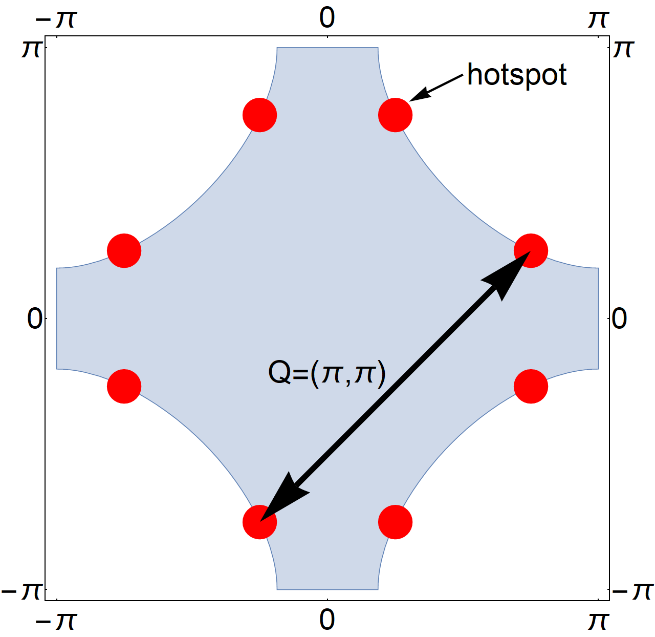
(a)

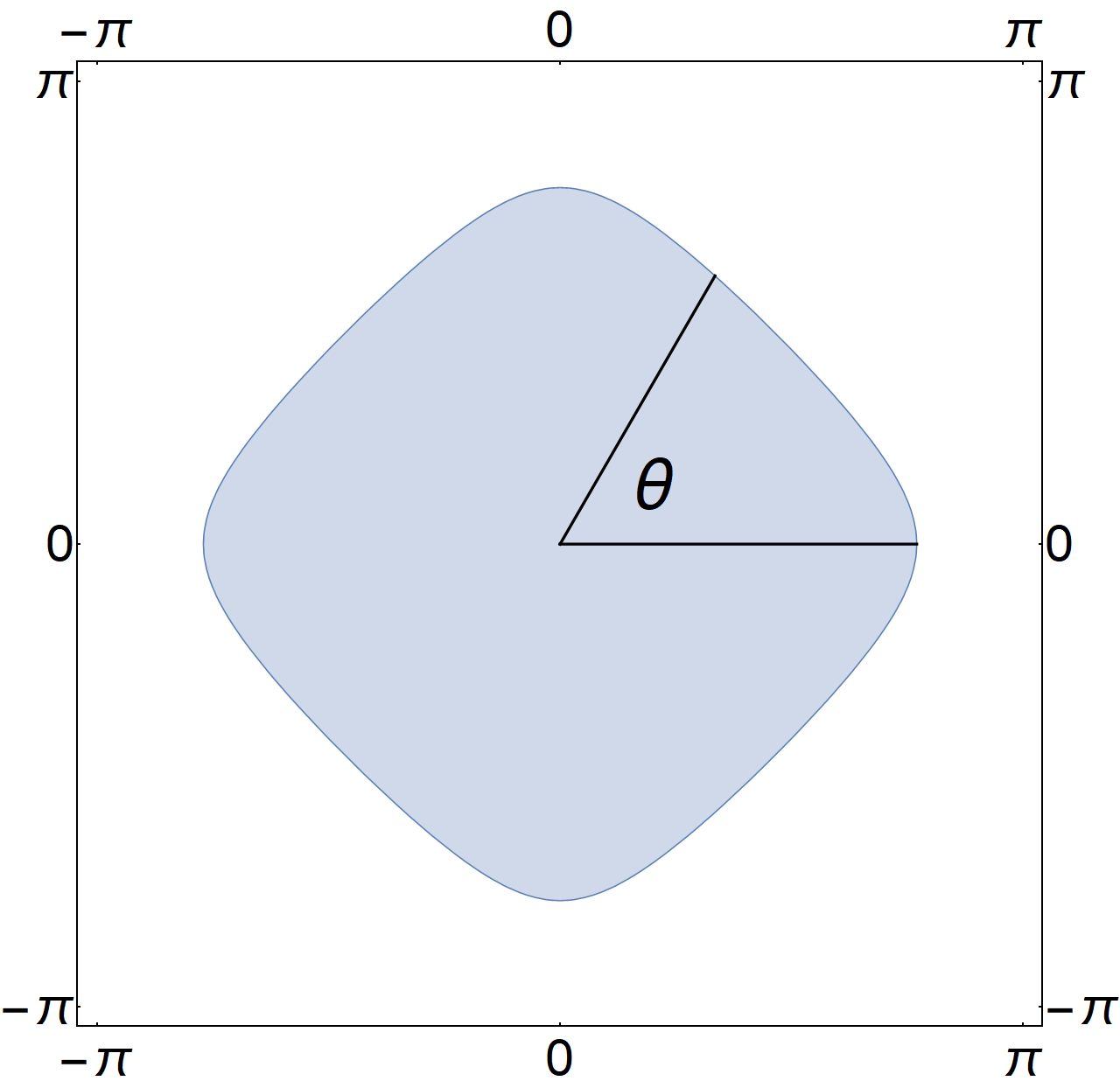
(b)

Figure 1: FS structure of the spin-fermion and Ising-nematic metals. (1(a)) The FS structure of the SFM is 4 hole pockets, with “hotspots” connected by the AF $(\pi,\pi)$ vector. (1(b)) The electron FS in the nematic problem, with the FS angle $\theta$ denoted in the figure.

II.2 Review of the diagrammatic theory

We now briefly review diagrammatic perturbation theory for the two models. The dynamics of fermions and bosons is encoded in their self-energies $\Sigma(\omega,\bm{\mathrm{p}})$ and $\Pi(\Omega,\bm{\mathrm{q}})$ (the latter is also called a polarization bubble). We consider the self-energies on the Matsubara axis, where $\omega=\omega_{m}=2\pi(m+1/2)$ and $\Omega=\Omega_{m}=2\pi m$. As we noted in the Introduction, we compare the results on the Matsubara axis with the QMC data. We use latin letters to denote frequency-momentum 3-vectors, $q=(\Omega_{m},\bm{\mathrm{q}}),k=(\omega_{m},\bm{\mathrm{k}})$. The self-energies are related to bosonic and fermionic propagators as

$$G(k)=\left(i\omega_{m}+i\Sigma(k)-\epsilon(\bm{\mathrm{k}})\right)^{-1}$$ (15)

and

$$D(q)=D_{0}\left(M^{2}_{0}+(\bm{\mathrm{q}}-\bm{\mathrm{Q}})^{2}+\Pi(q)\right)^{-1}$$ (16)

Both self-energies are represented by diagrammatic series in the effective coupling ${\bar{g}}=g^{2}D_{0}$. We assume that ${\bar{g}}$ is small compared to the Fermi energy $E_{F}$. Then we can safely restrict to the lowest-order expansion in $\bm{\mathrm{q}}-\bm{\mathrm{Q}}$ in Eq. (16) and restrict $\bm{\mathrm{k}}$ in Eq. (15) to be near the FS.

Figure 2: Diagrammatic expressions for $\Pi(q)$ (top) and $\Sigma(k)$ (bottom). Solid lines are fully dressed fermion propagators $G(k)$, wavy lines are fully dressed boson propagators $D(q)$, and solid triangles are fully dressed vertex functions.

The diagrammatic expressions for $G(k)$ and $\Pi(q)$ are presented in Fig. 2. Thick lines in this figure are fully dressed $G(k)$ and $D(q)$ and the solid triangles are fully renormalized vertices. In the ET, as well as in several other computational methods, e.g. fluctuation-exchange (FLEX) and dynamical mean-field approximations, vertex corrections are neglected. As stated in the Introduction, for the cases when bosons are collective modes of fermions, there is no small parameter to justify this step, unless one extends the theory to, e.g., a large number of fermionic flavors. Furthermore, vertex corrections coming from low-energy fermions are logarithmically singular. However, in both SFM and INM these corrections are rather small numerically at frequencies above superconducting $T_{c}$, and we proceed by just neglecting them without further discussion. There are also vertex corrections coming from high-energy fermions (the ones with energies of order bandwidth). These corrections are regular and, to first approximation, can be absorbed into the renormalization of the coupling ${\bar{g}}$.

Without vertex corrections, $\Sigma(\bm{\mathrm{k}})$ and $\Pi(\bm{\mathrm{q}})$ are self-consistently expressed as

$$i\Sigma(k) =N_{b}\bar{g}T\sum_{n}\int\frac{d^{2}p}{\left(2\pi\right)^{2}}f^{2}(\bm{\mathrm{k}}+\bm{\mathrm{p}}/2)G\left(p+k\right)D\left(p\right),$$ (17)

$$\Pi(q) =2\bar{g}T\sum_{n}\int\frac{d^{2}p}{\left(2\pi\right)^{2}}f^{2}(\bm{\mathrm{p}}+\bm{\mathrm{q}}/2)G\left(p+q\right)G\left(p\right).$$ (18)

Here the factor $b$ in $\Sigma$ comes from summation over boson components and the factor 2 in $\Pi$ comes from spin summation.

The r.h.s.’s of Eqs. (17) and (18) contain integrals over fermionic momenta. In principle, these integrals are over the whole Brillouin zone. In the ET for fermion-boson models it is further assumed that the contributions from high-energy fermions to the r.h.s. of Eqs. (17) and (18) can be absorbed into ${\bar{g}}$. This renormalization of the coupling is in addition to the ones discussed above due to high energy static vertex corrections. Therefore, we restrict to contributions from only low-energy fermions treating ${\bar{g}}$ in (17) and (18) as the effective, dressed couplings, which include both vertex corrections and the contributions from high-energy fermions to the r.h.s.’s of (17) and (18). The dressed couplings in these two equations are generally not equal, but the non-equivalence only affects the numerical factors in the formulas below, and for simplicity we keep the same ${\bar{g}}$ in the equations for $\Sigma(k)$ and $\Pi(q)$.

The static contribution to the polarization $\Pi(q)$ serves to renormalize the parameters $D_{0}$ and $M_{0}$ in Eq. (16). In particular, it shifts the bosonic mass to

$$M^{2}=M_{0}^{2}-\Pi(\Omega_{m}=0,\bm{\mathrm{q}}=\bm{\mathrm{Q}}).$$ (19)

The dynamical contribution, which gives rise to Landau damping of a boson, can be obtained most straightforwardly by first integrating in Eq. (18) over momentum and then summing up over Matsubara frequencies Abrikosov et al. (1975). We shift the incoming bosonic momentum to the vicinity of the ordering vector $\bm{\mathrm{q}}\to\bm{\mathrm{Q}}+\bm{\mathrm{q}}$, and symmetrize Eq. (18) by shifting $\bm{\mathrm{p}}\to\bm{\mathrm{p}}-\bm{\mathrm{q}}/2$. We linearize the fermionic dispersion near the FS as $\epsilon(\bm{\mathrm{p}}+\bm{\mathrm{Q}}+\bm{\mathrm{q}})\approx\epsilon+\mathbf{v}_{F}\cdot\bm{\mathrm{q}}$, where $\mathbf{v}_{F}$ is the Fermi velocity at $\bm{\mathrm{p}}_{F}+\bm{\mathrm{Q}}$, and $\bm{\mathrm{p}}_{F}(\theta)=k_{F}(\theta)(\cos\theta,\sin\theta)$ is the Fermi vector with FS angle $\theta$. We then replace the momentum integration by an integral over the dispersion, as $d^{2}p\approx d\theta\nu_{F}(\theta)d\epsilon$, where $\nu_{F}(\theta)=k_{F}(\theta)/v_{F}(\theta)$ is the density of states (DOS). We integrate over $\epsilon$ and obtain

$$\Pi(\bm{\mathrm{Q}}+\bm{\mathrm{q}},\Omega_{m})=2i\bar{g}T\sum_{n}\int\frac{d\theta}{2\pi}\nu_{F}(\theta)f^{2}(\theta)\frac{\Theta(\omega_{n}+\Omega_{m})-\Theta(\omega_{n})}{i(\Omega_{m}+\Sigma(\omega_{n}+\Omega_{m})-\Sigma(\omega_{n}))-(\epsilon(\bm{\mathrm{p}}_{F}(\theta)+\bm{\mathrm{Q}}+\bm{\mathrm{q}}/2)-\epsilon(\bm{\mathrm{p}}_{F}(\theta)-\bm{\mathrm{q}}/2))},$$ (20)

In Eq. (20) $\epsilon(\bm{\mathrm{p}}_{F}(\theta)+\cdots)$ should be understood as the dispersion linearized near the FS.

The fermionic self energy for a fermion on the FS, i.e. for $|\bm{\mathrm{k}}|=k_{F}(\theta_{k})$, is obtained by linearizing the dispersion of an internal fermion near the FS as $\epsilon(\bm{\mathrm{k}}+\bm{\mathrm{Q}}+\bm{\mathrm{p}})\approx\epsilon(\bm{\mathrm{k}})+v_{F}(\theta_{k+Q})|\bm{\mathrm{p}}|\cos(\theta-\theta_{k+Q})$, where $\theta_{k+Q}$ is the FS angle of $\bm{\mathrm{k}}+\bm{\mathrm{Q}}$ and $\theta$ is the angle of $\bm{\mathrm{p}}$. Evaluating the angular integral, we obtain

$$\Sigma(k)\approx N_{b}\bar{g}T\sum_{n}\int\frac{|\bm{\mathrm{p}}|dp}{2\pi}\frac{\sigma(\omega_{n})}{\sqrt{(\omega_{n}+\Sigma(\omega_{n}))^{2}+[v_{F}(\theta_{k+Q})]^{2}|\bm{\mathrm{p}}|^{2}}}\frac{f^{2}(\theta_{k+Q/2})}{M^{2}+|\bm{\mathrm{p}}|^{2}+\Pi(|\bm{\mathrm{p}}|\hat{n}(\theta_{k+Q}),\omega_{m}-\omega_{n})},$$ (21)

where $\hat{n}(\theta_{k+Q})=\left.\frac{(-{\mathbf{v}_{F}}_{y},{\mathbf{v}_{F}}_{x})}{v_{F}}\right|_{\theta=\theta_{k+Q}}$ is a unit vector pointing parallel to the FS at the angle $\theta_{k+Q}$. $\sigma(x)$ is the sign function.

Eqs. (20) and (21) form a self-consistent set of equations for the low energy dynamics of fermions near the FS. We next review how they are rendered analytically tractable in the ET.

II.3 Eliashberg theory at $T=0$

The main technical simplification step in ET Altshuler et al. (1994); Chubukov (2005); Abanov et al. (2003); Rech et al. (2006) is the additional assumption that at $T=0$ the typical momentum transfer of a fermion near its mass shell $v_{F}(|\bm{\mathrm{k}}|-k_{F})\sim\omega+\Sigma(\omega)$ is much smaller than the typical momentum transfer of a boson, i.e.

$$|\omega+\Sigma(\omega)|\ll v_{F}|\bm{\mathrm{q}}|,$$ (22)

where $\omega$ is a typical fermionic frequency and $|\bm{\mathrm{q}}|$ is a typical bosonic momentum. As noted above, this allows one to factorize the momentum interaction between directions along and transverse to the FS. In addition, the ET assumes that relevant frequencies are much smaller than $E_{F}$ and integrates over momenta in infinite limits.

We will first show the results within the ET and then discuss its validity for the SFM and the INM.

We begin with the bosonic self-energy. In Eq. (20), the dominant contributions come from regions where $\delta\epsilon=\epsilon(\bm{\mathrm{p}}+\bm{\mathrm{Q}}+\bm{\mathrm{q}}/2)-\epsilon(\bm{\mathrm{p}}-\bm{\mathrm{q}}/2)$ vanishes. This is the source of the different bosonic dynamics for the SFM and INM. In the SFM, $\delta\epsilon$ vanishes near the hotspots as $\delta\epsilon\approx v_{F}(\theta_{hs})Q_{hs}\sin(\theta-\theta_{hs})$, where $\theta_{hs}$ is the FS angle of a hotspot and $Q_{hs}=k_{F}(\theta_{hs})|{\mathbf{v}_{F}}^{2}_{y}-{\mathbf{v}_{F}}^{2}_{x}|/v_{F}^{2}$. Expanding near the hotspots, replacing the Matsubara sum by an integral and integrating, we obtain

$$\Pi^{{\mbox{\tiny SFM}}}(\Omega_{m})\approx{\bar{g}}\frac{\nu_{F}(\theta_{hs})N}{2\pi}\frac{|\Omega_{m}|}{v_{F}(\theta_{hs})Q_{hs}}.$$ (23)

In the INM, $\delta\epsilon\approx v_{F}(\theta)q\cos(\theta-\theta_{q})$ depends strongly on $|\bm{\mathrm{q}}|,\theta_{q}$, and is dominated by $\theta\approx\theta_{q}\pm\pi/2$, yielding

$$\Pi^{{\mbox{\tiny INM}}}(\Omega_{m},\bm{\mathrm{q}})\approx{\bar{g}}\frac{\nu_{F}(\theta_{q})}{\pi}f^{2}(\theta_{q})\frac{|\Omega_{m}|}{v_{F}(\theta_{q})|\bm{\mathrm{q}}|}.$$ (24)

We emphasize that in both cases the result does not depend on fermionic $\Sigma(\omega_{m})$. This is because in ET the polarization bubble is the convolution of two DOS’s, and each DOS $\nu(\omega)=-(\nu_{F}/\pi){\text{I}m}\int d\bm{\mathrm{k}}G(\omega,\bm{\mathrm{k}})=\nu_{F}\sigma(\omega)$ is independent of $\Sigma(\omega)$.

We now turn to the fermionic self-energy. In Eq. (21), we can approximate $(\sqrt{(\omega_{m}+\Sigma(\omega_{m}))^{2}+v_{F}^{2}|\bm{\mathrm{p}}|^{2}})^{-1}\approx(v_{F}|\bm{\mathrm{p}}|)^{-1}$, because of the assumption of ET, Eq. (22). This term then just contributes a factor $\propto|\bm{\mathrm{p}}|^{-1}$ to the integral, which reduces the effective dimensionality of the $\bm{\mathrm{p}}$ integral and renders it one dimensional. Physically this means that the boson momentum $\bm{\mathrm{p}}$ is confined to be parallel to the FS. Then the momentum and frequency integrals are straightforward. For the SFM at the QCP $M=0$ we obtain

$$\Sigma^{{\mbox{\tiny SFM}}}(\omega_{m})\approx\omega_{{\mbox{\tiny SFM}}}^{1/2}|\omega_{m}|^{1/2}\sigma(\omega_{m})$$ (25)

where $\omega_{{\mbox{\tiny SFM}}}=\frac{N_{b}^{2}\bar{g}Q_{hs}}{2\pi Nk_{F}(\theta_{hs})}$, while for the INM we get,

$$\Sigma^{{\mbox{\tiny INM}}}(\omega_{m})\approx\omega_{{\mbox{\tiny INM}}}^{1/3}|\omega_{m}|^{2/3}\sigma(\omega_{m}).$$ (26)

where $\omega_{{\mbox{\tiny INM}}}=\frac{\bar{g}^{2}f^{4}(\theta_{q})}{8\pi^{2}3^{3/2}\nu_{F}(\theta_{q})v_{F}^{2}(\theta_{q})}$.

Now we check the justification of the assumption we made, Eq. (22). Consider first the SFM. In both Eqs. (20) and (21) the Heaviside and sign functions limit internal Matsubara frequencies to be on order of the external frequency. As we discussed in the introduction, both the NFL behavior and superconductivity in the SFM, emerge at typical external frequencies on order of $\omega\sim\omega_{\mbox{\tiny SFM}}\sim\bar{g}/N$, see Eq. (25). In the bosonic self energy, the typical bosonic momentum is $v_{F}Q_{hs}\sim E_{F}$ so the assumption is well justified as long as $\bar{g}\ll E_{F}$. On the other hand, in the fermionic self energy, the typical boson momentum is $v_{F}p\sim\sqrt{\Pi(\omega_{\mbox{\tiny SFM}})}\sim\bar{g}$, so the bosonic and fermionic momenta are of the same order unless $N\gg 1$. In practice, $N=8$ of the SFM is sufficiently large that there is just a reduction of the scale $\omega_{\mbox{\tiny SFM}}$ by a factor of order one. In the INM, the typical frequencies are of order $\omega\sim\omega_{\mbox{\tiny INM}}\sim\bar{g}^{2}/E_{F}\ll E_{F}$, while the typical bosonic momenta are of order $v_{F}p\sim\sqrt{\Pi(\omega_{\mbox{\tiny INM}})}\sim\bar{g}$. Thus, the Eliashberg condition is well obeyed for the INM.

We see that at low enough temperatures, all fermionic self energies scale as power-laws in $\omega_{m}$, with no additional temperature dependence. Therefore, the fermionic self energies at different temperatures should collapse onto one another, and should vanish at the lowest frequencies. Similarly, the bosonic self energies in the SFM should collapse onto one another, while in the INM they should scale with $1/|\bm{\mathrm{q}}|$. In the next section, we show that finite temperature effects destroy these scaling properties.

III Self-energies at finite temperatures

We now turn to study the bosonic and fermionic self energies at finite temperatures. We do not assume that the typical fermionic momentum is smaller than bosonic momentum. In addition, we do not replace the Matsubara sum by a frequency integral, which means that we must account for the thermal piece which we discussed in the Introduction.

We start with the fermionic self-energy. We explicitly split the Matsubara sum into a thermal and nonthermal part and rewrite $\Sigma$ as,

$$\Sigma(\omega_{m})\approx\Sigma_{T}(\omega_{m})+\Sigma_{Q}(\omega_{m}),$$ (27)

where $\Sigma_{T}(\omega_{m})$ contains only the $\omega_{m}=\omega_{n}$ term in the sum, and $\Sigma_{Q}(\omega_{m})$ accounts for the nonthermal dynamical contributions. $\Sigma_{T}$ should be understood as the thermal scattering rate of the fermions, akin to scattering due to static disorder. As a guide for developing a useful approximation, we notice that the Eliashberg $T=0$ results, Eqs. (23–26), are actually the same as what would be obtained without self-consistency, i.e. the Eliashberg approximation reduces to the one-loop result. Therefore, we will assume that the thermal $\Sigma_{T}$ must be evaluated self-consistently, but $\Sigma_{Q}$ does not and only requires the self-consistent $\Sigma_{T}$ as an input. We first present the results and then discuss the validity of the approximation.

The self-energy $\Sigma_{T}$ is the solution of the self-consistent equation

$$\Sigma_{T}(\omega_{m},\theta_{k}) \approx N_{b}\bar{g}T$$

$$\quad\int\frac{|\bm{\mathrm{p}}|dp}{2\pi}\frac{\sigma(\omega_{m})}{\sqrt{(\omega_{m}+\Sigma_{T}(\omega_{m}))^{2}+\tilde{v}_{F}^{2}|\bm{\mathrm{p}}|^{2}}}\frac{f^{2}(\theta_{k})}{m^{2}+|\bm{\mathrm{p}}|^{2}}$$

$$=\frac{\bar{g}Tf^{2}(\theta_{k})\sigma(\omega_{m})}{2\pi|\omega_{m}+\Sigma_{T}(\omega_{m})|}\mathcal{S}\left(\frac{v_{F}M}{|\omega_{m}+\Sigma_{T}(\omega_{m})|}\right),$$ (28)

where

$$\mathcal{S}(x)=\frac{\cosh^{-1}(1/x)}{\sqrt{1-x^{2}}}\approx\left\{\begin{array}[]{ll}\log(2/x)&x\ll 1\\ \pi/(2x)&x\gg 1\end{array}\right..$$ (29)

and $\tilde{v}_{F}=v_{F}(\theta_{k+Q})$, i.e. $\tilde{v}_{F}=|v_{F}(\theta_{hs})|$ for the SFM and $\tilde{v}_{F}=v_{F}(\theta_{k})$ for the INM. Recall that we set $f(\theta)=1$ for the SFM. For the INM, the typical momentum transfers along the FS are small, and this explains the presence of $f^{2}(\theta_{k})$ in the r.h.s. of (III).

We assume that close enough to the QCP, $v_{F}M\ll|\omega_{m}|+|\Sigma_{T}(\omega_{m})|$ for all Matsubara numbers (this will allow us to obtain analytic expressions in what follows). Using the form of $S(x)$ in this limit, we can solve Eq. (III) to obtain an analytic expression for $\Sigma_{T}(\omega_{m})$. For $\omega_{m}>0$,

$$\Sigma_{T}(\omega_{m},\theta_{k})$$

$$\approx\sqrt{\omega_{T}(\theta_{k})^{2}\log\frac{\sqrt{4\omega_{T}(\theta_{k})^{2}+\omega_{m}^{2}}+\omega_{m}}{v_{F}M}+\frac{\omega_{m}^{2}}{4}}-\frac{\omega_{m}}{2}$$

$$=\left\{\begin{array}[]{ll}\omega_{T}(\theta_{k})-\frac{\omega_{m}}{2}&\omega_{m}\ll\omega_{T}(\theta_{k})\\ \frac{\omega_{T}(\theta_{k})^{2}}{\omega_{m}}&\omega_{m}\gg\omega_{T}(\theta_{k})\end{array}\right.$$ (32)

where

$$\omega_{T}(\theta_{k}) =\omega_{T}^{0}|f(\theta_{k})|\sqrt{\log\frac{2\omega_{T}^{0}|f(\theta_{k})|}{v_{F}M}},\omega_{T}^{0}=\sqrt{\frac{N_{b}\bar{g}T}{2\pi}}$$ (33)

and we neglected $\log(\log(\cdots))$ terms. We show the result in Fig. 3. The crossover between the two asymptotic behaviors of $\Sigma_{T}$ occurs at $\omega_{m}\sim\omega_{T}$, i.e., at a typical Matsubara number

$$m_{T}\equiv\frac{\omega_{T}}{T}\sim\sqrt{\frac{\bar{g}}{T}}\sqrt{\log\frac{\sqrt{\bar{g}T}}{v_{F}M}}.$$ (34)

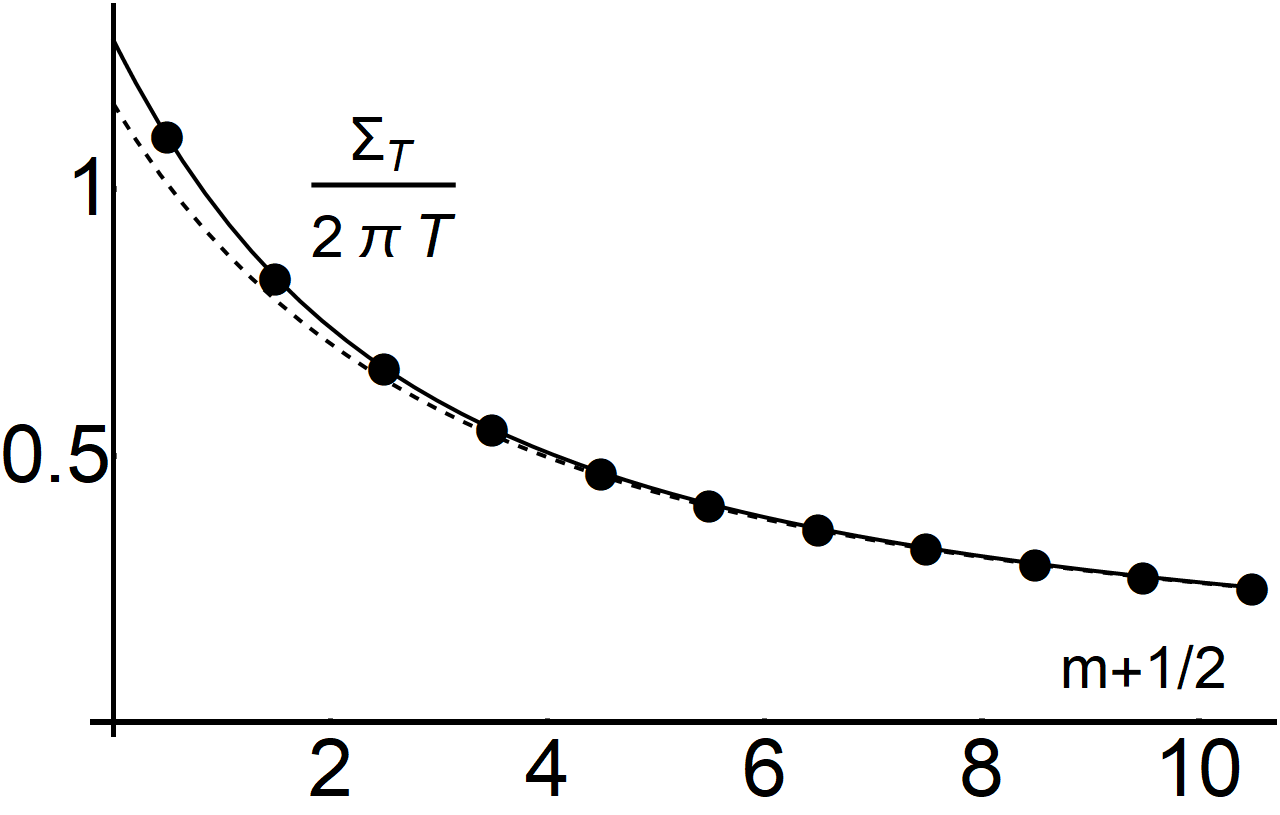
Figure 3: The thermal contribution $\Sigma_{T}(\omega_{m})$ to the fermionic self-energy. The black dots are a numerical solution of Eq. (III). The dashed line is the analytic approximation Eq. (III) and the solid black line is a solution with higher accuracy, up to $\log\log\log(\cdots)$ terms. The numerical solution was obtained for $\frac{2\pi T}{v_{F}M}=\frac{\bar{g}}{2\pi T}=10$.

Next, we determine the dynamic contribution $\Sigma_{Q}$ – the sum over non-zero bosonic frequencies in Eq. (21). As we discussed earlier, this contribution does not require self-consistency as it is sufficient to replace $\Sigma(\omega_{m})$ by $\Sigma_{T}$ in the r.h.s. of (21). For the SFM we find,

$$\Sigma_{Q}^{{\mbox{\tiny SFM}}}(\omega_{m},\theta_{k}=\theta_{hs})\approx\frac{N_{b}\bar{g}T}{2\pi}$$

$$\qquad\sum_{n\neq m}\frac{\sigma(\omega_{n})}{|\omega_{n}+\Sigma_{T}(\omega_{n})|}\mathcal{S}\left(\frac{v_{F}\sqrt{M^{2}+\Pi^{{\mbox{\tiny SFM}}}(\omega_{m}-\omega_{n})}}{|\omega_{n}+\Sigma_{T}(\omega_{n})|}\right),$$ (35)

where $\mathcal{S}(x)$ is the same as in (29), but the argument now contains the polarization bubble $\Pi^{{\mbox{\tiny SFM}}}$ next to $M^{2}$. This implies that the crossover between two limiting forms of $\mathcal{S}(x)$ now holds even if $M=0$, i.e., there are two different behaviors of $\Sigma_{Q}^{{\mbox{\tiny SFM}}}(\omega_{m},\theta_{k})$ near a QCP. To find out at what $m$ the crossover occurs, we need to know $\Pi^{{\mbox{\tiny SFM}}}(\omega_{m}-\omega_{n},Q_{hs})$ at a finite temperature. Examining Eq. (20) for $\Pi(\Omega_{m},Q_{hs})$ we find that corrections to the zero-temperature form, Eq. (23), are suppressed by powers of $T/E_{F}$ and are therefore irrelevant. Therefore, we simply plug the $T=0$ result into (III). We assume and then verify that the argument of $\mathcal{S}$ in (III) is of order one at $m<m_{T}$, where $\omega_{m}<\Sigma_{T}(\omega_{m})$. Neglecting $\omega_{m}$ compared to $\Sigma_{T}(\omega_{m})$, using the fact that typical internal $n$ are comparable to $m$ and using $\Sigma_{T}(\omega_{m})\sim\omega_{T}\sim\sqrt{\bar{g}T\log(\sqrt{{\bar{g}}T}/v_{F}M)}$, $\sqrt{\Pi(\omega_{m}-\omega_{n},Q_{hs})}\sim\sqrt{\nu_{F}\bar{g}\omega_{m}/v_{F}Q_{hs}}$, and $\nu_{F}v_{F}/Q_{hs}=O(1)$, we find that the crossover in $\Sigma_{Q}^{{\mbox{\tiny SFM}}}(\omega_{m},\theta_{hs})$ occurs at $\omega_{m}\sim\omega^{\prime}_{T}\sim\omega_{T}(T/\bar{g})^{1/2}\ll\omega_{T}$, i.e., at a typical Matsubara number

$$m_{T}^{\prime}\sim\log\frac{\sqrt{\bar{g}T}}{v_{F}M}.$$ (36)

Clearly $m_{T}^{\prime}\ll m_{T}$ at low enough temperatures. This justifies the use $m<m_{T}$ in the derivation of (36). The two limiting forms of $\Sigma_{Q}^{{\mbox{\tiny SFM}}}(\omega_{m},\theta_{hs})$ are

$$\Sigma_{Q}^{{\mbox{\tiny SFM}}}(\omega_{m},\theta_{hs})\approx\frac{\bar{g}\omega_{m}}{2\pi^{2}\omega_{T}(\theta_{hs})}L(m,\omega_{m})$$ (37)

at $\omega_{m}\ll\omega_{T}^{\prime}$ , where

$$L\approx\log\left(\frac{\omega_{T}}{v_{F}\sqrt{{\bar{g}}|\omega_{m}|}}\right),$$ (38)

and

$$\Sigma_{Q}^{{\mbox{\tiny SFM}}}(\omega_{m},\theta_{hs})\approx\omega_{{\mbox{\tiny SFM}}}^{1/2}\omega_{m}^{1/2}.$$ (39)

for $\omega_{m}\gg\omega^{\prime}_{T}$. This form is the same as at $T=0$.

We now combine our results for the thermal and quantum parts of the self-energy and show that there are two asymptotic behaviors for $\Sigma(\omega_{m})$ separated by a wide regime.

Region I: the strongly thermal regime –

The strongly thermal regime occurs at $\omega_{m}\ll\omega^{\prime}_{T}\ll\omega_{T}$, i.e., $m\ll m_{T}^{\prime}\ll m_{T}$. In this case, adding up the appropriate limits from Eqs. (III) and (37) we find that the self energy has the form

$$\Sigma^{{\mbox{\tiny SFM}}}(\omega_{m})\approx\omega_{T}\left(1+A\frac{\omega_{m}}{\omega_{T}}\right)$$ (40)

where the leading term comes from frequency-independent part of $\Sigma_{T}$, and the subleading term, with prefactor $A$, is the combination of frequency-dependent term in $\Sigma_{T}$ and from $\Sigma_{Q}$, Eqs. (III) and (37). At vanishing $M$, $A\approx-1/2$, and the full $\Sigma(\omega_{m})$ comes from $\Sigma_{T}$. However, the $O(\omega_{m})$ term from $\Sigma_{Q}$ is only logarithmically reduced and in practice contributes nearly equally to $A$.

Region II: the almost critical regime –

The almost critical regime occurs for $\omega_{m}\gg\omega_{T}\gg\omega^{\prime}_{T}$, i.e., $m\gg m_{T}\gg m_{T}^{\prime}$. Here, summing up the appropriate expressions in Eqs. (III) and (39), we find that the total fermionic self energy has the form

$$\Sigma^{{\mbox{\tiny SFM}}}(\omega_{m})\approx\omega_{{\mbox{\tiny SFM}}}^{1/2}\omega_{m}^{1/2}+\frac{\omega_{T}^{2}}{\omega_{m}}.$$ (41)

The first term (the same one as at $T=0$) comes from $\Sigma_{Q}$, the second one comes from $\Sigma_{T}$. Because $\omega_{{\mbox{\tiny SFM}}}\sim{\bar{g}}$, the first term is the dominant one for $m>m_{T}$, i.e., the self-energy is predominantly determined by dynamical quantum fluctuations.

Note that because $\Sigma_{Q}(\omega_{m})$ changes its behavior at $\omega_{m}\sim\omega_{T}^{\prime}$ and $\Sigma_{T}(\omega_{m})$ changes its behavior at $\omega_{m}\sim\omega_{T}$, there is no single crossover from the region where thermal self energy dominates to the one where the dynamical self energy dominates. In between the two limiting regimes $\omega_{m}\ll\omega^{\prime}_{T}$ and $\omega_{m}\gg\omega_{T}$, there is a wide intermediate region of $\omega^{\prime}_{T}\ll\omega\ll\omega_{T}$, ($m_{T}^{\prime}\ll m\ll m_{T}$), where quantum and thermal contributions are comparable. This is the result we stated in the Introduction, Eq. (5). The implication of Eqs. (41) and (40) is that the behavior of $\Sigma$ at the critical point is quite involved. While at high frequencies the behavior will tend to a power law, at lower frequencies the self-energy saturates and appears to reach a plateau.

Before moving on to the INM, we need to go back and check whether we were justified in neglecting the contribution of $\Sigma_{Q}$ in comparison with $\Sigma_{T}$ in the self-consistent calculation of $\Sigma_{T}$ and subsequent calculation of $\Sigma_{Q}$. From Eqs. (40) and (41), it is evident that in the strongly thermal region $\Sigma_{Q}\ll\Sigma_{T}$ by a logarithmic factor, while in the almost critical regime $\Sigma_{T}\ll\omega_{m}$, and we already know from ET (see Sec. II.3) that the contribution of $\Sigma_{Q}$ can be neglected when computing $\Sigma_{Q}$. In the intermediate regime the approximation is not rigorously justified since both $\Sigma_{T}$ and $\Sigma_{Q}$ scale as $\sqrt{\bar{g}T}$, and both are larger than $\omega_{m}$, but it serves as a way to interpolate between the two regimes.

For the INM, the behavior is somewhat more complex due to the momentum dependence of the polarization. The thermal contribution $\Sigma_{T}(\omega_{m})$ is identical to that for the SFM and is given by Eq. (III). The dynamical contribution is, from Eq. (26),

$$\Sigma_{Q}^{{\mbox{\tiny INM}}}(\omega_{m})\approx\frac{\bar{g}Tf^{2}(\theta_{k})}{2\pi}$$

$$~{}~{}~{}\sum_{n\neq m}\frac{\sigma(\omega_{n})}{|\omega_{n}+\Sigma_{T}(\omega_{n})|}\mathcal{T}\left(\frac{v_{F}M}{p_{n}},\frac{(\Pi^{{\mbox{\tiny INM}}}(\omega_{n}-\omega_{m},p_{n}))^{1/3}}{p_{n}^{2/3}}\right),$$ (42)

where $v_{F}p_{n}=|\omega_{n}+\Sigma_{T}(\omega_{n})|$, $\Pi^{{\mbox{\tiny INM}}}(\Omega_{m},q)$ is given by Eq. (24), and

$$\mathcal{T}(x,y) =\int_{0}^{\infty}\frac{z^{2}dz}{\sqrt{z^{2}+1}(z^{3}+zx^{2}+y^{3})}$$

$$=\left\{\begin{array}[]{lll}\log(2/x)&y=0,x\to 0\\ \log(2/y)&x=0,y\to 0\\ 2\pi/(3\sqrt{3}y)&x=0,y\gg 1\end{array}\right..$$ (46)

A similar analysis to the one we performed for the SFM shows that at $M=0$, $\Sigma_{Q}^{{\mbox{\tiny INM}}}(\omega_{m})$ undergoes a crossover at $\omega^{\prime}_{T}\sim\omega_{T}(\omega^{2}_{T}/({\bar{g}}E_{F}))\sim\omega_{T}(T\log{(\sqrt{{\bar{g}}T}/v_{F}M)}/E_{F})$ between $\Sigma_{Q}^{{\mbox{\tiny INM}}}(\omega_{m})\sim(\omega_{m}/\omega_{T})\log{(\nu_{F}{\bar{g}}\omega_{m}v^{2}_{F}/\omega^{3}_{T})}$ at $\omega_{m}<\omega^{\prime}_{T}$ and $\Sigma_{Q}^{{\mbox{\tiny INM}}}(\omega_{m})\sim\omega^{2/3}_{m}(\omega_{{\mbox{\tiny INM}}})^{1/3}$ at $\omega_{m}>\omega^{\prime}_{T}$. The crossover frequency $\omega^{\prime}_{T}$ is different from the one for the SFM but like in that case, $\omega^{\prime}_{T}\ll\omega_{T}$. Comparing the results for $\Sigma_{Q}^{{\mbox{\tiny INM}}}(\omega_{m})$ and $\Sigma_{T}(\omega_{m})$, Eq. (29), we obtain the limiting forms of $\Sigma^{\mbox{\tiny INM}}$ in region $I$, $\omega_{m}<\omega^{\prime}_{T}$ and region II, $\omega_{m}>\omega_{T}$:

$$\Sigma(\omega_{m})\approx\left\{\begin{array}[]{ll}\omega_{T}\left(1+B\frac{\omega_{m}}{\omega_{T}}\right)&\text{region I}\\ \omega_{{\mbox{\tiny INM}}}^{1/3}\omega_{m}^{2/3}+\frac{\omega_{T}^{2}}{\omega_{m}}&\text{region II}\end{array}\right.,$$ (47)

where $B$ is a constant. (Note that since $\omega_{T}^{\prime}/\omega_{T}\sim\omega_{T}^{2}/\bar{g}E_{F}$, for low enough temperatures $\omega_{T}^{\prime}<T$ and region I is inaccessible.)

We now discuss the bosonic self energy in more detail. From Eq. (20) we see that corrections to the $T=0$ form of $\Pi$ comes from the term $\omega_{m}+\Sigma(\omega_{m})$, which means that the behavior of $\Pi$ depends on whether we are in region I or II. In region II, we may neglect self-energy corrections to $\Pi$ and it will retain its $T=0$ form. In region I, there is a different behavior for the SFM vs. the INM. In the SFM, the typical momentum transfer is of order $v_{F}Q_{hs}\sim E_{F}$, hence $v_{F}Q_{hs}\gg\omega_{T}$ even at finite $T$, and the $T=0$ result holds. In the INM, the typical momentum transfer is $v_{F}|\bm{\mathrm{q}}|\sim(\bar{g}E_{F}T)^{1/3}\gg\omega_{T}$, so the the $T=0$ result can be used in evaluating the fermionic self energy. However, since QMC simulations also measure $\Pi(\Omega_{m},|\bm{\mathrm{q}}|)$ for a given external $\Omega_{m},|\bm{\mathrm{q}}|$, and since there is a large parameter range where $|\omega_{m}|\ll v_{F}|\bm{\mathrm{q}}|\ll\omega_{T}$, we need to calculate $\Pi$ taking into account the self-energy contribution.

For the computation $\Pi$ in the INM, it is important to realize that a nematic order parameter is not a conserved quantity, such as e.g. a spin order parameter (the total magnetization) in a ferromagnet. For a conserved order parameter, a Ward identity insures that within ET vertex corrections cancel out exactly, so that the one-loop calculation which is analogous to Eq. (24) is exact. In the INM this cancelation does not occur, hence at low frequencies self-energy corrections become important. This is true even in the $T=0$ limitPunk (2016).

To gain a qualitative understanding of the impact of the self-energy we evaluate Eq. (20), keeping only the thermal part of the fermionic self-energy. To leading order in $\omega$ we may treat the self-energy as a constant $\Sigma_{T}(\omega_{n},\theta_{k})\approx\omega_{T}(\theta_{k})\sigma(\omega_{n})$. We obtain,

$$\Pi^{in}(\Omega_{m},\bm{\mathrm{q}}) \approx 2i\bar{g}T\sum_{n}\int\frac{d\theta}{2\pi}\nu_{F}(\theta)f^{2}(\theta)\frac{\Theta(\omega_{n+m})-\Theta(\omega_{n})}{i\omega_{T}(\theta)(\sigma(\omega_{n+m})-\sigma(\omega_{n}))-v_{F}(\theta)q\cos(\theta-\theta_{q})}$$ (48)

$$\approx\frac{\bar{g}}{2\pi^{2}}|\Omega_{m}|\int d\theta\nu_{F}(\theta)f^{2}(\theta)\frac{2|\omega_{T}(\theta)|}{4\omega_{T}^{2}(\theta)+v_{F}^{2}(\theta)q^{2}\cos^{2}(\theta-\theta_{q})}$$

$$\approx\bar{g}\frac{\tilde{\nu}_{F}}{2\pi}\frac{|\Omega_{m}|}{\omega_{T}(\theta=0)}$$ (49)

where $\tilde{\nu}_{F}=\left(2\pi\right)^{-1}\int\nu_{F}(\theta)|f(\theta)|$, and the last line is valid for $q\to 0$. The detailed behavior of $\Pi$ as a function of $\Omega_{m},\Sigma(\omega_{m}),q$ and $\theta$ is more complicated and is obtained by a numerical integration of Eq. (48).

Eqs. (III) and (49) for the INM and Eqs. (23) and (37) for the SFM show remarkably similar behavior. The fermionic response is the same for both systems, up to some model-dependent constants. The bosonic response is featureless and linear in $\Omega_{m}$, which implies that the fermionic self-energy will be qualitatively the same as for the SFM in both models.

IV Lattice theory

Before beginning our analysis of the QMC data, we first briefly describe the lattice version of the self consistent equations (17) and (18), which we refer to as the lattice theory (LT). As we discussed there, comparing ET, LT and QMC results gives us insight into the role of high energy fermions in contributing to the self energy.

The SFM and INM are defined on a finite space-time lattice of $L\times L\times L_{\tau}$ sites with periodic boundary conditions in the spatial directions, and periodic (antiperiodic) boundary conditions for the bosons (fermions) in the imaginary time direction. For both models, the bosonic part of the action is given by the lattice version of Eq.(8), with an additional dynamical term

$$\mathcal{S}_{b}=D^{-1}_{0}\int d\tau\sum_{\bm{\mathrm{q}}}\phi(\bm{\mathrm{q}})(M^{2}_{0}-\partial^{2}_{x}-\partial^{2}_{y}-c^{-2}\partial^{2}_{\tau})\phi(\bm{\mathrm{q}}).$$ (50)

Here $\partial_{x,y,\tau}$ is understood as a discretized derivative, and $c$ is the bare velocity of the boson. We introduce this additional dynamical term to better match the QMC lattice models, where the bosonic fields have their own independent dynamics.

In the Ising-nematic case, the form factor is slightly modified compared to the definition used in Sec. II.1,

$$\mathcal{S}_{\mathrm{I}}=\frac{g}{L}\int d\tau\sum_{\mathbf{kq}\sigma}\psi^{\dagger}_{\sigma}(\mathbf{k}-\mathbf{q})\psi_{\sigma}(\mathbf{k})\phi(\mathbf{q})f(\mathbf{k},\mathbf{q}),$$ (51)

where $f(\bm{\mathrm{k}},\bm{\mathrm{q}})=\cos\left(q_{x}/2\right)\cos\left(k_{x}-q_{x}/2\right)-\cos\left(q_{y}/2\right)\cos\left(k_{y}-q_{y}/2\right)=\cos k_{x}-\cos k_{y}+O(q)$.

The self energies then take the form

$$i\Sigma(k)=\frac{g^{2}T}{L^{2}}\sum_{q}f^{2}(\mathbf{k},\mathbf{q})D(q)G(k+q)$$ (52)

$$\Pi(q)=\frac{2g^{2}T}{L^{2}}\sum_{k}f^{2}(\mathbf{k},\mathbf{q})G(k)G(k+q)$$ (53)

The fermionic part of the action is given by Eq. (7), where $\epsilon_{\mathbf{k}}$ is a nearest-neighbor tight-binding dispersion.

In the spin-fermion case, we consider the two-band model depicted in Fig. 4. Again, the reason for this is to better match the sign problem-free model that was simulated in QMC. The fermionic part of the action is

$$\mathcal{S}_{f}=\int d\tau\sum_{\mathbf{k}\eta\sigma}\psi_{\eta\sigma}^{\dagger}(\mathbf{k})(\partial_{\tau}-\epsilon_{\eta,\mathbf{k}})\psi_{\eta\sigma}(\mathbf{k}),$$ (54)

where $\eta=\pm 1$ is the band index.

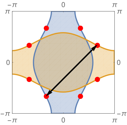
Figure 4: FS structure of the two-band spin-fermion model used in the QMC simulations and the LT calculations. Hotspots are indicated in red, and are connected by the AF wavector $\mathbf{Q}=(\pi,\pi)$, denoted by an arrow.

The interaction part of the action is

$$\mathcal{S}_{I}=\frac{g}{L}\int d\tau\sum_{\mathbf{kq}\sigma\sigma^{\prime}\eta}\vec{\phi}(\mathbf{Q}+\mathbf{q})\psi^{\dagger}_{\eta\sigma}(\mathbf{k})\vec{\tau}_{\sigma\sigma^{\prime}}\psi_{-\eta\sigma^{\prime}}(\mathbf{k}+\mathbf{Q}+\mathbf{q})$$ (55)

Finally, the LT self energies are given by

$$i\Sigma_{\eta}(k)=\frac{g^{2}N_{b}T}{L^{2}}\sum_{q}D(q)G_{-\eta}(k+q),$$ (56)

$$\Pi(q)=\frac{2g^{2}T}{L^{2}}\sum_{k\eta}G_{\eta}(k)G_{-\eta}(k+q).$$ (57)

We solve the LT equations by using the iteration method. The local nature of the boson-fermion coupling allows us to rewrite the Eliashberg equations in real space and imaginary time. We then evaluate the self-energies by performing a fast Fourier transform, with a computational cost of $L^{2}L_{\tau}\log(L^{2}L_{\tau})$ per iteration. Note that a naïve Fourier transform of the fermionic Green’s function to Matsubara frequencies generates an error which scales as $O(1/TL_{\tau})$. For better convergence, we use the ‘Filon-Trapezoidal’ ruleTuck (1967) to reduce the error to $O(1/TL_{\tau})^{2}$.

V Comparison to Lattice theory and to Quantum Monte Carlo simulations

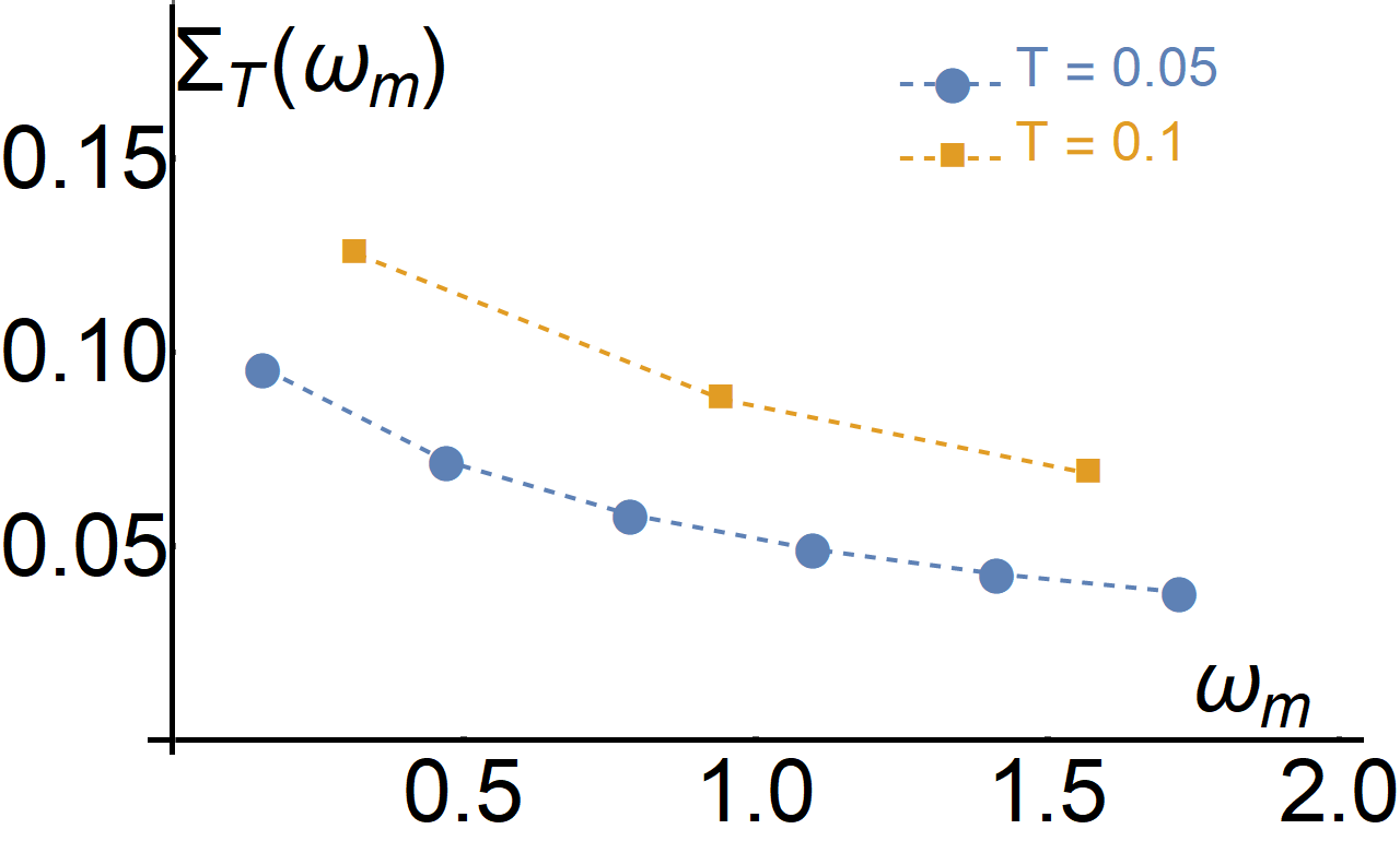
(a)

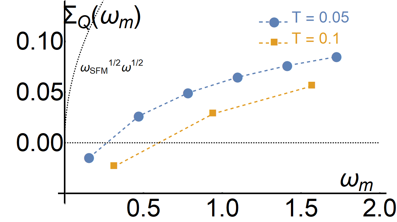
(b)

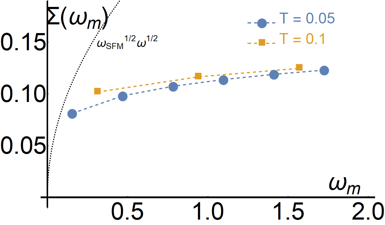
(c)

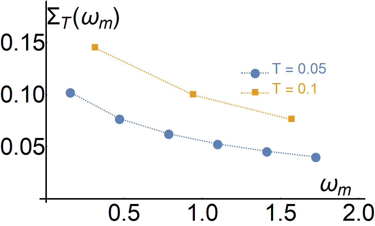
(d)

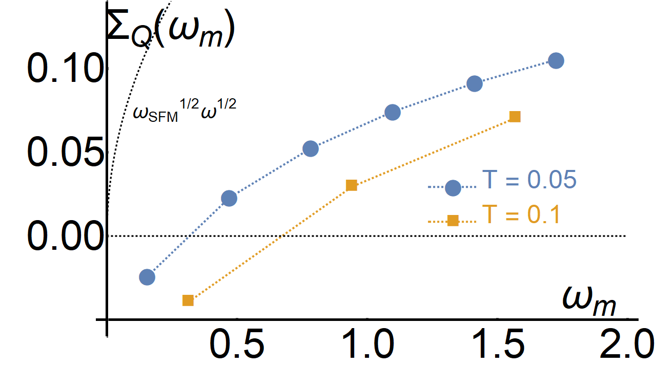
(e)

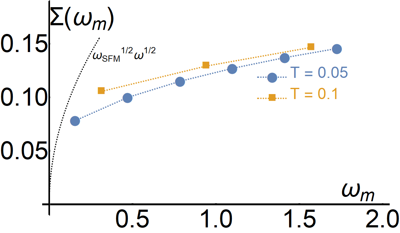
(f)

Figure 5: The fermionic self-energy for the SFM. (a, b, c – dashed traces) Fermionic self energy from MET, Eq. (27), showing the (a) thermal, (b) quantum and (c) total self energy. The black dashed line on the right is the asymptotic $T=0$ prediction of ET. (d, e, f – dotted traces) Fermionic self energy from LT.

In this section, we compare our finite-temperature results for the self-energy with QMC results for the SFM and the INM. We compare QMC results to the expressions for $\Sigma(k)$ and $\Pi(q)$, which we obtained within MET as well as within LT. We will see that the functional forms of $\Sigma(k)$ and $\Pi(q)$ obtained within MET and LT are similar but with some differences. By comparing these three forms of $\Sigma$ and $\Pi$ we are able to both verify the validity of the MET, and identify the strength of vertex corrections, not included into MET and LT, and lattice effects, which are not included in MET but are present in LT.

Before going to a detailed comparison, we discuss the relationship between MET, LT, and QMC calculations, and how to compare them.

The models used in the QMC studies differ from the ones we introduced in Sec. II in several ways. First, in the QMC models the bosonic degrees of freedom have their own dynamics. Nevertheless, at low frequencies, relevant to the physics near the QCP, the leading term in the bosonic dynamics is the Landau damping due to coupling to electronic degrees of freedom. This is since the Landau damping term scales as $|\Omega|$, while the dynamical term of a boson scales as $\Omega^{2}$. Second, the models used in the QMC studies contain additional interactions, which are not present in the MET or LT. These include boson-boson interactions, as well as (in the INM) additional, non-critical bosonic modes which couple to the fermions. Finally, the three methods differ in the proper definition of the parameters of $D_{0}$, $M(T)$ and $g$. The QMC starts from the theory with bare parameters and returns the numerically exact $G(k),D(q)$, so that $D_{0},M(T)$ are outputs of the calculation. In the MET and LT, $D_{0},M(T)$ are considered as inputs to the theory. The bare parameter values are renormalized by vertex corrections and, in the case of MET, one-loop self-energy corrections from high-energy fermions. These renormalizations should be absorbed into the input to the theory. This implies that the effective $g$ may be different in MET and LT. We obtain $D_{0}$ and $M(T)$ by fitting the static $D(q,\Omega_{m}=0)$ from QMC, and use the bare value of $g$, as elaborated below. We find that the bare $g$ reproduces the QMC data well for both the SFM and INM.

We first show our results for the SFM. Refs. Schattner et al., 2016a; Gerlach et al., 2017; Berg et al., 2019 presented extensive QMC data on a realization of the SFM. To compare with our work, we use the data from those papers for $g=1.5,T=0.05\ldots 0.2$, where all energies are in units of the bare hopping used in Refs. Schattner et al., 2016a; Gerlach et al., 2017; Berg et al., 2019. We note that for lowest temperature, $T=0.05$, the thermal scale, given by Eq. (33), $\omega_{T}^{0}=0.16$, is almost the same as the lowest Matsubara frequency $\pi T$, and in addition $v_{F}M(T)\gtrsim\pi T,\omega_{T}^{0}$. The implication is that the QMC data mostly fall into the the intermediate regime between regions I and II, and the system is not fully critical. For this reason, for the quantitative comparison of the low-energy MET with QMC we performed the Matsubara summations in Eq. (III) numerically.

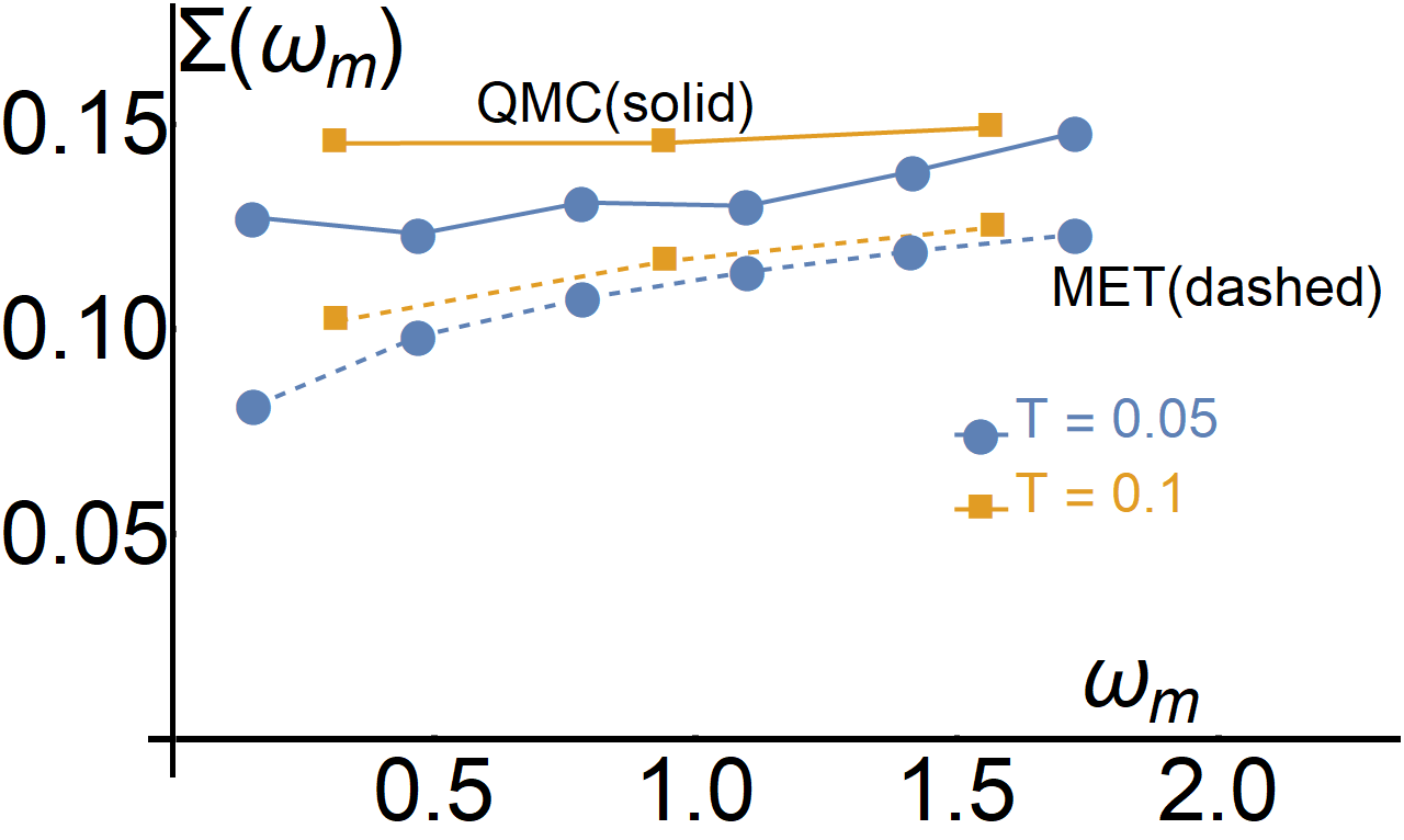
(a)

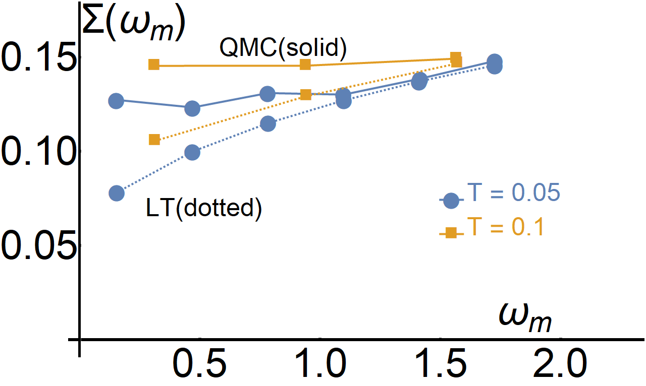
(b)

Figure 6: Fermionic self energies in the SFM. (a) Comparison of the MET and QMC self energy. (b) Comparison of the LT and QMC self energy.

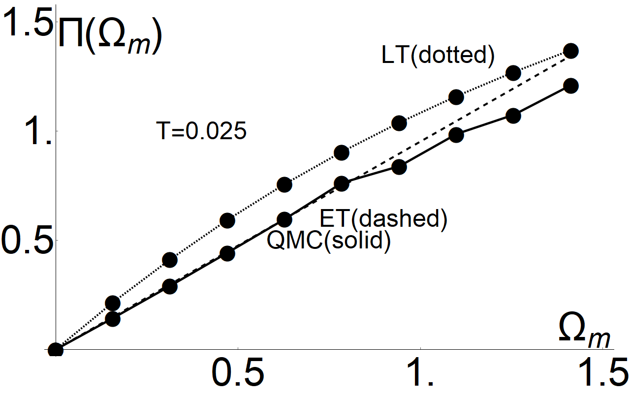
Figure 7: The bosonic self-energy $\Pi(\Omega_{m})$ in the SFM for $q=0$. In this figure, the dashed trace corresponds to the $T=0$ (ET) expression, Eq. (23).

We begin by comparing the self-energies $\Sigma_{T}(\omega_{m})$ and $\Sigma_{Q}(\omega_{m})$ within MET and LT. Fig. 5 presents $\Sigma_{T},\Sigma_{Q}$ and $\Sigma$ at $\theta=\theta_{hs}$ for both methods. Although there are some deviations, the overall results are similar. We also note the somewhat curious feature, shown in panels 5b and 5e, that for both theories the quantum self energy at the first Matsubara frequency $\Sigma_{Q}(\pi T)$ is negative (it is also true for the INM, Figs. 8b, e). We explain this property of $\Sigma_{Q}(\pi T)$ in the Appendix.

In Fig. 6 we compare the QMC data with both calculations. Except for a global discrepancy of about 20% for the MET, and a slight difference in slope for the LT, there is good agreement with QMC. The overall magnitude agrees well, and both the MET and the LT reproduce the QMC result that $\Sigma$ seems to extrapolate to a non-zero value as $\omega_{m}\to 0$. We note that the overall good agreement between MET, LT, and QMC calculations holds despite the fact that the coupling constant $\bar{g}\approx 1.67$ is not small compared to $E_{F}\approx 2.2$, implying e.g. vertex corrections should generally be $O(1)$. In Figs. 5 6 we show only two of the temperatures so as to keep the images clear, but the same agreement holds for the other temperatures. For completeness, we also display a comparison of QMC, MET and LT for $\Pi(\Omega_{m})$ in Fig. 7, showing good agreement.

Next we consider the INM. While in the spin-fermion case, the model used in QMC allows us to directly read off the bare value for the coupling constant $g$, the nematic modes in the QMC studies Schattner et al., 2016b; Lederer et al., 2017; Berg et al., 2019 consist of pseudo-spin $1/2$ degrees of freedom that are located on the bonds of the lattice, and do not directly match the form of Eqs (14,51). Nevertheless, the bare $g$ can be obtained by comparing the interaction term for a uniform ($\bm{\mathrm{q}}=0$) configuration of the nematic modes. This yields $g=3.3\alpha$ for MET and $g=2\alpha$ for the LT, where $\alpha$ is the coupling to the pseudo-spin degrees of freedom in the notation of Refs. Schattner et al., 2016b; Lederer et al., 2017; Berg et al., 2019.

Here, we focus on the data for $\alpha=1$ and $T=0.1,0.167,0.25$. Extracting $D_{0}$ from the QMC data, we find the bare coupling used in MET is $\bar{g}=g^{2}D_{0}=8.25$. We note in passing that QMC simulations show a $T_{c}=0.04$, which is in good agreement with the ET prediction of $T_{c,{\mbox{\tiny ET}}}=0.066$ for the given $\bar{g}$. The Eliashberg $T_{c}$ in the INM scales as $\bar{g}^{2}/E_{F}\propto g^{4}$, so that the difference in critical temperatures can be interpreted as a 15% renormalization of $g$. In the LT, we find $T_{c,{\mbox{\tiny LT}}}=0.03$. 8.

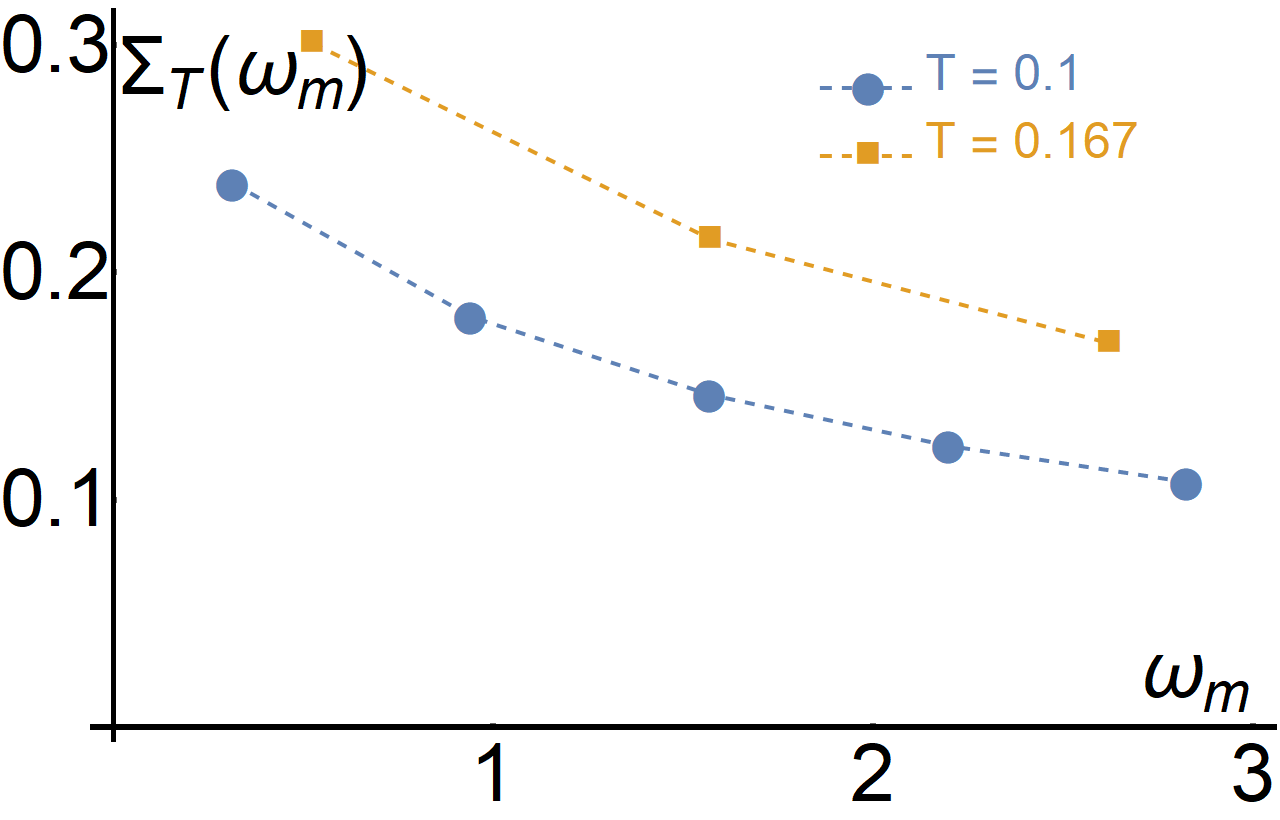
(a)

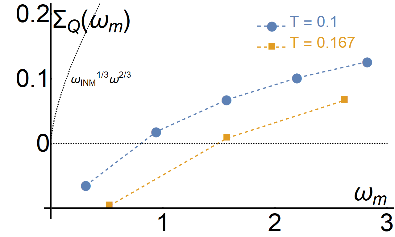
(b)

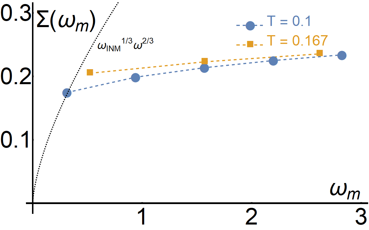
(c)

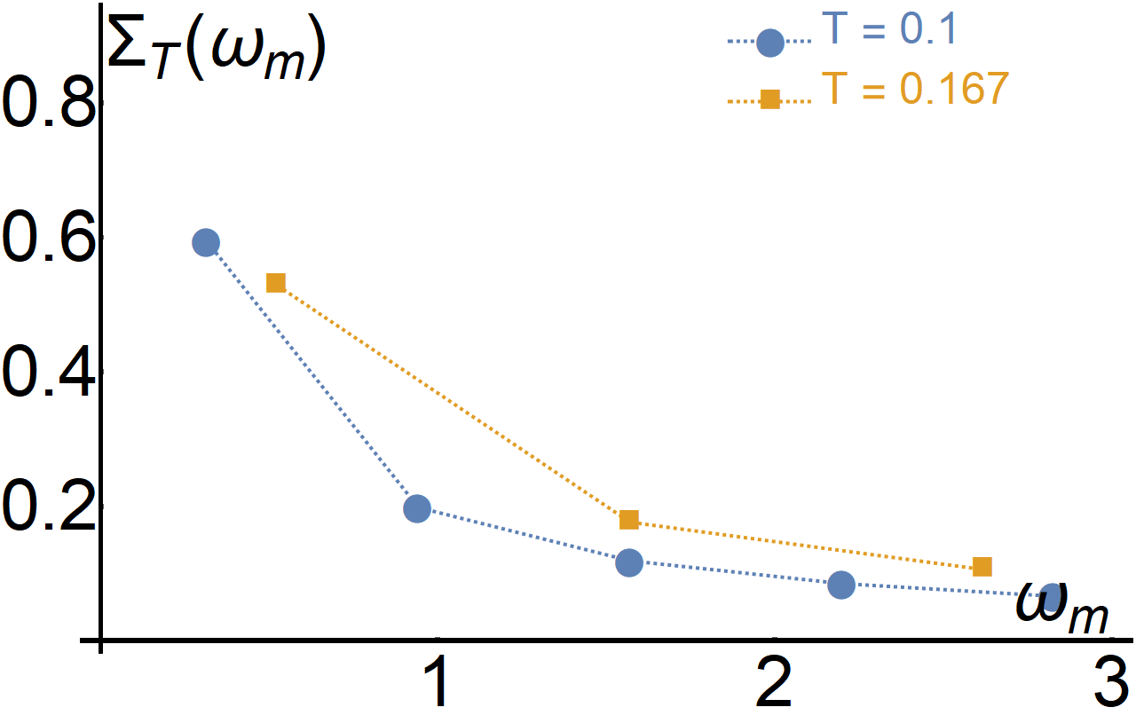
(d)

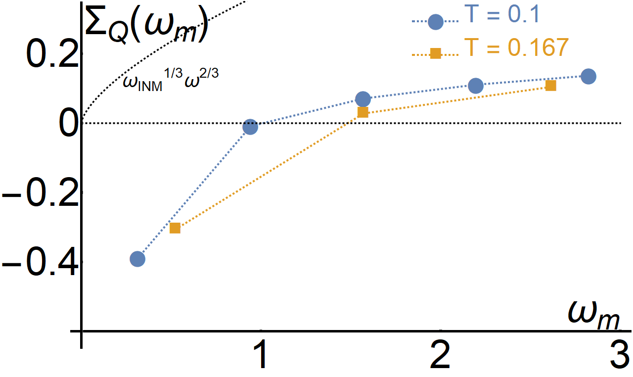
(e)

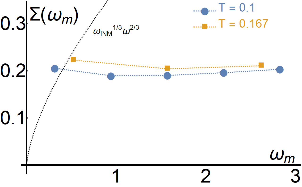
(f)

Figure 8: The fermionic self-energy for the INM. (a, b, c – dashed traces) Fermionic self energy from MET, showing the (a) thermal, (b) quantum and (c) total self energy. The black dashed lines on the right are the asymptotic $T=0$ prediction of ET. (d, e, f – dotted traces) Fermionic self energy from LT.

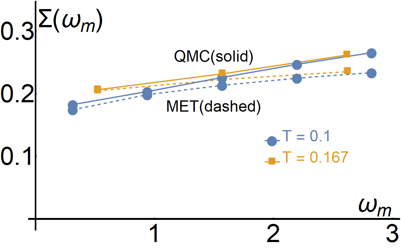
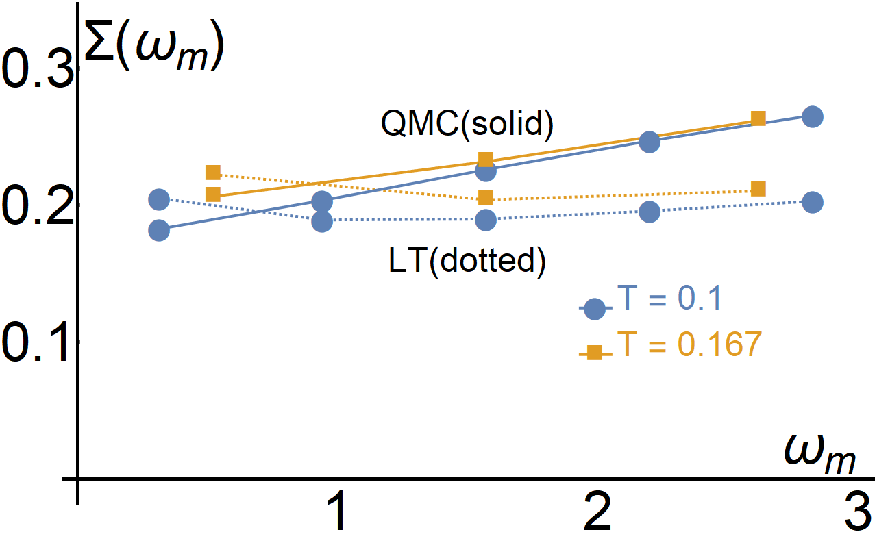
(a)

Figure 9: Fermionic self-energy of the INM. (a) Comparison of the MET and QMC self energy. (b) Comparison of the LT and QMC self energy.

Fig. 9 presents a comparison of the QMC data for $\Sigma$ with both the MET and LT calculations. The MET calculation shows an excellent agreement with the data. The LT calculation has some systematic deviations in the frequency behavior. From all these results, we conclude that similarly to the SFM there are only moderate high-energy vertex corrections and lattice renormalizations in the INM, and that they are somewhat better accounted for in the low energy MET.

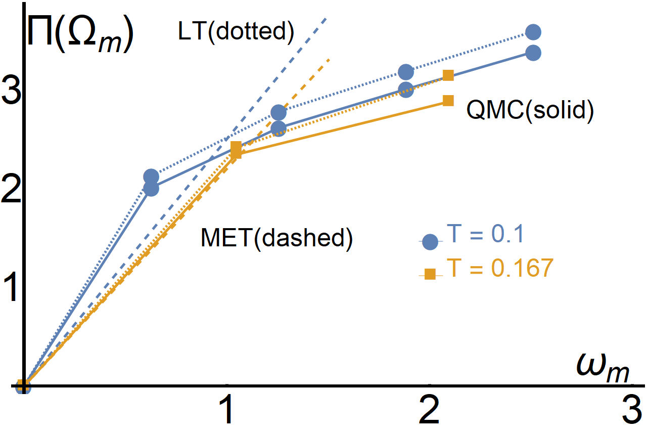
Figure 10: The bosonic self energy $\Pi(\Omega_{m})$ in the INM for the lowest $q=2\pi/L$, where $L$ is the system size. Solid lines denote the QMC data, and dashed and dotted lines denote the MET and LT calculations.

We also compared MET and lattice calculations to the QMC data for $\Pi(q)$. In Fig. 10 we present the behavior of $\Pi$ at the lowest $q=2\pi/L$, where $L$ is the QMC system size, along with a lattice calculation of $\Pi$ and the MET prediction of the low frequency behavior of $\Pi$, Eq. (49). There is good agreement between MET/LT and the QMC data.

We find it striking that most of the features of the QMC data are reproduced by our ET/MET calculations. We believe that our results imply the QMC data is a validation of, rather than a challenge to, the applicability of ET to quantum-critical models of interacting electrons.

We used the differences between the theories to identify the importance of high energy vertex and lattice renormalizations to the low energy theory. The fact that the bare $\bar{g}$ reproduces both $T_{c}$ and the self energy well in both models implies that the contribution to fermionic self-energies from vertex corrections due to high-energy fermions are likely small. In addition, we show that MET reproduces the QMC self energies quite well, but the comparison of QMC with LT shows some systematic deviations. This suggests that there is at least a partial cancellation between vertex corrections and the contribution from high-energy fermions to one loop self-energy.

VI Summary

In this work, we studied the effect of thermal fluctuations on metals near a QCP, either to a spin density wave state or to an Ising nematic state. We calculated the deviation from the scaling behavior predicted by ET, in the regime where the thermal contributions do not permit a separation of scales between fermionic and bosonic degrees of freedom. We found, that at low temperatures, close to the QCP the thermal contribution to fermionic self energy scales as $\omega_{T}\propto\sqrt{\bar{g}T}$ and dominates the contribution from quantum dynamics. We showed that once this additional physics is taken into account, by an appropiately modified Eliashberg theory, it reproduces properties that were found in recent QMC simulations, above the superconducting $T_{c}$.

In the absence of pair-breaking, the regime of metallic quantum critical behavior is limited by the large enhancement of the superconducting $T_{c}$ near the QCP, and the associated strong superconducting fluctuations. QMC studies report no clear separation between the energy scales associated with superconductivity and NFL behavior. As we discussed in the Introduction, this is in agreement with the predictions of ET, where both superconductivity and NFL appear on a scale of $\omega_{\mbox{\tiny SFM}},\omega_{\mbox{\tiny INM}}$ for the SFM and INM respectively. Recent work has indicated Chubukov et al. (2019) that superconducting fluctuations play a significant role in the normal state. Our analysis of the normal-state self neglects superconducting fluctuations, and so the combined effect of thermal and superconducting fluctuations remains an open question. We hope our findings will motivate further numerical and analytic work on quantum critical metals.

Appendix: Quantum self energy at the first Matsubara frequency

In this Appendix we explicitly compute the value of the quantum part of the self energy at the first Matsubara frequency $\Sigma_{Q}(\pi T)$. Our purpose is to justify the somewhat puzzling result, shown in Figs. 5 and 8, that $\Sigma_{Q}(\pi T)$ is negative. We will show that $\Sigma_{Q}(\pi T)$ in MET is always negative, and that this is a consequence of the so-called “first Matsubara frequency rule” - namely that $\Sigma_{Q}(\pi T)=0$ in ET Chubukov and Maslov (2012, 2017).

We assume that we are at the QCP ($M=0$) and write down an expression for $\Sigma_{Q}(\pi T)$ directly from Eq. (21),

$$\Sigma_{Q}(\pi T) \approx\bar{g}T\sum_{n\neq 0}\int_{0}^{\infty}\frac{|\bm{\mathrm{p}}|dp}{2\pi}\frac{\sigma(\Omega_{n}+\pi T)}{\sqrt{(\Omega_{n}+\pi T+\Sigma(\Omega_{n}+\pi T))^{2}+v_{F}^{2}|\bm{\mathrm{p}}|^{2}}}\frac{1}{|\bm{\mathrm{p}}|^{2}+\Pi(|\bm{\mathrm{p}}|,\Omega_{n})},$$

$$=\bar{g}T\sum_{n\geq 1}\int_{0}^{\infty}\frac{|\bm{\mathrm{p}}|dp}{2\pi}\frac{1}{|\bm{\mathrm{p}}|^{2}+\Pi(|\bm{\mathrm{p}}|,\Omega_{n})}\left(\frac{1}{\sqrt{(\Omega_{n}+\pi T+\Sigma(\Omega_{n}+\pi T))^{2}+v_{F}^{2}|\bm{\mathrm{p}}|^{2}}}-\right.$$

$$\qquad\qquad\qquad\qquad\qquad\qquad\qquad\qquad\qquad\qquad\qquad\qquad\left.\frac{1}{\sqrt{(\Omega_{n}-\pi T+\Sigma(\Omega_{n}-\pi T))^{2}+v_{F}^{2}|\bm{\mathrm{p}}|^{2}}}\right),$$ (58)

For simplicity we set $v_{F}(\theta)=v_{F}$, $\nu_{F}(\theta)=\nu_{F}$, $f(\theta)=1$ and $N_{b}=1$.

It is immediately evident that if we neglect the dynamical part in the square-root of the denominator of Eq. (Appendix: Quantum self energy at the first Matsubara frequency) as is done in ET (see Sec. II.3) we obtain $\Sigma_{Q}(\pi T)=0$, because contributions from positive and negative frequencies exactly cancel out. This is the first Matsubara frequency rule. The correction coming from MET is therefore coming from the small asymmetry between positive and negative frequencies that arise from the non-factorization of momentum integration, see the discussion in the Introduction and in Sec. II.3. To proceed we assume and then verify that (i) the integration and summation in (Appendix: Quantum self energy at the first Matsubara frequency) are dominated by large $v_{F}p,\Omega_{n}\gg\pi T$, and that (ii) we may neglect the self-energy terms. Expanding the square-roots we obtain,

$$\Sigma_{Q}(\pi T)\approx-\frac{\bar{g}T}{2\pi}\sum_{n\geq 1}\int_{0}^{\infty}\frac{|\bm{\mathrm{p}}|dp}{|\bm{\mathrm{p}}|^{2}+\Pi(|\bm{\mathrm{p}}|,\Omega_{n})}\frac{2\pi T\Omega_{n}}{(\Omega_{n}^{2}+(\pi T)^{2}+v_{F}^{2}|\bm{\mathrm{p}}|^{2})^{3/2}}$$ (59)

We first solve for the SFM. Here $v_{F}^{2}\Pi^{\mbox{\tiny SFM}}(|\bm{\mathrm{p}}|,\Omega_{n}|)=\omega_{b}\Omega_{n}$ where $\omega_{b}=\frac{\bar{g}N\nu_{F}v_{F}}{2\pi Q_{hs}}$ (by order of magnitude, $\omega_{b}\sim{\bar{g}}$). Rescaling the $p$ integral, we find

$$\Sigma_{Q}^{\mbox{\tiny SFM}}(\pi T)\approx-\frac{\bar{g}T}{2\pi}\sum_{n\geq 1}\int_{0}^{\infty}\frac{xdx}{x^{2}+\frac{\omega_{b}\Omega_{n}}{\Omega_{n}^{2}+(\pi T)^{2}}}\frac{2\pi T\Omega_{n}}{(\Omega_{n}^{2}+(\pi T)^{2})^{3/2}(x^{2}+1)^{3/2}}.$$ (60)

By inspection, one may verify that the integral is dominated by $x\sim 1,\Omega_{n}\sim\omega_{b}$. Since $\omega_{b}$ is a large parameter in the theory, this justifies our previous assumptions, and also allows us to safely replace the summation with an integral. We then obtain

$$\Sigma_{Q}^{\mbox{\tiny SFM}}(\pi T) \approx-\frac{\bar{g}T}{2\pi}\int_{\pi T}^{\infty}\frac{d\Omega}{\Omega^{2}}\int_{0}^{\infty}\frac{xdx}{\left(x^{2}+\frac{\omega_{b}}{\Omega}\right)(x^{2}+1)^{3/2}}$$

$$\approx-\frac{\bar{g}T}{2\pi\omega_{b}}\log\frac{\omega_{b}}{\pi T}$$ (61)

We see that $\Sigma_{Q}^{\mbox{\tiny SFM}}(\pi T)$ is negative and of order ${\bar{g}}T/\omega_{b}\sim T$. For other Matsubara frequencies, $\omega_{n}=O(T)$, and $\Sigma_{Q}^{\mbox{\tiny SFM}}(\omega_{n})$ is positive and of order $(T\omega_{{\mbox{\tiny SFM}}})^{1/2}\sim(T{\bar{g}})^{1/2}\sim T(\bar{g}/T)^{1/2}$, i.e., is much larger than $\Sigma_{Q}^{\mbox{\tiny SFM}}(\pi T)$.

For the INM, we write $v_{F}^{2}\Pi^{{\mbox{\tiny INM}}}(|\bm{\mathrm{p}}|,\Omega_{n})=\omega_{b^{\prime}}^{2}\frac{\Omega_{n}}{v_{F}|\bm{\mathrm{p}}|}$, where $\omega_{b^{\prime}}^{2}=\bar{g}\nu_{F}v_{F}^{2}/\pi$ (by order of magnitude $\omega_{b^{\prime}}\sim({\bar{g}}E_{F})^{1/2}$). Repeating the same computational steps we find,

$$\Sigma_{Q}^{\mbox{\tiny INM}}(\pi T)\approx-\frac{\bar{g}T}{2\pi}\sum_{n\geq 1}\int_{0}^{\infty}\frac{x^{2}dx}{x^{3}+\frac{\omega_{b^{\prime}}^{2}\Omega_{n}}{(\Omega_{n}^{2}+(\pi T)^{2})^{3/2}}}\frac{2\pi T\Omega_{n}}{(\Omega_{n}^{2}+(\pi T)^{2})^{3/2}(x^{2}+1)^{3/2}}.$$ (62)

Again, we find $x\sim 1,\Omega_{n}\sim\omega_{b^{\prime}}$ justifying our assumptions. Replacing the summation by an integral we obtain,

$$\Sigma_{Q}^{\mbox{\tiny INM}}(\pi T) \approx-\frac{\bar{g}T}{2\pi}\int_{\pi T}^{\infty}\frac{d\Omega}{\Omega^{2}}\int_{0}^{\infty}\frac{x^{2}dx}{\left(x^{3}+\frac{\omega_{b^{\prime}}^{2}}{\Omega^{2}}\right)(x^{2}+1)^{3/2}}$$

$$\approx-\frac{\bar{g}T}{4\sqrt{\pi}\omega_{b^{\prime}}}\Gamma^{2}(3/4),$$ (63)

and $\Gamma(3/4)=1.23$. We see that $\Sigma_{Q}^{\mbox{\tiny INM}}(\pi T)$ is again negative. For the INM it is of order $T{\bar{g}}/\omega_{b^{\prime}}\sim T\left({\bar{g}}/E_{F}\right)^{1/2}$. For other Matsubara frequencies $\omega_{n}=O(T)$, $\Sigma_{Q}^{\mbox{\tiny INM}}(\Omega_{n})$ is positive and is of order $(T^{2}{\bar{g}}^{2}/E_{F})^{1/3}\sim\left(T\left({\bar{g}}/E_{F}\right)^{1/2}\right)\left({\bar{g}}E_{F}/T^{2}\right)^{1/6}$, i.e., is again much larger than $\Sigma_{Q}^{\mbox{\tiny INM}}(\pi T)$.