Enhanced models for the nonlinear bending of planar rods: localization phenomena and multistability
1 Department of Civil and Industrial Engineering
University of Pisa, Pisa, Italy
matteo.brunetti@unipi.it
2 Department of Structural and Geotechnical Engineering
Sapienza University of Rome, Rome, Italy
antonino.favata@uniroma1.it
3 Department of Structural and Geotechnical Engineering
Sapienza University of Rome, Rome, Italy
stefano.vidoli@uniroma1
Abstract
We deduce a 1D model of elastic planar rods starting from the Föppl–von Kármán model of thin shells. Such model is enhanced by additional kinematical descriptors that keep explicit track of the compatibility condition requested in the 2D parent continuum, that in the standard rods models are identically satisfied after the dimensional reduction. An inextensible model is also proposed, starting from the nonlinear Koiter model of inextensible shells. These enhanced models describe the nonlinear planar bending of rods and allow to account for some phenomena of preeminent importance even in 1D bodies, such as formation of singularities and localization (d-cones), otherwise inaccessible by the classical 1D models. Moreover, the effects of the compatibility translate into the possibility to obtain multiple stable equilibrium configurations.
Keywords: dimensional reduction, rod theory, d-cone, localization, multistability
1 Introduction
In this paper we intend to propose two mathematical models of a class of bodies that are thin and slender at the same time, a feature that allows to have recourse to a 1D theory. The moderately large deflection of thin elastic plates or shells, i.e., bodies which are intrinsically thin, can be well described by the Föppl–von Kármán (FvK) model [24, 44][13, 15]. Because of the smallness parameter given by the thickness, such a model is intrinsically 2D.
On the side of slender bodies, besides the classical rod models, in the literature are often adopted a number of refinements, many of them having the scope to go beyond the limits of the standard rod models, such as Timoshenko’s or Euler’s.
A full description of the huge literature on the subject is unattainable; we here quote [18, 19, 42, 32] and, among the most recent works [30, 2, 34, 29, 4, 35, 36, 11]. In particular, in [4] a model for rods and thin-walled rods is rigorously obtained from a formal asymptotic analysis of three-dimensional linear elasticity. In [36] a general method for deriving one-dimensional models for nonlinear structures has been proposed; the models capture the contribution to the strain energy arising not only from the macroscopic elastic strain, but also from the strain gradient. Moreover, the so-called models à la Sadowsky, usually generated starting from plate models, are sometimes adopted. Among these, the original one proposed by Sadowsky in 1930 [41] and formally justified by Wunderlich in 1962 [45], has been deduced from the linear Kirchhoff plate model. Recently, similar models have been deduced from the non-linear von Kármán plate model [25, 26]; the limit problems penalize extensional, flexural and torsional deformation and they are comparable to classical non-linear rod theories.
In [27, 28] a hierarchy of one-dimensional models for thin-walled rods with rectangular cross-section, starting from three-dimensional nonlinear elasticity has been deduced. The different limit models are distinguished by the different scaling of the elastic energy and of the ratio between the sides of the cross-section.
In [22, 23] the authors consider a rod whose cross section is a tubular neighborhood, with thickness scaling with a parameter , of a simple curve whose length scales with ; to model a thin-walled rods they assume that goes to zero faster than , and they measure the rate of convergence by a slenderness parameter. The approach recovers in a systematic way, and gives account of, many features of the rod models in the theory of Vlasov.
In this paper, we deduce two 1D models of elastic rods enhanced by additional kinematical descriptors that keep explicit track of the compatibility condition requested in the 2D parent continua; in the classical models this condition is identically satisfied after the dimensional reduction. The models differ for the possibility to account or not for extensibility. They allow to describe some phenomena of preeminent importance in non-linear elasto-statics, such as formation of singularities and localization of the elastic energy (d-cones, elastic folds, etc.), otherwise inaccessible by the classical 1D models. Indeed, these phenomena are expression of a complex interaction between elasticity and geometry having an intrinsically 2D character, the compatibility conditions being the formal expression of such interaction. In the FvK model, e.g., the compatibility condition descends from the Gauss Theorema Egregium and expresses the relation between membrane deformations and variation of Gaussian curvature and, on selecting the isometries, identifies those changes of configuration that are energetically favorable. Moreover, the 1D compatibility condition, by introducing a strong non-linearity in the problem, induces the possibility to have multiple stable solutions, in accordance with experimental evidence [9, 8].
The paper is organized as follows. In Sec. 1.1, the prototypical problem we intend to face is described in detail. In Sec. 2 we present a dimensional reduction to obtain a rod model starting from a 2D inextensible shell model; the problem translates into a constrained minimization, in terms of two kinematical decriptors, i.e., the axial and the transversal curvatures. The compatibility condition is nothing but a suitable version of the inextensibility constraint.
In Sec. 3 we present a dimensional reduction starting from the FvK model. We obtain a non-local model, governed by three scalar fields: the axial and the transversal curvatures, and the 1D counterpart of the stress Airy function. As it happens in the FvK model, these fields are not independent and the 1D compatibility prescribes how they have to be related.
Sec. 4 is devoted to results. Solving the inextensible problem translates into a simple geometric equivalent construction, that allows to obtain analytical results: the constrained energy minimization problem is reduced to find a sequence a points on a three-dimensional cone, having minimal total distance from a given point, representing the stress-free configuration. Analytical solutions are not possible for the extensible case, and we then use a finite element method to solve the problem. We then present a comparison between the results obtained with the two enhanced rod models here formulated and the FvK predictions, in terms of displacements and stresses.
Discussions and conclusions are in Sec. 5. In particular, we discuss the role of the 1D compatibility condition, showing that it is crucial to capture multistability: besides the configuration with a localized axial curvature, a second configuration is predicted, in which the transversal curvature is null and the axial one is constant. This is in agreement with numerical results obtained with the FvK model and experimental evidence already discussed and published by some of the authors [8].
1.1 Problem set-up
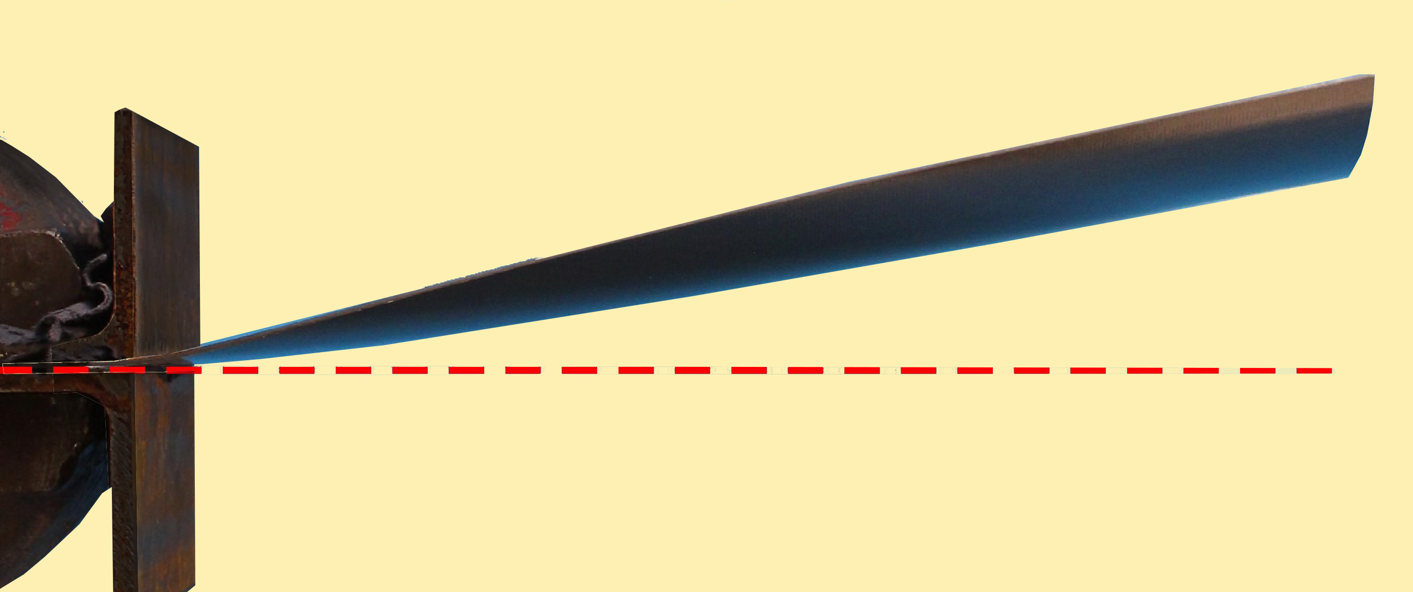
Although our theory is relevant in many circumstances, we confine the attention to a specific prototypical problem having several applications in the design of morphing structures, such as turbine blades or air inlets [21, 37, 40].
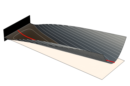
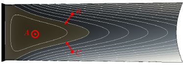
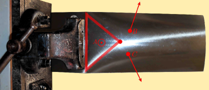
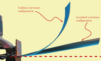
We consider a shell which in its initial stress-free natural configuration is cylindrical, shallow and has a rectangular planform, see Fig. 1. A portion of this shell, the one indicated by gray pattern in Fig. 1, is constrained to become flat after the application of a suitable clamp [7]. Clearly, this clamping produces a state of stress. For sufficiently shallow shells, bending is not uniform, as the curvature variation localizes near the clamped side, see for instance Fig. 2 (top) and the experimental and numerical results in [9]. Specifically, a small region is formed where the variation of Gaussian curvature –say – is localized. In Fig. 2 such a region corresponds to a neighbourhood of the point ; indeed, the normals to the shell surface in the three points , and identify a positive solid angle in the three-dimensional unit sphere, distintive mark of a positive Gaussian curvature. As the variation of Gaussian curvature implies the presence of membrane deformations, due to the Gauss Theorema Egregium, these regions are particularly interesting and were object of several studies, see for instance [12, 20].
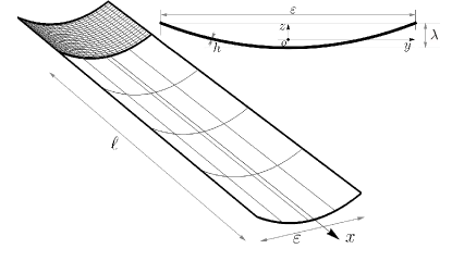
The relevant geometric parameters are sketched in Fig. 1; we call the shell planform, being the effective length of the part of the cantilever shell which does not undergo clamping and its width. Moreover, denotes the shell thickness and its curvature in the direction. The total deepness of the initial configuration, see Fig. 1, can be expressed in terms of curvature being . The four geometric parameters (, , and ) are required to satisfy
| (1) |
corresponding respectively to a thin, shallow shell whose planform resembles a rod-like body. As in the shallow regime the curvature scales as , we introduce the dimensionless parameter .
The parameter determines the initial stress-free curvature and, therefore, the level of stress after clamping; for our problem becomes trivial. With reference to the axes chosen in Fig. 1, we have
| (2) |
where is the unit vector in the direction and is the symmetric tensor defining the initial curvature. As the stress-free shape is cylindrical, its Gaussian curvature vanishes .
2 Dimensional reduction from the inextensible Koiter model
Before introducing the deduction from the FvK model, we begin with a dimensional reduction starting from the nonlinear model of Koiter’s inextensible shells (see, e.g., chapter 10 in [14], or [38]). The purpose is twofold: yielding some useful insights in a simpler context and obtaining a first one-dimensional theory that allows to determine analytical solutions, a circumstance that is not affordable for the extensible model; the generalization to the more general case will then result more terse. A shell is said to be inextensible when its membrane deformations vanish almost everywhere on . The physical justification for such model is found in the limit ; since the ratio between the membrane and bending stiffnesses scales as , the relative cost of membrane deformations becomes increasingly high and these deformations tend to localize over set with vanishing area, curves (creases) or points (d-cones). We refer to [39] for more details.
Within the inextensible hypothesis, the shell stable configurations are found solving the following constrained minimization problem of the bending energy:
| (3) |
where . The tensor fields represents the finite curvature, the stress-free finite curvature, and the constitutive tensor yields the bending stiffness. As it is known, the condition ensures the existence of a surface associated to the field . A classical approach, in order to satisfy this condition, is to seek solutions in the form
| (4) |
for some scalar field . We remark that, other than being a potential to generate a vanishing curl tensor field, the scalar field has no direct physical meaning. However, when the shell is shallow, as in our problem, the field can be interpreted as the transversal displacement field , (see [10]), as the finite curvature can be approximated by the infinitesimal curvature
| (5) |
Once substituted with in (3), the condition translates into . Hence, we use a simple Galerkin method to deduce a one-dimensional rod model, and then provide the following Ansazt for :
| (6) |
where the function , expressing the -dependence of the relevant fields in the problem, is given by
| (7) |
Remark 1
From (7) we have
| (8) |
where represents the -average value of the function . Using (6), one gets
| (9) |
Hence, for any cross-section of the shell, we can interpret as the displacement in the direction of its center of mass (point in Fig.1) and as the average of the dimensionless curvature in the -direction.
Remark 2
Clearly more complex Ansäzte can be used. An easy improvement could be to increase the polynomial order of to satisfy the boundary conditions for the bending moment, , along the sides . However, we are only interested in the simplest possible choice allowing for the description of the Gaussian curvature along the rod axis . The non-rigid micro-structure introduced using (6) is sufficient to our purposes.
Remark 3
Remark 4
The minimization problem (3) does not involve external forces, because in the problem at hand there are not. Considering them is not straightforward, but manageable. The proposed approach is in the spirit of the so-called intrinsic elasticity (see, e.g., [17]), for which the primary unknowns are the strain measures, instead of the displacement field, as in the classical approach. Adding forces within this framework requires to express the load potential in terms of strain — in our case in terms of ; to this purpose it is sufficient to have recourse to the Cesàro-Volterra formula (see, e.g., [16]). Once the displacement is expressed as a linear functional of the curvature field, the resulting minimization problem will contain an additional linear term in .
Using (4) and (6) we obtain the matrix field representing the approximated curvature, namely . In matrix form, it reads
| (10) |
where a prime indicates the derivative of a function with respect to its argument. When the functions and are varied in , spans a subspace of and, therefore, the reduced energy, namely , is finite. In particular, for isotropic materials, the reduced energy reads
| (11) |
where , with the bending stiffness in the -direction, being the Young modulus, the 2D Poisson ratio and the identity tensor.
As for the constraint in requiring a curvature with a vanishing determinant, the Gaussian curvature of (10) turns out to be
| (12) |
For to belong to almost everywhere in , the field must vanish: a trivial solution due to the fact that does not have sufficient degrees of freedom111More elaborate Ansätze with a finite number of terms would not help either.. However, aiming at approximate solutions in the limit , we require only its -average
| (13) |
to vanish almost everywhere in .
Finally, we formulate our first rod model as the following constrained minimization problem
| (14) |
where . Being derived by (3), this model will be referred in the following as the inextensible rod model.
3 Dimensional reduction from the Föppl–von Kármán shell model
We discuss the derivation of a rod model starting from the assumption of a thin shallow shell satisfying the Föppl–von Kármán equations. With respect to the previous section, the shell can undergo membrane deformations despite the fact that their cost (=stiffness) scales as , whilst the cost of bending deformations, scaling as , is sensibly smaller for thin shells.
If an initially curved shape of is considered, the model is often referred as Marguerre–von Kármán’s [ciarletgMvK]. For isotropic materials, it consists in finding the pair such that
| (15) | |||
| (16) |
where, for two given scalar fields and , denotes the Monge-Ampère crochet222Specifically, in Cartesian coordinates we have ., and is the Laplacian operator.
The fields and represent the displacements in the -direction of the shell points in the current and stress-free configurations with respect to the flat reference configuration. As we have already discussed, in the limit of shallow shells, their second gradient gives the curvatures fields and for .
The field is the Airy stress function. With respect to the case of inextensible shells, is the additional field allowing to account for membrane stress and membrane deformations, respectively
| (17) |
and to define the membrane energy
| (18) |
where is the membrane stiffness. For more details on the derivation and meaning of the FvK equations we refer the interested reader to [3]. In addition, we notice that general boundary conditions for the problem (15)–(16) are treated in several papers (see [5, ciarletgMvK]); in the following, we will consider only the special case corresponding to our problem.
In [5, 6] we have shown that eqs. (15)-(16) can be deduced by enforcing the following mixed variational problem:
| (19) |
where and are two suitable subsets of and the functional is given by the splitting:
| (20) |
In particular, for the case under consideration the Airy function is required to vanish on , so that .
Let us remark that both the bending and the membrane energy are quadratic and convex with respect to and . Last addend in (20) is the only term introducing non-linearities; it does not have have any constitutive character but couples the fields and , i.e., the bending and membrane problems.
Dimensional reduction is achieved, once again, via the Galerkin method. In other words, we seek solutions for and in the form
| (21) |
with and given functions of the -coordinate, see (7) and (24) respectively. The extensible rod model is equivalent to the solution of the reduced min-max problem
| (22) |
with the reduced action functional. The condition follows easily once noted that vanishes on the lateral boundaries (see (23) below).
Specifically, we have used for the same Ansatz of the inextensible case, namely (6) with as in (7). For the function expressing the -dependance of the membrane fields, we choose the lowest-order polynomial satisfying
| (23) |
i.e.
| (24) |
Using (17)1 and (21)2, this choice suffices to describe all the components of the membrane stress tensor:
| (25) |
Moreover conditions (23) allow to satisfy the boundary conditions and along the lateral sides of the shell.
For the reduced functional, in the case of isotropic materials, we obtain
| (26) |
where is the reduced bending energy already computed in (11) and
| (27) |
is the reduced membrane energy.
Remark 5
Since , the mean value of on the cross-section, i.e. the axial stress in the resulting rod, vanishes. This is not the case in the model developed in [30]. However, here the membrane stress is able to describe the zero-average stress distribution on the rod cross-section corresponding to a bending moment.
Remark 6
The Euler-Lagrange equation of with respect to gives
| (28) |
where is another one-dimensional approximation of the shell Gaussian curvature. Eq. (28) keeps track of the two-dimensional compatibility condition (16). Given , Eq. (28) in terms of is analog to the well known equation of a beam on an elastic ground à la Winkler (see, e.g., [43]); formally its solution can be expressed as the convolution integral
| (29) |
with is the Green function of the fourth-order differential operator .
Hence, the two-dimensional compatibility equation translates into a non-locality of the resulting rod model being formally equivalent to:
| (30) |
In particular, a root-finding calculation shows that the particular solutions of the differential operator decay as . This implies that a concentrated variation of the Gaussian curvature of the order decays to at distance . Thus, the effective radius of non-locality is of the order .
4 Results
In this section, we solve the problem presented in Sec. 1.1, by adopting both the inextensible and the extensible rod models; analytical results are possible just in the former case and this is why we examine it first. In particular, our interest is to describe the region of localized curvature shown in Fig. 2 estimating its width , and the extremal values of curvature therein and . For sake of simplicity, in this section, we limit the analysis to the isotropic case.
4.1 Analytical results: inextensible case
We must solve the minimization problem (14) with the reduced energy given in (11). Letting be the field of axial curvature and neglecting the term involving in (11) (see remark 7), we face the following problem:
| (31) |
with and constrained to satisfy .
Remark 7
The coefficients weighting and in (11) are respectively given by:
| (32) |
Since , the Poincaré-Wirtinger inequality holds true and:
| (33) |
Hence, we can estimate that , vanishing in the limit .
The problem (31) is equivalent to
| (34) |
with the conic surface
| (35) |
and , the points of coordinates:
| (36) |
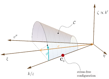
this latter corresponding to the stress-free configuration. Under the proposed change of coordinates, see [33], minimizing the bending energy under the inextensibility constraint is reformulated as the search of a sequence of points lying on the cone having minimal (total) distance from the target point (see Fig. 3).
It easily seen that the condition translates the inextensibility constraint or, in other words, the condition
| (37) |
for the cross-section average of the Gaussian curvature to vanish.
However, having this geometric understanding of the problem, it is clear that for a smooth parametrization of the inextensibility constraint, we need an angular coordinate. Specifically, we use the cone coordinates shown in Fig. 3: any point of the cone can be written in the form
| (38) |
for some choice of the angular anomaly and of the curvature333The coordinate is actually proportional to the mean curvature . . Of course, there is a correspondence between and , which has to been determined. For a given point , the compatibility constraint (37) reveals how , and have to be related in order to be admissible at that point. If we adopt the parametrization of the cone in terms of , we have to put in correspondence and with some auxiliary functions and . In other words, we need to find a correspondence between the physical point and the coordinates , in order to find the map . From a geometrical point of view, this means that the admissible configuration of a point of the rod may be visualized as a point over the cone ; a sequence of points (a curve) laying on the cone then represents the set of the admissible configurations of the whole rod. A way to minimize the bending energy, is to require that each point of such a curve has minimum distance from the point corresponding to the stress-free configuration. It is not difficult to see that
| (39) |
Moreover, the axial and transverse curvatures can be expressed as
| (40) |
respectively.
Requiring the distance (39) to be minimal with respect to implies
| (41) |
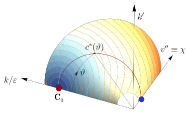
Fig. 3 (b) is instrumental to understand the geometrical meaning of the procedure we intend to adopt. For a fixed anomaly , we determine the optimal , i.e., the optimal value of the radial coordinate (or rather the mean curvature) in order to minimize the bending energy; then we need to determine the curve (red in Fig. 3 (b)) through , still lying over the cone, whose points locally minimize the distance from , representing the stress-free configuration. It is worth noticing that such a procedure requires the local minimization of the distance via (41). This is a condition sufficient, but not necessary, to minimize (30), i.e., the total distance to . Solutions minimizing the total distance without necessarily satisfying (41) in the whole domain could be possible, in principle.
On substituting (41) in (40), we get:
| (42) | ||||
At this point, if knew the map , we would be in position to obtain the solution of the problem, determining the unknowns and . This is our next goal.
The compatibility equation suggests the one-to-one mapping between the spatial variable and the angular variable on the cone which is the key to solve the problem. Indeed, from we obtain
| (43) |
valid for . Inserting (42) and integrating, we deduce
| (44) |
It is easily checked that, for and , is strictly negative and maps the set into monotonically with .
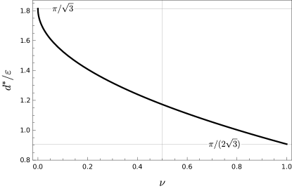
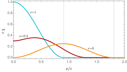
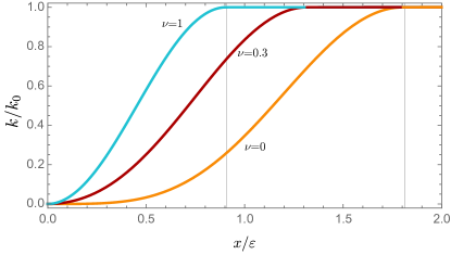
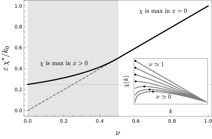
The inverse function of (44), say , allows to determine and from (42). This solution is valid until the point in Fig. 3 is reached for . Indeed, for the distance is minimized by remainining in the same point . Thus is actually the size of the region where the curvature localizes; the ratio is plotted against in Fig. 4. Unfortunately, the inverse function of (44) cannot be analytically determined for arbitrary values of ; however the problem of its numerical determination is well-posed since is strictly monotone. The solutions for the axial and transverse curvatures are plotted in Fig. 5 for some values of the Poisson ratio.
Although cannot be analytically determined, in general, closed forms of the maximal value of the axial curvature can be achieved. To this end, we eliminate from (42) and introduce the map
| (45) |
The maximum is attained for , solution of the stationarity condition , yielding
| (46) |
Here, we have used the fact that is a monotonically increasing positive function, whose codomain is . Finally, the maximum value of the axial curvature scales as being
| (47) |
which is plotted in Fig. 6 against positive Poisson ratios. It is easily seen that the axial curvature is always non negative; and therefore, the minimum value of the curvature is for any .
Remark 8
The solution found implies a localization of the axial rod curvature that tends to a Dirac delta distribution in the limit . Indeed, over a region , the integral
| (48) |
being finite and independent of .
4.2 Numerical results for the extensible cases
The solutions of the extensible rod are found as saddle points, see (22), of the functional given in (26). As a numerical procedure is necessary to this end, we use a standard finite element method. The domain is discretized into elements with a mesh suitably refined near the clamp . Since all the fields belongs to , we choose, for all of them, Langrange polynomials of order 3 ensuring the inter-element continuity of their values and their first derivatives. In every node of the mesh we have degrees of freedoms (total size of the problem scalar unknowns). Storing in the vector the degrees of freedom relative to and and in the vector the ones relative to , the action functional (26) is written as
| (49) |
with and positive definite second order tensors, and vectors and the third order tensor responsible for the coupling between membrane and bending problems. We compute once for all these tensors avoiding the reassembling of the stiffness matrices even if is a nonlinear problem. The saddle point satisfying (22) is found by iteratively finding the root of the following system:
| (50) |
Clearly, the system can have several solutions depending on the initial guess , cfr. section 5.1. To follow the equilibrium branch relative to the curvature localization shown in Fig. 2 suffices to start from , .
As a benchmark solution for our reduced rod models, we numerically solve the FvK shell equations with the boundary conditions provided by the problem at hand. To this aim we resort to the code provided by the FEniCS shells project [1, 31] which implements a standard displacement-based FE procedure (that is, the solution is found by minimizing the shell elastic energy). The domain has been discretized with both structured and unstructured meshes suitably refined near the clamp so that the mesh size is smaller than the shell thickness, while membrane locking is avoided by appropriately choosing the discrete spaces for in-plane and transverse displacements. More in detail, we used standard Lagrangian elements for both of them, weakly enforcing -continuity of the piecewise continuous transverse displacement by penalizing the jump of the normal component of its gradient through the element facets. We chose the penalty parameter to be of the order of the norm of the bending stiffness tensor.
4.3 Comparisons
We compare the results obtained by the FvK shell model, assumed as a benchmark, with the inextensible and extensible rod models derived in sections 2 and 3. In the numerical simulations we have chosen , and this last choice being irrelevant as far as . Indeed, the localization of curvature happens within a distance from the clamp and this is actually the only region where we have plotted the relevant fields. Results are independent of the Young modulus but do depend on the Poisson ratio.
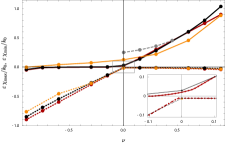
Figs. 7a and 7b plot the maximal and minimal axial curvature and the size of localization region as estimated by the three models under consideration for the admissible range of Poisson ratio . The inextensible rod model results are limited to the case : negative values of the Poisson ratio are in principle possible, but the geometric construction presented in 4.1 would require to consider the singular point corresponding to the vertex of the cone, an analytical obstacle that we exclude for sake of simplicity. We used a black color to label the benchmark FvK shell model, gray and dark-red curves to indicate the inextensible and extensible rod models, respectively. As a further benchmark, we performed a FE-based analysis with the fully non-linear Naghdi shell model [31] (orange curves); we conclude that all the relevant estimates are well captured by our theory. We see that the sup-norm of the curvature field is very well estimated by the simple formula
| (51) |
We recall, see (47), that this can be obtained as the point on the cone axis , having minimal distance form the stress-free configuration . The inset in Fig. 7b reveals that the maximum and minimum values of the curvature, considered as functions of , never intersect: thus, the axis is always bent, even close to . In general, we remark a good agreement of both the rod models with the two-dimensional results. In all three cases, the maximum of axial curvature scales as whilst the localization size scales as ; hence, the rod models are able to catch the macroscopic deformation of the rod, independently of the cross-section dimension . The inextensible model overestimates the maximal curvature for vanishing values of the Poisson ratio: in this case the interplay between axial and transverse curvature, already constrained by the inextensibility hypothesis, is further limited since the coupling terms and of the Voigt representation of vanish with .
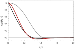
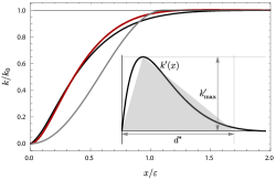
For , Figs. 8a and 8b plot the spatial distributions of the axial and transverse curvatures444For the FvK shell the axial and transverse curvatures are obtained from the displacement field through (9). within the localization region. While the extinction length for the inextensible case has been obtained in closed form in Sect. 4.1, both the curvatures of the FvK shell and of the extensible rod exponentially decay towards their asymptotic values and . For both these models the size of the localization region has been estimated approximating the area subtended to the graph of by a triangle having height , namely
| (52) |
as shown in the inset of Fig. 8b.
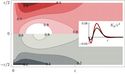
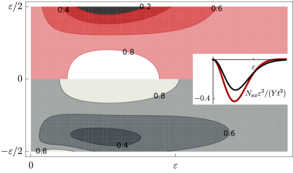
For the macroscopic behavior of the rod, the simple analytic expressions obtained by the inextensible model for , and in section 4.1 seem surprisingly accurate, cfr. Figs. 7a-7a. However, the inextensible model, derived from the constraint for to vanish almost everywhere in , could never describe neither the Gaussian curvature field nor the membrane stresses. To this aim, we compare the benchmark FvK results only with the extensible rod model. In Fig. 9 the level curves of the Gaussian curvature are plotted. These level curves are rescaled to range within and corresponding respectively to the minimum and maximum values attained by both the models in :
Being symmetric with respect to , we have used the upper part to draw, in red tones, as predicted by the extensible rod and the lower part to draw in gray tones the results of a two-dimensional FE analysis with FvK. In the same Figure, the inset plots the weighted average of the two-dimensional field of Gaussian curvature and the reduced notion of Gaussian curvature, given by the right-hand side of (13). These results are in very good agreement with of the FvK model.
From the knowledge of the fields and , Eq. (6) allows to reconstruct the two-dimensional displacement, and then the deformed surface.
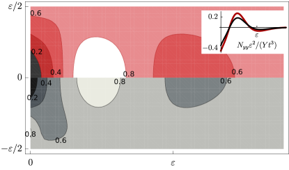
Finally, we remark that the extensible rod model allows for an estimate of the membrane stress fields via the scalar field . Specifically, through Eqns. (21) and (25) we reconstruct the two-dimensional fields of the stress and and compare them to the ones of the FvK shell model in Figs. 10a-10b. Again a remarkable agreement is apparent also for the membrane fields. Slight discrepancies are localized at the edges , where our Ansatz is not probably sufficient to catch the exact -distribution of the stress fields and more terms would be required.
5 Discussion and conclusions
We have presented two new models of thin-walled non-linear rods, whose main features are:
-
1.
The transversal section is not rigid. For this reason, an additional kinematical descriptor is introduced, accounting for the change in curvature of the transversal section. The resulting 1D model is then endowed with a 1D notion of Gaussian curvature, keeping track of the 2D character of the shell model from which we started.
-
2.
In standard dimensional reduction, starting from a two-dimensional model, the effects of the compatibility kind of evaporate. In both our theories, a compatibility condition coupling bending and membrane problems is deduced, endowing the model with a 2D character.
-
3.
Localization phenomena, such as d-cones, are captured by our models. Analytical estimates are possible in the inextensible case.
A key question may arise: is there any circumstance in which the role of the 1D compatibility equation (28) (or (37) for the inextensible case) is particularly undeniable?
If we confine the attention to the inextensible model, satisfying the compatibility translates into requesting that the solution belongs to the cone (35); the stress-free configuration (point in Fig. 3) belongs to ; the boundary conditions for compel the solution to tend to a point belonging to as well; all in all, this particular set of boundary conditions leads the solution to stay close to , even if no a priori constraint is taken into account.
One then might argue that the compatibility does not have a strong role, at least for this specific problem and minimizing the bending energy would suffice to obtain solutions sufficiently close to the cone. Nevertheless, regardless of the boundary conditions that activate or not the compatibility constraint, the nonlocal (or inextensible) and the pure bending model differ for a crucial point: the bending energy is a positive quadratic functional, and then its direct minimization delivers a unique solution; this is not the case when the model is endowed with the compatibility condition. Thus, multiple solutions are possible if the compatibility is taken into account, as we will see in the next subsection: besides localization phenomena, the 1D compatibility induces mutistability.
5.1 Compatibility and multistability: uniform curvature solution
For the inextensible case the compatibility requires the condition to hold. This introduces a strong nonlinearity in the problem to solve which we introduced the cone coordinates in Sect.4.1. We show below that one can indeed have multiple equilibria and, in some cases, multiple stable equilibria.
The evaluation of the optimal in (41) allows to obtain the bending energy on the cone as a function of
| (53) | ||||
This energy admits more than one stationarity point: together with the solution presented in Sec. 4.1, it is easy to see that has a stationarity point for , a solution corresponding to
| (54) |
Indeed for we have and therefore ; recalling the compatibility equation, (54) follows. This configuration corresponds to the point blue in Fig. 3 (b). Hence, we could have a second possible configuration of the rod where all points have the same constant axial curvature, being the transversal curvature null.
The stability of this configuration can be studied on evaluating the second derivative of with respect to at the point :
| (55) |
which is negative for .
Thus, the configuration (54) is not stable. We conclude that for an isotropic material, the only stable configuration is the localized one; however, removing the hypothesis of isotropy could lead to a different scenario. To see this, let us consider an orthotropic material; the stiffness tensor is given by the following Voigt representation:
| (56) |
with , , ; the constant represents the ratio between the two Young moduli and represents the shear modulus. Isotropic materials are obtained when .
The change of coordinates (36), to diagonalize the bending energy, has to be replaced by
| (57) |
The cone (35) of inextensible curvatures then becomes:
| (58) |
The cone has then an elliptical cross section, whose semi-axes are in fact and . The change of variable (38) then now reads:
| (59) |
which allows to determine the analytical expression for the bending energy of the orthotropic rod . As in Section 4.1, we first evaluate the value that makes stationary , and then deduce . We do not the details here but, again, is a point that renders stationary. Being and , this stationary point is stable if the component of the Hessian
| (60) |
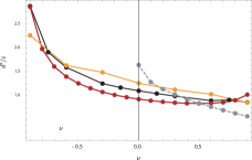
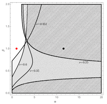
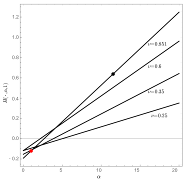
a function of the material parameters , and , is positive. The analytical expression of can be determined, but it is quite cumbersome and we do not report it. However, we plot, in Fig. 11a (a), the regions of the plane where for several values of the Poisson ratio. In these shaded regions, there are at least two stable configurations: not only the localized-curvature solution discussed in the previous sections but also equilibrium , corresponding to the configuration (54), is stable. In Fig. 11a (b) we plotted the cross section of for , which shows that there is not a sudden shift in the behavior, as those described within the framework of the catastrophe theory.
References
- Alnæs et al. [2015] Alnæs, M.S., Blechta, J., Hake, J., Johansson, A., Kehlet, B., Logg, A., Richardson, C., Ring, J., Rognes, M.E., Wells, G.N., The FeniCS Project Version 1.5, Archive of Numerical Software, 2015, 3.
- Audoly and Hutchinson [2016] Audoly, B., Hutchinson, J., Analysis of necking based on a one-dimensional model, Journal of the Mechanics and Physics of Solids, 2016, 97, 68–91.
- [3] Audoly, B., Pomeau, Y., Elasticity and Geometry, Oxford University Press, 2010.
- [4] Ballard, P., Miara, B., Formal asymptotic analysis of elastic beams and thin-walled beams: A derivation of the Vlassov equations and their generalization to the anisotropic heterogeneous case, 2018, 12, 1547.
- Brunetti et al. [2019a] Brunetti, M., Favata, A., Paolone, A., Vidoli, S., A mixed variational principle for the Föppl–von Kármán equations, Applied Mathematical Modelling, 2019a, 79, 381-391.
- Brunetti et al. [2019b] Brunetti, M., Favata, A., Vidoli, S., A low-order mixed variational principle for the generalized Marguerre–Föppl–von Kármán equations, Meccanica, 2019b, 1-8.
- [7] Brunetti, M., Vincenti A., Vidoli, S. A class of morphing shell structures satisfying clamped boundary conditions, International Journal of Solids and Structures, 82, 47–55, 2016.
- [8] Brunetti, M., Vidoli, S., Vincenti, A., Bistability of orthotropic shells with clamped boundary conditions: An analysis by the polar method, Composite Structures, 194, 388–397, 2018.
- Brunetti et al. [2018] Brunetti, M., Kloda, L., Romeo, F., Warminski, J., Multistable cantilever shells: analytical prediction, numerical simulation and experimental validation, Composites Science and Technology, 2018, 165, 397–410.
- Calladine [1983] Calladine, C.R., Theory of Shell Structures, Cambridge University Press, 1983.
- Calladine and Seffen [2019] Calladine, C.R., Seffen, K.A., Folding the Carpenter’s Tape: Boundary Layer Effects, Journal of Applied Mechanics, 2019, 87.
- Cerda and Mahadevan [1998] Cerda, E., Mahadevan, L., Conical surfaces and crescent singularities in crumpled sheets, Physical Review Letters, 1998, 80, 2358–2361.
- [13] Ciarlet, P., Mathematical Elasticity. Volume II: Theory of Plates, North-Holland, 1997.
- [14] Ciarlet, P. Mathematical Elasticity, Vol III Theory of Shells, North Holland, 2000.
- [15] Ciarlet, P., A justification of the von Kármán equations, Archive for Rational Mechanics and Analysis, 1980, 73, 349-389.
- [16] Ciarlet, P., Gratie, L., Serpilli, M., Cesàro-Volterra path integral formula on a surface, Mathematical Models and Methods in Applied Sciences, 2009, 19 (03), 419-441.
- [17] Ciarlet, P., Mardare, C., The intrinsic theory of linearly elastic plate, Mathematics and Mechanics of Solids, 2019, 24, 1182-1203.
- Cimetière et al. [1988] Cimetière, A., Geymonat, G., Le Dret, H., Raoult, A., Tutek, Z., Asymptotic theory and analysis for displacements and stress distribution in nonlinear elastic straight slender rods, Journal of Elasticity, 1988, 19 111-161.
- Coleman and Newman [1988] Coleman, B., Newman, D., On the rheology of cold drawing. i. elastic materials, Journal of Polymer Science Part B: Polymer Physics, 1988, 26, 1801-1822.
- Conti and Maggi [2008] Conti, S., Maggi, F., Confining thin elastic sheets and folding paper, Archive for Rational Mechanics and Analysis, 2008, 187, 1–48.
- [21] Daynes, S., Weaver, P.M., Potter, K.D., Aeroelastic study of bistable composite airfoils, Journal of aircraft, 2009, 46, 6, 2169–2174.
- Davini et al. [2014a] Davini, C., Freddi, L., Paroni, R., Linear models for composite thin-walled beams by -convergence. Part I: Open cross sections, SIAM Journal on Mathematical Analysis, 2014a, 46, 3296-3331.
- Davini et al. [2014b] Davini, C., Freddi, L., Paroni, R., Linear models for composite thin-walled beams by -convergence. Part II: Closed cross-sections, SIAM Journal on Mathematical Analysis, 2014b, 46, 3332–3360.
- [24] Föppl, A., Vorlesungen über technische Mechanik, BG Teubner, 1909, 6.
- Freddi et al. [2016b] Freddi, L., Hornung, P., Mora, M., Paroni, R., A variational model for anisotropic and naturally twisted ribbons, SIAM Journal on Mathematical Analysis, 2016b, 48, 3883-3906.
- Freddi et al. [2018] Freddi, L., Hornung, P., Mora, M., Paroni, R., One-dimensional von Kármán models for elastic ribbons, Meccanica, 2018, 53, 659-670.
- Freddi et al. [2012] Freddi, L., Mora, M., Paroni, R., Nonlinear thin-walled beams with a rectangular cross-section – Part I, Mathematical Models and Methods in Applied Sciences, 2012, 22.
- Freddi et al. [2013] Freddi, L., Mora, M., Paroni, R., Nonlinear thin-walled beams with a rectangular cross-section – Part II, Mathematical Models and Methods in Applied Sciences, 2013, 23, 743-775.
- Geymonat et al. [2018] Geymonat, G., Krasucki, F., Serpilli, M., Asymptotic derivation of a linear plate model for soft ferromagnetic materials, Chinese Annals of Mathematics. Series B, 2018, 39, 451–460.
- Guinot et al. [2012] Guinot, F., Bourgeois, S., Cochelin, B., Blanchard, L., A planar rod model with flexible thin-walled cross-sections, International Journal of Solids and Structures, 2012, 49, 73-86.
- Hale et al. [2018] Hale, J.S., Brunetti, M., Bordas, S.P.A., Maurini, C., Simple and extensible plate and shell finite element models through automatic code generation tools, Computers and Structures, 2018, 209, 163–181.
- Hamdouni and Millet [2006] Hamdouni, A., Millet, O., An asymptotic non-linear model for thin-walled rods with strongly curved open cross-section, International Journal of Non-Linear Mechanics, 2006, 41, 396-416.
- Hamouche et al. [2017] Hamouche, W., Maurini, C., Vidoli, S., Vincenti, A., Multi-parameter actuation of a neutrally stable shell: a flexible gear-less motor, Proceedings of the Royal Society A: Mathematical, Physical and Engineering Sciences, 2017, 473, 20170364.
- Lestringant and Audoly [2017] Lestringant, C., Audoly, B., Elastic rods with incompatible strain: Macroscopic versus microscopic buckling, Journal of the Mechanics and Physics of Solids, 2017, 103, 40-71.
- Lestringant and Audoly [2018] Lestringant, C., Audoly, B., A diffuse interface model for the analysis of propagating bulges in cylindrical balloons, Proceedings of the Royal Society A: Mathematical, Physical and Engineering Sciences, 2018, 474.
- Lestringant and Audoly [2019] Lestringant, C., Audoly, B., Asymptotically exact strain-gradient models for nonlinear slender elastic structures: A systematic derivation method, Journal of the Mechanics and Physics of Solids, 2019, 136.
- [37] Mattioni, F., Weaver, P.M., Friswell, M.I., Multistable composite plates with piecewise variation of lay-up in the planform, International Journal of Solids and Structures, 2009, 46, 1, 151-164.
- [38] Lods, V., Miara, B., Nonlinearly Elastic Shell Models: A Formal Asymptotic Approach II. The Flexural Model, Archive for Rational Mechanics and Analysis volume 142, 355–374(1998).
- Müller and Olbermann [2014] Müller, S., Olbermann, H., Conical singularities in thin elastic sheets, Calculus of Variations, 2014, 49, 1177-1186.
- [40] Panesar, A.S., Weaver, P.M., Optimisation of blended bistable laminates for a morphing flap, Composite Structures, 2012, 94, 10, 3092-3105
- Sadowsky [1930] Sadowsky, M., Ein elementarer Beweis für die Exis-tenz eines abwickelbaren Möbiuschen Bandes und die Zurückführung des geometrischen Problems auf ein Variationsproblem, Sitzungsber. Preuss. Akad. Wiss., 1930.
- Sanchez-Hubert and Sanchez Palencia [1999] Sanchez-Hubert, J., Sanchez-Palencia, E., Statics of curved rods on account of torsion and flexion, European Journal of Mechanics, A/Solids, 1999, 18, 365-390.
- [43] Timoshenko, S., Strength of materials: Part II, CBS Publishers & Distributors, 1956.
- [44] von Kármán, T., Festigkeitsprobleme im maschinenbau, Springer, 1907, 311-385.
- Wunderlich [1962] Wunderlich, W., Über ein abwickelbares Möbiusband, Monatshefte für Mathematik, 1962, 66, 276-289.