Dynamic thin-shell black-bounce traversable wormholes

Abstract

Based on the recently introduced black-bounce spacetimes, we shall consider the construction of the related spherically symmetric thin-shell traversable wormholes within the context of standard general relativity. All of the really unusual physics is encoded in one simple parameter $a$ which characterizes the scale of the bounce. Keeping the discussion as close as possible to standard general relativity is the theorist’s version of only adjusting one feature of the model at a time. We shall modify the standard thin-shell traversable wormhole construction, each bulk region now being a black-bounce spacetime, and with the physics of the thin shell being (as much as possible) derivable from the Einstein equations. Furthermore, we shall apply a dynamical analysis to the throat by considering linearized radial perturbations around static solutions, and demonstrate that the stability of the wormhole is equivalent to choosing suitable properties for the exotic material residing on the wormhole throat. The construction is sufficiently novel to be interesting, and sufficiently straightforward to be tractable.

Keywords: black bounce; Lorentzian wormhole; traversable wormhole; thin shell.

I Introduction

One can tentatively trace back wormhole physics to Flamm’s work in 1916 Flamm and to the “Einstein-Rosen bridge” wormhole-type solutions considered by Einstein and Rosen (ER), in 1935 Einstein-Rosen . However, the field lay dormant for approximately two decades until 1955, when John Wheeler became interested in topological issues in general relativity geons . He considered multiply-connected spacetimes, where two widely separated regions were connected by a tunnel-like gravitational-electromagnetic entity, which he denoted as a “geon”. These were hypothetical solutions to the coupled Einstein-Maxwell field equations. Subsequently, isolated pieces of work do appear, such as the Homer Ellis’ drainhole concept homerellis ; homerellis2 , Bronnikov’s tunnel-like solutions bronikovWH , and Clement’s five-dimensional axisymmetric regular multiwormhole solutions Clement:1983tu , until the full-fledged renaissance of wormhole physics in 1988, through the seminal paper by Morris and Thorne Morris .

In fact, the modern incarnation of Lorentzian wormholes (and specifically traversable wormholes) now has over 30 years of history. Early work dates from the late 1980s Morris ; Yurtsever ; Visser:surgical ; Visser:examples ; Visser:1989a ; Visser:1989b ; Visser:1989c . Lorentzian wormholes became considerably more mainstream in the 1990s Visser:1990 ; Hochberg:1990 ; Frolov:1990 ; Visser:1990-PRD ; Visser:1990-mpla ; Visser:1992 ; Visser:1993 ; natural ; Kar1 ; Kar2 ; Poisson ; Visser:book ; gr-qc/9704082 ; gr-qc/9710001 ; Visser:1996 ; Teo:1998 ; hochvisserPRL98 ; hochvisserPRD98 ; gr-qc/9901020 ; Hochberg:1998 ; gr-qc/9908029 , including work on energy condition violations gvp1 ; gvp2 ; gvp3 ; gvp4 ; gvp:jerusalem ; Visser:cosmo99 ; Martin-Moruno:2017 , with significant work continuing into the decades 2000-2009 Barcelo:2000 ; gr-qc/0003025 ; Dadhich:2001 ; gr-qc/0205066 ; VKD ; gr-qc/0405103 ; gr-qc/0406083 ; Arellano:2006 ; Lobo:2007 ; Lobo-Nova ; Boehmer:2007rm ; Boehmer:2007md ; modgravity1 ; modgravity2 and 2010-2019 modgravity3 ; modgravity4 ; Bohmer:2011 ; Montelongo-Garcia:2011 ; Lobo:2012 ; Harko:2013 ; Mehdizadeh:2015jra ; Zangeneh:2015jda ; Lobo:2015 ; Boonserm:2018 ; Simpson:2018 ; Simpson:2019 ; Lobo:2017oab ; Rosa:2018jwp . We shall particularly focus on the thin-shell formalism Sen ; Lanczos ; Darmois ; Synge ; Lichnerowicz ; Israel , first applied to Lorentzian wormholes in Visser:surgical ; Visser:examples , and subsequently further developed in that and other closely related settings by many other authors Eiroa ; Lobo-Crawford ; FHK ; BLP ; Goncalves ; LLQ ; Lobo-ec-dust ; Lobo-CQG ; LL-PRD ; Sushkov ; Lobo-phantom ; Lobo-Crawford-2 ; Lobo-phantom2 ; Eiroa:cylindrical ; Eiroa:dilaton ; Eiroa:gauss-bonnet ; Rahaman1 ; Rahaman2 ; Eiroa:cosmic-strings ; Eiroa:gas ; Lemos:plane ; Eiroa:brans ; Eiroa:generalized-gas ; Eiroa:stability ; Eiroa:cylindrical2 ; Halisoy ; Dias ; Yue-Gao ; Lobo:phantom-stars ; Lake1 ; Lake2 . Our notation will largely follow that of Hawking and Ellis hawking-ellis . For the purposes of this article we will focus primarily on applying the technical machinery built up regarding spherically-symmetric thin-shell spacetimes in references Visser:surgical ; Visser:book ; Montelongo-Garcia:2011 ; Lobo:2012 ; Lobo:2015 , and for the bulk spacetimes (away from the thin shell) shall restrict attention to the recently developed black-bounce spacetimes of references Simpson:2018 ; Simpson:2019 (for related work, we refer the reader to Bronnikov:2006fu ; Bronnikov:2003gx ).

Consider the following candidate regular black hole (a black bounce) specified by the spacetime line element:

$$ds^{2}=-\left(1-\frac{2m}{\sqrt{u^{2}+a^{2}}}\right)dt^{2}+\left(1-\frac{2m}{\sqrt{u^{2}+a^{2}}}\right)^{-1}\,du^{2}+\left(u^{2}+a^{2}\right)\,d\Omega^{2}\,.$$ (1)

Here the $u$ and $t$ coordinates have the domains $u\in(-\infty,+\infty)$ and $t\in(-\infty,+\infty)$. In the original references Simpson:2018 ; Simpson:2019 the $u$ coordinate was called $r$, however we now want to use the symbol $r$ for other purposes. In this work, we shall analyse thin-shell constructions based on this spacetime. By considering the coordinate transformation $r^{2}=u^{2}+a^{2}$, we shall use the following completely equivalent line element:

$$ds^{2}=-\left(1-\frac{2m}{r}\right)dt^{2}+\left(1-\frac{2m}{r}\right)^{-1}\left(1-\frac{a^{2}}{r^{2}}\right)^{-1}\,dr^{2}+r^{2}\,d\Omega^{2}\,.$$ (2)

Here the $r$ coordinate is now a double-cover of the $u$ coordinate. It has the domain $r\in(a,+\infty)$, and can be interpreted as the Schwarzschild area coordinate — all the 2-spheres of constant $r$ have area $A(r)=4\pi r^{2}$. This choice has the additional advantage of making it easy to directly compare the current analysis with most other work in the literature. The $t$ coordinate has the usual domain $t\in(-\infty,+\infty)$. All of these black-bounce spacetimes are simple one-parameter modifications of Schwarzschild spacetime; for detailed analyses of the properties of these black-bounce spacetimes see references Simpson:2018 ; Simpson:2019 .

While Lorentzian wormholes are in general very different from Mazur–Mottola gravastars Mazur:2001 ; Mazur:2003 ; Mazur:2004a ; Mazur:2004b ; gravastar1 ; gravastar2 ; Lobo-gravastar1 ; Lobo-gravastar2 , it is worth pointing out that in the thin-shell approximation there are very many technical similarities — quite often a thin-shell wormhole calculation can be modified to provide a thin-shell gravastar calculation at the cost of flipping a few strategic minus signs Martin-Moruno:2011 ; Lobo:2015-novel-gravastar .

Structurally we organize the article as follows: We first introduce and briefly summarize the appropriate variant of the thin-shell formalism in Section II. Section III discusses some specific examples and applications. Finally we conclude in Section IV.

II Thin-shell formalism

We shall first perform a general (and relatively straightforward) theoretical analysis, somewhat along the lines laid out in reference Montelongo-Garcia:2011 , but with appropriate specializations, simplifications, and modifications. Subsequently we shall investigate a number of specific examples in the way of special cases and toy models. We discuss the bulk spacetimes in subsection II.1, the extrinsic curvature of the thin shells in subsection II.2, before moving on to the Lanczos equations in subsection II.3. We then discuss the Gauss and Codazzi equations in subsection II.4, before considering the equation of motion and its linearization in subsections II.5 and II.6. Finally we develop the master equation in subsection II.7, before moving on to the next section III where we shall discuss some specific examples and applications.

II.1 Bulk spacetimes

We initiate the discussion by considering two distinct “bulk” spacetime manifolds, ${\cal M_{+}}$ and ${\cal M_{-}}$, equipped with boundaries $\partial{\cal M_{+}}=\Sigma_{+}$ and $\partial{\cal M_{-}}=\Sigma_{-}$. As long as the boundaries are isometric, $\Sigma_{+}\sim\Sigma_{-}$, then we can define a manifold ${\cal M}={\cal M_{+}}\cup{\cal M_{-}}$, which is smooth except possibly for a thin-shell transition layer at $\Sigma_{+}\sim\Sigma_{-}$. In particular, consider two static spherically symmetric black-bounce spacetimes given on ${\cal M_{\pm}}$ by the following two-parameter $(m,a)$ Lorentzian-signature line elements $g_{\mu\nu}^{+}(x^{\mu}_{+})$ and $g_{\mu\nu}^{-}(x^{\mu}_{-})$:

$$ds^{2}=-\left(1-\frac{2m_{\pm}}{r_{\pm}}\right)dt_{\pm}^{2}+\left(1-\frac{2m_{\pm}}{r_{\pm}}\right)^{-1}\left(1-\frac{a_{\pm}^{2}}{r_{\pm}^{2}}\right)^{-1}\,dr_{\pm}^{2}+r_{\pm}^{2}\,d\Omega_{\pm}^{2}\,.$$ (3)

The usual Einstein field equations, $G_{{\mu}{\nu}}=8\pi\,T_{{\mu}{\nu}}$ (with $c=G=1$), imply that the physically relevant orthonormal components of the stress-energy tensor are (in the two bulk regions) specified by:

$$\rho(r) = -\frac{1}{8\pi}\frac{a^{2}\left(r-4m\right)}{r^{5}},$$ (4)

$$p_{r}(r) = -\frac{1}{8\pi}\frac{a^{2}}{r^{4}},$$ (5)

$$p_{t}(r) = \frac{1}{8\pi}\frac{a^{2}\left(r-m\right)}{r^{5}}\,.$$ (6)

Here $\rho(r)$ is the energy density, $p_{r}(r)$ is the radial pressure, and $p_{t}(r)$ is the transverse pressure. Given the spherical symmetry, $p_{t}(r)$ is the pressure measured in the two directions orthogonal to the radial direction. The subscripts $\pm$ (on $m_{\pm}$ and $a_{\pm}$) have been (temporarily) suppressed for clarity.

The null energy condition (NEC) is satisfied provided, for any arbitrary null vector $k^{a}$, the stress-energy $T_{\mu\nu}$ satisfies $T_{\mu\nu}\,k^{\mu}\,k^{\nu}\geq 0$. The radial null vector is $k^{\hat{\mu}}=(1,\pm 1,0,0)$ in the orthonormal frame where the stress energy is $T_{\hat{\mu}\hat{\nu}}={\rm diag}[\rho(r),p_{r}(r),p_{t}(r),p_{t}(r)]$. Then

$$(T_{\hat{\mu}\hat{\nu}}\,k^{\hat{\mu}}\,k^{\hat{\nu}})_{\mathrm{radial}}=\rho(r)+p_{r}(r)=-\frac{a^{2}(r-2m)}{4\pi r^{5}}<0.$$ (7)

To verify the negativity of this quantity, note that the bulk spacetime models a regular black hole when $a\in(0,2m)$, with horizons at $u_{H}=\pm\sqrt{(2m)^{2}-a^{2}}$, corresponding to $r_{H}=u_{H}^{2}+a^{2}=2m$. We therefore ‘chop’ the spacetime outside any horizons that are present. Hence in both of the bulk regions we have the condition that $r>2m$. Thus the radial NEC will be manifestly violated in both of the bulk regions of the black-bounce thin-shell spacetime. In the context of static spherical symmetry, this is sufficient to conclude that all of the standard energy conditions associated with general relativistic analysis will be similarly violated.

In the transverse directions we can choose the null vector to be $k^{\hat{\mu}}=(1,0,\cos\zeta,\sin\zeta)$ and so

$$(T_{\hat{\mu}\hat{\nu}}\,k^{\hat{\mu}}\,k^{\hat{\nu}})_{\mathrm{transverse}}=\rho(r)+p_{t}(r)=\frac{3a^{2}m}{8\pi r^{5}}>0.$$ (8)

While this is manifestly positive this is not enough to override the NEC violations coming from the radial direction.

II.2 Normal 4-vector and extrinsic curvature

The two bulk manifolds, ${\cal M_{+}}$ and ${\cal M_{-}}$, are bounded by the hypersurfaces $\partial{\cal M_{+}}=\Sigma_{+}$ and ${\cal M_{-}}=\Sigma_{-}$. These two hypersurfaces possess induced 3-metrics $g_{ij}^{+}$ and $g_{ij}^{-}$, respectively. The $\Sigma_{\pm}$ are chosen to be isometric. (In terms of the intrinsic coordinates, $g_{ij}^{\pm}(\xi)=g_{ij}(\xi)$, with $\xi^{i}=(\tau,\theta,\phi)$.) Thence a single manifold ${\cal M}$ is obtained by gluing together ${\cal M_{+}}$ and ${\cal M_{-}}$ at their boundaries, that is ${\cal M}={\cal M_{+}}\cup{\cal M_{-}}$, with the natural identification of the two boundaries $\Sigma_{\pm}=\Sigma$.

The boundary manifold $\Sigma$ possesses three tangent basis vectors ${\bf e}_{(i)}=\partial/\partial\xi^{i}$, with the holonomic components $e^{\mu}_{(i)}|_{\pm}=\partial x_{\pm}^{\mu}/\partial\xi^{i}$. This basis specifies the induced metric via the scalar product $g_{ij}={\bf e}_{(i)}\cdot{\bf e}_{(j)}=g_{\mu\nu}e^{\mu}_{(i)}e^{\nu}_{(j)}|_{\pm}$. Finally, in explicit coordinates, the intrinsic metric to $\Sigma$ is given by

$$ds^{2}_{\Sigma}=-d\tau^{2}+R^{2}(\tau)\,(d\theta^{2}+\sin^{2}{\theta}\,d\phi^{2}).$$ (9)

That is, the manifold ${\cal M}$ is obtained by gluing ${\cal M_{+}}$ and ${\cal M_{-}}$ at the 3-surface $x^{\mu}(\tau,\theta,\phi)=(t(\tau),R(\tau),\theta,\phi)$. The respective $4$-velocities, tangent to the junction surface and orthogonal to the slices of spherical symmetry, are defined on the two sides of the junction surface. They are explicitly given by

$$U^{\mu}_{\pm}=\left(\frac{\sqrt{\left(1-\frac{2m_{\pm}}{R}\right)\left(1-\frac{a_{\pm}^{2}}{R^{2}}\right)+\dot{R}^{2}}}{\left(1-\frac{2m_{\pm}}{R}\right)\left(1-\frac{a_{\pm}^{2}}{R^{2}}\right)^{1/2}},\;\dot{R},0,0\right).$$ (10)

Here $\tau$ is the proper time of an observer comoving with $\Sigma$, and the overdot denotes a derivative with respect to this proper time. Furthermore, the timelike junction surface $\Sigma$ is given by the parametric equation $f(x^{\mu}(\xi^{i}))=r-a(\tau)=0$, and the unit normal $4$-vector, $n^{\mu}$, is defined as

$$n_{\mu}={\nabla_{a}f\over||\nabla f||}=\pm\,\left|g^{\alpha\beta}\,\frac{\partial f}{\partial x^{\alpha}}\,\frac{\partial f}{\partial x^{\beta}}\right|^{-1/2}\;\frac{\partial f}{\partial x^{\mu}}\,.$$ (11)

Hence $n_{\mu}\,n^{\mu}=+1$ and $n_{\mu}e^{\mu}_{(i)}=0$. In the usual Israel formalism one chooses the normals to point from ${\cal M_{-}}$ to ${\cal M_{+}}$ Israel , so that the unit normals to the junction surface are provided by the following expressions:

$$n^{\mu}_{\pm}=\pm\left(\frac{\dot{R}}{\left(1-\frac{2m_{\pm}}{R}\right)\left(1-\frac{a_{\pm}^{2}}{R^{2}}\right)^{1/2}},\sqrt{\left(1-\frac{2m_{\pm}}{R}\right)\left(1-\frac{a_{\pm}^{2}}{R^{2}}\right)+\dot{R}^{2}},0,0\right)\,.$$ (12)

Taking into account spherical symmetry one may also obtain the above expressions from consideration of the contractions $U^{\mu}n_{\mu}=0$ and $n^{\mu}n_{\mu}=+1$. The extrinsic curvature, or second fundamental form, is typically defined as $K_{ij}=n_{{(}\mu;\nu{)}}e^{\mu}_{(i)}e^{\nu}_{(j)}$. Now, by differentiating $n_{\mu}e^{\mu}_{(i)}=0$ with respect to $\xi^{j}$, one obtains the following useful relation

$$n_{\mu}\frac{\partial^{2}x^{\mu}}{\partial\xi^{i}\,\partial\xi^{j}}=-n_{\mu,\nu}\,\frac{\partial x^{\mu}}{\partial\xi^{i}}\frac{\partial x^{\nu}}{\partial\xi^{j}},$$ (13)

so that the extrinsic curvature $K_{ij}$ can therefore be represented in the form

$$K_{ij}^{\pm}=-n_{\mu}\left(\frac{\partial^{2}x^{\mu}}{\partial\xi^{i}\,\partial\xi^{j}}+\Gamma^{\mu\pm}_{\;\;\alpha\beta}\;\frac{\partial x^{\alpha}}{\partial\xi^{i}}\,\frac{\partial x^{\beta}}{\partial\xi^{j}}\right)\,.$$ (14)

Finally, using both spherical symmetry and equation (14), the non-trivial components of the extrinsic curvature are given by:

$$K^{\theta\;\pm}_{\;\;\theta} = \pm\frac{1}{R}\,\sqrt{\left(1-\frac{2m_{\pm}}{R}\right)\left(1-\frac{a_{\pm}^{2}}{R^{2}}\right)+\dot{R}^{2}}\;,$$ (15)

$$K^{\tau\;\pm}_{\;\;\tau} = \pm\,\left[\frac{\ddot{R}-\frac{a_{\pm}^{2}}{R\left(R^{2}-a_{\pm}^{2}\right)}\dot{R^{2}}+\frac{m_{\pm}\left(R^{2}-a_{\pm}^{2}\right)}{R^{4}}}{\sqrt{\left(1-\frac{2m_{\pm}}{R}\right)\left(1-\frac{a_{\pm}^{2}}{R^{2}}\right)+\dot{R}^{2}}}\right]\,.$$ (16)

II.3 Lanczos equations and surface stress-energy

For the case of a thin shell, the extrinsic curvature need not be continuous across $\Sigma$. For notational clarity we denote the discontinuity in $K_{ij}$ as $\kappa_{ij}=K_{ij}^{+}-K_{ij}^{-}$. The Einstein equations, when applied to the hypersurface joining the bulk spacetimes, now yield the Lanczos equations:

$$S^{i}_{\;j}=-\frac{1}{8\pi}\,(\kappa^{i}_{\;j}-\delta^{i}_{\;j}\;\kappa^{k}_{\;k})\,,$$ (17)

where $S^{i}_{\;j}$ is the surface stress-energy tensor on the junction interface $\Sigma$. Due to spherical symmetry $\kappa^{i}_{\;j}={\rm diag}\left(\kappa^{\tau}_{\;\tau},\kappa^{\theta}_{\;\theta},\kappa^{\theta}_{\;\theta}\right)$, the surface stress-energy tensor reduces to $S^{i}_{\;j}={\rm diag}(-\sigma,{\cal P},{\cal P})$, where $\sigma$ is the surface energy density, and ${\cal P}$ the surface pressure. The Lanczos equations imply

$$\sigma = -\frac{1}{4\pi}\,\kappa^{\theta}_{\;\theta}\,,$$ (18)

$${\cal P} = \frac{1}{8\pi}(\kappa^{\tau}_{\;\tau}+\kappa^{\theta}_{\;\theta})\,.$$ (19)

Using the computed extrinsic curvatures (15)–(16), we now evaluate the surface stresses:

$$\sigma = -\frac{1}{4\pi R}\left[\sqrt{\left(1-\frac{2m_{+}}{R}\right)\left(1-\frac{a_{+}^{2}}{R^{2}}\right)+\dot{R}^{2}}+\sqrt{\left(1-\frac{2m_{-}}{R}\right)\left(1-\frac{a_{-}^{2}}{R^{2}}\right)+\dot{R}^{2}}\right],$$ (20)

$${\cal P} = \frac{1}{8\pi R}\left[\frac{1+\dot{R}^{2}\left(\frac{R^{2}-2a_{+}^{2}}{R^{2}-a_{+}^{2}}\right)+R\ddot{R}-\frac{m_{+}R^{2}+a_{+}^{2}\left(R-m_{+}\right)}{R^{3}}}{\sqrt{\left(1-\frac{2m_{+}}{R}\right)\left(1-\frac{a_{+}^{2}}{R^{2}}\right)+\dot{R}^{2}}}+\frac{1+\dot{R}^{2}\left(\frac{R^{2}-2a_{-}^{2}}{R^{2}-a_{-}^{2}}\right)+R\ddot{R}-\frac{m_{-}R^{2}+a_{-}^{2}\left(R-m_{-}\right)}{R^{3}}}{\sqrt{\left(1-\frac{2m_{-}}{R}\right)\left(1-\frac{a_{-}^{2}}{R^{2}}\right)+\dot{R}^{2}}}\right].$$ (21)

The surface mass of the thin shell is defined by $m_{s}=4\pi R^{2}\sigma$, a result which we shall use extensively below. Furthermore the surface energy density $\sigma$ is always negative, implying energy condition violations in this thin-shell context. For the specific symmetric case, $m_{+}=m_{-}$, and for vanishing bounce parameters $a_{\pm}=0$, the analysis reduces to that of reference (Poisson, ).

II.4 Gauss and Codazzi equations

The Gauss equation is sometimes called the first contracted Gauss–Codazzi equation. In standard general relativity it is more often referred to as the “Hamiltonian constraint”. The Gauss equation is a purely mathematical statement relating bulk curvature to extrinsic and intrinsic curvature at the boundary:

$$G_{\mu\nu}\;n^{\mu}\,n^{\nu}=\frac{1}{2}\,(K^{2}-K_{ij}K^{ij}-\,^{3}R)\,.$$ (22)

Applying the Einstein equation, and evaluating the discontinuity across the junction surface, this becomes

$$8\pi\left[T_{\mu\nu}n^{\mu}n^{\nu}\right]^{+}_{-}={1\over 2}[K^{2}-K_{ij}K^{ij}]\,.$$ (23)

Using the conventions $\left[X\right]^{+}_{-}\equiv X^{+}|_{\Sigma}-X^{-}|_{\Sigma}$ and $\overline{X}\equiv\frac{1}{2}(X^{+}|_{\Sigma}+X^{-}|_{\Sigma})$ for notational simplicity, and applying the Lanczos equations, one deduces the constraint equation

$$\left[T_{\mu\nu}n^{\mu}n^{\nu}\right]^{+}_{-}=S^{ij}\;\overline{K}_{ij}\,.$$ (24)

In contrast the Codazzi equation (Codazzi–Mainardi equation), is often known as the second contracted Gauss–Codazzi equation. In general relativity more often referred to as the “ADM constraint” or “momentum constraint”. The purely mathematical result is

$$G_{\mu\nu}\,e^{\mu}_{(i)}n^{\nu}=K^{j}_{i|j}-K,_{i}\,.$$ (25)

Together with the Einstein and Lanczos equations, and considering the discontinuity across the thin shell, this now yields the conservation identity:

$$\left[T_{\mu\nu}\;e^{\mu}_{\;(j)}n^{\nu}\right]^{+}_{-}=-S^{i}_{\;j|i}\,.$$ (26)

The left-hand-side of the conservation identity (26) can be interpreted in terms of momentum flux. Explicitly

$$\left[T_{\mu\nu}\;e^{\mu}_{\;(\tau)}\,n^{\nu}\right]^{+}_{-}=\left[T_{\mu\nu}\;U^{\mu}\,n^{\nu}\right]^{+}_{-} = \left[\pm\left(T_{\hat{t}\hat{t}}+T_{\hat{r}\hat{r}}\right)\,\frac{\dot{R}\sqrt{\left(1-\frac{2m}{R}\right)\left(1-\frac{a^{2}}{R^{2}}\right)+\dot{R}^{2}}}{\left(1-\frac{2m}{R}\right)\left(1-\frac{a^{2}}{R^{2}}\right)}\;\right]^{+}_{-}\,,$$ (27)

$$= \left[\mp\frac{a^{2}}{4\pi R^{4}}\,\frac{\dot{R}\sqrt{\left(1-\frac{2m}{R}\right)\left(1-\frac{a^{2}}{R^{2}}\right)+\dot{R}^{2}}}{\left(1-\frac{a^{2}}{R^{2}}\right)}\;\right]^{+}_{-}\,,$$

where $T_{\hat{t}\hat{t}}$ and $T_{\hat{r}\hat{r}}$ are the bulk stress-energy tensor components given in an orthonormal basis. Note that the flux term corresponds to the net discontinuity in the bulk momentum flux $F_{\mu}=T_{\mu\nu}\,U^{\nu}$ which impinges on the shell. For notational simplicity, we write

$$\left[T_{\mu\nu}\;e^{\mu}_{\;(\tau)}\,n^{\nu}\right]^{+}_{-}=\dot{R}\,\Xi\,.$$ (28)

Here we have defined the useful quantity

$$\Xi=-\frac{1}{4\pi R^{2}}\left[\frac{a_{+}^{2}}{\left(R^{2}-a_{+}^{2}\right)}\sqrt{\left(1-\frac{2m_{+}}{R}\right)\left(1-\frac{a_{+}^{2}}{R^{2}}\right)+\dot{R}^{2}}+\frac{a_{-}^{2}}{\left(R^{2}-a_{-}^{2}\right)}\sqrt{\left(1-\frac{2m_{-}}{R}\right)\left(1-\frac{a_{-}^{2}}{R^{2}}\right)+\dot{R}^{2}}\;\right]\,.$$ (29)

Now $A=4\pi R^{2}$ is the surface area of the thin shell. The conservation identity becomes

$$\frac{d\sigma}{d\tau}+(\sigma+{\cal P})\,\frac{1}{A}\frac{dA}{d\tau}=\Xi\,\dot{R}\,.$$ (30)

Equivalently

$$\frac{d(\sigma A)}{d\tau}+{\cal P}\,\frac{dA}{d\tau}=\Xi\,A\,\dot{R}\,.$$ (31)

The term on the right-hand-side incorporates the flux term and encodes the work done by external forces, while the first term on the left-hand-side is simply the variation of the internal energy of the shell, and the second term characterizes the work done by the shell’s internal forces. Provided that the equations of motion can be integrated to determine the surface energy density as a function of radius $R$ we infer the existence of a suitable function $\sigma(R)$. Defining $\sigma^{\prime}=d\sigma/dR$ the conservation equation can then be written as

$$\sigma^{\prime}=-\frac{2}{R}\,(\sigma+{\cal P})+\Xi\,.$$ (32)

II.5 Equation of motion

To analyze the stability of the wormhole, equation (20) can be rearranged to provide the thin-shell equation of motion, given by

$$\frac{1}{2}\dot{R}^{2}+V(R)=0\,.$$ (33)

The potential $V(R)$ is defined as

$$V(R)=\frac{1}{2}\left\{1-{\bar{\Delta}(R)\over R}-\left[\frac{m_{s}(R)}{2R}\right]^{2}-\left[\frac{\Delta(R)}{m_{s}(R)}\right]^{2}\right\}\,,$$ (34)

where $m_{s}(R)=4\pi R^{2}\,\sigma(R)$ is the mass of the thin shell, and the quantities $\bar{\Delta}(R)$ and $\Delta(R)$ are defined as

$$\bar{\Delta}(R) = \left(m_{+}+m_{-}\right)+\frac{1}{2R}\left[a_{+}^{2}\left(1-\frac{2m_{+}}{R}\right)+a_{-}^{2}\left(1-\frac{2m_{-}}{R}\right)\right],$$ (35)

$$\Delta(R) = \left(m_{+}-m_{-}\right)+\frac{1}{2R}\left[a_{+}^{2}\left(1-\frac{2m_{+}}{R}\right)-a_{-}^{2}\left(1-\frac{2m_{-}}{R}\right)\right],$$ (36)

respectively. Note that by differentiating with respect to $\tau$, the equation of motion implies $\ddot{R}=-V^{\prime}({R})$, which will be useful below.

As outlined in reference Montelongo-Garcia:2011 , we can reverse the logic flow and determine the surface mass as a function of the potential. More specifically, if we impose a specific potential $V({R})$, this potential implicitly tells us how much surface mass we need to distribute on the wormhole throat. This further places implicit demands on the equation of state of the exotic matter residing on the wormhole throat. This implies that, after imposing the equation of motion for the shell, one has:

Surface energy density:

$$\sigma=-\frac{1}{4\pi R}\left[\sqrt{\left(1-\frac{2m_{+}}{R}\right)\left(1-\frac{a_{+}^{2}}{R^{2}}\right)-2V(R)}+\sqrt{\left(1-\frac{2m_{-}}{R}\right)\left(1-\frac{a_{-}^{2}}{R^{2}}\right)-2V(R)}\;\right].$$ (37)

Surface pressure:

$${\cal P} = \frac{1}{8\pi R}\left[\frac{1-2V(R)\left(\frac{R^{2}-2a_{+}^{2}}{R^{2}-a_{+}^{2}}\right)-RV^{\prime}(R)-\frac{m_{+}R^{2}+a_{+}^{2}\left(R-m_{+}\right)}{R^{3}}}{\sqrt{\left(1-\frac{2m_{+}}{R}\right)\left(1-\frac{a_{+}^{2}}{R^{2}}\right){-2V(R)}}}\right.$$ (38)

$$\qquad\qquad\left.+\frac{1-2V(R)\left(\frac{R^{2}-2a_{-}^{2}}{R^{2}-a_{-}^{2}}\right)-RV^{\prime}(R)-\frac{m_{-}R^{2}+a_{-}^{2}\left(R-m_{-}\right)}{R^{3}}}{\sqrt{\left(1-\frac{2m_{-}}{R}\right)\left(1-\frac{a_{-}^{2}}{R^{2}}\right){-2V(R)}}}\right]\,.$$

External energy flux:

$$\Xi=-\frac{1}{4\pi R^{2}}\left[\frac{a_{+}^{2}}{\left(R^{2}-a_{+}^{2}\right)}\sqrt{\left(1-\frac{2m_{+}}{R}\right)\left(1-\frac{a_{+}^{2}}{R^{2}}\right)-2V(R)}+\frac{a_{-}^{2}}{\left(R^{2}-a_{-}^{2}\right)}\sqrt{\left(1-\frac{2m_{-}}{R}\right)\left(1-\frac{a_{-}^{2}}{R^{2}}\right)-2V(R)}\;\right]\,.$$ (39)

These three quantities, $\{\sigma({R}),\,{\cal P}({R}),\,\Xi({R})\}$, are inter-related by the differential conservation law, so at most two of them are functionally independent. We could equivalently work with the quantities $\{m_{s}({R}),\,{\cal P}({R}),\,\Xi({R})\}$.

II.6 Linearized equation of motion

We now consider the equation of motion $\frac{1}{2}\dot{R}^{2}+V(R)=0$, which implies $\ddot{R}=-V^{\prime}(R)$, and linearize around an assumed static solution at $R_{0}$. This implies that a second-order Taylor expansion of $V(R)$ around $R_{0}$ provides

$$V(R)=V(R_{0})+V^{\prime}(R_{0})(R-R_{0})+\frac{1}{2}V^{\prime\prime}(R_{0})(R-R_{0})^{2}+O[(R-R_{0})^{3}]\,.$$ (40)

Since we are expanding around a static solution, $\dot{R}_{0}=\ddot{R}_{0}=0$, we have both $V(R_{0})=V^{\prime}(R_{0})=0$, so that equation (40) reduces to

$$V(R)=\frac{1}{2}V^{\prime\prime}(R_{0})(R-R_{0})^{2}+O[(R-R_{0})^{3}]\,.$$ (41)

The static solution at $R_{0}$ is stable if and only if $V(R)$ has a local minimum at $R_{0}$. This requires $V^{\prime\prime}(R_{0})>0$. This stability condition will be our fundamental tool in the subsequent analysis — though reformulation in terms of more basic quantities will prove useful. For instance, it is useful to express the quantities $m_{s}^{\prime}(R)$ and $m_{s}^{\prime\prime}(R)$ in terms of the potential and its derivatives — doing so allows us to develop a simple inequality on $m_{s}^{\prime\prime}(R_{0})$ by using the constraint $V^{\prime\prime}(R_{0})>0$. Similar formulae will hold for the pairs $\sigma^{\prime}(R)$, $\sigma^{\prime\prime}(R)$, for ${\cal P}^{\prime}(R)$, ${\cal P}^{\prime\prime}(R)$, and for $\Xi^{\prime}(R)$, $\Xi^{\prime\prime}(R)$. In view of the multiple redundancies coming from the relations $m_{s}(R)=4\pi\sigma(R)R^{2}$ and the differential conservation law, we can easily see that the only interesting quantities are $\Xi^{\prime}(R)$, $\Xi^{\prime\prime}(R)$.

In the applications analysed below, it is extremely useful to consider the dimensionless quantity

$${m_{s}(R)\over R}=4\pi\sigma(R)R=-\left[\sqrt{\left(1-\frac{2m_{+}}{R}\right)\left(1-\frac{a_{+}^{2}}{R^{2}}\right)-2V(R)}+\sqrt{\left(1-\frac{2m_{-}}{R}\right)\left(1-\frac{a_{-}^{2}}{R^{2}}\right)-2V(R)}\;\right].$$ (42)

We now express $[m_{s}(R)/R]^{\prime}$ and $[m_{s}(R)/R]^{\prime\prime}$ in terms of the following quantities:

$$\left[m_{s}(R)\over R\right]^{\prime}=-\left\{{\frac{m_{+}}{R^{2}}\left(1-\frac{a_{+}^{2}}{R^{2}}\right)+\frac{a_{+}^{2}}{R^{3}}\left(1-\frac{2m_{+}}{R}\right)-V^{\prime}(R)\over\sqrt{\left(1-\frac{2m_{+}}{R}\right)\left(1-\frac{a_{+}^{2}}{R^{2}}\right)-2V(R)}}+{\frac{m_{-}}{R^{2}}\left(1-\frac{a_{-}^{2}}{R^{2}}\right)+\frac{a_{-}^{2}}{R^{3}}\left(1-\frac{2m_{-}}{R}\right)-V^{\prime}(R)\over\sqrt{\left(1-\frac{2m_{-}}{R}\right)\left(1-\frac{a_{-}^{2}}{R^{2}}\right)-2V(R)}}\right\}\,,$$ (43)

and

$$\left[\frac{m_{s}(R)}{R}\right]^{\prime\prime}=\left\{{\left[\frac{m_{+}}{R^{2}}\left(1-\frac{a_{+}^{2}}{R^{2}}\right)+\frac{a_{+}^{2}}{R^{3}}\left(1-\frac{2m_{+}}{R}\right)-V^{\prime}(a)\right]^{2}\over\left[\left(1-\frac{2m_{+}}{R}\right)\left(1-\frac{a_{+}^{2}}{R^{2}}\right)-2V(R)\right]^{3/2}}+{\frac{2m_{+}}{R^{3}}\left(1-\frac{a_{+}^{2}}{R^{2}}\right)+\frac{3a_{+}^{2}}{R^{4}}\left(1-\frac{2m_{+}}{R}\right)-\frac{4m_{+}a_{+}^{2}}{R^{5}}+V^{\prime\prime}(R)\over\sqrt{\left(1-\frac{2m_{+}}{R}\right)\left(1-\frac{a_{+}^{2}}{R^{2}}\right)-2V(R)}}\right.$$

$$\left.+{\left[\frac{m_{-}}{R^{2}}\left(1-\frac{a_{-}^{2}}{R^{2}}\right)+\frac{a_{-}^{2}}{R^{3}}\left(1-\frac{2m_{-}}{R}\right)-V^{\prime}(R)\right]^{2}\over\left[\left(1-\frac{2m_{-}}{R}\right)\left(1-\frac{a_{-}^{2}}{R^{2}}\right)-2V(R)\right]^{3/2}}+{\frac{2m_{-}}{R^{3}}\left(1-\frac{a_{-}^{2}}{R^{2}}\right)+\frac{3a_{-}^{2}}{R^{4}}\left(1-\frac{2m_{-}}{R}\right)-\frac{4m_{-}a_{-}^{2}}{R^{5}}+V^{\prime\prime}(R)\over\sqrt{\left(1-\frac{2m_{-}}{R}\right)\left(1-\frac{a_{-}^{2}}{R^{2}}\right)-2V(R)}}\right\}\,.$$

Similarly, consider the useful dimensionless quantity

$$4\pi R^{2}\,\Xi=-\left[\frac{a_{+}^{2}}{\left(R^{2}-a_{+}^{2}\right)}\sqrt{\left(1-\frac{2m_{+}}{R}\right)\left(1-\frac{a_{+}^{2}}{R^{2}}\right)-2V(R)}+\frac{a_{-}^{2}}{\left(R^{2}-a_{-}^{2}\right)}\sqrt{\left(1-\frac{2m_{-}}{R}\right)\left(1-\frac{a_{-}^{2}}{R^{2}}\right)-2V(R)}\;\right]\,.$$ (45)

This leads to the following relations:

$$\left[4\pi R^{2}\,\Xi\right]^{\prime}=\frac{a_{+}^{2}}{\left(R^{2}-a_{+}^{2}\right)}\left[\frac{2R}{\left(R^{2}-a_{+}^{2}\right)}\sqrt{\left(1-\frac{2m_{+}}{R}\right)\left(1-\frac{a_{+}^{2}}{R^{2}}\right)-2V(R)}-{\frac{m_{+}}{R^{2}}\left(1-\frac{a_{+}^{2}}{R^{2}}\right)+\frac{a_{+}^{2}}{R^{3}}\left(1-\frac{2m_{+}}{R}\right)-V^{\prime}(R)\over\sqrt{\left(1-\frac{2m_{+}}{R}\right)\left(1-\frac{a_{+}^{2}}{R^{2}}\right)-2V(R)}}\right]$$

$$+\frac{a_{-}^{2}}{\left(R^{2}-a_{-}^{2}\right)}\left[\frac{2R}{\left(R^{2}-a_{-}^{2}\right)}\sqrt{\left(1-\frac{2m_{-}}{R}\right)\left(1-\frac{a_{-}^{2}}{R^{2}}\right)-2V(R)}-{\frac{m_{-}}{R^{2}}\left(1-\frac{a_{-}^{2}}{R^{2}}\right)+\frac{a_{-}^{2}}{R^{3}}\left(1-\frac{2m_{-}}{R}\right)-V^{\prime}(R)\over\sqrt{\left(1-\frac{2m_{-}}{R}\right)\left(1-\frac{a_{-}^{2}}{R^{2}}\right)-2V(R)}}\right]\,,$$ (46)

and

$$\left[4\pi R^{2}\,\Xi\right]^{\prime\prime}=\left\{-\frac{{2}a_{+}^{2}({3}R^{2}+a_{+}^{2})}{\left(R^{2}-a_{+}^{2}\right)^{3}}\sqrt{\left(1-\frac{2m_{+}}{R}\right)\left(1-\frac{a_{+}^{2}}{R^{2}}\right)-2V(R)}+\frac{4a_{+}^{2}R}{\left(R^{2}-a_{+}^{2}\right)^{2}}{\frac{m_{+}}{R^{2}}\left(1-\frac{a_{+}^{2}}{R^{2}}\right)+\frac{a_{+}^{2}}{R^{3}}\left(1-\frac{2m_{+}}{R}\right)-V^{\prime}(R)\over\sqrt{\left(1-\frac{2m_{+}}{R}\right)\left(1-\frac{a_{+}^{2}}{R^{2}}\right)-2V(R)}}\right.$$

$$\left.+\frac{a_{+}^{2}}{\left(R^{2}-a_{+}^{2}\right)}{\left[\frac{m_{+}}{R^{2}}\left(1-\frac{a_{+}^{2}}{R^{2}}\right)+\frac{a_{+}^{2}}{R^{3}}\left(1-\frac{2m_{+}}{R}\right)-V^{\prime}(R)\right]^{2}\over\left[\left(1-\frac{2m_{+}}{R}\right)\left(1-\frac{a_{+}^{2}}{R^{2}}\right)-2V(R)\right]^{3(2}}+\frac{a_{+}^{2}}{\left(R^{2}-a_{+}^{2}\right)}{\frac{2m_{+}}{R^{3}}\left(1-\frac{a_{+}^{2}}{R^{2}}\right)+\frac{3a_{+}^{2}}{R^{4}}\left(1-\frac{2m_{+}}{R}\right)-\frac{4m_{+}a_{+}^{2}}{R^{5}}+V^{\prime\prime}({R})\over\sqrt{\left(1-\frac{2m_{+}}{R}\right)\left(1-\frac{a_{+}^{2}}{R^{2}}\right)-2V(R)}}\right\}$$

$$+\left\{-\frac{{2}a_{-}^{2}({3}R^{2}+a_{-}^{2})}{\left(R^{2}-a_{-}^{2}\right)^{3}}\sqrt{\left(1-\frac{2m_{-}}{R}\right)\left(1-\frac{a_{-}^{2}}{R^{2}}\right)-2V(R)}+\frac{4a_{-}^{2}R}{\left(R^{2}-a_{-}^{2}\right)^{2}}{\frac{m_{-}}{R^{2}}\left(1-\frac{a_{-}^{2}}{R^{2}}\right)+\frac{a_{-}^{2}}{R^{3}}\left(1-\frac{2m_{-}}{R}\right)-V^{\prime}(R)\over\sqrt{\left(1-\frac{2m_{-}}{R}\right)\left(1-\frac{a_{-}^{2}}{R^{2}}\right)-2V(R)}}\right.$$

$$\left.+\frac{a_{-}^{2}}{\left(R^{2}-a_{-}^{2}\right)}{\left[\frac{m_{-}}{R^{2}}\left(1-\frac{a_{-}^{2}}{R^{2}}\right)+\frac{a_{-}^{2}}{R^{3}}\left(1-\frac{2m_{-}}{R}\right)-V^{\prime}(R)\right]^{2}\over\left[\left(1-\frac{2m_{-}}{R}\right)\left(1-\frac{a_{-}^{2}}{R^{2}}\right)-2V(R)\right]^{3(2}}+\frac{a_{-}^{2}}{\left(R^{2}-a_{-}^{2}\right)}{\frac{2m_{-}}{R^{3}}\left(1-\frac{a_{-}^{2}}{R^{2}}\right)+\frac{3a_{-}^{2}}{R^{4}}\left(1-\frac{2m_{-}}{R}\right)-\frac{4m_{-}a_{-}^{2}}{R^{5}}+V^{\prime\prime}(R)\over\sqrt{\left(1-\frac{2m_{-}}{R}\right)\left(1-\frac{a_{-}^{2}}{R^{2}}\right)-2V(R)}}\right\}\,.$$ (47)

II.7 Master equation

Taking into account the extensive discussion above, we see that to have a stable static solution at ${R}_{0}$, we must satisfy two equations and one inequality. Specifically:

$${m_{s}(R_{0})\over R_{0}}=4\pi\sigma(R_{0})R_{0}=-\left[\sqrt{\left(1-\frac{2m_{+}}{R_{0}}\right)\left(1-\frac{a_{+}^{2}}{R_{0}^{2}}\right)}+\sqrt{\left(1-\frac{2m_{-}}{R_{0}}\right)\left(1-\frac{a_{-}^{2}}{R_{0}^{2}}\right)}\;\right],$$ (48)

and

$$\left[\frac{m_{s}(R_{0})}{R_{0}}\right]^{\prime}=-\left\{{\frac{m_{+}}{R_{0}^{2}}\left(1-\frac{a_{+}^{2}}{R_{0}^{2}}\right)+\frac{a_{+}^{2}}{R_{0}^{3}}\left(1-\frac{2m_{+}}{R_{0}}\right)\over\sqrt{\left(1-\frac{2m_{+}}{R_{0}}\right)\left(1-\frac{a_{+}^{2}}{R_{0}^{2}}\right)}}+{\frac{m_{-}}{R_{0}^{2}}\left(1-\frac{a_{-}^{2}}{R_{0}^{2}}\right)+\frac{a_{-}^{2}}{R_{0}^{3}}\left(1-\frac{2m_{-}}{R_{0}}\right)\over\sqrt{\left(1-\frac{2m_{-}}{R_{0}}\right)\left(1-\frac{a_{-}^{2}}{R_{0}^{2}}\right)}}\right\},$$ (49)

and

$$\left[\frac{m_{s}(R_{0})}{R_{0}}\right]^{\prime\prime}\geq\left\{{\left[\frac{m_{+}}{R_{0}^{2}}\left(1-\frac{a_{+}^{2}}{R_{0}^{2}}\right)+\frac{a_{+}^{2}}{R_{0}^{3}}\left(1-\frac{2m_{+}}{R_{0}}\right)\right]^{2}\over\left[\left(1-\frac{2m_{+}}{R_{0}}\right)\left(1-\frac{a_{+}^{2}}{R_{0}^{2}}\right)\right]^{3/2}}+{\frac{2m_{+}}{R_{0}^{3}}\left(1-\frac{a_{+}^{2}}{R_{0}^{2}}\right)+\frac{3a_{+}^{2}}{R_{0}^{4}}\left(1-\frac{2m_{+}}{R_{0}}\right)-\frac{4m_{+}a_{+}^{2}}{R_{0}^{5}}\over\sqrt{\left(1-\frac{2m_{+}}{R_{0}}\right)\left(1-\frac{a_{+}^{2}}{R_{0}^{2}}\right)}}\right.$$

$$\left.+{\left[\frac{m_{-}}{R_{0}^{2}}\left(1-\frac{a_{-}^{2}}{R_{0}^{2}}\right)+\frac{a_{-}^{2}}{R_{0}^{3}}\left(1-\frac{2m_{-}}{R_{0}}\right)\right]^{2}\over\left[\left(1-\frac{2m_{-}}{R_{0}}\right)\left(1-\frac{a_{-}^{2}}{R_{0}^{2}}\right)\right]^{3/2}}+{\frac{2m_{-}}{R_{0}^{3}}\left(1-\frac{a_{-}^{2}}{R_{0}^{2}}\right)+\frac{3a_{-}^{2}}{R_{0}^{4}}\left(1-\frac{2m_{-}}{R_{0}}\right)-\frac{4m_{-}a_{-}^{2}}{R_{0}^{5}}\over\sqrt{\left(1-\frac{2m_{-}}{R_{0}}\right)\left(1-\frac{a_{-}^{2}}{R_{0}^{2}}\right)}}\right\}.$$ (50)

More specifically, this last inequality translates the stability condition $V^{\prime\prime}(R_{0})\geq 0$ into an explicit inequality on $m_{s}^{\prime\prime}({R}_{0})$, an inequality that can in particular cases be explicitly checked. In the absence of external forces this inequality is the only stability condution one requires. However, once one has external forces (that is, in the presence of fluxes $\Xi\neq 0$), there is additional information:

$$4\pi R_{0}^{2}\,\Xi_{0}=-\left[\frac{a_{+}^{2}}{\left(R_{0}^{2}-a_{+}^{2}\right)}\sqrt{\left(1-\frac{2m_{+}}{R_{0}}\right)\left(1-\frac{a_{+}^{2}}{R_{0}^{2}}\right)}+\frac{a_{-}^{2}}{\left(R_{0}^{2}-a_{-}^{2}\right)}\sqrt{\left(1-\frac{2m_{-}}{R_{0}}\right)\left(1-\frac{a_{-}^{2}}{R_{0}^{2}}\right)}\;\right]\,.$$ (51)

This leads one to consider the quantity

$$\left[4\pi R_{0}^{2}\,\Xi_{0}\right]^{\prime} = \frac{a_{+}^{2}}{\left(R_{0}^{2}-a_{+}^{2}\right)}\left[\frac{2R_{0}}{\left(R_{0}^{2}-a_{+}^{2}\right)}\sqrt{\left(1-\frac{2m_{+}}{R_{0}}\right)\left(1-\frac{a_{+}^{2}}{R_{0}^{2}}\right)}-{\frac{m_{+}}{R_{0}^{2}}\left(1-\frac{a_{+}^{2}}{R_{0}^{2}}\right)+\frac{a_{+}^{2}}{R_{0}^{3}}\left(1-\frac{2m_{+}}{R_{0}}\right)\over\sqrt{\left(1-\frac{2m_{+}}{R_{0}}\right)\left(1-\frac{a_{+}^{2}}{R_{0}^{2}}\right)}}\right]$$ (52)

$$+\frac{a_{-}^{2}}{\left(R_{0}^{2}-a_{-}^{2}\right)}\left[\frac{2R_{0}}{\left(R_{0}^{2}-a_{-}^{2}\right)}\sqrt{\left(1-\frac{2m_{-}}{R_{0}}\right)\left(1-\frac{a_{-}^{2}}{R_{0}^{2}}\right)}-{\frac{m_{-}}{R_{0}^{2}}\left(1-\frac{a_{-}^{2}}{R_{0}^{2}}\right)+\frac{a_{-}^{2}}{R_{0}^{3}}\left(1-\frac{2m_{-}}{R_{0}}\right)\over\sqrt{\left(1-\frac{2m_{-}}{R_{0}}\right)\left(1-\frac{a_{-}^{2}}{R_{0}^{2}}\right)}}\right]\,.$$

Furthermore, note that since $R_{0}>a_{\pm}$, the inequality on $\left[4\pi R_{0}^{2}\,\Xi_{0}\right]^{\prime\prime}$ is given by

$$\left[4\pi R_{0}^{2}\,\Xi_{0}\right]^{\prime\prime}\geq\left\{-\frac{3a_{+}^{2}(2R_{0}^{2}+a_{+}^{2})}{\left(R_{0}^{2}-a_{+}^{2}\right)^{3}}\sqrt{\left(1-\frac{2m_{+}}{R_{0}}\right)\left(1-\frac{a_{+}^{2}}{R_{0}^{2}}\right)}+\frac{4a_{+}^{2}R_{0}}{\left(R_{0}^{2}-a_{+}^{2}\right)^{2}}{\frac{m_{+}}{R_{0}^{2}}\left(1-\frac{a_{+}^{2}}{R_{0}^{2}}\right)+\frac{a_{+}^{2}}{R_{0}^{3}}\left(1-\frac{2m_{+}}{R_{0}}\right)\over\sqrt{\left(1-\frac{2m_{+}}{R_{0}}\right)\left(1-\frac{a_{+}^{2}}{R_{0}^{2}}\right)}}\right.$$

$$\left.+\frac{a_{+}^{2}}{\left(R_{0}^{2}-a_{+}^{2}\right)}{\left[\frac{m_{+}}{R_{0}^{2}}\left(1-\frac{a_{+}^{2}}{R_{0}^{2}}\right)+\frac{a_{+}^{2}}{R_{0}^{3}}\left(1-\frac{2m_{+}}{R_{0}}\right)\right]^{2}\over\left[\left(1-\frac{2m_{+}}{R_{0}}\right)\left(1-\frac{a_{+}^{2}}{R_{0}^{2}}\right)\right]^{3/2}}+\frac{a_{+}^{2}}{\left(R_{0}^{2}-a_{+}^{2}\right)}{\frac{2m_{+}}{R_{0}^{3}}\left(1-\frac{a_{+}^{2}}{R_{0}^{2}}\right)+\frac{3a_{+}^{2}}{R_{0}^{4}}\left(1-\frac{2m_{+}}{R_{0}}\right)-\frac{4m_{+}a_{+}^{2}}{R_{0}^{5}}\over\sqrt{\left(1-\frac{2m_{+}}{R_{0}}\right)\left(1-\frac{a_{+}^{2}}{R_{0}^{2}}\right)}}\right\}$$

$$+\left\{-\frac{3a_{-}^{2}(2R_{0}^{2}+a_{-}^{2})}{\left(R_{0}^{2}-a_{-}^{2}\right)^{3}}\sqrt{\left(1-\frac{2m_{-}}{R_{0}}\right)\left(1-\frac{a_{-}^{2}}{R_{0}^{2}}\right)}+\frac{4a_{-}^{2}R_{0}}{\left(R_{0}^{2}-a_{-}^{2}\right)^{2}}{\frac{m_{-}}{R_{0}^{2}}\left(1-\frac{a_{-}^{2}}{R_{0}^{2}}\right)+\frac{a_{-}^{2}}{R_{0}^{3}}\left(1-\frac{2m_{-}}{R_{0}}\right)\over\sqrt{\left(1-\frac{2m_{-}}{R_{0}}\right)\left(1-\frac{a_{-}^{2}}{R_{0}^{2}}\right)}}\right.$$

$$\left.+\frac{a_{-}^{2}}{\left(R_{0}^{2}-a_{-}^{2}\right)}{\left[\frac{m_{-}}{R_{0}^{2}}\left(1-\frac{a_{-}^{2}}{R_{0}^{2}}\right)+\frac{a_{-}^{2}}{R_{0}^{3}}\left(1-\frac{2m_{-}}{R_{0}}\right)\right]^{2}\over\left[\left(1-\frac{2m_{-}}{R_{0}}\right)\left(1-\frac{a_{-}^{2}}{R_{0}^{2}}\right)\right]^{3/2}}+\frac{a_{-}^{2}}{\left(R_{0}^{2}-a_{-}^{2}\right)}{\frac{2m_{-}}{R_{0}^{3}}\left(1-\frac{a_{-}^{2}}{R_{0}^{2}}\right)+\frac{3a_{-}^{2}}{R_{0}^{4}}\left(1-\frac{2m_{-}}{R_{0}}\right)-\frac{4m_{-}a_{-}^{2}}{R_{0}^{5}}\over\sqrt{\left(1-\frac{2m_{-}}{R_{0}}\right)\left(1-\frac{a_{-}^{2}}{R_{0}^{2}}\right)}}\right\}\,.$$ (53)

In summary, the inequalities (50) and (53) dictate the stability regions of the wormhole solutions considered in this work, and in the following section we consider specific applications and examples.

III Applications and Examples

In this section, we shall apply the general formalism described above to some specific examples. Several of these special cases are particularly important in order to emphasize the specific features of these black bounce spacetimes. Some examples are essential to assess the simplifications due to symmetry between the two asymptotic regions, while other cases are useful to understand the asymmetry between the two universes used in traversable wormhole construction. In the following analysis we will consider specific cases by tuning the parameters of the bulk spacetimes, namely, the bounce parameters $a_{\pm}$, and the masses $m_{\pm}$.

III.1 Vanishing flux term: $a_{\pm}=0$

Here, we consider the case of a vanishing flux term, that is $\Xi=0$, which is induced by imposing $a_{\pm}=0$. Thus, the only stability constraint arises from inequality (50). Note that this case corresponds to the thin-shell Schwarzschild traversable wormholes analysed in references Poisson ; Montelongo-Garcia:2011 . For the specific case of $a_{\pm}=0$, and considering an asymmetry in the masses $m_{-}\neq m_{+}$, inequality (50) reduces to

$$R_{0}^{2}\left[\frac{m_{s}(R_{0})}{R_{0}}\right]^{\prime\prime}\geq F_{1}(R_{0},m_{\pm})=\frac{\frac{2m_{+}}{R_{0}}\left(1-\frac{3m_{+}}{2R_{0}}\right)}{\left(1-\frac{2m_{+}}{R_{0}}\right)^{3/2}}+\frac{\frac{2m_{-}}{R_{0}}\left(1-\frac{3m_{-}}{2R_{0}}\right)}{\left(1-\frac{2m_{-}}{R_{0}}\right)^{3/2}}\,.$$ (54)

Note that in order to plot the stability regions, we have defined the following dimensionless form of the constraint as $F_{1}(R_{0},m_{\pm})=R_{0}^{2}\left[m_{s}(R_{0})/R_{0}\right]^{\prime\prime}$, which is depicted as the surfaces given in the plots of figure 1. The stability regions lie above these surfaces. In order to visualize the whole range of the parameters, so as to bring infinite $R_{0}$ in to a finite region of the plot, we have considered the definition $x=2m_{+}/R_{0}$ for convenience. For instance, the limit $R_{0}\rightarrow\infty$ corresponds to $x\rightarrow 0$, and $R_{0}=2m_{+}$ is equivalent to $x=1$. Thus, we have considered the range $0<x<1$.

In the left plot of figure 1, we have considered the parameter $y_{1}=m_{-}/m_{+}$, which lies within the range $0<y_{1}<1/x$. This parameter provides information on the relative variation of the masses. However, one may also consider a more symmetrical form of the stability analysis, by considering the definition $y_{2}=2m_{-}/R_{0}$, which possesses the range $0<y_{2}<1$, and the stability region is depicted in the right plot of figure 1. These two plots provide complementary information.

Regarding the stability of the solution, from figure 1 we verify that large stability regions exist for low values of $x=2m_{+}/R_{0}$ and of $y_{1}=m_{-}/m_{+}$ (and of $y_{2}=2m_{-}/R_{0}$). For regions close to the event horizon, $x\rightarrow 1$, the stability region decreases in size and only exists for low values of $y_{1,2}$. The specific case of $y_{1}=m_{-}/m_{+}=1$, corresponds to the thin-shell Schwarzschild wormholes analysed in Montelongo-Garcia:2011 , and one verifies that the size of the stability regions increases as the junction interface of the thin-shell increases. Namely, as $x=2m_{+}/R_{0}\rightarrow 0$, as is transparent from figure 1.

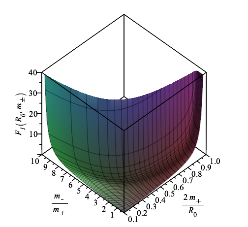
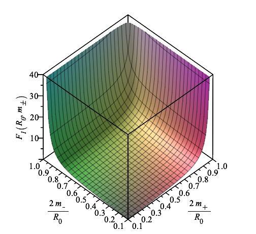
Figure 1: Stability analysis for thin-shell Schwarzschild traversable wormholes, taking into account that $a_{\pm}=0$ and $m_{-}\neq m_{+}$. The surfaces are given by the dimensionless quantity $F_{1}(R_{0},m_{\pm})$, defined by the right-hand-side of inequality (54). The stability regions lie above the surfaces depicted in the plots. We have considered the range $0<x=2m_{+}/R_{0}<1$ and $0<y_{1}=m_{-}/m_{+}<1/x$, in the left plot and $0<y_{2}=2m_{-}/R_{0}<1$ in the right plot, respectively. Note that large stability regions exist for low values of $x=2m_{+}/R_{0}$ and of $y_{1,2}$. For regions close to the event horizon, $x\rightarrow 1$, the stability region decreases in size and only increases significantly for low values of $y_{1}$. See the text for details.

III.2 Vanishing mass: $a_{+}\neq a_{-}$ and $m_{\pm}=0$

Consider now the case of vanishing mass terms $m_{\pm}=0$, with an asymmetry of the bounce parameters $a_{+}\neq a_{-}$.

For this case, inequality (50) reduces to

$$R_{0}^{2}\left[\frac{m_{s}(R_{0})}{R_{0}}\right]^{\prime\prime}\geq F_{2}(R_{0},a_{\pm})=2\left[\frac{\frac{a_{+}^{2}}{R_{0}^{2}}\left(\frac{3}{2}-\frac{a_{+}^{2}}{R_{0}^{2}}\right)}{\left(1-\frac{a_{+}^{2}}{R_{0}^{2}}\right)^{3/2}}+\frac{\frac{a_{-}^{2}}{R_{0}^{2}}\left(\frac{3}{2}-\frac{a_{-}^{2}}{R_{0}^{2}}\right)}{\left(1-\frac{a_{-}^{2}}{R_{0}^{2}}\right)^{3/2}}\right]\,,$$ (55)

and inequality (53) takes the following form

$$R_{0}^{2}\left[4\pi R_{0}^{2}\,\Xi(R_{0})\right]^{\prime\prime}\geq G_{2}(R_{0},a_{\pm})=-\frac{\frac{a_{+}^{2}}{R_{0}^{2}}\left(6-4\frac{a_{+}^{2}}{R_{0}^{2}}+2\frac{a_{+}^{4}}{R_{0}^{4}}\right)}{\left(1-\frac{a_{+}^{2}}{R_{0}^{2}}\right)^{5/2}}-\frac{\frac{a_{-}^{2}}{R_{0}^{2}}\left(6-4\frac{a_{-}^{2}}{R_{0}^{2}}+2\frac{a_{-}^{4}}{R_{0}^{4}}\right)}{\left(1-\frac{a_{-}^{2}}{R_{0}^{2}}\right)^{5/2}}\,.$$ (56)

We now consider the definition of the parameters $x=a_{+}/R_{0}$ and $y=a_{-}/R_{0}$ for convenience, so as to bring infinite $R_{0}$ within a finite region of the plot. That is, $R_{0}\rightarrow\infty$ is represented as $x\rightarrow 0$; and $R_{0}=a_{+},a_{-}$ is equivalent to $x,y=1$. Thus, the parameters $x$ and $y$ are restricted to the ranges $0<x<1$ and $0<y<1$. Inequality (55) is depicted as the upper surface in figure 2 and inequality (56) depicted as the lower surface, and the stability regions are given above the respective surfaces. Thus, the final stability region lies above the upper surface.

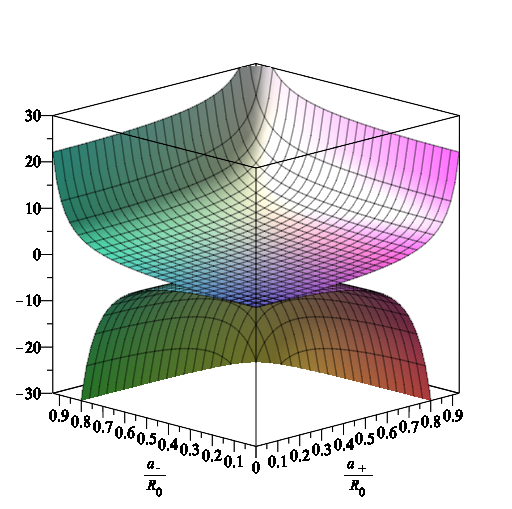
Figure 2: The upper surface depicts the quantity $F_{2}(R_{0},a_{\pm})=R_{0}^{2}\left[m_{s}(R_{0})/R_{0}\right]^{\prime\prime}$, and the stable region lies above the surface of that curve. On the other hand, the function $G_{2}(R_{0},a_{\pm})=R_{0}^{2}\left[4\pi R_{0}^{2}\,\Xi_{0}\right]^{\prime\prime}$ is depicted by the lower surface, and the stable region also lies above the surface of that curve. Thus the final stability region of the solution lies above the upper surface. See the text for more details.

III.3 Asymmetric vanishing parameters: $a_{+}=0$ and $m_{-}=0$

Consider now the case of vanishing interior mass $m_{-}=0$, and vanishing exterior parameter $a_{+}=0$. For this case, the inequality (50) reduces to

$$R_{0}^{2}\left[\frac{m_{s}(R_{0})}{R_{0}}\right]^{\prime\prime}\geq F_{3}(R_{0},m_{+},a_{-})=\left[\frac{\frac{2m_{+}}{R_{0}}\left(1-\frac{3m_{+}}{2R_{0}}\right)}{\left(1-\frac{2m_{+}}{R_{0}}\right)^{3/2}}+\frac{\frac{3a_{-}^{2}}{R_{0}^{2}}\left(1-\frac{2a_{-}^{2}}{3R_{0}^{2}}\right)}{\left(1-\frac{a_{-}^{2}}{R_{0}^{2}}\right)^{3/2}}\right]\,,$$ (57)

and inequality (53) is given by

$$R_{0}^{2}\left[4\pi R_{0}^{2}\,\Xi(R_{0})\right]^{\prime\prime}\geq G_{3}(R_{0},a_{-})=-\frac{2\frac{a_{-}^{2}}{R_{0}^{2}}\left(3-2\frac{a_{-}^{2}}{R_{0}^{2}}+\frac{a_{-}^{4}}{R_{0}^{4}}\right)}{\left(1-\frac{a_{-}^{2}}{R_{0}^{2}}\right)^{5/2}}\,.$$ (58)

These are depicted as the upper and lower surfaces, respectively, in figure 3. As in the previous example, the final stability region of the solution lies above the upper surface.

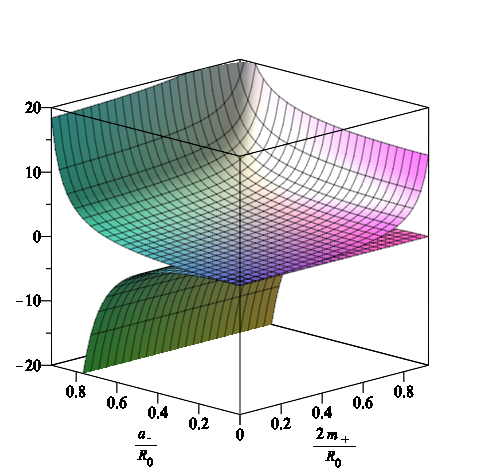
Figure 3: The upper surface depicts the quantity $F_{3}(R_{0},m_{+},a_{-})=R_{0}^{2}\left[m_{s}(R_{0})/R_{0}\right]^{\prime\prime}$, and the stable region lies above that surface. On the other hand, the function $G_{3}(R_{0},a_{-})=R_{0}^{2}\left[4\pi R_{0}^{2}\,\Xi_{0}\right]^{\prime\prime}$ is depicted by the lower surface, and the stable region is also lies above that surface of that plot. Thus, the final stability region of the solution lies above the upper surface. See the text for more details.

III.4 Mirror symmetry: $a_{\pm}=a$ and $m_{\pm}=m$

Consider, for simplicity, the symmetric case, i.e., $a_{\pm}=a$ and $m_{\pm}=m$, so that the stability conditions reduce to:

$$R_{0}^{2}\left[\frac{m_{s}(R_{0})}{R_{0}}\right]^{\prime\prime}\geq 2\left\{{\left[\frac{m}{R_{0}}\left(1-\frac{a^{2}}{R_{0}^{2}}\right)+\frac{a^{2}}{R_{0}^{2}}\left(1-\frac{2m}{R_{0}}\right)\right]^{2}\over\left[\left(1-\frac{2m}{R_{0}}\right)\left(1-\frac{a^{2}}{R_{0}^{2}}\right)\right]^{3/2}}+{\frac{2m}{R_{0}}\left(1-\frac{a^{2}}{R_{0}^{2}}\right)+\frac{3a^{2}}{R_{0}^{2}}\left(1-\frac{2m}{R_{0}}\right)-\frac{4ma^{2}}{R_{0}^{3}}\over\sqrt{\left(1-\frac{2m}{R_{0}}\right)\left(1-\frac{a^{2}}{R_{0}^{2}}\right)}}\right\},$$ (59)

and

$$R_{0}^{2}\left[4\pi R_{0}^{2}\,\Xi_{0}\right]^{\prime\prime} \geq \frac{2a^{2}}{\left(R_{0}^{2}-a^{2}\right)}\left\{-\frac{3R_{0}^{2}(2R_{0}^{2}+a^{2})}{\left(R_{0}^{2}-a^{2}\right)^{2}}\sqrt{\left(1-\frac{2m}{R_{0}}\right)\left(1-\frac{a^{2}}{R_{0}^{2}}\right)}+\frac{4R_{0}^{2}}{\left(R_{0}^{2}-a^{2}\right)}{\frac{m}{R_{0}}\left(1-\frac{a^{2}}{R_{0}^{2}}\right)+\frac{a^{2}}{R_{0}^{2}}\left(1-\frac{2m}{R_{0}}\right)\over\sqrt{\left(1-\frac{2m}{R_{0}}\right)\left(1-\frac{a^{2}}{R_{0}^{2}}\right)}}\right.$$ (60)

$$\qquad\qquad\qquad\left.+{\left[\frac{m}{R_{0}}\left(1-\frac{a^{2}}{R_{0}^{2}}\right)+\frac{a^{2}}{R_{0}^{2}}\left(1-\frac{2m}{R_{0}}\right)\right]^{2}\over\left[\left(1-\frac{2m}{R_{0}}\right)\left(1-\frac{a^{2}}{R_{0}^{2}}\right)\right]^{3/2}}+{\frac{2m}{R_{0}}\left(1-\frac{a^{2}}{R_{0}^{2}}\right)+\frac{3a^{2}}{R_{0}^{2}}\left(1-\frac{2m}{R_{0}}\right)-\frac{4ma^{2}}{R_{0}^{3}}\over\sqrt{\left(1-\frac{2m}{R_{0}}\right)\left(1-\frac{a^{2}}{R_{0}^{2}}\right)}}\right\}\,,$$

respectively.

It is useful to express inequality (59) in the following dimensionless form $F_{4}(R_{0},m,a)=R_{0}^{2}\left[m_{s}(R_{0})/R_{0}\right]^{\prime\prime}$, and inequality (60) as $G_{4}(R_{0},m,a)=R_{0}^{2}\left[4\pi R_{0}^{2}\,\Xi_{0}\right]^{\prime\prime}$. Both surfaces are depicted in figure 4, and the final stability region is situated above the intersection of the surfaces.

Note that we have considered the definition $x=2m/R_{0}$ for convenience, so as to bring infinite $R_{0}$ within a finite region of the plot. That is, $R_{0}\rightarrow\infty$ is represented as $x\rightarrow 0$; and $R_{0}=2m$ is equivalent to $x=1$. Thus, the parameter $x$ is restricted to the range $0<x<1$. We also define the parameter $y=a/R_{0}$, which also lies in the range $0<y<1$. It is interesting to note that the inequality (60) serves to decrease the stability region for high values of $x$ and $y$, as is transparent from figure 4.

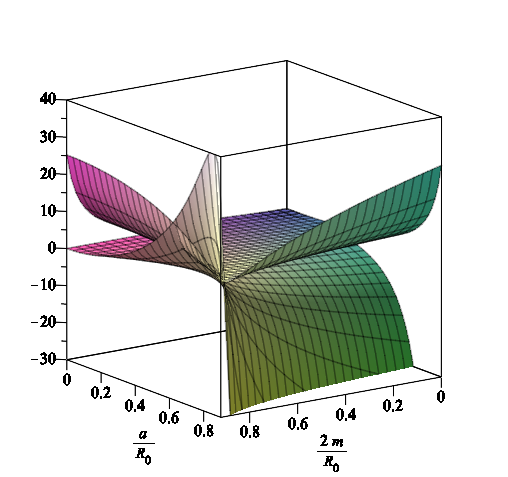
Figure 4: The upper surface depicts the quantity $F_{4}(R_{0},m,a)=R_{0}^{2}\left[m_{s}(R_{0})/R_{0}\right]^{\prime\prime}$, and the stable region lies above that surface. On the other hand, the function $G_{4}(R_{0},m,a)=R_{0}^{2}\left[4\pi R_{0}^{2}\,\Xi_{0}\right]^{\prime\prime}$ is depicted by the lower surface, and the stable region also lies above that surface. The final stability region of the solution lies above the intersection of both surfaces. Note that inequality (60) serves to decrease the stability region for high values of $x$ and $y$. See the text for more details.

III.5 Two specific asymmetric cases

III.5.1 $a_{+}\neq a_{-}$ and $m_{+}=m_{-}$

Consider the case of symmetric masses $m_{\pm}=m$, but with asymmetric bounce parameters $a_{+}\neq a_{-}$. In order to analyse the stability regions we define $a_{+}=\alpha\,a_{-}$, where $\alpha\in\Re^{+}$. Rather than write down the explicit form of the inequalities which are rather lengthy and messy, we present the dimensionless form of inequalities (50) and (53) as the upper and lower surfaces in the plots of figures 5 and 6. Note that the specific case of $\alpha=1$ reduces to the analysis of the mirror symmetry considered in the previous subsection III.4. We consider the dimensionless parameters $x=2m/R_{0}$, and $y=a_{-}/R_{0}$, in order to analyse the stability regions. In the following we separate the cases $\alpha<1$ and $\alpha>1$.

• Specific case of $\alpha<1$: the upper surface and lower surfaces in figure 5 depict the functions $F_{5}(R_{0},m,a_{\pm})=R_{0}^{2}\left[m_{s}(R_{0})/R_{0}\right]^{\prime\prime}$ and $G_{5}(R_{0},m,a_{\pm})=R_{0}^{2}\left[4\pi R_{0}^{2}\,\Xi_{0}\right]^{\prime\prime}$, respectively, and the stability regions representing the inequalities (50) and (53) are the regions above these surfaces. The range of the dimensionless parameters is $0<x,y<1$. We have considered $\alpha=0.9$ in the left plot and $\alpha=0.4$ in the right plot of figure 5. As the final stability region of the solution lies above the intersection of both surfaces, we note that decreasing the value of $\alpha$ qualitatively serves to decrease the lower surface representing inequality (53), and thus increase the final stability region. This is transparent for high values of $x$ and $y$.

• Specific case of $\alpha>1$: the analysis is analogous to the above case and is depicted in figure 6, however, here the left plot is given by $\alpha=1.5$ and the right plot by $\alpha=3$. The range of the dimensionless parameters is given by $0<x<1$ and $0<y<1/\alpha$. As in the previous example, the final stability region of the solution lies above the intersection of both surfaces depicted in figure 6. Note that increasing the value of $\alpha$, serves to decrease the lower surface representing inequality (53), and thus increase the final stability region. However, the range for $y$ decreases for increasing values of $\alpha$ (for $\alpha=1.5$, the range is $0<y<2/3$ and for $\alpha=3$, it is $0<y<1/3$). This analysis is transparent for high values of $x$ and $y$ in figure 6.

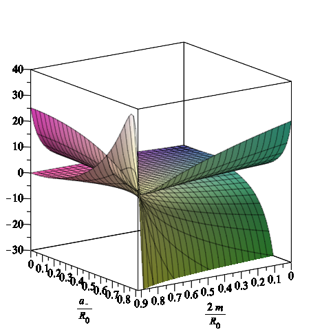
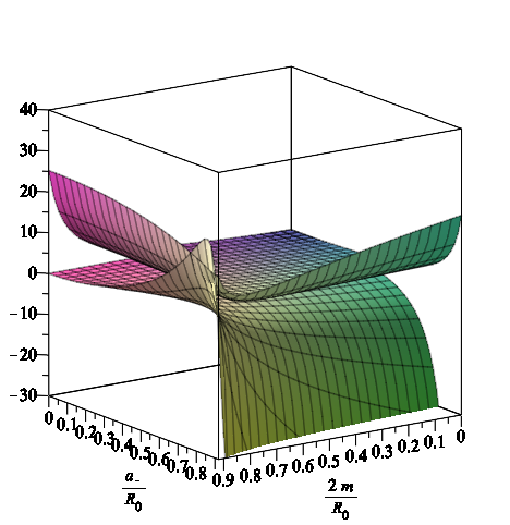
Figure 5: Specific case of $a_{+}=\alpha\,a_{-}$ and $m_{+}=m_{-}$ for $\alpha<1$: The upper surface depicts the quantity $F_{5}(R_{0},m,a_{\pm})=R_{0}^{2}\left[m_{s}(R_{0})/R_{0}\right]^{\prime\prime}$, and the function $G_{5}(R_{0},m,a_{\pm})=R_{0}^{2}\left[4\pi R_{0}^{2}\,\Xi_{0}\right]^{\prime\prime}$ is depicted by the lower surface. The stable regions are given above the surfaces. We have considered $\alpha=0.9$ in the left plot and $\alpha=0.4$ in the right plot. Note that decreasing the value of $\alpha$, serves to decrease the lower surface representing inequality (53), and thus increase the final stability region. See the text for more details.

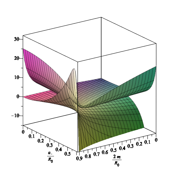
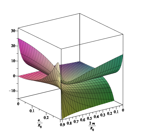
Figure 6: Specific case of $a_{+}=\alpha\,a_{-}$ and $m_{+}=m_{-}$ for $\alpha>1$: The upper surface and lower surfaces depict the quantities $F_{5}(R_{0},m,a_{\pm})=R_{0}^{2}\left[m_{s}(R_{0})/R_{0}\right]^{\prime\prime}$ and $G_{5}(R_{0},m,a_{\pm})=R_{0}^{2}\left[4\pi R_{0}^{2}\,\Xi_{0}\right]^{\prime\prime}$, respectively. The stable regions are given above the surfaces. We have considered $\alpha=1.5$ in the left plot and $\alpha=3$ in the right plot. Note that increasing the value of $\alpha$, serves to decrease the lower surface representing inequality (60), and thus increase the final stability region. However, the range for $y$ decreases for increasing values of $\alpha$ (for $\alpha=1.5$, the range is $0<y<2/3$ and for $\alpha=3$, it is $0<y<1/3$). See the text for more details.

III.5.2 $a_{+}=a_{-}$ and $m_{+}\neq m_{-}$

Here we consider the case of asymmetric masses $m_{\pm}\neq m$, but with symmetric bounce parameters $a_{\pm}=a$, and for simplicity define $m_{+}=\alpha\,m_{-}$, where $\alpha\in\Re^{+}$. As in the specific case previously given above, we present the dimensionless form of inequalities (50) and (53) as the upper and lower surfaces in the plots of figures 7 and 8. We consider the dimensionless parameters $x=2m_{-}/R_{0}$, and $y=a/R_{0}$, in order to analyse the stability regions, and as in the previous example we separate the cases $\alpha<1$ and $\alpha>1$.

• Specific case of $\alpha<1$: the functions $F_{6}(R_{0},m,a_{\pm})=R_{0}^{2}\left[m_{s}(R_{0})/R_{0}\right]^{\prime\prime}$ and $G_{6}(R_{0},m,a_{\pm})=R_{0}^{2}\left[4\pi R_{0}^{2}\,\Xi_{0}\right]^{\prime\prime}$ are depicted by the upper surface and lower surfaces in figure 7, respectively, and the stability regions representing the inequalities (50) and (53) are given above these surfaces. The range of the dimensionless parameters is $0<x,y<1$. We have considered $\alpha=0.9$ in the left plot and $\alpha=0.7$ in the right plot of figure 7. The final stability region of the solution lies above the intersection of both surfaces. Note that decreasing the value of $\alpha$, serves to decrease the lower surface representing inequality (53), and thus increase the final stability region.

• Specific case of $\alpha>1$: analogously to the above case, the stability regions are depicted in figure 8. The left plot is given by $\alpha=1.1$ and the right plot by $\alpha=1.3$. The range of the dimensionless parameters is given by $0<x<1$ and $0<y<1/\alpha$. As in the previous example, the final stability region of the solution lies above the intersection of both surfaces depicted in 8. Note that increasing the value of $\alpha$, serves to decrease the lower surface representing inequality (53), and thus increase the final stability region. However, the range for $y$ decreases for increasing values of $\alpha$.

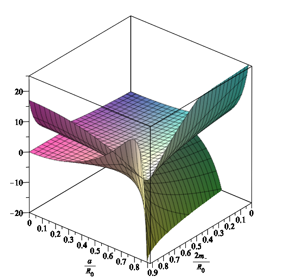
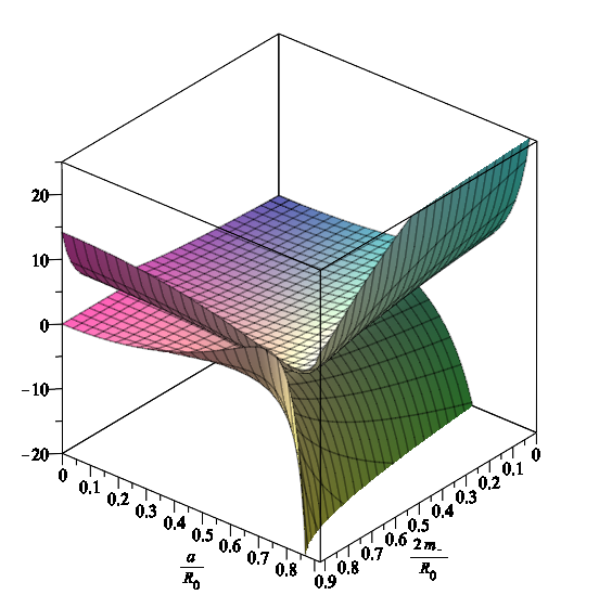
Figure 7: Specific case of $a_{+}=a_{-}$ and $m_{+}=\alpha m_{-}$ for $\alpha<1$. We consider the dimensionless parameters $x=2m_{-}/R_{0}$, and $y=a/R_{0}$. We have considered $\alpha=0.9$ in the left plot and $\alpha=0.7$ in the right plot. Note that decreasing the value of $\alpha$, serves to decrease the lower surface representing inequality (53), and thus increase the final stability region. See the text for more details.

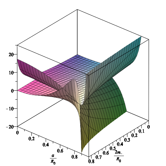
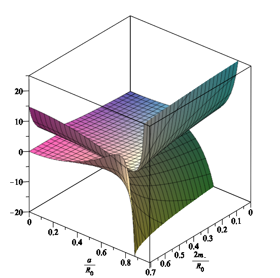
Figure 8: Specific case of $a_{+}=a_{-}$ and $m_{+}=\alpha m_{-}$ for $\alpha>1$. We consider the dimensionless parameters $x=2m{-}/R_{0}$, and $y=a/R_{0}$. We have considered $\alpha=1.1$ in the left plot and $\alpha=1.3$ in the right plot. Note that increasing the value of $\alpha$, serves to decrease the lower surface representing inequality (53), and thus increase the final stability region. See the text for more details.

IV Conclusion

In this article we have considered thin-shell wormholes based on the recently introduced black-bounce spacetimes. Specifically, by matching two black-bounce spherically symmetric spacetimes using the cut-and-paste procedure, we have analyzed the stability and evolution of dynamic thin-shell black-bounce wormholes. We have explored the parameter space of various models depending on the bulk masses $m_{\pm}$, and the values of the bulk bounce parameter $a_{\pm}$, investigating the internal dynamics of the thin-shell connecting the two bulk spacetimes, and demonstrating the existence of suitable stability regions in parameter space. Several of these models are particularly useful in order to emphasize the specific features of these black bounce spacetimes. For instance, some examples are important to assess the simplifications due to symmetry between the two asymptotic regions, while other cases are useful to understand the asymmetry between the two universes used in traversable wormhole construction. Indeed, the interesting physics is encoded in the parameter $a_{\pm}$ which characterizes the scale of the bounce, and that emphasizes the features of these spacetimes. In fact, the presence of the parameter $a_{\pm}$ induces the flux term in the conservation identity, which is responsible for the net discontinuity in the bulk momentum flux which impinges on the shell. Thus, due to this flux term, the bounce parameter places an additional constraint on the stability analysis of the spacetime geometry.

From the linearized stability analysis one may assess and understand the (a)symmetry between the two universes in the traversable wormhole construction. For instance, consider the simple case of vanishing mass $m_{\pm}=0$ and $a_{\pm}\neq 0$ analysed in subsection III.2, where large stability regions exist for $a_{\pm}\ll R_{0}$. However, the low stability region for the specific case of $a_{+}\sim R_{0}$, increases significantly for the asymmetric case of decreasing the value of $a_{-}$. Another interesting example is the asymmetric case analysed in subsection III.3, where we considered $a_{+}=0$ and $m_{-}=0$. Here, the low stability regions for $a_{-}\sim R_{0}$ and $m_{+}\sim R_{0}$ may be significantly increased by decreasing the asymmetric parameters, until large stability regions are present for $a_{-}\ll R_{0}$ and $m_{+}\ll R_{0}$. The mirror symmetric case of $a_{\pm}=a$ and $m_{\pm}=m$, considered in subsection III.4 is of particular interest. Despite the fact that large stability regions exist for $a\ll R_{0}$ and $m\ll R_{0}$, the region at $a\approx R_{0}$ and $m\approx R_{0}$ is of particular interest. Here the flux term constraint kicks in and lowers the stability region significantly. In fact, analysing this specific region for the asymmetric case is particularly interesting, as one may explore the asymmetry between the universes in the wormhole construction by considering the case of $a_{+}\neq a_{-}$ in subsection III.5. More specifically, by varying the relative values of $a_{+}$ and $a_{-}$, the analysis showed that one could increase or decrease the stability regions, and one may assess and understand the (a)symmetry between the two universes in the traversable wormhole construction. In concluding, the constructions considered in this work are sufficiently novel to be interesting, and sufficiently straightforward to be tractable.

References

- (1) L. Flamm, “Beitrage zur Einsteinschen Gravitationstheorie,” Phys. Z. 17, 448 (1916).
- (2) A. Einstein and N. Rosen, “The particle problem in the General Theory of Relativity,” Phys. Rev. 48, 73-77 (1935).
- (3) J. A. Wheeler, “Geons,” Phys. Rev. 97, 511-536 (1955).
- (4) H. G. Ellis, “Ether flow through a drainhole: A particle model in general relativity,” J. Math. Phys. 14, 104 (1973).
- (5) H. G. Ellis, “The evolving, flowless drain hole: a nongravitating particle model in general relativity theory,” Gen. Rel. Grav. 10, 105-123 (1979).
- (6) K. A. Bronnikov, “Scalar-tensor theory and scalar charge,” Acta Phys. Pol. B 4, 251 (1973).
- (7) G. Clement, “Axisymmetric Regular Multiwormhole Solutions in Five-dimensional General Relativity,” Gen. Rel. Grav. 16, 477 (1984).
-
(8)
M. Morris and K.S. Thorne,
“Wormholes in spacetime and their use for interstellar travel: A tool for teaching General Relativity”,
Am. J. Phys. 56, 395 (1988). -
(9)
M. S. Morris, K. S. Thorne and U. Yurtsever,
“Wormholes, Time Machines, and the Weak Energy Condition”,
Phys. Rev. Lett. 61 (1988) 1446. - (10) M. Visser, “Traversable wormholes from surgically modified Schwarzschild space-times”, Nucl. Phys. B 328 (1989) 203 doi:10.1016/0550-3213(89)90100-4 [arXiv:0809.0927 [gr-qc]].
- (11) M. Visser, “Traversable wormholes: Some simple examples”, Phys. Rev. D 39 (1989) 3182 doi:10.1103/PhysRevD.39.3182 [arXiv:0809.0907 [gr-qc]].
- (12) M. Visser, “Wormholes, Baby Universes and Causality”, Phys. Rev. D 41 (1990) 1116. doi:10.1103/PhysRevD.41.1116
- (13) M. Visser, “Quantum Mechanical Stabilization of Minkowski Signature Wormholes”, Phys. Lett. B 242 (1990) 24. doi:10.1016/0370-2693(90)91588-3
- (14) M. Visser, “Wormholes and interstellar travel”, LA-UR-89-1008.
- (15) M. Visser, “Quantum wormholes in Lorentzian signature”, Proceedings of the 1990 DPF Conference, Rice University, Houston, (World Scientific, Singapore, 1990), pp. 0858-0860.
-
(16)
D. Hochberg,
“Lorentzian wormholes in higher order gravity theories”,
Phys. Lett. B 251 (1990) 349.
doi:10.1016/0370-2693(90)90718-L -
(17)
V. P. Frolov and I. D. Novikov,
“Physical Effects in Wormholes and Time Machine”,
Phys. Rev. D 42 (1990) 1057.
doi:10.1103/PhysRevD.42.1057 - (18) M. Visser, “Quantum wormholes”, Phys. Rev. D 43 (1991) 402. doi:10.1103/PhysRevD.43.402
- (19) M. Visser, “Wheeler wormholes and topology change”, Mod. Phys. Lett. A 6 (1991) 2663. doi:10.1142/S0217732391003109
-
(20)
M. Visser,
“From wormhole to time machine: Comments on Hawking’s chronology protection conjecture”,
Phys. Rev. D 47 (1993) 554 doi:10.1103/PhysRevD.47.554 [hep-th/9202090]. - (21) M. Visser, “van Vleck determinants: Traversable wormhole space-time”, Phys. Rev. D 49 (1994) 3963 [gr-qc/9311026].
-
(22)
J. G. Cramer, R. L. Forward, M. S. Morris, M. Visser, G. Benford and G. A. Landis,
“Natural wormholes as gravitational lenses”, Phys. Rev. D 51 (1995) 3117 [astro-ph/9409051]. - (23) S. Kar, “Evolving wormholes and the weak energy condition”, Phys. Rev. D49, 862-865 (1994).
- (24) S. Kar, D. Sahdev, “Evolving Lorentzian wormholes”, Phys. Rev. D53, 722-730 (1996). [gr-qc/9506094].
-
(25)
E. Poisson and M. Visser,
“Thin shell wormholes: Linearization stability”,
Phys. Rev. D 52, 7318 (1995) [arXiv:gr-qc/9506083]. - (26) M. Visser, Lorentzian Wormholes: From Einstein to Hawking (AIP press [now Springer], New York, 1995).
-
(27)
D. Hochberg and M. Visser,
“Geometric structure of the generic static traversable wormhole throat”,
Phys. Rev. D 56 (1997) 4745 [gr-qc/9704082]. -
(28)
M. Visser and D. Hochberg,
“Generic wormhole throats”,
In *Haifa 1997, Internal structure of black holes and spacetime singularities* 249-295 [gr-qc/9710001]. - (29) M. Visser, “Traversable wormholes: The Roman ring”, Phys. Rev. D 55 (1997) 5212 doi:10.1103/PhysRevD.55.5212 [gr-qc/9702043].
- (30) E. Teo, “Rotating traversable wormholes”, Phys. Rev. D58, 024014 (1998). [gr-qc/9803098].
-
(31)
D. Hochberg and M. Visser,
“Null energy condition in dynamic wormholes”,
Phys. Rev. Lett. 81, 746 (1998)
[arXiv:gr-qc/9802048]. - (32) D. Hochberg and M. Visser, “Dynamic wormholes, anti-trapped surfaces, and energy conditions”, Phys. Rev. D 58, 044021 (1998)[arXiv:gr-qc/9802046].
- (33) D. Hochberg and M. Visser, “General dynamic wormholes and violation of the null energy condition”, gr-qc/9901020.
-
(34)
D. Hochberg, C. Molina-París and M. Visser,
“Tolman wormholes violate the strong energy condition”,
Phys. Rev. D 59 (1999) 044011 doi:10.1103/PhysRevD.59.044011 [gr-qc/9810029]. -
(35)
C. Barceló and M. Visser,
“Traversable wormholes from massless conformally coupled scalar fields”,
Phys. Lett. B 466 (1999) 127 [gr-qc/9908029]. -
(36)
M. Visser,
“Gravitational vacuum polarization. 1: Energy conditions in the Hartle–Hawking vacuum”,
Phys. Rev. D 54 (1996) 5103 [gr-qc/9604007]. -
(37)
M. Visser,
“Gravitational vacuum polarization. 2: Energy conditions in the Boulware vacuum”,
Phys. Rev. D 54 (1996) 5116 [gr-qc/9604008]. -
(38)
M. Visser,
“Gravitational vacuum polarization. 3: Energy conditions in the (1+1) Schwarzschild space-time”,
Phys. Rev. D 54 (1996) 5123 [gr-qc/9604009]. -
(39)
M. Visser,
“Gravitational vacuum polarization. 4: Energy conditions in the Unruh vacuum”,
Phys. Rev. D 56 (1997) 936 [gr-qc/9703001]. - (40) M. Visser, “Gravitational vacuum polarization”, gr-qc/9710034.
-
(41)
M. Visser and C. Barceló,
“Energy conditions and their cosmological implications”,
Proceedings of the COSMO99 conference, doi:10.1142/9789812792129_0014 gr-qc/0001099. -
(42)
P. Martín-Moruno and M. Visser,
“Classical and semi-classical energy conditions”,
Fundam. Theor. Phys. 189 (2017) 193
(formerly Lecture Notes in Physics), doi:10.1007/978-3-319-55182-1_9 [arXiv:1702.05915 [gr-qc]]. -
(43)
C. Barceló and M. Visser,
“Brane surgery: Energy conditions, traversable wormholes, and voids”,
Nucl. Phys. B 584 (2000) 415 doi:10.1016/S0550-3213(00)00379-5 [hep-th/0004022]. -
(44)
C. Barceló and M. Visser,
“Scalar fields, energy conditions, and traversable wormholes”,
Class. Quant. Grav. 17 (2000) 3843 [gr-qc/0003025]. -
(45)
N. Dadhich, S. Kar, S. Mukherji and M. Visser,
“ space-times and selfdual Lorentzian wormholes”,
Phys. Rev. D 65 (2002) 064004 doi:10.1103/PhysRevD.65.064004 [gr-qc/0109069]. - (46) C. Barceló and M. Visser, “Twilight for the energy conditions?”, Int. J. Mod. Phys. D 11 (2002) 1553 [gr-qc/0205066].
-
(47)
M. Visser, S. Kar and N. Dadhich,
“Traversable wormholes with arbitrarily small energy condition violations”,
Phys. Rev. Lett. 90, 201102 (2003) [arXiv:gr-qc/0301003]. -
(48)
S. Kar, N. Dadhich and M. Visser,
“Quantifying energy condition violations in traversable wormholes”,
Pramana 63 (2004) 859 [gr-qc/0405103]. - (49) F. S. N. Lobo and M. Visser, “Fundamental limitations on ‘warp drive’ spacetimes”, Class. Quant. Grav. 21, 5871 (2004) [gr-qc/0406083].
-
(50)
A. V. B. Arellano, F. S. N. Lobo,
“Evolving wormhole geometries within nonlinear electrodynamics”,
Class. Quant. Grav. 23, 5811-5824 (2006). [gr-qc/0608003]. - (51) F. S. N. Lobo, “A General class of braneworld wormholes”, Phys. Rev. D75, 064027 (2007). [gr-qc/0701133 [GR-QC]].
-
(52)
F. S. N. Lobo,
“Exotic solutions in General Relativity: Traversable wormholes and ‘warp drive’ spacetimes”,
Classical and Quantum Gravity Research, 1-78, (2008), Nova Science Publishers, ISBN 978-1-60456-366-5,
[arXiv:0710.4474 [gr-qc]]. -
(53)
C. G. Boehmer, T. Harko and F. S. N. Lobo,
“Conformally symmetric traversable wormholes”,
Phys. Rev. D 76, 084014 (2007) doi:10.1103/PhysRevD.76.084014 [arXiv:0708.1537 [gr-qc]]. -
(54)
C. G. Boehmer, T. Harko and F. S. N. Lobo,
“Wormhole geometries with conformal motions”,
Class. Quant. Grav. 25, 075016 (2008) doi:10.1088/0264-9381/25/7/075016 [arXiv:0711.2424 [gr-qc]]. - (55) F. S. N. Lobo, “General class of wormhole geometries in conformal Weyl gravity”, Class. Quant. Grav. 25, 175006 (2008). [arXiv:0801.4401 [gr-qc]].
-
(56)
F. S. N. Lobo, M. A. Oliveira,
“Wormhole geometries in modified theories of gravity”,
Phys. Rev. D80, 104012 (2009). [arXiv:0909.5539 [gr-qc]]. -
(57)
N. Montelongo-García, F. S. N. Lobo,
“Wormhole geometries supported by a nonminimal curvature-matter coupling”,
Phys. Rev. D82, 104018 (2010). [arXiv:1007.3040 [gr-qc]]. -
(58)
N. Montelongo-García, F. S. N. Lobo,
“Nonminimal curvature-matter coupled wormholes with matter satisfying the null energy condition”,
Class. Quant. Grav. 28, 085018 (2011). [arXiv:1012.2443 [gr-qc]]. -
(59)
C. G. Boehmer, T. Harko and F. S. N. Lobo,
“Wormhole geometries in modified teleparralel gravity and the energy conditions”,
Phys. Rev. D 85 (2012) 044033 [arXiv:1110.5756 [gr-qc]]. -
(60)
N. Montelongo-García, F. S. N. Lobo and M. Visser,
“Generic spherically symmetric dynamic thin-shell traversable wormholes in standard general relativity”,
Phys. Rev. D 86 (2012) 044026 [arXiv:1112.2057 [gr-qc]]. -
(61)
F. S. N. Lobo, P. Martín-Moruno, N. Montelongo-García and M. Visser,
“Linearised stability analysis of generic thin shells”, arXiv:1211.0605 [gr-qc]. -
(62)
T. Harko, F. S. N. Lobo, M. K. Mak and S. V. Sushkov,
“Modified-gravity wormholes without exotic matter”,
Phys. Rev. D 87 (2013) no.6, 067504 [arXiv:1301.6878 [gr-qc]]. -
(63)
M. R. Mehdizadeh, M. Kord Zangeneh and F. S. N. Lob0,
“Einstein-Gauss-Bonnet traversable wormholes satisfying the weak energy condition”,
Phys. Rev. D 91, no. 8, 084004 (2015) [arXiv:1501.04773 [gr-qc]]. -
(64)
M. Kord Zangeneh, F. S. N. Lobo and M. H. Dehghani,
“Traversable wormholes satisfying the weak energy condition in third-order Lovelock gravity”,
Phys. Rev. D 92, no. 12, 124049 (2015) [arXiv:1510.07089 [gr-qc]]. -
(65)
F. S. N. Lobo, M. Bouhmadi-López, P. Martín-Moruno, N. Montelongo-García and M. Visser,
“A novel approach to thin-shell wormholes and applications”, arXiv:1512.08474 [gr-qc]. -
(66)
P. Boonserm, T. Ngampitipan, A. Simpson and M. Visser,
“Exponential metric represents a traversable wormhole”,
Phys. Rev. D 98 (2018) no.8, 084048 [arXiv:1805.03781 [gr-qc]]. - (67) A. Simpson and M. Visser, “Black-bounce to traversable wormhole”, JCAP 1902 (2019) 042 [arXiv:1812.07114 [gr-qc]].
-
(68)
A. Simpson, P. Martín-Moruno and M. Visser,
“Vaidya spacetimes, black-bounces, and traversable wormholes”,
Class. Quant. Grav. 36 (2019) no.14, 145007 [arXiv:1902.04232 [gr-qc]]. -
(69)
F. S. N. Lobo,
“Wormholes, Warp Drives and Energy Conditions”,
Fundam. Theor. Phys. 189, pp. (2017),
(formerly Lecture Notes in Physics), Springer Nature Switzerland AG. - (70) J. L. Rosa, J. P. S. Lemos and F. S. N. Lobo, “Wormholes in generalized hybrid metric-Palatini gravity obeying the matter null energy condition everywhere,” Phys. Rev. D 98, no. 6, 064054 (2018) [arXiv:1808.08975 [gr-qc]].
- (71) N. Sen, “Über die grenzbedingungen des schwerefeldes an unsteig keitsflächen”, Ann. Phys. (Leipzig) 73, 365 (1924).
-
(72)
K. Lanczos, “Flächenhafte verteiliung der materie in der
Einsteinschen gravitationstheorie”,
Ann. Phys. (Leipzig) 74, 518 (1924). - (73) G. Darmois, “Mémorial des sciences mathématiques XXV”, Fascicule XXV ch V (Gauthier-Villars, Paris, France, 1927).
- (74) S. O’Brien and J. L. Synge, Commun. Dublin Inst. Adv. Stud. A., no. 9 (1952);
- (75) A. Lichnerowicz, “Théories Relativistes de la Gravitation et de l’Electromagnetisme”, Masson, Paris (1955).
-
(76)
W. Israel, “Singular hypersurfaces and thin shells in general
relativity”, Nuovo Cimento 44B, 1 (1966);
and corrections in ibid. 48B, 463 (1966). - (77) E. F. Eiroa and G. E. Romero “Linearized stability of charged thin-shell wormholes”, Gen. Rel. Grav. 36 651-659 (2004) [arXiv:gr-qc/0303093].
- (78) F. S. N. Lobo and P. Crawford, “Linearized stability analysis of thin shell wormholes with a cosmological constant”, Class. Quant. Grav. 21, 391 (2004) [arXiv:gr-qc/0311002].
- (79) J. Fraundiener, C. Hoenselaers and W. Konrad, “A shell around a black hole”, Class. Quant. Grav. 7, 585 (1990).
- (80) P. R. Brady, J. Louko and E. Poisson, “Stability of a shell around a black hole”, Phys. Rev. D 44, 1891 (1991).
- (81) S. M. C. V. Gonçalves, “Relativistic shells: Dynamics, horizons, and shell crossing”, Phys. Rev. D 66, 084021(2002) [arXiv:gr-qc/0212124].
-
(82)
J. P. S. Lemos, F. S. N. Lobo and S. Q. de Oliveira,
“Morris-Thorne wormholes with a cosmological constant”,
Phys. Rev. D 68, 064004 (2003) [arXiv:gr-qc/0302049]. - (83) F. S. N. Lobo, “Energy conditions, traversable wormholes and dust shells”, Gen. Rel. Grav. 37 (2005) 2023 [arXiv:gr-qc/0410087].
- (84) F. S. N. Lobo, “Surface stresses on a thin shell surrounding a traversable wormhole”, Class. Quant. Grav. 21 4811 (2004) [arXiv:gr-qc/0409018].
-
(85)
J. P. S. Lemos and F. S. N. Lobo, “Plane symmetric traversable
wormholes in an anti-de Sitter background”,
Phys. Rev. D 69, 104007 (2004) [arXiv:gr-qc/0402099]. - (86) S. Sushkov, “Wormholes supported by a phantom energy”, Phys. Rev. D 71, 043520 (2005) [arXiv:gr-qc/0502084].
- (87) F. S. N. Lobo, “Phantom energy traversable wormholes”, Phys. Rev. D 71, 084011 (2005) [arXiv:gr-qc/0502099].
- (88) F. S. N. Lobo, P. Crawford, “Stability analysis of dynamic thin shells”, Class. Quant. Grav. 22, 4869-4886 (2005). [gr-qc/0507063];
- (89) F. S. N. Lobo, “Stability of phantom wormholes”, Phys. Rev. D71, 124022 (2005) [gr-qc/0506001].
- (90) E. F. Eiroa and C. Simeone, “Cylindrical thin shell wormholes”, Phys. Rev. D 70, 044008 (2004) [arXiv:gr-qc/0404050];
-
(91)
E. F. Eiroa and C. Simeone,
“Thin-shell wormholes in dilaton gravity”,
Phys. Rev. D 71, 127501 (2005).
[arXiv:gr-qc/0502073]; -
(92)
M. Thibeault, C. Simeone and E. F. Eiroa,
“Thin-shell wormholes in Einstein-Maxwell theory with a Gauss-Bonnet term”,
Gen. Rel. Grav. 38, 1593 (2006) [arXiv:gr-qc/0512029]. - (93) F. Rahaman, M. Kalam and S. Chakraborty, “Thin shell wormholes in higher dimensional Einstein-Maxwell theory”, Gen. Rel. Grav. 38, 1687 (2006) [arXiv:gr-qc/0607061].
-
(94)
F. Rahaman, M. Kalam and S. Chakraborti,
“Thin shell wormhole in heterotic string theory”,
Int. J. Mod. Phys. D 16, 1669 (2007) [arXiv:gr-qc/0611134]. -
(95)
C. Bejarano, E. F. Eiroa and C. Simeone,
“Thin-shell wormholes associated with global cosmic strings”,
Phys. Rev. D 75, 027501 (2007) [arXiv:gr-qc/0610123]. -
(96)
E. F. Eiroa and C. Simeone,
“Stability of Chaplygin gas thin-shell wormholes”,
Phys. Rev. D 76, 024021 (2007)
[arXiv:0704.1136 [gr-qc]]. -
(97)
J. P. S. Lemos and F. S. N. Lobo,
“Plane symmetric thin-shell wormholes: Solutions and stability”,
Phys. Rev. D 78, 044030 (2008) [arXiv:0806.4459 [gr-qc]]. -
(98)
E. F. Eiroa, M. G. Richarte and C. Simeone,
“Thin-shell wormholes in Brans–Dicke gravity”,
Phys. Lett. A 373, 1 (2008) [Erratum-ibid. 373, 2399 (2009)] [arXiv:0809.1623 [gr-qc]]. -
(99)
E. F. Eiroa,
“Thin-shell wormholes with a generalized Chaplygin gas”,
Phys. Rev. D 80, 044033 (2009)
[arXiv:0907.2205 [gr-qc]]. -
(100)
E. F. Eiroa,
“Stability of thin-shell wormholes with spherical symmetry”,
Phys. Rev. D 78, 024018 (2008)
[arXiv:0805.1403 [gr-qc]]. -
(101)
E. F. Eiroa and C. Simeone,
“Some general aspects of thin-shell wormholes with cylindrical symmetry”,
Phys. Rev. D 81, 084022 (2010) [arXiv:0912.5496 [gr-qc]]. -
(102)
S. H. Mazharimousavi, M. Halilsoy and Z. Amirabi,
“Stability of thin-shell wormholes supported by ordinary matter in Einstein-Maxwell-Gauss-Bonnet gravity”,
Phys. Rev. D 81, 104002 (2010) [arXiv:1001.4384 [gr-qc]]. -
(103)
G. A. S. Dias and J. P. S. Lemos,
“Thin-shell wormholes in -dimensional general relativity: Solutions, properties, and stability”,
Phys. Rev. D 82, 084023 (2010) [arXiv:1008.3376 [gr-qc]]. -
(104)
X. Yue and S. Gao,
“Stability of Brans-Dicke thin shell wormholes”,
Phys. Lett. A 375, 2193 (2011)
[arXiv:1105.4310 [gr-qc]]. -
(105)
A. DeBenedictis, R. Garattini and F. S. N. Lobo,
“Phantom stars and topology change”, Phys. Rev. D 78, 104003 (2008)
[arXiv:0808.0839 [gr-qc]]. -
(106)
P. Musgrave and K. Lake,
“Junctions and thin shells in general relativity using computer algebra I: The Darmois-Israel formalism”,
Class. Quant. Grav. 13 1885 (1996) [arXiv:gr-qc/9510052]. -
(107)
M. Ishak and K. Lake, “Stability of transparent spherically
symmetric thin shells and wormholes”,
Phys. Rev. D 65 044011 (2002) [arXiv:gr-qc/0108058]. - (108) S. W. Hawking and G.F.R. Ellis, The Large Scale Structure of Spacetime, (Cambridge University Press, Cambridge 1973).
- (109) K. A. Bronnikov, V. N. Melnikov and H. Dehnen, “Regular black holes and black universes,” Gen. Rel. Grav. 39, 973 (2007) [gr-qc/0611022].
- (110) K. A. Bronnikov, V. N. Melnikov and H. Dehnen, “On a general class of brane world black holes,” Phys. Rev. D 68, 024025 (2003) [gr-qc/0304068].
- (111) P. O. Mazur and E. Mottola, “Gravitational condensate stars: An alternative to black holes”, gr-qc/0109035.
- (112) P. O. Mazur and E. Mottola, “Dark energy and condensate stars: A quantum alternative to classical black holes”,
- (113) P. O. Mazur and E. Mottola, “Dark energy and condensate stars: Casimir energy in the large”, gr-qc/0405111.
-
(114)
P. O. Mazur and E. Mottola,
“Gravitational vacuum condensate stars”,
Proc. Nat. Acad. Sci. 101 (2004) 9545
doi:10.1073/pnas.0402717101 [gr-qc/0407075]. -
(115)
M. Visser, D. L. Wiltshire,
“Stable gravastars: An Alternative to black holes?”,
Class. Quant. Grav. 21 (2004) 1135-1152
[gr-qc/0310107]. -
(116)
C. Cattöen, T. Faber and M. Visser,
“Gravastars must have anisotropic pressures”,
Class. Quant. Grav. 22, 4189 (2005)
[gr-qc/0505137]. - (117) F. S. N. Lobo, “Stable dark energy stars”, Class. Quant. Grav. 23, 1525-1541 (2006). [gr-qc/0508115].
-
(118)
F. S. N. Lobo and A. V. B. Arellano,
“Gravastars supported by nonlinear electrodynamics”,
Class. Quant. Grav. 24, 1069 (2007) [gr-qc/0611083]. -
(119)
P. Martín-Moruno, N. Montelongo-García, F. S. N. Lobo and M. Visser,
“Generic thin-shell gravastars”,
JCAP 1203 (2012) 034 [arXiv:1112.5253 [gr-qc]]. -
(120)
F. S. N. Lobo, P. Martín-Moruno, N. Montelongo-García and M. Visser,
“Novel stability approach of thin-shell gravastars”,
arXiv:1512.07659 [gr-qc].