Double parton correlations in mesons within AdS/QCD soft-wall models: a first comparison with lattice data

Abstract

Double parton distribution functions (dPDFs), entering the double parton scattering (DPS) cross section, are unknown fundamental quantities encoding new interesting properties of hadrons. Here, the pion dPDFs are investigated within different holographic QCD quark models in order to access their basic features. Results of the calculation,s obtained within the AdS/QCD soft-wall approach, have been compared with predictions of lattice QCD evaluations of the pion two-current correlation functions. The present analysis confirms that double parton correlations, affecting dPDFs, are very important and not direct accessible from generalised parton distribution functions and electromagnetic form factors. The comparison between lattice data and quark model calculations unveils the relevance of the contributions of high partonic Fock states in the pion. Nevertheless, by using a complete general procedure, results of lattice QCD have been used, for the first time, to estimate the mean value of the so called $\sigma_{eff}$, a relevant experimental observable for DPS processes. In addition, the results of the first calculations of the $\rho$ meson dPDFs are discussed in order to make predictions.

1 Introduction

In the last few years, great attention has been devoted to theoretical and experimental studies of multiple parton interactions (MPI), due to the large demand of detailed description of hadronic final states required at the LHC [1, 2]. The inclusion of MPI in experimental analyses is fundamental for the research of New Physics, being MPI a source of background. The simplest case of MPI is the double parton scattering (DPS) [3, 4], where two partons of an hadron simultaneously interact with other two partons of the other colliding hadron. As discussed in a recent review [5], the measurements of DPS processes are mandatory to access unknown double parton correlations (DPCs) in the proton. Moreover, the DPS cross section depends on a new quantity called double parton distribution functions (dPFDs) which encode the probability of finding two partons, with given flavors, longitudinal momentum fractions ($x_{1},x_{2}$) and relative transverse distance $d_{\perp}$ [1, 6, 7]. If measured, dPDFs would therefore represent a novel tool to access the three-dimensional hadron structure [8, 9]. In fact, dPDFs provide new fundamental information, complementary to those obtained by using generalised parton distribution functions (GPDs) [10]. However, for the moment being, no data for the proton dPDFs have been so far collected. Furthermore, dPDFs are non perturbative objects in QCD not directly accessible from the theory. It is therefore useful to estimate them at low momentum scales ($\sim\Lambda_{QCD}$), for example by using quark models  [11, 12, 13, 14]. In addition to several general analyses on dPDFs  [6, 8, 15, 16, 17, 18], a lattice QCD investigation on two-current correlations in the pion has been published very recently  [19]. In the present analysis, we take advantage of the lattice data, to test quark model predictions for the pion dPDFs. The calculations of the latter have been shown for the first time in Ref. [20] and then within the Nambu-Jona-Lasinio (NJL) model  [21, 22, 23]. In particular, by following the line of Ref. [20], we consider here AdS/QCD soft-wall quark models. Let us mention that the mean value of $\sigma_{eff}$, sensitive to dPDFs, has been already calculated within an holographic QCD model for the proton target  [24]. The models here used are inspired by the so called AdS/CFT correspondence [25, 26], which relates a supersymmetric conformal field theory with a classical graviational one in an anti-de-Sitter space. In the so called bottom-up approach, one implements fundamental properties of QCD by generating a theory in which conformal symmetry is asymptotically restored  [27, 28, 29, 30, 31]. Let us mention that this approach has been successfully applied to access non perturbative features of QCD, for example the description of the spectrum of glueballs, hadrons, form factors (ffs) and different kind of parton distribution functions (PDFs)  [32, 33, 34, 35, 36, 37, 38, 39, 40, 41, 42, 43]. In the present investigation we discuss the calculations of the pion dPDFs and their first moments within the AdS/QCD approach. Comparisons with lattice outcomes will test the predictive power of these models and provide new fundamental constraints for their future improvements. In the last part of the present investigation, predictions for the $\rho$ dPDFs will be shown for the first time. The paper is organised as follows.

In Sect. 2 the formalism to describe dPDFs and related quantities within the Light-Front (LF) approach is shown. In Sect. 3 a brief recapitulation of the main lattice evaluation of moments of dPDFs [19] will be presented. In Sect. 4 details on the adopted AdS/QCD models will be discussed. In Sect. 5 numerical calculations of dPDFs and related quantities will be shown, also including the comparisons with lattice data. In Sect. 6 the first study of the $\rho$ dPDFs is presented.

2 Meson Double PDF within the Light-Front approach

In this formal section, the main strategy to obtain a suitable expression of the mesonic dPDFs, for quark model calculations, will be presented. In particular, the essential steps of this procedure have been previously developed in Refs. [20, 44] and they are here summarised. In particular we consider the Light-Front (LF) approach [45, 46] together with the LF wave function representation of the hadronic state [47, 48]. In this scenario, the meson (M) state $|M,P\rangle$, with momentum $P^{\mu}$, can be decomposed in a coherent sum over partonic Fock states. The relative contribution of a given Fock state to the meson is encoded in the so called LF wave function (w.f.) $\psi$. The latter contains all non-perturbative information on the meson structure. Of course, the LF w.f. cannot be evaluated from first principles, i.e. the QCD. In this scenario, constituent quark models represent suitable tools to evaluate the w.f. and then to explore basic non perturbative features of different kind of distributions, such as parton distribution functions, form factors and dPDFs. Indeed, all these quantities can be described in terms of the LF wave function. In the present analysis we focus our attention on dPDFs. As already mentioned, these quantities encodes novel information on the hadron structure which cannot be obtained through one-body functions such as generalised parton distributions and transverse momentum dependent PDFs (TMDs). Since the main purpose of this investigation is the comparison between quark model calculations with those obtained within the lattice framework [19], here we consider the unpolarized dPDFs which depend on the Dirac matrix $\gamma^{\mu}$. The double PDFs can be formally defined through a light-cone correlator [6]:

$$F_{q_{1}q_{2}}(x_{1},x_{2},{\bf k_{\perp}})={P^{+}\over 4}\int d^{2}{\bf y_{\perp}}e^{-i{\bf y_{\perp}}\cdot{\bf k_{\perp}}}\int dy^{-}\int dz^{-}_{1}dz_{2}^{-}$$ (1)

$$\times{e^{-ix_{1}P^{+}z^{-}_{1}-ix_{2}P^{+}z^{-}_{2}}\over(2\pi)^{2}}\langle M,{\bf 0}|\mathcal{O}_{q_{1}}(0,z_{1})\mathcal{O}_{q_{2}}(y,z_{2})|M,{\bf{\bf 0}}\rangle\Big{|}_{y^{+}=z^{+}_{1}=z_{2}^{+}=0}^{{\bf z_{1\perp}=z_{2\perp}}=0}~{},$$

where, for generic 4-vectors $y$ and $z$, the operator $\mathcal{O}_{q}(y,z)$ for the quark of flavor $q$ reads:

$$\mathcal{O}_{q}(y,z)=\bar{q}\left(y-{1\over 2}z\right)\gamma^{+}q\left(y+{1\over 2}z\right)~{},$$ (2)

and $q(z)$ is the LF quark field operator. In order to find a suitable expression of the dPDF, we consider the Fock decomposition of the mesonic state [47, 48] and keep only the $|q\bar{q}\rangle$ contribution [20]. In fact, for the moment being, an explicit expression for the LF wave function of, e.g., the $|q\bar{q}q\bar{q}\rangle$ state, is not available. Therefore, the meson state reads:

$$|M,{\bf P_{\perp}}\rangle =\sum_{h,\bar{h}}\int\dfrac{dx_{1}~{}dx_{2}}{\sqrt{x_{1}x_{2}}}\dfrac{d^{2}{\bf k_{1\perp}}d^{2}\bf k_{2\perp}}{2(2\pi)^{3}}\delta^{(2)}({\bf k_{1\perp}+k_{2\perp}})|x_{1},{\bf k_{1\perp}}+x_{1}{\bf P_{\perp}},h\rangle|x_{2},{\bf k_{2\perp}}+x_{2}{\bf P_{\perp}},\bar{h}\rangle$$

$$\times~{}\delta(1-x_{1}-x_{2})\psi^{M}_{h,\bar{h}}(x_{1},x_{2},{\bf k_{1\perp},k_{2\perp}})~{}.$$ (3)

Here, $h$ and $\bar{h}$ represent the parton helicities, $x_{i}=k_{i}^{+}/P^{+}$ and ${\bf k_{i\perp}}$ the quark longitudinal momentum fraction and its transverse momentum, respectively, and $P^{\mu}$ is the meson 4-momentum. The light cone components of a generic 4-vector are defined by $l^{\pm}=l^{0}\pm l^{3}$. In Eq. (2), $\psi^{M}_{h,\bar{h}}(x_{1},x_{2},{\bf k_{1\perp},k_{2\perp}})$ is the LF meson wave-function, whose normalisation is chosen to be

$${1\over 2}\sum_{h,\bar{h}}\int dx_{1}dx_{2}{d^{2}{\bf k_{1\perp}}d^{2}{\bf k_{2\perp}}\over 16\pi^{3}}\delta(1-x_{1}-x_{2})\delta^{(2)}({\bf k_{1\perp}{\bf+}k_{2\perp}})|\psi^{M}_{h,\bar{h}}(x_{1},x_{2},{\bf k_{1\perp},k_{2\perp}})|^{2}=1~{}.$$ (4)

The w.f. $\psi^{M}_{h,\bar{h}}(x_{1},x_{2},{\bf k_{1\perp},k_{2\perp}})$ determines the structure of the state. The direct expression of the dPDF in terms of the above quantity can be obtained by following the procedure developed in Refs. [14, 20, 44]. In the Appendix A, details on the convention for the quark-antiquark field operator and anticommutation relations, between creation-annihilation operators [32], are shown. Finally, the meson dPDF reads:

$$F_{q_{1}\bar{q}_{2}}(x_{1},x_{2},{\bf k_{\perp}}) ={1\over 2}\sum_{h,\bar{h}}\int{d^{2}{\bf k_{1\perp}}\over 2(2\pi)^{3}}\psi^{M}_{h,\bar{h}}(x_{1},x_{2},{\bf k_{1\perp}},-{\bf k_{1\perp}})\psi_{h,\bar{h}}^{*M}(x_{1},x_{2},{\bf k_{1\perp}+k_{\perp}},-{\bf k_{1\perp}-k_{\perp}})\delta(1-x_{1}-x_{2})$$

$$=f_{2}^{M}(x_{1},{\bf k_{\perp}})\delta(1-x_{1}-x_{2}).$$ (5)

In the above expression, $q_{1}$ and $\bar{q}_{2}$ are the flavors of the constituent quarks. Due to momentum conservation, $x_{2}=1-x_{1}$ and ${\bf k_{2\perp}}=-{\bf k_{1\perp}}$; thus we define $\psi_{h,\bar{h}}(x_{1},{\bf k_{1\perp}})=\psi^{\pi}_{h,\bar{h}}(x_{1},1-x_{1},{\bf k_{1\perp}},{\bf-k_{1\perp}})$ for brevity.

Since as already mentioned, the comparison with lattice data is fundamental in the present investigation, we are mainly interested in moments of dPDFs, i.e. the integrals over $x_{1}$ and $x_{2}$ of Eq. (5). Thus $f_{2}^{M}(x_{1},{\bf k_{\perp}})$ in Eq. (5), is the quantity that will be calculated within constituent quark models:

$$f_{2}^{M}(x,{\bf k_{\perp}}) =\int_{0}^{1}dx_{2}~{}F_{q_{1}\bar{q}_{2}}(x,x_{2},{\bf k_{\perp}})={1\over 2}\sum_{h,\bar{h}}\int{d^{2}{\bf k_{1\perp}}\over 2(2\pi)^{3}}\psi^{M}_{h,\bar{h}}(x,{\bf k_{1\perp}})\psi_{h,\bar{h}}^{*M}(x,{\bf k_{1\perp}+k_{\perp}}).$$ (6)

As shown in Refs. [14, 15, 16], dPDFs evaluated at ${\bf k_{\perp}}=0$ are related to the PDF. Here and in the following, the meson PDFs are specified by the subscript “1” , i.e. $f_{1}^{M}(x)$. As one might notice, if only a two-body Fock state is considered in Eq. (2), the dPDF would be essentially an unintegrated PDF. In the proton case, where the $|qqq\rangle$ state is the dominant one, the above feature is not valid. In this analysis we make use of different quark models to identify general non perturbative features of dPDFs. Therefore, the following ratio is studied [13, 14] to emphasise the role of correlations between the $x$ and ${\bf k_{\perp}}$ dependence:

$$r_{k}(x,k_{\perp})={f_{2}^{M}(x,k_{\perp})\over f_{2}^{M}(0.4,k_{\perp})}~{};$$ (7)

in fact, if a factorised ansatz for dPDFs were valid, for example $f_{2}^{M}(x,k_{\perp})\sim f_{2,x}(x)f_{2,k_{\perp}}(k_{\perp})$, then the ratio $r_{k}(x,k_{\perp})$ would not depend on $k_{\perp}$. For details on the calculations of this quantity, in the proton case, see Refs. [13, 14, 8, 49]. Let us remind that this kind of ansatz is often used in experimental analyses.

In closing this section, we note that the dPDFs depend on two momentum scales. Therefore, in order to make useful predictions, the perturbative QCD evolution of dPDFs should be properly included in the analyses. Moreover, as shown in several papers, see e.g. Refs. [14, 55], the evolution procedure can reduce the impact of $x_{1}-x_{2}$ correlations. However, since the pQCD evolution equations of dPDFs do not involve the $k_{\perp}$ dependence, correlations between $x$ and $k_{\perp}$ can be relevant also at high energy scales. Such a conclusion has been discussed in Ref. [20] for the pion, and in Refs. [8, 49] for the proton. Furthermore, since for the moment being we are mainly interested in the first moment of dPDFs, we take both scales equal to the hadronic one. For evolution effects in the pion dPDFs see Ref. [20].

2.1 Moments of dPDFs

As already mentioned, in the present study we are mainly interested on the first moment of the pion dPDF. Results of the calculations of this quantity will be compared to that obtained within the lattice [19]. The physical interpretation of the first moment of dPDFs is here discussed. As shown in Refs. [8, 50, 9], the latter can be interpreted as a double form factor. This quantity, usually called effective form factor (eff), can be defined as follows:

$$F_{2}(k_{\perp}^{2})=\int_{0}^{1}dx_{1}~{}\int_{0}^{1-x_{1}}dx_{2}~{}F_{q_{1}q_{2}}(x_{1},x_{2},{\bf k_{\perp}})~{}.$$ (8)

For unpolarized dPDFs, the eff does not depend on the direction of ${\bf k_{\perp}}$. The above definition is general and also valid for many-body systems. Moreover, one should notice that the normalisation of the LF wave function relies in the condition: $F_{2}(0)=1$. Physically, the latter ensures that the Fourier Transform (FT) of the eff can be interpreted as the probability of finding two partons with a given transverse distance ${\bf d_{\perp}}$. This quantity is indeed the conjugate variable to ${\bf k_{\perp}}$. Let us stress that a pre-factor in Eq. (8), depending on the kind of hadron, could appear according to the dPDF sum rules [15]. In the meson case, where only a $q\bar{q}$ state is considered, the eff reads:

$$F_{2}(k_{\perp}^{2}) =\int_{0}^{1}dx~{}f_{2}(x,{\bf k_{\perp}})={1\over 2}\sum_{h,\bar{h}}\int_{0}^{1}dx~{}\int{d^{2}{\bf k_{1\perp}}\over 2(2\pi)^{3}}~{}\psi_{h,\bar{h}}(x,{\bf k_{1\perp}})\psi_{h,\bar{h}}^{*}(x,{\bf k_{1\perp}+k_{\perp}})~{}.$$ (9)

The above quantity will be calculated in the next sections and compared with that extracted from the lattice QCD  [19].

2.2 An approximation in terms of one body quantities

In order to phenomenologically estimate the magnitude of the DPS cross section in proton-proton collisions, an approximate relation between GPDs and dPDFs is often assumed in experimental analyses  [51, 52]. In fact, by introducing a complete set of states in the correlator (1) and keeping only the mesonic contribution, one gets

$$F_{q_{1}\bar{q}_{2}}(x_{1},x_{2},{\bf k_{\perp}}) \sim{P^{+}\over 4}\int d^{2}{\bf y_{\perp}}e^{-i{\bf y_{\perp}}\cdot{\bf k_{\perp}}}\int dy^{-}\int dz^{-}_{1}dz_{2}^{-}\int\dfrac{dP^{\prime+}d^{2}{\bf P^{\prime}_{\perp}}}{2(2\pi)^{3}P^{\prime+}}{e^{-ix_{1}P^{+}z^{-}_{1}-ix_{2}P^{+}z^{-}_{2}}\over(2\pi)^{2}}$$

$$\times\langle M,{\bf 0}|\mathcal{O}_{q_{1}}(0,z_{1})|M,{\bf P^{\prime}_{\perp}}\rangle\langle M,{\bf P^{\prime}_{\perp}}|\mathcal{O}_{\bar{q}_{2}}(y,z_{2})|M,{\bf{\bf 0}}\rangle\Big{|}_{y^{+}=z^{+}_{1}=z_{2}^{+}=0}^{{\bf z_{1\perp}=z_{2\perp}}=0}~{}.$$ (10)

By using the strategy already discussed in the previous section, one finally finds:

$$F_{q_{1}\bar{q}_{2}}(x_{1},x_{2},{\bf k_{\perp}}) \sim H_{q_{1}}(x_{1},{\bf k_{\perp}})H_{\bar{q}_{2}}(1-x_{2},-{\bf k_{\perp}})~{},$$ (11)

where $H_{q}(x,{\bf k_{\perp}})=H_{q}(x,\xi=0,{\bf k_{\perp}})$, is the meson GPD at zero skewness (see Refs. [53, 54] for useful reports on GPDs). Let us mention that the above expression has been tested, in the proton case, by using a LF quark model  [55]. The integral over $x_{2}$ of Eqs. (5) and (11) leads to

$$f^{M}_{2}(x,{\bf k_{\perp}})\sim f^{M}_{2,A}(x,{\bf k_{\perp}})=H^{M}(x,{\bf k_{\perp}})F^{M}({\bf k_{\perp}})~{},$$ (12)

where $F^{M}({\bf k_{\perp}})$ is the standard e.m. form factor of the meson M. We denote the meson dPDF, evaluated within the above ansatz, as $f^{M}_{2,A}$. The difference between the full calculation of the dPDF and its approximation can be interpreted as the sign of the presence of correlations not encoded in one-body quantities, such as GPDs and ffs. A dedicated numerical section about the impact of correlations in dPDFs will follow. Let us mention that an approximated expression of the first moments of the dPDF can be also obtained. In this case, the integration over $x$ of the expression (12) leads to:

$$F_{2}(k_{\perp}^{2}) \sim\int_{0}^{1}dx~{}H(x,{\bf k_{\perp}})F(k_{\perp}^{2})=F({k_{\perp}^{2}})^{2}~{}.$$ (13)

A similar ansatz has been tested in the lattice investigation of Ref. [19]. In Eq. (13), the relation between the GPDs and ffs has been used [53]:

$$F(k_{\perp}^{2})=\int_{0}^{1}dx~{}H(x,{\bf k_{\perp}})~{}$$ (14)

The above form factor can be described in terms of the LF wave function. For a meson described by the first Fock state, one gets the following expression [32, 56, 57]:

$$F(k_{\perp}^{2})=\int_{0}^{1}dx~{}\int{d^{2}{\bf k_{\perp}}\over 16\pi^{3}}\psi^{*}(x,{\bf k_{\perp}})\psi(x,{\bf k_{\perp}}+(1-x){\bf k_{\perp}})~{},$$ (15)

where $k_{\perp}=|{\bf k_{\perp}}|$. The approximation Eq. (13) will be numerically tested by means of holographic quark models.

2.3 The effective cross section

In this section, the so called effective cross section, $\sigma_{eff}$ [7], a relevant observable for DPS studies, is introduced. This quantity is defined as the ratio of the product of two single parton scattering process cross sections to the DPS one with the same final states. Usually $\sigma_{eff}$ is extracted from data by using model assumptions, such as the factorisation of dPDFs in terms of PDFs. Experimental analyses, for proton-proton collisions, have been already compared with quark model calculations of $\sigma_{eff}$  [8, 24, 50, 58, 59]. Let us mention that in Ref. [24] an AdS/QCD soft-wall model for the proton has been used to calculate this quantity. The common feature, pointed out in Refs. [8, 24, 50, 58], is the dependence of $\sigma_{eff}$ on the longitudinal momentum fractions carried by the acting partons. This behaviour is interpreted as the effects of non trivial double parton correlations. Although no experimental analyses for the extraction of $\sigma_{eff}$ for meson-meson collisions are available, in the present investigation the above quantity will be evaluated to make predictions for DPS processes involving mesons. Let us mention that for the pion case, the estimate of $\sigma_{eff}$, shown in Ref. [20], has been used in the experimental investigation of Ref. [60]. The general definition of this quantity is [61]:

$$\sigma_{eff}={m\over 2}{\sigma_{A}^{pp^{\prime}}\sigma_{B}^{pp^{\prime}}\over\sigma^{pp}_{double}}~{}.$$ (16)

$m$ is a process-dependent combinatorial factor: $m=1$ if $A$ and $B$ are identical and $m=2$ if they are different. $\sigma_{A(B)}^{pp^{\prime}}$ is the differential cross section for the inclusive process $pp^{\prime}\rightarrow A(B)+X$. As a first approximation for experimental analyses, $\sigma_{eff}$ is considered rather independent from the flavors of the partons, the final states of the processes and the experimental kinematic conditions. However, recent studies on quarkonia production suggest that this ansatz might be violated  [62]. Due to the lack of experimental data for meson-meson DPS processes, in the present study we calculate the mean value of $\sigma_{eff}$ in order to discuss its geometrical interpretation [9]:

$$\overline{\sigma}_{eff}={1\over{\displaystyle\int}{d^{2}{\bf k_{\perp}}\over(2\pi)^{2}}F_{2}^{\pi}({\bf k_{\perp}})F_{2}^{\pi}(-{\bf k_{\perp}})}~{}.$$ (17)

Let us mention that if double parton correlations could be neglected, then $\sigma_{eff}=\overline{\sigma}_{eff}$. Anyhow, the above expression encodes unknown non perturbative insight on the hadronic structure, such as the geometrical information on the system.

2.3.1 On the geometric interpretation of $\overline{\sigma}_{eff}$

As already pointed out in the previous section, due to the lack of experimental information on double parton scattering processes, in particular for meson targets, calculations on $\overline{\sigma}_{eff}$ could be relevant to make predictions, such as the one of Ref. [60]. In this scenario, the interpretation of $\sigma_{eff}$, in terms of geometrical properties of the incoming hadron, is fundamental. To this aim, in this section, we explore an intuitive relation between $\overline{\sigma}_{eff}$ and the mean partonic distance between two partons acting in a DPS process. This study has been discussed in detail in Refs. [8, 9]. The procedure is somehow similar to that applied in the case of elastic processes, where the e.m. form factor, extracted from the relative cross section, can be related to the charge/magnetic radius. However, since $\overline{\sigma}_{eff}$ depends on the integral over $k_{\perp}$ of the product of two effs (17), a direct extraction of the eff is precluded. Nevertheless, basic probabilistic properties of the FT of this quantity allow to relate $\overline{\sigma}_{eff}$ to the main partonic transverse distance between two partons $\langle d^{2}_{\perp}\rangle$. The effective form factor [50], for a generic system, can be indeed defined as follows:

$$F_{2}(k_{\perp})=\int d^{2}{\bf d_{\perp}}~{}e^{i{\bf k_{\perp}}\cdot{\bf d_{\perp}}}\rho(d_{\perp})~{},$$ (18)

being $\rho(d_{\perp})$ the two-body density of the system for two particles whose distance in the transverse plane is ${\bf d_{\perp}}$. Thanks to this relation, one finds:

$$\langle d^{2}_{\perp}\rangle\simeq-4{dF_{2}(k_{\perp})\over dk_{\perp}^{2}}\Bigg{|}_{k_{\perp}=0}~{}.$$ (19)

The above expression, first introduced in Ref. [9] and applied in the Lattice QCD analysis of Ref. [19], is a generalisation of the standard relation between the mean square radius of the the proton and its relative form form factor. Let us remark that we are considering unpolarized quarks in an unpolarized hadron; thus the eff depends on $|\vec{k}_{\perp}|$. Details on this relation can be found in Ref. [9]. Due to this connection between the effective form factor and the mean distance of two partons, one can relate $\overline{\sigma}_{eff}$ (17) to the above quantity. Here and in the following we refer to $\overline{\sigma}_{eff}$ as the geometrical effective cross section. The latter is indeed a process independent constant depending only on the functional behaviour of the eff. In Ref. [9], the relation between the numerical value of $\overline{\sigma}_{eff}$ and the partonic distance has been properly understood. Here the main outcome of Ref. [9] is shown. By considering the definition of $\bar{\sigma}_{eff}$ (17) and the probabilistic interpretation of the FT of the eff, one can show that the main partonic distance (19) lies in a range depending on $\bar{\sigma}_{eff}$ as follows:

$$\dfrac{\bar{\sigma}_{eff}}{3\pi}\leq\langle d^{2}_{\perp}\rangle\leq\dfrac{\bar{\sigma}_{eff}}{\pi}$$ (20)

Such a result is extremely useful to get some information on the geometrical structure of an hadron once some data on $\sigma_{eff}$ are collected. Since in the present analysis the mean partonic distance will be calculated within quark models and compared to that obtained from the lattice QCD, the above inequality (RC) will be tested. Let us remind that in the proton case the RC inequality has been verified by using all quark models and ansatz of dPDFs at our disposal  [8, 9]. Furthermore, in the pion case, the above relation has been also validated by the NJL model  [22].

3 Lattice analysis of moments of dPDFs

In this section, we briefly recall the main formalism introduced in Ref. [19]. Here, the expectation for the two-current distribution, a quantity related the first moment of the pion dPDF, has been evaluated within the lattice framework. In momentum space, this quantity reads:

$$M(q^{2})=\int d^{3}y~{}e^{i\vec{y}\cdot\vec{q}}\langle\pi,p|{\cal O}(y){\cal O}(0)|\pi,p\rangle\Big{|}_{y_{0}=0}~{}.$$ (21)

The main differences with respect to the light-cone derivation of the dPDF are: $i)$ the gamma matrix considered in Eq. (21) is $\gamma^{0}$, instead of $\gamma^{+}$ in Eq. (2); $ii)$ the distance between the quark field operators $y$ is chosen along the condition $y_{0}=0$, instead of $y^{+}=0$, see Eq. (1). However, as discussed in the Appendix A, kinematic corrections, due to the choices of the gamma matrix and the separation condition, can be neglected in the infinite momentum frame (IMF), i.e. the natural reference system where a partonic description of hadrons can be provided. Therefore numerical comparisons, between lattice and quark models calculations, are allowed in this frame. However, one of the main consequences of the conditions $i$ and $ii$ is the frame dependence of numerical evaluations of Eq. (21) within the lattice approach [19]. In this framework, moments of dPDFs depend upon the the pion momentum $\vec{p}$. This feature will be explicitly relevant in the analysis of the approximation (13). In the next section, the comparisons of the double parton correlations effects, highlighted in the analysis of Ref. [19], with those addressed in constituent quark model calculations, will be presented. To this aim the lattice data, we are interested for, are here shown. For simplicity, all distributions will be evaluated in momentum space.

3.1 The pion form factor

The standard electromagnetic (e.m.) ff, necessary to test the approximation (13), has been directly fitted from lattice results. The expression reads:

$$F_{L}(Q^{2})=\dfrac{1}{\left[1+\dfrac{Q^{2}}{M^{2}}\right]^{n}}~{},$$ (22)

where the parameters leading to a good fit with lattice data are: $M=0.872\pm 0.016$ GeV and $n=1.173\pm 0.069$ (configuration $A$) or $M=0.777\pm 0.012$ GeV and $n=1$ (configuration $B$) [19]. As one can observe in the left panel of Fig. 1, differences between the two configurations are minimal. In the present investigation, the A configuration has been used as benchmark for further comparisons.

3.2 Effective form factor

As already pointed out, the first moment of a dPDF is the eff (8). However, within the lattice framework, one finds that $M(0)=-2m_{\pi}$, thus, following the procedure of Ref. [19], the eff is properly defined as follows

$$F_{2L}(q)\equiv\dfrac{M(q)}{-2m_{\pi}}=\dfrac{1}{\left[1+\langle d^{2}\rangle\dfrac{q^{2}}{6n}\right]^{n}}~{},$$ (23)

here the parameter $n$ is the same of that of $F_{L}$ of Eq. (22). Let us stress that the FT of the above expression has the probabilistic interpretation shown in Eq. (18). In fact, within the above functional form, the 3-dimensional mean distance between the two partons is: $\sqrt{\langle d^{2}\rangle}=1.046$ fm [19]. Let us remark that since fort the moment being only unpolarised quarks in the unpolarised pion, then w.r.t. the definition Eq. (19), $\langle d^{2}\rangle=3/2\langle d^{2}_{\perp}\rangle$. As deeply discussed in Ref. [19], the quantity $M(q^{2})$, has been numerically evaluated in the pion rest frame, i.e. $\vec{p}=0$. However, as previously mentioned, a comparison between lattice data and quark model calculations of dPDFs is possible in the IMF (see discussion in Ref. [19]). Thus in order to proceed with the present study, it is necessary to realise that the IMF can be approximately mimicked in the kinematic regions where $q^{2}<<m_{\pi}^{2}$. We recall that in the lattice QCD analysis [19] the pion mass is fixed to be $m_{\pi}=0.3$ GeV.

3.3 An approximation for the moment of dPDFs in lattice QCD

As mentioned in Sect. 2.2, a direct measure of the impact of unknown DPCs is the discrepancy between the eff and its approximation in terms of the e.m. form factor, see Eq. (13). To this aim, the procedure discussed in Sect. 2.2 has been considered also in the lattice analysis  [19]. However, since in this framework frame dependent effects appear, the following result is obtained:

$$F_{2L}(Q^{2})\sim\dfrac{(m_{\pi}+E_{q})^{2}}{4m_{\pi}E_{q}}\Big{[}F_{L}(2m_{\pi}E_{q}-2m_{\pi}^{2})\Big{]}^{2}=\bar{F}_{L}(q)^{2}~{}.$$ (24)

As already explained [19], the above result comes from the procedure discussed in Sect. 2.2 but using the lattice conditions described in the first part of Sect. 3. In particular, the above expression has been obtained in the pion rest frame, i.e. $\vec{p}=0$ [19]. As one can see, the approximation (24) is different from that derived within the light-cone formalism, see Eq. (13). However, it is remarkable that in the IMF the standard expression Eq. (13) is recovered from Eq. (24). In fact, by replacing the pion energy at rest with that of a moving target with an extremely large momentum $\vec{p}$: $m_{\pi}\rightarrow E_{p}=\sqrt{m_{\pi}^{2}+p^{2}}$, one gets:

$$F_{2L}(Q^{2})\sim\bar{F}_{L}(Q^{2})^{2}=F_{L}(Q^{2})^{2}~{},$$ (25)

for $q^{2}<<p^{2}$. This is exactly the result found by following the standard strategy discussed in Sect. 2.2, see Eq. (13). Let us remark that such a conclusion can be also reached by imposing $q^{2}<<m_{\pi}^{2}$ (see discussion on Ref. [19]). A direct consequence of this approximation is the relation between the mean partonic distance and the mean pion radius. In fact by using that:

$$\langle r^{2}\rangle=-6\dfrac{dF_{L}(Q)}{dQ^{2}}\Big{|}_{Q^{2}=0}=-6\dfrac{d\bar{F}_{L}(Q)}{dQ^{2}}\Big{|}_{Q^{2}=0}~{},$$ (26)

and by considering the relations Eqs. (24-25) between the eff and the e.m. ff, one finds that $\langle d^{2}\rangle\sim 2\langle r^{2}\rangle$. Numerical values, obtained within the lattice techniques [19], for $\langle d^{2}\rangle$ and $\langle r^{2}\rangle$, immediately show that $\sqrt{\langle d^{2}\rangle}=1.046\neq\sqrt{2\langle r^{2}\rangle}=0.85$ fm. As one can observe, correlations effects prevent a simple relation between these two quantities. Let us stress that since both $\langle d^{2}\rangle$ and $\langle r^{2}\rangle$ depends on the small $Q^{2}$ behaviour of effs and ffs, they are rather independent on the chosen frame. Such a feature has been confirmed by numerical calculations of each sides of Eq. (26), see Ref. [19]. In addition, details on the impact of DPCs can be obtained by comparing both sides of Eqs. (24-25) as a function of $Q^{2}$. As one can see in the right panel of Fig. 1, the presence of correlations prevents a simple description of the eff in terms of standard ff. See the difference between the full line (left hand side of Eq. (24)) and the dashed line (right hand side of Eq. (24)). However, in the lattice framework, DPCs mix with frame dependent effects, thus, in the right panel of Fig. 1 we also plot the right hand side of Eq. (25) i.e. the approximation in the infinite momentum frames (dotted lines). The comparison between dotted and dashed lines, provides a numerical estimate of the region where frame dependent effects are minimal. One can observe that calculations obtained in the pion rest frame are close to those obtained in the IMF up to $q^{2}<m_{\pi}^{2}$, as expected. From this check one can deduce that a comparison, between lattice data and predictions of holographic QCD models, are allowed for $q^{2}<0.07$ GeV². Before closing this section, the explicit expression of the pion eff (23) has been used to evaluate the geometrical effective cross section: $\bar{\sigma}_{eff}=26.3$ mb. Since this result correspond to the case of pions in their rest frame, this numerical result is rather useless for experimental analyses. On the contrary, $\langle d^{2}\rangle$ is almost frame independent. In fact, this quantity depends on the behaviour of the eff at $k_{\perp}\sim 0$ (see discussion in Ref. [19]). Therefore, by inverting the RC inequality (20), one can estimate a range of possible $\overline{\sigma}_{eff}$ once the value of $\langle d^{2}\rangle$ is established:

$$\dfrac{2\pi}{3}\langle d^{2}\rangle\leq\overline{\sigma}_{eff}\leq\langle d^{2}\rangle 3\pi~{}.$$ (27)

From the above expression, an allowed range of $\overline{\sigma}_{eff}$, valid also in the IMF, can be estimated. Starting from the lattice data $\langle d^{2}\rangle=1.046$ fm², one gets:

$$22.9~{}[\mbox{mb}]\leq\overline{\sigma}_{eff}\leq 68.7~{}[\mbox{mb}]~{}.$$ (28)

The relevance of the above result relies on its frame independence. Indeed, while the eff, extracted by Lattice collaboration depends on a given frame, the value of $\langle d^{2}\rangle$ does not. In fact, as one might notice in Eq. (19), this quantity depends on the small $k_{\perp}^{2}$ behaviour of the effective form factor. Therefore, $\langle d^{2}\rangle$ is related to kinematic regions where frame dependent effects are relatively small. Thanks to this feature, one might conclude that the inequality (28) is frame independent too. In this scenario, even if a direct experimental prediction from lattice data cannot be safely obtained, thanks to the above procedure an hint on the amount of $\sigma_{eff}$ can be provided. Let us stress that for the moment being such a quantity is related to an hypothetical DPS process involving pions. From this general results of the lattice QCD, one can conclude that the mean value of $\sigma_{eff}$ for a pion-pion collision is bigger then that extracted in proton-proton collisions. Since, as shown in Eq. (16), $\sigma_{eff}$ estimates the ratio between the DPS process to the product of two SPS processes, the result Eq. (28) can be physically interpreted as a suppression of the DPS contribution, w.r.t. the SPS one, bigger in pion then in the proton. This outcome could guide future phenomenological analyses of DPS off mesons.

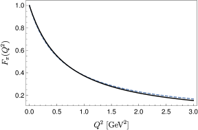
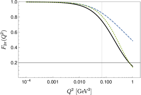
Figure 1: Left panel: the pion e.m. form factor evaluated within the lattice framework, see Eq. (22). Full black line for the configuration $A$ and dashed blue line for the configuration $B$. Right panel: comparison between the lattice eff (23) (full black line) and its approximation (24) (dashed blue line). Dotted green lines stand for the approximation (24) evaluated in the IMF, see Eq. (25).

4 The pion dPDF within the holographic QCD

In this section, details on the constituent quark models adopted to investigate basic feature of pion dPDF will be presented. In particular, we are interested in the mesonic wave function calculated by using different Light-Front holographic QCD models. The first w.f. described in this section has been introduced in Ref. [32]. The pion dPDF has been evaluated for the first time within this model in Ref. [20]. However, since the aim of this analysis is to provide a first comparison with lattice data, the pion wave function has been also evaluated by improving that of Ref. [32]. To this aim, we also considered the model where dynamical spin effects have been taken into account  [42]. In addition, in order to include other fundamental phenomenological effects, such as the Regge trajectory of the $x$-dependence of PDFs, the model of Ref. [34] has been also adopted.

4.1 Pion in AdS/QCD I: The original version

In this section, we discuss the calculation of the pion dPDF evaluated within the model described in Refs. [32, 33]. Since the w.f. obtained in this scenario can be considered as the starting point for any further implementations, here and in the following, we refer to it as the “original” model. Indeed, it can reproduce basic properties of the meson spectroscopy and structure functions. In momentum space representation, the pion wave function reads [32]:

$$\psi_{\pi o}(x,{\bf k_{1\perp}})\propto{4\pi\over\kappa_{o}\sqrt{x(1-x)}}e^{-{{\bf k^{2}_{1\perp}}\over x(1-x)2\kappa^{2}_{o}}}~{},$$ (29)

being $\kappa_{o}=0.548$ GeV fixed to reproduce the Regge behaviour of the mass spectrum of mesons. Moreover, in order to include a dependence on the quark masses, the wave function has been written in terms of the invariant mass [33]:

$$M^{2}=\sum_{i}{m_{i}^{2}+{\bf k_{i\perp}}^{2}\over x_{i}}={m^{2}+{\bf k_{1\perp}}^{2}\over x(1-x)}~{},$$ (30)

where $m=m_{1}\sim m_{2}$, $x=x_{1}$, $x_{2}=1-x_{1}$ and ${\bf k_{2\perp}}=-{\bf k_{1\perp}}$. In this scenario the pion wave function now reads:

$$\psi_{\pi o}(x,{\bf k_{1\perp}})=A_{o}{4\pi\over\kappa_{o}\sqrt{x(1-x)}}e^{-{{\bf k^{2}_{1\perp}}+m_{o}^{2}\over x(1-x)2\kappa^{2}_{o}}}~{}.$$ (31)

The mass parameter is usually chosen to be $m_{o}\sim 0.33$ GeV  [63]. The constant $A_{o}$ is fixed by the following normalisation condition:

$$\int_{0}^{1}dx~{}\int{d^{2}{\bf k_{1\perp}}\over 16\pi^{3}}|\psi_{\pi o}(x,{\bf k_{1\perp}})|^{2}=1~{}.$$ (32)

Within this approach the dPDF expression for the pion can be analytically found [20]:

$$f_{2}^{\pi O}(x,{\bf k_{\perp}})=A_{o}^{2}e^{-{4m_{o}^{2}+k_{\perp}^{2}\over 4\kappa_{o}^{2}x(1-x)}}~{}.$$ (33)

4.2 Pion in AdS/QCD II: Dynamical spin effects in holographic QCD

In Ref. [42], dynamical spin effects have been included into the holographic pion wave function in order to predict the mean charge radius of the pion and its ff without including high Fock states in the meson expansion (2). To account these contributions, let us promote the function appearing in Eq. (31) as an helicity dependent quantity, i.e.

$$\psi_{\pi s}(x,{\bf k_{\perp}})=S_{h\bar{h}}(x,{\bf k_{\perp}})\psi_{\pi o}(x,{\bf k_{\perp}})~{}.$$ (34)

Without going into details, let us discuss only the main outcomes of Ref. [42]. The spin operator reads:

$$S_{h\bar{h}}(x,{\bf k_{\perp}})=\left[Am_{\pi}^{2}+B\left({m_{o}m_{\pi}\over x(1-x)}\right)\right](2h)\delta_{-h\bar{h}}+B\left[{m_{\pi}k_{\perp}e^{i(2h)\theta_{k_{\perp}}}\over x(1-x)}\right]\delta_{h,\bar{h}}~{},$$ (35)

where ${\bf k_{\perp}}=k_{\perp}e^{i\theta_{k_{\perp}}}$. The original model, described in the previous section is restored for $B=0$ and $A=1/m_{\pi}^{2}$, i.e.:

$$\left\{\begin{array}[]{l}S_{h\bar{h}}(x,{\bf k_{\perp}})\underset{B=0}{\overset{A=1/m_{\pi}^{2}}{\longrightarrow}}{1\over\sqrt{2}}(2h)\delta_{-h\bar{h}}\\ \\ \underset{h,\bar{h}}{\sum}|S_{h\bar{h}}|^{2}=1\end{array}\right.$$ (39)

Where the last condition ensures the normalisation of the pion wave function. Let us call the dPDF evaluated within the present model, $f_{2}^{\pi AB}$, where $A$ and $B$ can assume different values. By following Ref. [42], we consider two configurations, i.e. $A=B=1$ and $A=0,~{}B=1$. In particular, the w.f. entering Eq. (34) is the same of that obtained within the original model discussed in the above section, see Eq. (31). However, in order to recover phenomenological predictions, the parameter entering the w.f. Eq. (31) is $\kappa_{0}=0.523$ GeV [42]. Also in this case, analytic expressions for dPDFs can be found:

$$f_{2}^{\pi 11}(x,{\bf k_{\perp}}) =\frac{0.0415248}{x^{2}(1-x)^{4}}e^{\frac{0.91398~{}{k^{2}_{\perp}}+0.39813}{x(x-1)}}\left.\Big{[}-12.7551~{}{k^{2}_{\perp}}(1-x)^{2}+x^{6}-4x^{5}\right.$$ (40)

$$\left.-12.6698x^{4}+52.0095x^{3}-49.4534x^{2}\right.\left.+7.5576x+5.55612\right.\Big{]}~{},$$

for the case where $A=B=1$ and

$$f_{2}^{\pi 01}(x,{\bf k_{\perp}}) =-\frac{0.64739}{(x-1)x^{2}(x-1)^{3}}e^{\frac{0.91398~{}{k^{2}_{\perp}}+0.39813}{x(x-1)}}\left.\Big{[}0.91398~{}{k^{2}_{\perp}}(1-x)^{2}+x^{4}-3x^{3}\right.$$ (41)

$$\left.+2.60187x^{2}-0.203741x-0.39813\right.\Big{]}~{},$$

for the case where $A=0$ and $B=1$. Here and in the following we refer to this model as the “dynamical spin model”.

4.3 Pion in AdS/QCD III: A universal wave function

In this last part of this section, a new and promising pion wave function, obtained from the holographic correspondence, will be presented  [34]. In this case, the basic idea is to consider the most general analytic structure of GPDs, obtained within holographic QCD, and then incorporate the Regge trajectories for small $x$ in PDFs. In this procedure, the mathematical structure preserves the poles of the ff in the physical region. Here and in the following we indicate this model as the “Universal model” (UM). Let us here just remind the main outcomes of Ref. [34]. Within this model, the effects of two Fock states in the hadron expansion (2) are considered: the valence configuration $|q\bar{q}\rangle$ and the $|q\bar{q}q\bar{q}\rangle$ contribution. These two different states are addressed with the index $\tau=2$ and $\tau=4$, respectively. A remarkable result shown in   [34] is that nucleon and pion PDFs, GPDs and ffs can be described within the same model. Of course, free parameters are chosen to describe ffs, PDFs and hadron spectroscopy at the same time. The w.f., related to a given $\tau$ state can be effectively expressed as follows:

$$\psi^{\tau}_{eff}(x,{\bf k_{\perp}})=8\pi\dfrac{\sqrt{q_{\tau}(x)f(x)}}{1-x}Exp{\left[\dfrac{2f(x)}{(1-x)^{2}}{\bf k_{\perp}^{2}}\right]}~{},$$ (42)

where here $q_{\tau}(x)$ is the $\tau$ contribution to the pion PDF. The analytical structure of this quantity is fixed by the holographic QCD approach:

$$q_{\tau}(x)=\dfrac{1}{N_{\tau}}\big{[}1-w(x)^{\tau-2}\big{]}w(x)^{-\frac{1}{2}}w^{\prime}(x)~{},$$ (43)

where:

$$w(x) =x^{1-x}e^{-a(1-x)^{2}}$$ (44)

$$f(x) =\dfrac{1}{4\lambda}\left[(1-x)\log\left(\dfrac{1}{x}\right)+a(1-x)^{2}\right]$$ (45)

$$N_{\tau} =\sqrt{\pi}\Gamma(\tau-1)/\Gamma(\tau-1/2)~{}.$$ (46)

Thanks to this choice the Regge trajectory is correctly reproduced. Moreover, the parameters $a$ and $\lambda$ have been phenomenologically fixed by fitting the mesonic mass spectrum and the e.m. form factor. Results are found for $a=0.531$ and $\kappa=\sqrt{\lambda}=0.548$ GeV. In Ref. [34], the authors fixed the weight of the two Fock states, $\gamma$, contributions by using the pion moment of PDFs:

$$f_{1}^{\pi U}(x)=(1-\gamma)q_{\tau=2}(x)+\gamma q_{\tau=4}(x)~{}.$$ (47)

In particular $\gamma=0.125$ [34]. Let us point out that the wave function of the $\tau=4$ state is computed only to calculate PDFs. Thus, the dependence of the latter upon the other two particle momenta is integrated out. Thanks to all these ingredients, the pion dPDF, $f_{2}^{\pi U}(x,k_{\perp})$, can be evaluated. In the next section numerical results will be discussed. Let us mention that this model represents an important improvements w.r.t. the original one. Indeed, in this scenario the Regge behaviour at small $x$ has been properly included together with pole structure of the form factor. In addition, let us remark that a contribution of higher Fock states to the hadron PDF has been effectively incorporated. As it will be discussed later on, such a feature is quite relevant in the present analysis.

5 Numerical Results

In this section, numerical results of the calculations of dPDFs, within holographic models, will be presented. In particular, we will mainly focus on quantities which allows to qualitatively estimate the impact of non perturbative double parton correlations, not directly accessible via one-body distributions.

5.1 Calculation of dPDFs

In the left panel of Fig. 2, Fig. 3 and the left panel of Fig. 4, we show the calculations of the pion dPDFs  (6) for fixed different values of $k_{\perp}$. In the cases of the original and dynamical spin models, the shape of these quantities are symmetric, reflecting the symmetry between $x$ and $1-x$, see left panel of Fig. 2 and Fig. 3. The different behaviour, observed in the case of the universal model, is related to the implementation of the Regge trajectory at small $x$. A common feature shared by all these models is the decreasing shape w.r.t. the increasing of $k_{\perp}$. Such a result is directly related to the behaviour of the relative eff. Details on the evaluation of the latter quantity are presented later on this section. As shown for the proton case  [14, 55], the impact of DPCs effects is enhanced for dPDFs depending on $x_{1}-x_{2}$ with $x_{1}$ and $x_{2}$ which are almost independent and bound by $x_{1}+x_{2}\leq 1$. However, for a meson, where only the two body Fock state contribution is considered in Eq. (2), the dPDF depends only on $x_{1}=x$ and $x_{2}=1-x$ due to momentum conservation  [20]. For the moment being, a full expression for the LF wave function corresponding to, e.g. a $|q\bar{q}q\bar{q}\rangle$, is not available. In fact, let us remind that, in the UM, such a contribution is included only to describe PDFs, thus a possible non trivial dependence of the dPDF on $x_{1},~{}x_{2}$ and $x_{3}$ is not addressed. In this scenario, the most relevant sign of DPCs is given by studying the $x-k_{\perp}$ dependence of dPDFs. In particular, an unfactorized dependence of dPDFs, w.r.t. the $x$ and $k_{\perp}$, represents a possible signals of double parton correlations. We recall here that in order estimate the impact of these effects, the ratio $f_{2}^{\pi}(x,k_{\perp})/f_{2}^{\pi}(x=0.4,k_{\perp})$ is evaluated as a function of $x$ for different values of $k_{\perp}$. One should notice that if correlations were neglected, then the latter quantity would be constant w.r.t. variations of $k_{\perp}$. As one can see in the right panel of Fig. 2 and in Fig. 5, correlations are very strong for the original and dynamical spin models. However, as one can observe in the right panel of Fig. 4, the impact of DPCs, encoded in the UM, is less relevant w.r.t. the other models. This feature is related to the poor general knowledge of these effects. In any case, for all models here considered, the factorisation in the $k_{\perp}$ and $x$ dependence is not fully supported.

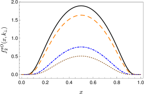
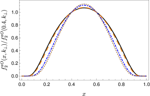
Figure 2: Left panel: dPDFs evaluated within the original model [32] and addressed for different values of $k_{\perp}$. Full black line $k_{\perp}=0$ GeV, dashed orange line $k_{\perp}=0.2$ GeV, dot-dashed blue line $k_{\perp}=0.5$ GeV and dotted brown line $k_{\perp}=0.6$ GeV. Right panel: same of the left panel for the ratio Eq. (7).

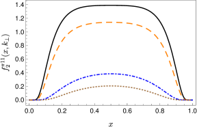
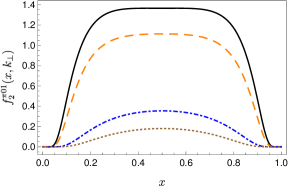
Figure 3: Double PDFs of the pion evaluated within the dynamical spin effects model [42] for different values of $k_{\perp}$. Full black line $k_{\perp}=0$ GeV, dashed orange line $k_{\perp}=0.2$ GeV, dot-dashed blue line $k_{\perp}=0.5$ GeV and dotted brown line $k_{\perp}=0.6$ GeV. Left panel for the $A=B=1$ configuration. Right panel for the $A=0,~{}B=1$ configuration.

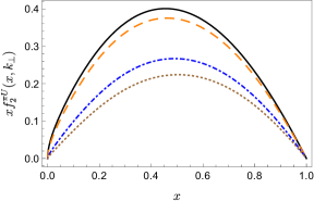
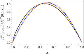
Figure 4: Same of Fig. 2 but for the universal model of Ref. [34]. In the left panel, the quantity $xf_{2}^{\pi U}(x,k_{\perp})$ is plotted.

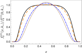
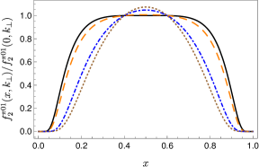
Figure 5: The ratio $r_{k}(x,k_{\perp})$, Eq. (7) evaluated for for different values of $k_{\perp}$. Full black line $k_{\perp}=0$ GeV, dashed orange line $k_{\perp}=0.2$ GeV, dot-dashed blue line $k_{\perp}=0.5$ GeV and dotted brown line $k_{\perp}=0.6$ GeV. Left panel for the $A=B=1$ configuration. Right panel for the $A=0,~{}B=1$ configuration.

5.2 The pion form factor

Since the main purpose of the present study is to compare lattice data with holographic quark model calculations, here we show results for the pion e.m. form factor. This quantity has been extensively investigated from a theoretical and experimental point of view [19, 32, 34, 42, 64]. To this aim, we consider the pion ff evaluated within the lattice techniques in the $A$ configuration. As one can see in the left panel of Fig. 6, the AdS/QCD approach is able to reproduce the essential behaviour of the pion ff. In particular, the original model [32] fits the ff in the small $Q^{2}$ region, while the dynamical spin and universal ones [34, 42] provide an impressive agreement. However, by comparing the values of the mean pion radius, one can conclude that the model which includes dynamical spin effects reproduce very well experimental data [65], see Table 1.

	Original	Dynamical Spin	Universal	Lattice	Lattice	Experiment
	model	$A=B=1$	model	(A)	(B)	[65]
$\sqrt{\langle r^{2}\rangle}$ [fm]	0.524	0.673	0.644	0.600	0.621	0.67 $\pm 0.01$

Table 1: Values of the pion mean radius, Eq. (26), obtained within the lattice and the models based on the the AdS/QCD approach. Experimental data are from Ref. [65].

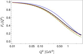
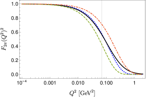
Figure 6: Left panel: the pion form factor evaluated within the lattice framework (full black line), the original model (dotted blue line), the dynamical spin model (dashed green line), in the $A=B=1$ configuration, and the universal model (dot-dashed red line). Right panel, same of the left panel for the square of the eff $F_{2\pi}(Q^{2})^{2}$.

5.3 The effective form factor of the pion

Here we show the first comparison between the calculations of the eff within AdS/QCD inspired models and that from lattice QCD, see Eq. (23). Let us first discuss some differences between the pion ff and eff. As discussed in Refs. [8, 50], in the proton case, the two objects are completely different. In particular the eff involves two particle correlations and depends on $k_{\perp}$, i.e. the momentum unbalance between the first and the second parton in the initial and final states. In the e.m. form factor, $q_{\perp}$ represents the exchanged momentum between the initial and final state of a given parton. However, in the mesonic case, if one considers only the $|q\bar{q}\rangle$ contributions, the formal expression of the eff (9) and the e.m. (15) one are extremely similar (see Ref. [20] for details on this topic). In addition, $k_{\perp}$ represents the conjugate variable to $d_{\perp}$, i.e. the transverse distance between the two partons, while $q_{\perp}$ is the conjugate variable to $r_{\perp}$, i.e. the transverse distance of a parton w.r.t. the centre of the hadron. In the right panel of Fig. 6, results of the calculations of $F_{2\pi}(Q^{2})^{2}$ has been shown. We remind that this combination of two effs enters the expression of $\overline{\sigma}_{eff}$, see Eq. (17), and encodes the hadron geometrical properties which affect this experimental observable. Thus, in the right panel of Fig. 6, we highlighted the main discrepancies, between lattice and model calculations, which also affect the mean value of $\sigma_{eff}$. As one can see, only the original model is able to reproduce the eff in the allowed kinematic region. Let us stress again that the comparison is well motivated only for $Q^{2}<m_{\pi}^{2}$. In the forward region, frame dependent effects are important but not included in the LF formalism. It is fundamental to point out that, while in the lattice framework there are no truncation of the meson Fock state, in all AdS/QCD models, but the UM one, only the first $|q\bar{q}\rangle$ contribution is included. Thus the dPDF is restricted to be considered as an unintegrated PDF where the momentum conservation unambiguously fixes the relation between $x_{1}$ and $x_{2}=1-x_{1}$. In this scenario, lattice data of the first moment of dPDFs of the pion represent a reach starting point to understand in details the contribution of high Fock states in the meson expansion Eq. (2). Thanks to this analysis, further implementations of holographic models could include two-body effects based on the lattice data [19]. As one can see in Table 2, the lattice calculation of $\langle d^{2}\rangle$ is comparable to that obtained within the original model. On the contrary, the UM largely underestimates the mean partonic distance.

	Original	Dynamical Spin	Universal	Lattice
	model	$A=B=1$	model	(A)
$\sqrt{\langle d^{2}\rangle}$ [fm]	0.968	1.207	0.767	1.046 $\pm 0.049$

Table 2: Values of the 3D mean partonic distance in the pion, Eq. (19), obtained within the lattice and the model based on the the AdS/QCD approach.

5.4 Calculation of $\overline{\sigma}_{eff}$

Here we discuss a possible prediction for an ideal DPS process involving two pions. Due to the lack of data and experimental analyses, we focus on the mean value $\sigma_{eff}$ (17). In this scenario, only geometrical properties affecting $\sigma_{eff}$ have been taken into account. The evaluation of this quantity within the lattice framework would be extremely valuable in order to guide future experimental analyses. However, as extensively discussed in the previous sections, lattice data have been obtained in the pion rest frame. Therefore a direct phenomenological prediction cannot be safely obtained. However, one can evaluate the mean value of $\sigma_{eff}$ by changing the higher extreme value of the integral in Eq. (17). In fact, for $k_{\perp}<m_{\pi}$, frame dependent effects are small. For the purpose of the present investigation, in Table 3, we have reported the results of the calculations of $\overline{\sigma}_{eff}$. As one can observe in the first row, up to $m_{\pi}$, the original model predicts a $\overline{\sigma}_{eff}$ very close to that obtained from the lattice. Let us remind that the full value of $\overline{\sigma}_{eff}$, evaluated within this model, has been used in the experimental analysis of Ref. [60]. This result is completely coherent with the comparison between the eff evaluated within the lattice QCD and the original model. From just a mathematical point of view, we also displayed the calculation of $\overline{\sigma}_{eff}$ in the full range of $k_{\perp}$. As one can observe, the universal model provides a good fit with lattice results. However, let us stress again that in this case, frame dependent effects, preventing a clear comparison between lattice and holographic calculations, cannot be neglected. The full evaluation of $\sigma_{eff}$ is anyhow relevant to verify the validity of the RC inequality (20). As one can observe in Table 4, the latter perfectly works for all models and lattice calculations. Let us stress again that the relation between the mean value of $\sigma_{eff}$ and the mean distance between two partons has been obtained in a complete general manner in Ref. [9]. Therefore, the validation of the RC inequality, in model independent frameworks, such as the lattice QCD, is extremely precious.

	Original	Dynamical Spin	Dynamical Spin	Universal	Lattice
	model	$A=B=1$	$A=0,~{}B=1$	model
$\overline{\sigma}_{eff}^{0~{}\mbox{to}~{}m_{\pi}}$ [mb]	76.2	89.4	90.7	67.3	77.7
$\overline{\sigma}_{eff}$ [mb]	38.3	60.9	62.6	22.2	26

Table 3: Values of $\overline{\sigma}_{eff}$ obtained within different pion models and the lattice approach, by taking into account only geometrical effects. In the first row $\overline{\sigma}_{eff}$ has been evaluated by performing the integral in Eq. (17) from $0$ to $k_{\perp}\sim m_{\pi}$. In the second row, the full calculation of $\overline{\sigma}_{eff}$ has been performed.

Model	$\sqrt{\dfrac{\overline{\sigma}_{eff}}{3\pi}\dfrac{3}{2}}$	$\sqrt{\langle d^{2}\rangle}$	$\sqrt{\dfrac{\overline{\sigma}_{eff}}{\pi}\dfrac{3}{2}}$
	[fm]	[fm]	[fm]
Original	0.781	0.968	1.352
Dynamical Spin	0.980	1.207	1.697
Universal	0.594	0.767	1.029
Lattice	0.647	1.046	1.121

Table 4: Check of the validity of the RC inequality (20) in 3-dimension.

5.5 Comparison between two-body distributions and the product of one-body functions

In this last part of this section, devoted to the study of the pion dPDFs, we discuss the validity of Eqs. (12) and (13). Let us start with the comparison between $f_{2}^{\pi}(x,{\bf k_{\perp}})$ and its approximation $f_{2,A}^{\pi}(x,{\bf k_{\perp}})$, i.e. the product of the pion GPD and its form factor, see Eq. (12). Since the dPDFs of nucleons and mesons are basically unknown, in order to estimate the magnitude of DPS cross section, the approximation (10) is often used. In this framework, model calculations can be used to test the validity of this ansatz. Here we consider the same strategy developed in Ref. [20], i.e. we directly compare $f_{2}^{\pi}(x,{\bf k_{\perp}})$ and $f_{2,A}^{\pi}(x,{\bf k_{\perp}})$ by remarking their differences. In Figs. 7 and 8, distributions have been evaluated for three different values of $k_{\perp}$ as functions of $x$. As one can see, in all model calculations, but the UM case, the shape of dPDFs is symmetric, at variance of the product of ffs and GPDs. Such a feature can be explained by considering that GPDs and form factors depend on the transverse momentum: ${\bf k_{1,\perp}}\pm(1-x){\bf k_{\perp}}$, see Eq. (15). Such a dependence, produces an asymmetry in the $x$ distribution, not present in dPDF, see Eq. (6). Moreover, since in the GPDs the momentum unbalance in the wave function is multiplied by the pre-factor $1-x<1$, the GPD goes to zero slower then the dPDF [20]. The last feature is partially discussed in Ref. [9] for the proton case. Furthermore, one should notice, that for the original and dynamical spin models the approximation Eq. (12) underestimates the full calculation of the dPDF, at the variance of the universal case. In order to compare the impact of DPCs described within the lattice QCD and holographic models, the following quantity will be also evaluated:

$$\Delta(Q^{2})=F_{2\pi}(Q^{2})-F_{\pi}(Q^{2})^{2}~{}.$$ (48)

In order to minimise frame dependent effects, we will focus on the region where $Q^{2}<m_{\pi}^{2}$. As one can see, if the approximation Eq. (13) holds in some kinematic region, then the above quantity would be small. In Fig. 9 the calculations of the $\Delta(Q^{2})$ function are displayed. As one can observe, in the allowed region of $Q^{2}$, the original and dynamical spin models can almost reproduce the behaviour of DPC effects. In any case, one should notice that there is no model able to reproduce both the effective and the e.m. form factors at the same time with the same precision. In fact, both the dynamical spin and universal models, fit very well data on the e.m. form factor but fail in the description of the eff. On the contrary, the original model can qualitatively reproduce both the effective and e.m. form factors only in the small $Q^{2}$ region. The main outcome of this analysis is the evident need of the inclusion of more Fock states in the pion expansion (2) necessary to include all possible DPCs in order to describe both the e.m. and effective form factors. Let us stress that since the universal model effectively takes into account the $|q\bar{q}q\bar{q}\rangle$ state, it is suitable to deeply investigate the impact of non trivial DPCs in the pion. Further studies on the top of that, beyond the present analysis, are on going.

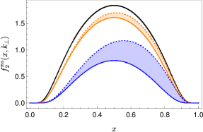
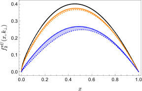
Figure 7: Full lines represent the pion dPDF Eq. (6) and dotted lines stand for the approximation Eq. (12). Quantities are evaluated for three values of $k_{\perp}$: $k_{\perp}=0$ GeV black lines, $k_{\perp}=0.2$ GeV orange lines and $k_{\perp}=0.5$ GeV blue lines. The bands stand for the difference between the full calculation of the dPDF and its approximation. Left panel for the original model of Ref. [32]. Right panel for the UV of Ref. [34].

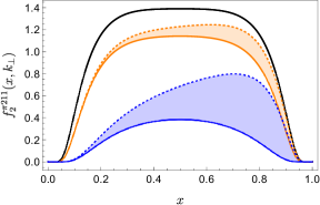
Figure 8: Same of Fig. 7 but for the dynamical spin model of Ref. [42]. Left panel for the configuration $A=0,~{}B=1$. Right panel: for the configuration $A=B=1$.

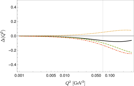
Figure 9: The quantity $\Delta(Q^{2})$ (48). Full black line stands for lattice data [19], dotted yellow line for the calculation performed within the universal model [34], dashed green line represent the result of the evaluation within the original model [32] and dot-dashed red for the dynamical spin model [42] in the $A=B=1$ configuration.

5.6 Parameter dependence of the results

In this final section about the pion target, a short discussion about the parameter dependence of the main results will be presented. In particular the form factor, the eff and the function $\Delta(Q^{2})$ will be evaluated by changing the model parameters in order to improve the agreement with lattice data.

5.6.1 The Original model

As already mentioned, the the meson wave function evaluated within this model depends on two parameter $\kappa$ and $m_{0}$. Indeed, as shown in Ref. [27] the value of $\kappa$ smoothly depends on the observable one needs to fit. In fact, $\kappa$ obtained from the form factor is basically smaller then that obtained by fitting the spectrum. In particular, $\kappa$ lies in the range $0.35\leq\kappa\leq 0.59$ GeV. Therefore here we present a selected collection of results, previously shown, as functions of $\kappa$. As one can see Fig. 10, the variation on $\kappa$ could allow to provide a good description of the form factors and the eff. Therefore, a good agreement with lattice data could be obtained by adding a theoretical error on $\kappa$. One can interpret such an uncertainty as an attempt to include two-body effects in the wave function of the first Fock state. In this scenario, the mean radius and the main distance read: $\sqrt{\langle r^{2}\rangle}=0.625\pm 0.135$ fm and $\sqrt{\langle d^{2}\rangle}=1.17\pm 0.28$ fm, respectively. The lattice and experimental results are included into the found ranges. Moreover, as one can see in Fig. 11, the double parton correlations, emphasised by the function (48), are well reproduced. However the changes in $\kappa$ will produce modifications of the PDFs and a different description of the spectrum.

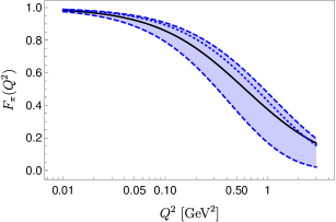
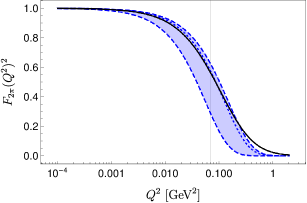
Figure 10: Left panel: the pion form factor evaluated with the original model. The band stands for the results obtained by varying $\kappa$: $0.35\leq\kappa\leq 0.59$ GeV. Dotted lines represents the result for $\kappa=0.548$ GeV. Right panel: same of the left panel for the quantity $F_{2\pi}(Q^{2})^{2}$.

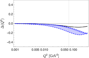
Figure 11: The function Eq. (48) evaluated with the original model. The band stands for the results obtained by varying $\kappa$: $0.35\leq\kappa\leq 0.59$ GeV.

5.6.2 The Universal model

In the case of this model, use has been made of different parameters in order to properly fit several observable, i.e. $a,\lambda$ and $\gamma$, see Eqs. (43,44) and (45). In Figs. 12 and 13, the previous calculations of the form factor, eff, PDF and $\Delta$ will be compared with those obtained within another choice of the parameters, i.e. $a=1.4,~{}\sqrt{\lambda}=0.51$ GeV and $\gamma=0.01$. As one can see in Fig. 12, within this combination, both the form factor and the eff qualitatively reproduce the lattice data. The function $\Delta(Q^{2})$ is also closer to that evaluated within the lattice QCD w.r.t. that shown in Fig. 9. However, as one can see in the right panel of Fig. 13, the price for this choice of the parameters is a relevant change of the shape of the PDF. Therefore one might expect a relevant loss of agreement between PDF data and model calculations; in particular in the high $x$ region. Since one of the motivation for the choice of original values of $a,\lambda$ and $\gamma$ is also the excellent fit with PDF [34], one might conclude that a good strategy to explain lattice data, on DPCs, would be a further study on higher Fock states in the meson expansion. In this scenario, the universal model is potentially very promising being the only one which effectively includes the $\bar{q}qq\bar{q}$ contribution. A detailed investigation on the LF wave function $\psi_{\bar{q}qq\bar{q}}$ guided by these lattice data would open a new window on the meson structure.

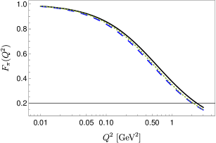
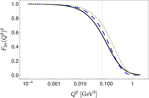
Figure 12: Left panel: the pion form factor evaluated with the universal model. The blue dashed lines represent the calculation obtained by setting $a=1.4,~{}\sqrt{\lambda}=0.51$ GeV and $\gamma=0.01$. Dotted lines represents the result for the standard values of the parameters $a,~{}\lambda$ and $\gamma$, see Sect. 5.6.2 for details. Right panel: same of the left panel for the quantity $F_{2\pi}(Q^{2})^{2}$.

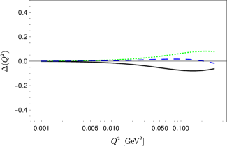
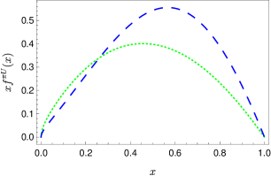
Figure 13: Same of Fig. 12 but left panel: for the $\Delta(Q^{2})$ function. Right panel: for the pion PDF.

6 The $\rho$ meson within AdS/QCD

In this section, we introduce and calculate the dPDFs of the $\rho$ meson. This is the first analysis of DPS involving a vector meson. However, in the future moments of the $\rho$ dPDFs could be accessed via lattice techniques. Here we consider possible predictions provided by AdS/QCD based models. In order to evaluate the $\rho$ w.f., the procedure developed in Refs. [35, 66, 67] has been adopted. In particular, for the three polarisation of the $\rho$ meson, the wave function is built from that of the pion. In this case, the input will be the w.f. Eq. (31). In this case, the normalisation constant will depend on the $\rho$ polarisation. In Ref. [67] the parameters have been chosen to describe several observable for both the $\rho$ and the $\phi$ mesons. In particular $\kappa_{o}=0.54$ GeV and $m_{o}=0.14$ GeV (configuration A). In the present work we propose and motivate the use of another combination of the parameters. In particular those used to calculate the pion w.f. (31), i.e. $\kappa_{0}=0.548$ and $m_{o}=0.33$ GeV (configuration B), will be considered. A detailed analysis on this choice will be provided. Let us mention that a good comparison with the moments of $\rho$ PDFs, evaluated within the lattice QCD, is obtained within the B configuration. The $\rho$ w.f., built from that of the pion, reads as follows:

$$\Psi^{L}_{h,\bar{h}}(x,b_{\perp})={1\over 2}\left(1+{m_{f}^{2}-\bigtriangledown^{2}\over m_{\rho}^{2}x(1-x)}\right)\phi_{L}(x,\zeta)\delta_{h,\bar{h}}$$ (49)

$$\Psi^{T=\pm}_{h,\bar{h}}(x,b_{\perp})=\pm\Big{[}ie^{\pm i\theta}\Big{(}x\delta_{\pm h,\mp\bar{h}}-(1-x)\delta_{\mp h,\pm\bar{h}}\Big{)}\partial_{b_{\perp}}+m_{f}\delta_{\pm h,\pm\bar{h}}\Big{]}{\phi_{T}(x,\zeta)\over 2x(1-x)}~{}.$$ (50)

Where here and in the following, we denote with $\Psi^{\lambda}_{h,\bar{h}}(x,b_{\perp})$ the $\rho$ meson wave function in coordinates space for $\lambda=L,T$ polarisation and quark-antiquark helicities $h$ and $\bar{h}$, respectively. Moreover, $\zeta$ is the usual variable introduced in the AdS/QCD framework, i.e. $\zeta=\sqrt{x(1-x)}b_{\perp}$. The symbol $\bigtriangledown^{2}\equiv{1\over b_{\perp}}\partial_{b_{\perp}}+\partial^{2}_{b_{\perp}}$. The gaussian like function, appearing in Eqs.(49, 50), describes the scalar part of the meson w.f. in AdS/QCD (31):

$$\phi_{\lambda}(x,\zeta)=N_{\lambda}\sqrt{x(1-x)}e^{-{\kappa_{o}^{2}\zeta^{2}\over 2}}e^{-{m_{o}^{2}\over 2\kappa_{o}^{2}x(1-x)}}~{}.$$ (51)

In Eq. (50), $b_{\perp}e^{i\theta}$ is the complex form of the vector ${\bf b_{\perp}}$. The normalisation condition of the $\rho$ w.f. is the following:

$$\sum_{h,\bar{h}}\int dx~{}d^{2}{\bf b_{\perp}}~{}\big{|}\Psi^{\lambda}_{h,\bar{h}}(x,b_{\perp})\big{|}^{2}=1~{}.$$ (52)

The normalisation constant, $N_{\lambda}$ appearing in Eq. (51), depends on the polarisation [35]. From the above expressions, the dPDF for a given polarisation can be obtained as follows:

$$f_{2}^{\rho,\lambda}(x,k_{\perp}) =\sum_{h,\bar{h}}\int d^{2}{\bf b_{\perp}}e^{i{\bf k_{\perp}}\cdot{\bf k_{\perp}}}\big{|}\Psi^{\lambda}_{h,\bar{h}}(x,b_{\perp})\big{|}^{2}=2\pi\sum_{h,\bar{h}}\int db_{\perp}~{}b_{\perp}J_{0}(b_{\perp}k_{\perp})\big{|}\Psi^{\lambda}_{h,\bar{h}}(x,b_{\perp})\big{|}^{2}~{}.$$

In the transverse polarisation case, since dPDFs are diagonal distributions in coordinate space, the main quantity we need to evaluate is the following one:

$$\sum_{h,\bar{h}}\big{|}\Psi^{T}_{h,\bar{h}}(x,\zeta)\big{|}^{2}={|\phi_{T}(x,\zeta)|^{2}\over 4x^{2}(1-x)^{2}}\Big{[}2m_{f}^{2}+\kappa_{\rho}^{4}\zeta^{2}x(1-x)(x^{2}+(1-x)^{2})\Big{]}~{}.$$ (53)

6.1 Numerical results

Here we show the numerical predictions for the dPDFs and effs of the $\rho$ mesons. Since this is the first analysis about this topic, the $\rho$ moments of PDFs have been used to motivate the choice of the free parameters appearing in Eq. (51). To this aim, we compare the calculations of these quantities, obtained within the AdS/QCD approach, with those addressed by the lattice QCD  [68]. Furthermore, also for this hadron, the role of DPCs in dPDFs and in effs will be investigated. In addition, we have also calculated the mean value of $\sigma_{eff}$ in order to provide a first prediction for this experimental quantity. Thus, for the moment being, only the geometrical contributions have been taken into account in the meson $\sigma_{eff}$.

6.2 The parameters entering the $\rho$ wave functions

In Refs. [35, 66, 67] the parameters appearing in Eq. (51) have been properly chosen to reproduce the diffractive cross section for the $\rho$ and $\phi$ meson productions. Within the A configuration, also the decay constants are well reproduced. In the present analysis, we propose to use the parameters of the B configuration, in order to have a good agreement with lattice data of the $\rho$ moments of PDFs. To this aim, we first show the different predictions for the decay constants, obtained within different combination of the two free parameters $\kappa$ and $m_{0}$. We consider the following expressions:

$$f_{\rho} =\sqrt{\dfrac{N_{c}}{\pi}}\int_{0}^{1}dx~{}\left[1+\dfrac{m_{o}^{2}-\bigtriangledown_{b}^{2}}{x(1-x)M_{\rho}^{2}}\right]\Psi^{L}(x,b)\Big{|}_{b=0}$$ (54)

$$f_{\rho}^{\perp} =\sqrt{\dfrac{N_{c}}{2\pi}}m_{o}\int_{0}^{1}dx~{}\int db~{}\mu J_{1}(\mu b)\dfrac{\Psi^{T}(x,b)}{x(1-x)}~{},$$ (55)

where $\Psi^{\lambda}(x,b)=\sum_{h,\bar{h}}\Psi^{\lambda}_{h,\bar{h}}(x,b)$, $b=|{\bf b}_{\perp}|$ and $\mu=1$ GeV. In Fig. 14, the above quantities are displayed as a function of the parameters $m_{0}$ and $\kappa$, respectively. As one can observe a good comparison with the sum rules [69, 70] is obtained for a limited choice of the parameters. Here below we compare in details the results obtained within the A and B configurations. In fact, the former leads to good comparisons with data on diffractive $\rho$ production, while in the latter the same parameters entering the original model for the pion have been used. Let us recall that the w.f. of the original model represents the dynamical input used to evaluate the $\rho$ w.f., see Eq. (51). Therefore within the B configuration the $\rho$ eff can be calculated from the pion model which better reproduce the lattice data [19] w.r.t. the other models. In addition let us mention that within the B configuration $\kappa=0.548$ GeV, i.e. the same value adopted in both the original and universal pion models, thus reflecting the universal condition for the breaking of the conformal symmetry. As one can observe in Table 5, the results of the calculations of $f_{\rho}$ and $f_{\rho}^{\perp}$, within the A and B configurations, are very similar and comparable to those of Refs. [69, 70].

Approach	Configuration	$f_{\rho}$[MeV]	$f_{\rho}^{\perp}$ [MeV]
	A	211	95
LF holography	B	204	150
Sum rules [69]		$198\pm 7$	$152\pm 9$
Sum rules [70]		$206\pm 7$	$145\pm 9$

Table 5: Predictions for the $\rho$ decay constants.

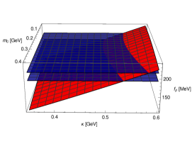
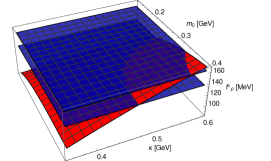
Figure 14: Left panel: the calculation of $f_{\rho}$ (54) as a function of $m_{0}$ and $\kappa$ (the red diagonal plane). The blue horizontal planes represent the uncertainty obtained from sum rules [69, 70]. Right panel: same of the left panel but for $f_{\perp}^{\rho}$ (55).

6.2.1 Comparison with lattice QCD

Here we discuss the comparison between the moments of the $\rho$ PDFs, evaluated within the holographic model  [35, 66, 67], with those obtained within the lattice QCD [68]. Let us remind that for the moment being their are no analyses of dPDF moments for the $\rho$ meson. Thus, in order to investigate to what extent the adopted model could be compared to lattice predictions, here we only consider moments of the following structure function:

$$F_{1}(x)=\sum_{q}Q_{q}^{2}\dfrac{1}{3}\Big{(}f_{1,q\bar{q}}^{\rho T}(x)+f_{1,q\bar{q}}^{\rho L\uparrow}(x)\Big{)}~{},$$ (56)

where here $q$ is the quark flavor with charge $Q_{q}$, $f_{1,q\bar{q}}^{\rho T}(x)$ is the $\rho$ PDF with transverse polarisation and $f_{1,q\bar{q}}^{\rho L\uparrow}(x)$ is the PDF of the $\rho$ meson longitudinally polarised and evaluated for a quark with positive helicity. Since, in the holographic model, the latter quantity does not depends on the spin orientation, nor the flavor of the quarks, the above structure functions can be rewritten in terms of PDFs for unpolarised quarks:

$$F_{1}(x)=\sum_{q}Q_{q}^{2}\dfrac{1}{3}\left(f_{1}^{\rho T}(x)+\dfrac{f_{1}^{\rho L}(x)}{2}\right)~{}.$$ (57)

In Ref. [68], the following quantity has been calculated:

$$a_{n}=2\int_{0}^{1}dx~{}x^{n-1}F_{1}(x)~{}.$$ (58)

As one can observe in Fig. 15, the first moment of the $\rho$ PDF is almost stable. Lattice data on $a_{2}$ and $a_{3}$ are contained inside the error bar which reflects variations of the model parameters. Further improvements of the model are beyond the purpose of the present analysis. However the other moments are well reproduced and in particular in the B configuration one gets: $a_{2}=0.161$ and $a_{3}=0.102$ which are admitted by the theoretical error of lattice data. In further analyses, implementations of the $\rho$ w.f. to improve the comparison with the lattice outcomes will be available. For example, one can use the pion wave function evaluated within the models of Refs. [34, 42] as input of the procedure.

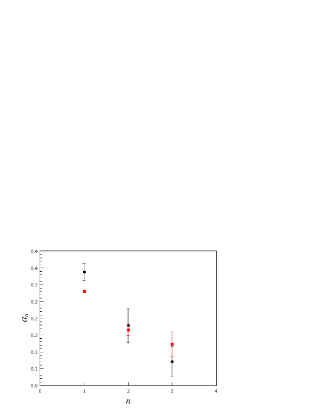
Figure 15: Calculations of moments of the $\rho$ structure function Eq. (57). Round black points for lattice results. Squared red points for model calculations obtained within the holographic model of Refs. [35, 66, 67] and including variations of $0.35\leq\kappa\leq 0.6$ GeV.

6.3 Calculations of dPDFs, effs and $\overline{\sigma}_{eff}$

In the present section, we show and discuss the results of numerical evaluations of $\rho$ dPDFs, effs and $\overline{\sigma}_{eff}$ in the B configurations of the parameters entering Eq. (51). The above quantities have been calculated for the longitudinal and transverse polarisations separately. As for the pion case, in Fig. 16, we display the $\rho$ dPDFs for the two possible polarizations: left panel for the longitudinal polarisation and right panel for the transverse one, respectively. As one might notice, the $k_{\perp}$ behaviour of the distributions is similar to that obtained for the pion evaluated within the original models, see left panel of Fig. 2. Such a result is coherent with the choice of the scalar w.f. entering Eqs. (49) and (50). Moreover, in the transverse polarisation case, the distribution has two pronounced peaks. In addition, as one can see in Fig. 17, a possible factorisation between the $x$ and $k_{\perp}$ dependence is violated, thus reflecting the presence of correlations. The amount of these effects is slightly different from those addressed in the right panel of Fig. 2 obtained within the original model. This feature is related to the presence of derivatives w.r.t. $b_{\perp}$ in Eqs. (49) and (50). Thus, the overall dependence on $k_{\perp}$ of the $\rho$ dPDFs is somehow different from that of the pion. The main interpretation of the present outcome is that the procedure, used to generate the $\rho$ w.f., introduces additional correlations. Moreover, the mean value of the effective cross section reads: $\overline{\sigma}_{eff}=27.8$ mb for the longitudinal case and $\overline{\sigma}_{eff}=54.7$ mb for the transverse one. In order to provide a proper interpretation to these results, let us remark that the original model, used as input for the above calculations (49-50), qualitatively fits the Lattice data. Therefore it is reasonable to expect that also predictions for the $\rho$ could be realistic. Thereby one can conclude that the DPS cross section is dominated by the longitudinal component of the $\rho$ meson. In fact, we recall that the most $\sigma_{eff}$ is small the most the DPS contribution is big with respect to the SPS case, see Eq. (16). In Fig. 18 the eff of the $\rho$ meson, obtained by disentangling the two polarisation contributions, is shown. Full line represents the transverse polarisation and dotted line stands for the longitudinal one. By using Eq. (19), from the eff the mean partonic distance between two partons in the $\rho$ has been calculated: $\sqrt{\langle d^{2}\rangle}=0.826$ fm and $\sqrt{\langle d^{2}\rangle}=1.159$ fm, for the longitudinal and transversal polarizations, respectively. One should notice that in the former case the mean distance is lower then that evaluated for the pion target within the same original model [32], at the variance of the transversely polarised case, see Table 1. Since, the original model predicts a mean value of $\langle d^{2}\rangle$ in agreement to that of the the lattice QCD, one might expect that valence quarks in the $\rho$ meson are closer to each other then in the pion case if the the $\rho$ is longitudinally polarised. This feature represents an extreme interesting prediction directly related to the non-perturbative structure of the $\rho$ meson. Let us also show that the RC inequality (20) perfectly works also for the $\rho$ meson described within the holographic approach, see Table 6.

$\rho$	$\sqrt{\dfrac{\overline{\sigma}_{eff}}{3\pi}\dfrac{3}{2}}$	$\sqrt{\langle d^{2}\rangle}$	$\sqrt{\dfrac{\overline{\sigma}_{eff}}{\pi}\dfrac{3}{2}}$
Meson	[fm]	[fm]	[fm]
Longitudinal polarisation	0.665	0.826	1.15
Transverse polarisation	0.933	1.58	1.62

Table 6: Check of the validity of the RC inequality (20) in 3-dimension for the $\rho$ meson.

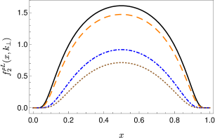
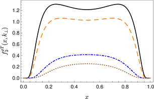
Figure 16: Same of Fig. 3 for the $\rho$ meson. Left panel for longitudinal polarisation. Right panel for transverse polarisation.

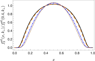
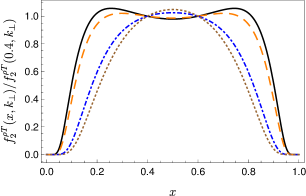
Figure 17: Same of Fig. 5 for the $\rho$ meson. Left panel for longitudinal polarisation. Right panel for transverse polarisation.

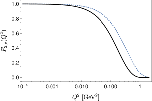
Figure 18: The effective form factor Eq. (9), evaluated for the $\rho$ system. Full black line for the transverse polarisation and dotted blue line for the longitudinal one.

7 Conclusions

Double parton distribution functions are new fundamental quantities encoding information on the three dimensional partonic structure of hadrons. Double PDFs enter the double parton scattering cross section for which theoretical and experimental analyses are ongoing. However, for the moment being, only proton-proton and proton-ion collisions are investigated from an experimental point of view. Nevertheless, lattice data on distributions related to the first moment of the pion dPDFs are now available. These quantities encode double parton correlations which cannot be accessed via one-body functions such as standard form factors. This conclusion is qualitatively coherent with the quark model analyses for the proton target. The main purpose of the present study is to compare lattice QCD predictions of the effective form factor with quark model calculations. In particular, here we have considered AdS/QCD soft-wall inspired pion models for which phenomenological implementations are also included. Double PDFs have been calculated by showing their full dependence on the longitudinal momentum fraction and the transverse momentum unbalance ${\bf k_{\perp}}$. Ratios sensitive to DPCs have been calculated and results show that DPCs are relevant. An important comparison between dPDFs and their approximations in terms of GPDs and form factors have been also investigated. Holographic model predictions shows that even if the pion is described by considering only the first $|q\bar{q}\rangle$ state, dPDFs cannot be described in terms of one-body functions. Such a conclusion is consistent with previous studies of the proton dPDFs. Let us stress here that such an approximation is largely used in phenomenological analyses of DPS processes. In order then to provide useful predictions, an estimate of the experimental observable $\sigma_{eff}$ has been provided via quark models and lattice QCD. These results have been properly interpreted in terms of geometrical properties of the pion partonic structure by verifying the RC inequality. Furthermore, moments of dPDFs, i.e. the effective form factors, have been calculated within the adopted quark models and then compared with lattice data for the first time. Despite the limited region in $Q^{2}$, which minimises the impact of frame dependent effects, one can conclude that for the moment being the absence of a complete evaluation of high Fock states in the pion expansion prevents a simultaneous description of the electric-magnetic and effective form factors. Nevertheless, the original AdS/QCD model almost matches the lattice eff and qualitatively reproduces the impact of double parton correlations. On the contrary, even if the other models provide an impressive description of the e.m. form factor, they fail in the evaluation of the eff. These first comparisons, between lattice and quark model analyses, point to the necessity of an accurate description of the contributions of high Fock states in the pion. The main conclusion is that lattice data can be used to add new constraints on future implementations of holographic models. Let us mention that for the moment being, the only model which already effectively includes a $q\bar{q}q\bar{q}$ contribution is the universal one. Therefore the latter is very promising and suitable to describe both one-body quantities and DPCs in the meson at the same time; thus shedding a new light on the parton structure of the pion. From another perspective, even if the frame dependence of the lattice eff prevents to get a phenomenological value of $\sigma_{eff}$, the RC inequality has been inverted in order to provide a range of frame independent values of $\overline{\sigma}_{eff}$ starting from the $\langle d^{2}\rangle$ addressed by lattice QCD. Such a procedure leads to a value of $\overline{\sigma}_{eff}$, for a pion-pion collision, which is bigger then to the proton-proton case. This conclusion is directly obtained from lattice QCD data and could guide future experimental and theoretical analyses. In the final part of this investigation, predictions for dPDFs and effs of the $\rho$ meson have been discussed for the first time. The main outcome of this analysis is that the impact of DPCs change with the meson polarisation.

Appendix A

In this section we discuss some details on the derivation of the dPDFs expression in terms of the LF wave function. In particular, we make use of the lattice conditions discussed in Sect. 3. Let us remind that the correlator matrix we need to evaluate is defined with quark field operators separated by a distance $y^{\mu}$ with $y^{0}=0$. Moreover, $\gamma^{0}$ is the gamma matrix considered in the dPDF correlator. In this section we show in which kinematic conditions, frame dependent effects, due to the lattice conditions, are minimised. To this aim, let us recall the main ingredients of the procedure. In particular, we have used the convention described in the Appendix A of Ref. [32]. The quark field operators, defined in terms of light-cone coordinates, reads:

$$q(x)=\sum_{\lambda}\int_{l^{+}>0}\dfrac{dl^{+}d^{2}\bf l_{\perp}}{\sqrt{2l^{+}}(2\pi)^{3}}~{}\big{[}b_{\lambda}(l)u_{q}(l,\lambda)e^{-il\cdot x}+d_{\lambda}^{\dagger}(l)v_{q}(l,\lambda)e^{il\cdot x}\big{]},$$ (59)

where the anticommutation relation for the spinors reads:

$$\big{\{}b_{\lambda}(l),b^{\dagger}_{\lambda^{\prime}}(l^{\prime})\big{\}}=\big{\{}d_{\lambda}(l),d^{\dagger}_{\lambda^{\prime}}(l^{\prime})\big{\}}=(2\pi)^{3}\delta(l^{+}-l^{\prime+})\delta^{(2)}(\bf l_{\perp}-\bf l^{\prime}_{\perp})\delta_{\lambda\lambda^{\prime}}~{}.$$ (60)

Furthermore, the one particle state is:

$$|l,\lambda\rangle=\sqrt{2l^{+}}b_{\lambda}^{\dagger}(l)|0\rangle~{},$$ (61)

with the normalisation:

$$\langle l,\lambda|l^{\prime},\lambda^{\prime}\rangle=2(2\pi)^{3}l^{+}\delta(l^{+}-l^{\prime+})\delta^{(2)}(\bf l_{\perp}-\bf l^{\prime}_{\perp})\delta_{\lambda,\lambda^{\prime}}~{}.$$ (62)

Moreover, for unpolarized dPDFs, the following relations are usually the relevant ones:

$$\bar{u}_{\downarrow}(l)\gamma^{+}u_{\downarrow}(k)=\bar{u}_{\uparrow}(l)\gamma^{+}u_{\uparrow}(k)=2\sqrt{(l^{+}k^{+})}$$ (63)

$$\bar{u}_{\downarrow}(l)\gamma^{+}u_{\uparrow}(k)=\bar{u}_{\uparrow}(l)\gamma^{+}u_{\downarrow}(k)=0,$$

where in the above equation $u_{\sigma}(k)=u_{q}(k,\sigma)$. Now, for $\gamma^{0}$ one gets:

$$\bar{u}_{\downarrow}(l)\gamma^{0}u_{\downarrow}(k)=\sqrt{(l^{+}k^{+})}+\dfrac{(l_{x}+il_{y})(k_{x}-ik_{y})}{\sqrt{l^{+}k^{+}}}$$ (64)

$$\bar{u}_{\uparrow}(l)\gamma^{0}u_{\uparrow}(k)=\sqrt{(l^{+}k^{+})}+\dfrac{(l_{x}-il_{y})(k_{x}+ik_{y})}{\sqrt{l^{+}k^{+}}}$$

$$\bar{u}_{\downarrow}(l)\gamma^{0}u_{\uparrow}(k)=-\bar{u}_{\uparrow}(l)\gamma^{0}u_{\downarrow}(k)\sim 0~{}.$$

The last relation is 0 since in the IMF the term $m/P^{+}$ can be neglected as well as for the $\gamma^{+}$ case. The first line of the above equation is similar to that obtained within the light-cone treatment case, but the main difference is the presence of the transverse components of the quark momenta. However, by using momentum conservation, Eq. (64) can be written in terms of $k^{+}=P^{+}x_{1}$ and $l^{+}=\bar{x}_{1}P^{+}$:

$$\sqrt{l^{+}k^{+}}+\dfrac{(l_{x}+il_{y})(k_{x}-ik_{y})}{\sqrt{l^{+}k^{+}}}=P^{+}\sqrt{x_{1}\bar{x}_{1}}+\dfrac{(l_{x}+il_{y})(k_{x}-ik_{y})}{P^{+}\sqrt{x_{1}\bar{x}_{1}}}~{}.$$ (65)

Since, by using the standard LF procedure discussed in Sect. 2, the dPDF does not depends on the meson frame, the $P^{+}$ dependence is completely simplified. Such a procedure leads to rewrite the correction due to the choice of $\gamma^{0}$ as follows:

$$\mathcal{O_{\gamma}}\propto\dfrac{(l_{x}+il_{y})(k_{x}-ik_{y})}{(P^{+})^{2}}~{}.$$ (66)

In the IMF such a contribution is suppressed. Let us remind that for a bound confined system, the w.f. goes to zero for ${\bf l_{\perp}}~{}\mbox{and}~{}{\bf k_{\perp}}$ very large. The other source of difference between the calculation performed within the lattice condition w.r.t. the standard light-cone case, comes from the choice of the the quark field separation, i.e. $y^{0}=0$, instead of $y^{+}=0$, see Eqs. (1) and (21). By working in the lattice conditions, one needs to evaluate:

$$\int dy_{z}~{}e^{y(k_{1}-\bar{k}_{1})}=e^{{\bf y}_{\perp}\cdot({\bf k_{1\perp}-{\bf\bar{k}_{1\perp}}})} ~{}\int dy^{-}e^{y^{-}(k_{1}^{+}-\bar{k}_{1}^{+})}e^{y^{+}(k_{1}^{-}-\bar{k}_{1}^{-})}$$

$$=e^{{\bf y}_{\perp}\cdot({\bf k_{1\perp}-{\bf\bar{k}_{1\perp}}})} \int dy^{-}~{}e^{y^{-}(k_{1}^{+}-\bar{k}_{1}^{+}-k_{1}^{-}+\bar{k}_{1}^{-})}~{},$$ (67)

where we have used that for $y_{0}=0$ one gets $y_{z}=y^{+}=-y^{-}$. We recall that $k$ and $\bar{k}$ are the momentum of partons in the hadron in the initial and final states, respectively. Thus from Eq. (67), we get:

$$\delta(k_{1}^{+}-\bar{k}_{1}^{+}-k_{1}^{-}+\bar{k}_{1}^{-})=\dfrac{1}{P^{+}}\delta(x_{1}-\bar{x}_{1}-\mathcal{O}_{y})~{},$$ (68)

where $\mathcal{O}_{y}$ represents the corrections due to the choice of $y_{0}=0$ w.r.t. $y^{+}=0$. One can show that this quantity reads:

$$\mathcal{O}_{y}=\dfrac{m^{2}+k_{\perp}^{2}}{2(P^{+})^{2}x_{1}}-\dfrac{m^{2}+\bar{k}_{\perp}^{2}}{2(P^{+})^{2}\bar{x}_{1}}~{}.$$ (69)

In this case the correction is proportional to $1/(P^{+})^{2}$. In the IMF such a contribution is small. Thus, from only a kinematic point of view, the light-cone expression of dPDFs is similar to that obtained within the lattice framework in the IMF. In closing we stress that also in the analysis of Ref. [19], the authors claim that the standard expression (13), which relates the eff to the product of one-body quantities, is restored for $q^{2}<<m_{\pi}^{2}$.

References

- [1] N. Paver and D. Treleani, Nuovo Cim. A 70, 215 (1982).
- [2] T. Sjostrand and M. van Zijl, Phys. Lett. B 188 (1987) 149; Phys. Rev. D 36 (1987) 2019.
- [3] C. Goebel, F. Halzen and D. M. Scott, Phys. Rev. D 22 (1980) 2789.
- [4] M. Mekhfi, Phys. Rev. D 32 (1985) 2371.
- [5] T. Kasemets and S. Scopetta, Adv. Ser. Direct. High Energy Phys. 29, 49 (2018)
- [6] M. Diehl, D. Ostermeier and A. Schafer, JHEP 03, 089 (2012)
- [7] G. Calucci and D. Treleani, Phys. Rev. D 60, 054023 (1999)
- [8] M. Rinaldi and F. A. Ceccopieri, JHEP 09, 097 (2019)
- [9] M. Rinaldi and F. A. Ceccopieri, Phys. Rev. D 97, no. 7, 071501 (2018)
- [10] M. Burkardt, Phys. Rev. D 62, 071503 (2000)
- [11] H. M. Chang, A. V. Manohar and W. J. Waalewijn, Phys. Rev. D 87, no. 3, 034009 (2013)
- [12] W. Broniowski, E. Ruiz Arriola and K. Golec-Biernat, Few Body Syst. 57, no. 6, 405 (2016).
- [13] M. Rinaldi, S. Scopetta and V. Vento, Phys. Rev. D 87, 114021 (2013)
- [14] M. Rinaldi, S. Scopetta, M. Traini and V. Vento, JHEP 12, 028 (2014)
- [15] J. R. Gaunt and W. J. Stirling, JHEP 03, 005 (2010)
- [16] M. Diehl, J. R. Gaunt, D. M. Lang, P. Ploessl and A. Schafer, arXiv:2001.10428 [hep-ph].
- [17] S. Cotogno, T. Kasemets and M. Myska, arXiv:2003.03347 [hep-ph].
- [18] S. Cotogno, T. Kasemets and M. Myska, Phys. Rev. D 100, no. 1, 011503 (2019)
- [19] G. S. Bali et al., JHEP 12, 061 (2018)
- [20] M. Rinaldi, S. Scopetta, M. Traini and V. Vento, Eur. Phys. J. C 78, no. 9, 781 (2018)
- [21] A. Courtoy, S. Noguera and S. Scopetta, JHEP 12, 045 (2019)
- [22] W. Broniowski and E. Ruiz Arriola, Phys. Rev. D 101, no. 1, 014019 (2020)
- [23] A. Courtoy, S. Noguera and S. Scopetta, arXiv:2006.05300 [hep-ph].
- [24] M. Traini, M. Rinaldi, S. Scopetta and V. Vento, Phys. Lett. B 768, 270 (2017)
- [25] J. M. Maldacena, Int. J. Theor. Phys. 38, 1113 (1999); Adv. Theor. Math. Phys. 2, 231 (1998);
- [26] E. Witten, Adv. Theor. Math. Phys. 2, 253 (1998).
- [27] S. J. Brodsky, G. F. de Teramond, H. G. Dosch and J. Erlich, Phys. Rept. 584, 1 (2015)
- [28] J. Polchinski and M. J. Strassler, [arXiv:hep-th/0003136 [hep-th]].
- [29] J. Polchinski and M. J. Strassler, Phys. Rev. Lett. 88, 031601 (2002).
- [30] S. J. Brodsky and G. F. de Téramond, Phys. Lett. B 582, 211 (2004).
- [31] J. Erlich, E. Katz, D. T. Son and M. A. Stephanov, Phys. Rev. Lett. 95, 261602 (2005)
- [32] S. J. Brodsky and G. F. de Teramond, Phys. Rev. D 77, 056007 (2008).
- [33] S. J. Brodsky and G. F. de Teramond, Subnucl. Ser. 45, 139 (2009).
- [34] G. F. de Teramond et al. [HLFHS Collaboration], Phys. Rev. Lett. 120, no. 18, 182001 (2018)
- [35] J. R. Forshaw and R. Sandapen, Phys. Rev. Lett. 109, 081601 (2012)
- [36] M. Rinaldi, Phys. Lett. B 771, 563 (2017)
- [37] M. Rinaldi and V. Vento, Eur. Phys. J. A 54, 151 (2018)
- [38] M. Rinaldi and V. Vento, arXiv:1803.05738 [hep-ph].
- [39] M. Rinaldi and V. Vento, J. Phys. G 47, no. 5, 055104 (2020)
- [40] M. C. Traini, Eur. Phys. J. C 77, no. 4, 246 (2017)
- [41] A. Bacchetta, S. Cotogno and B. Pasquini, Phys. Lett. B 771, 546 (2017).
- [42] M. Ahmady, F. Chishtie and R. Sandapen, Phys. Rev. D 95, no. 7, 074008 (2017)
- [43] D. Chakrabarti and C. Mondal, Phys. Rev. D 88, no. 7, 073006 (2013)
- [44] T. Kasemets and A. Mukherjee, Phys. Rev. D 94, no. 7, 074029 (2016)
- [45] S. J. Brodsky, H. C. Pauli and S. S. Pinsky, Phys. Rept. 301, 299 (1998).
- [46] B. D. Keister and W. N. Polyzou, Adv. Nucl. Phys. 20, 225 (1991).
- [47] M. Diehl, T. Feldmann, R. Jakob and P. Kroll, Nucl. Phys. B 596, 33 (2001) Erratum: [Nucl. Phys. B 605, 647 (2001)]
- [48] G. P. Lepage and S. J. Brodsky, Phys. Rev. D 22, 2157 (1980).
- [49] M. Rinaldi and F. A. Ceccopieri, Phys. Rev. D 95, no. 3, 034040 (2017)
- [50] M. Rinaldi, S. Scopetta, M. Traini and V. Vento, Phys. Lett. B 752, 40 (2016)
- [51] B. Blok, Y. Dokshitser, L. Frankfurt and M. Strikman, Eur. Phys. J. C 72, 1963 (2012).
- [52] B. Blok, Y. Dokshitzer, L. Frankfurt and M. Strikman, Eur. Phys. J. C 74, 2926 (2014).
- [53] M. Diehl and P. Kroll, Eur. Phys. J. C 73, no. 4, 2397 (2013)
- [54] C. Mezrag, L. Chang, H. Moutarde, C. D. Roberts, J. Rodríguez -Quintero, F. Sabatié and S. M. Schmidt, Phys. Lett. B 741, 190 (2015)
- [55] M. Rinaldi, S. Scopetta, M. C. Traini and V. Vento, JHEP 10, 063 (2016)
- [56] S. D. Drell and T. M. Yan, Phys. Rev. Lett. 24, 181 (1970).
- [57] G. B. West, Phys. Rev. Lett. 24, 1206 (1970).
- [58] F. A. Ceccopieri, M. Rinaldi and S. Scopetta, Phys. Rev. D 95, no. 11, 114030 (2017)
- [59] J. R. Gaunt, C. H. Kom, A. Kulesza and W. J. Stirling, Eur. Phys. J. C 69, 53 (2010)
- [60] S. Koshkarev, arXiv:1909.06195 [hep-ph].
- [61] S. Bansal, P. Bartalini, B. Blok, D. Ciangottini, M. Diehl, F. M. Fionda, J. R. Gaunt, P. Gunnellini et al., arXiv:1410.6664 [hep-ph] .
- [62] J. P. Lansberg and H. S. Shao, Phys. Lett. B 751, 479 (2015)
- [63] R. Swarnkar and D. Chakrabarti, Phys. Rev. D 92, no. 7, 074023 (2015)
- [64] K. K. Seth, S. Dobbs, Z. Metreveli, A. Tomaradze, T. Xiao and Phys. Rev. Lett. 110, no. 2, 022002 (2013)
- [65] K. A. Olive et al. [Particle Data Group], Chin. Phys. C 38, 090001 (2014).
- [66] J. R. Forshaw, R. Sandapen and G. Shaw, Phys. Rev. D 69, 094013 (2004)
- [67] M. Ahmady, R. Sandapen and N. Sharma, Phys. Rev. D 94, no. 7, 074018 (2016)
- [68] C. Best et al., Phys. Rev. D 56, 2743 (1997)
- [69] P. Ball and V. M. Braun, Phys. Rev. D 58, 094016 (1998)
- [70] F. Gao, L. Chang, Y. X. Liu, C. D. Roberts and S. M. Schmidt, Phys. Rev. D 90, no. 1, 014011 (2014)