Linear instability of viscoelastic pipe flow

Abstract

A modal stability analysis shows that pressure-driven pipe flow of an Oldroyd-B fluid is linearly unstable to axisymmetric perturbations, in stark contrast to its Newtonian counterpart which is linearly stable at all Reynolds numbers. The dimensionless groups that govern stability are the Reynolds number $\Rey=\rho U_{max}R/\eta$, the elasticity number $E=\lambda\eta/(R^{2}\rho)$ and the ratio of solvent to solution viscosity $\beta=\eta_{s}/\eta$; here, $R$ is the pipe radius, $U_{max}$ is the maximum velocity of the base flow, $\rho$ is the fluid density, and $\lambda$ is the microstructural relaxation time. The unstable mode has a phase speed close to $U_{max}$ over the entire unstable region in ($\Rey$, $E$, $\beta$) space. In the asymptotic limit $E(1-\beta)\ll 1$, the critical Reynolds number for instability diverges as $\Rey_{c}\sim(E(1-\beta))^{-3/2}$, the critical wavenumber increases as $k_{c}\sim(E(1-\beta))^{-1/2}$, and the unstable eigenfunction is localized near the centerline, implying that the unstable mode belongs to a class of viscoelastic center modes. In contrast, for $\beta\rightarrow 1$ and $E\sim 0.1$, $Re_{c}$ can be as low as $O(100)$, with the unstable eigenfunction no longer being localized near the centerline.

Unlike the Newtonian transition which is dominated by nonlinear processes, the linear instability discussed in this study could be very relevant to the onset of turbulence in viscoelastic pipe flows. The prediction of a linear instability is, in fact, consistent with several experimental studies on pipe flow of polymer solutions, ranging from reports of ‘early turbulence’ in the 1970’s to the more recent discovery of ‘elasto-inertial turbulence’ (Samanta et al., Proc. Natl. Acad. Sci., 110, 10557–10562 (2013)). The instability identified in this study comprehensively dispels the prevailing notion of pipe flow of viscoelastic fluids being linearly stable in the $Re-W$ plane ($W=Re\,E$ being the Weissenberg number), marking a possible paradigm shift in our understanding of transition in rectilinear viscoelastic shearing flows. The predicted unstable eigenfunction should form a template in the search for novel non-linear elasto-inertial states, and could provide an alternate route to the maximal drag-reduced state in polymer solutions. The latter has thus far been explained in terms of a viscoelastic modification of the nonlinear Newtonian coherent structures.

1 Introduction

Laminar pipe flow of a Newtonian fluid is well known to be linearly stable at all Reynolds numbers (Drazin & Reid, 1981; Schmid & Henningson, 2001; Meseguer & Trefethen, 2003), and a rigorous theoretical description of the onset of turbulence in this flow has therefore remained an outstanding challenge in fluid dynamics research for more than a century (Eckhardt et al., 2007). Experiments since the classic work of Reynolds (1883) have shown that the transition to turbulence occurs at a Reynolds number $\Rey\approx 2000$ (Avila et al., 2011; Mullin, 2011), in stark contrast to the aforementioned prediction of linear stability theory. As shown originally by Reynolds himself, the transition can be delayed considerably, even up to $\Rey\sim 10^{5}$ (Pfenniger, 1961), by carefully minimizing external perturbations, thus pointing to the importance of nonlinear effects. The relatively recent discovery of nonlinear three-dimensional solutions (termed ‘exact coherent states’) of the Navier-Stokes equations for pipe flow has considerably advanced our understanding in this regard by providing the framework for a nonlinear, subcritical route to transition. Such solutions are disconnected from the laminar state, appearing via saddle-node bifurcations with increasing $Re$, and closely resemble coherent structures in the turbulent buffer layer (Waleffe, 1998; Kerswell, 2005; Eckhardt et al., 2007). The existence of such solutions has led to a new dynamical systems perspective, wherein transitional turbulence in a pipe is interpreted as a wandering trajectory in an appropriate phase space which visits the neighbourhood of multiple invariant sets (including the aforementioned solutions) in a seemingly unpredictable manner (Budanur et al., 2017).

The onset of turbulence in pipe (and channel) flow of viscoelastic polymer solutions, however, remains largely unexplored (Larson, 1992). Polymer solutions are known to be susceptible to purely elastic linear instabilities even in the absence of inertia, but only in flows with curved streamlines as in the Taylor-Couette or Dean geometries (Shaqfeh, 1996); the instability eventually leads to a disorderly flow state (termed ‘elastic turbulence’; Groisman & Steinberg, 2000), and the transition manifests as an enhanced drag above a threshold Weissenberg number, $W$, defined as the product of the shear rate and the longest polymer relaxation time. In contrast, addition of small amounts of polymers to turbulent pipe flow leads to a drastic reduction in the frictional drag (Virk, 1975b), a phenomenon called turbulent drag reduction that has been extensively investigated (White & Mungal, 2008; Graham, 2014; Xi, 2019). There is relatively little discussion in the drag reduction literature, however, of the role of the added polymers on turbulence onset. Nevertheless, there have been some reports of ‘early turbulence’ in pipe flow of polymer solutions, beginning in the 1960s (Ram & Tamir, 1964; Goldstein et al., 1969; Forame et al., 1972; Hansen et al., 1973; Hansen & Little, 1974; Jones et al., 1976; Hoyt, 1977; Zakin et al., 1977), wherein transition was observed to occur at $Re$’s much lower than 2000. Recent experiments (Samanta et al., 2013; Srinivas & Kumaran, 2017; Choueiri et al., 2018; Chandra et al., 2018, 2020) have convincingly demonstrated that at sufficiently high polymer concentrations ($>300$ppm for pipes and $>80$ppm for channels), flow of polymer solutions in pipes and channels does indeed become unstable at Reynolds numbers much lower ($\sim 800$ for pipes and $\sim 200$ for micro-channels) than those corresponding to the Newtonian transition. To differentiate it from conventional Newtonian turbulence, the ensuing flow state has been referred to as ‘elasto-inertial turbulence’ (abbreviated ‘EIT’; see Samanta et al., 2013) pointing to the importance of both elastic and inertial forces in the underlying dynamics.

While the possibility of a linear instability in viscoelastic plane shear flows has occasionally been speculated upon (Graham, 2014), most of the literature has extrapolated the Newtonian scenario to the viscoelastic case, assuming viscoelastic pipe flows to also be linearly stable. This viewpoint has been explicitly stated in several earlier studies (see, for example Bertola et al., 2003; Morozov & van Saarloos, 2005; Pan et al., 2013; Sid et al., 2018, in particular) despite the absence of a systematic exploration of the larger parameter space in the viscoelastic case where, in addition to the Reynolds number $Re$, the elasticity number $E$ (which is a ratio of the polymer relaxation to the momentum diffusion timescales; $E=W/Re$) and the ratio of solvent to total solution viscosity $\beta$ are also expected to influence stability. Indeed, the presumed stability of viscoelastic pipe flow to infinitesimal disturbances is so ingrained in the field that, prior to the present effort, there has not been a linear stability analysis using a realistic constitutive model for viscoelastic pipe flow! The only reported stability analysis for the pipe geometry (Hansen, 1973; Hansen et al., 1973) neglects the crucial convected nonlinearities in the Oldroyd-B constitutive relation, and hence does not account for an essential feature of polymer rheology. The lack of emphasis on a viscoelastic transition triggered by a linear instability is particularly perplexing in the light of the unambiguous experimental evidence of the critical Reynolds numbers being same for the unperturbed and externally perturbed transition scenarios for sufficiently concentrated ($\sim 300$ppm onwards) polymer solutions (see figure 3a of Samanta et al., 2013).

In a recent Letter (Garg et al., 2018), we demonstrated, for the first time, that elastic, viscous and inertial effects in polymer solutions (modelled as Oldroyd-B fluids) can combine to render viscoelastic pipe flow linearly unstable at Reynolds numbers much lower than 2000. In this paper, we build on this discovery by (i) providing a detailed picture on the origin of the instability, (ii) augmenting the original results by exploring a larger parameter space, and (iii) comparing our theoretical predictions to existing experimental observations and direct numerical simulations. We also provide a perspective on how the presence of a linear instability in viscoelastic pipe flow can potentially alter the prevailing paradigm for laminar-turbulent transition and turbulent drag reduction in polymer solutions. In the remainder of this Introduction, we review relevant earlier work on this subject under the following headings: (i) Newtonian transition, (ii) turbulent drag reduction, (iii) experimental studies on the onset of turbulence in viscoelastic flows, (iv) computational bifurcation studies and direct numerical simulations, and (v) stability analyses of viscoelastic shearing flows. Finally, the specific objectives for the present work are laid out in the context of the existing paradigm vis-a-vis the viscoelastic transition.

1.1 Newtonian pipe-flow transition

Classical modal stability analyses (Corcos & Sellars, 1959; Gill, 1965a, b; Salwen & Grosch, 1972; Garg & Rouleau, 1972) have found fully-developed pipe flow to be linearly stable even up to $\Rey\sim 10^{7}$ (Meseguer & Trefethen, 2003). The Newtonian eigenspectrum for pipe flow, for sufficiently high $\Rey$, conforms to the characteristic ‘Y-shaped’ locus known for canonical shearing flows (plane Couette and Poiseuille flows; see Schmid & Henningson, 2001), with three distinct branches: the ‘A branch’ corresponding to ‘wall modes’ with phase speeds approaching zero, the ‘P branch’ corresponding to ‘center modes’ with phase speeds tending to the maximum base flow velocity, and the ‘S branch’ with modes having a phase speed intermediate between those for wall and center modes. While a wall mode belonging to the A branch becomes unstable in plane channel flow of a Newtonian fluid at $\Rey>5772$ (the Tollmien-Schlichting instability, see Drazin & Reid, 1981), all three branches remain stable for Newtonian pipe flow regardless of $\Rey$, with the phase speed of the modes belonging to the S-branch equalling two-thirds of the base-state maximum. The prediction of stability to infinitesimal disturbances at any Reynolds number is broadly consistent with experiments, wherein, as mentioned before, the transition can be delayed upto $\Rey\sim 10^{5}$ (Pfenniger, 1961), by carefully controlling the inlet conditions. Henceforth, we will refer to this transition scenario, which is highly sensitive to inlet conditions, as “natural” transition, while the transition which occurs at the oft-quoted Reynolds number of around 2000 will be referred to as “forced” transition. While the natural transition for the Newtonian case is a sensitive function of experimental conditions, the forced transition is quite robust. The difference between the associated threshold $Re$’s arises, of course, due to the subcritical nature of the Newtonian transition.

The predictions from a modal analysis are only concerned with asymptotic behaviour at long times. More than a century after Reynolds’ experiments, a series of studies in the early 1990s (Butler & Farrell, 1992; Trefethen et al., 1993; Reddy & Henningson, 1993) demonstrated the possibility of short-time growth of the disturbances, even when all eigenmodes are stable. This early-time growth was attributed to the non-normal nature of the linearized operator underlying Newtonian stability, leading to the eigenfunctions corresponding to different eigenvalues not being orthogonal (Grossmann, 2000; Schmid, 2007). The (non-exponential) growth, variously referred to as non-modal, transient or algebraic growth, was regarded as the reason for amplification of initial disturbances to a sufficiently large magnitude such that non-linearities can become important, in turn leading to a subcritical transition. It is worth mentioning, however, that the aforementioned non-modal analyses were restricted to infinitesimal disturbances (also see Schmid & Henningson, 2001). Thus, although the optimal disturbances corresponding to maximum transient growth were identified in most cases as counter-rotating stream-wise vortices aligned along the span-wise direction giving rise to growing streaks, the detailed manner in which this growth would eventually be modified by nonlinear effects was not addressed. While recent developments (Pringle & Kerswell, 2010; Kerswell, 2018) have obtained three-dimensional spatially localized structures, by accounting for the effects of nonlinearity within a more general optimization framework, it was Waleffe (1997)’s effort which first accounted for the back-coupling of the growing streaks to the original stream-wise vortices via a wiggling instability, thereby leading to a self-sustaining process.

The effort of Waleffe (1997) helped highlight the physical mechanism underlying finite-amplitude travelling-wave solutions that had recently been discovered for plane Couette flow (Nagata, 1990; Clever & Busse, 1992), and their role in the transition process. A more complete understanding of pipe flow transition has since been achieved via the characterization of an increasing number of such solutions (both steady, time-periodic, see Wedin & Kerswell, 2004), dubbed ‘exact coherent states’, all of which are disconnected from the laminar state (on account of its linear stability), and emerge via saddle-node bifurcations at $Re$’s lower than that corresponding to the experimentally observed transition. All of the ECS’s have a common underlying structure consisting of a mean shear with superimposed wavy stream-wise vortices and stream-wise velocity streaks. The ECS’s thus provide explicit constructs of the aforementioned self-sustaining process proposed by Waleffe (1997). The discovery of ECS solutions has paved the way for a dynamical-systems-based interpretation of the Newtonian transition. This picture posits that pipe flow may be viewed as a dynamical system in an appropriate phase space which includes the fixed point corresponding to the steady laminar state, and the invariant sets corresponding to the various ECS solutions (fixed points, periodic, relative periodic orbits, etc.), with their stable and unstable manifolds. Close to onset, the transitional flow may be interpreted as a phase-space trajectory sampling neighbourhoods of these multiple sets in an unpredictable manner (see Budanur et al., 2017, and references therein). Transition is effected when a (finite-amplitude) perturbation takes the flow away from the (shrinking) basin of attraction of the steady laminar state.

1.2 Turbulent drag reduction

Addition of polymers to a Newtonian solvent renders the solution viscoelastic, leading to phenomena such as die swell, rod-climbing etc., in the laminar regime (Bird et al., 1977). One of the most dramatic consequences of polymer addition is the phenomenon of ‘turbulent drag reduction’ (Virk, 1975b; Toms, 1977; Virk et al., 1997; White & Mungal, 2008) wherein addition of small quantities ($10$ppm onwards) of polymer to a fully turbulent pipe flow of a Newtonian fluid results in a 70-80% reduction in the pressure drop. Experimental data is often represented on a ‘Prandtl-Karman’ plot of $1/\sqrt{f}$ vs. $\log(\Rey\sqrt{f})$, $f$ being the friction factor, where data in the turbulent regime (corresponding to high $Re\sqrt{f}$) appears as a straight line of slope $4$ reflecting the log-law for Newtonian turbulence (Schlichting & Gersten, 2000). Upon addition of polymer, the data follows the Newtonian turbulent asymptote until the onset of drag reduction at an $\Rey\sqrt{f}$ independent of the concentration (see, for example, Fig. 1a of Virk et al., 1997). In the drag-reduced regime, the slope increases with increasing polymer concentration, corresponding to a progressively lower pressure drop. At sufficiently high $Re\sqrt{f}$, however, the data for different concentrations collapse onto a single curve termed the ‘maximum drag-reduction’ (MDR) asymptote (Fig. 7 of Virk, 1975b), which appears to be universal for flexible polymers. This scenario, where the initial transition to turbulence is unaffected by added polymer, is referred to as ‘Type A’ drag reduction. Importantly, experiments also exhibit another approach to MDR (Fig. 1b of Virk, 1975a), dubbed ‘Type-B drag reduction’, wherein onset of drag reduction occurs immediately after transition without an intermediate Newtonian turbulent regime. In the Type-B scenario, at sufficiently high concentrations, the MDR asymptote is approached right after the transition, implying that MDR is not necessarily a high-$\Rey$ phenomenon. Most experimental efforts have, however, focussed on larger $Re\sqrt{f}$’s of $O(10^{3})$, and not much attention has therefore been paid to the $Re$ corresponding to onset.

1.3 Early transition and Elasto-inertial turbulence

While the pioneering work by Virk (1975b) found transition in pipe flow of dilute polymer solutions to occur roughly at the same $\Rey$ as the Newtonian one, there have been reports of a delayed transition (Giles, 1967; Castro & Squire, 1968; White & McEligot, 1970). Significantly, there have also been several reports of ‘early turbulence’, wherein transition is reported at an $\Rey$ as low as $500$ (Goldstein, Adrian & Kreid 1969; Forame, Hansen & Little 1972; Hansen, Little & Forame 1973; Hansen & Little 1974; Little et al. 1975; Hoyt 1977; Zakin et al. 1977; Draad, Kuiken & Nieuwstadt 1998), although these early experimental efforts were not corroborated and followed up in a systematic manner. The conflicting conclusions of delayed or early transition could perhaps be attributed to poor characterization of the polymer solutions used. In a recent important paper, Samanta et al. (2013) examined the flow of polyacrylamide solutions of varying concentrations in pipes of diameter 4 and 10 mm. Two experimental protocols were followed: one in which the transition was ‘forced’ by fluid injection to the flow near the inlet, and the other corresponding to a natural transition (at $Re\sim 8000$ for the Newtonian case). With increasing polymer concentration, the natural transition threshold decreased while that for the forced transition increased, and for concentrations greater than $300$ ppm, the two threshold $Re$’s were found to coincide and decrease with further increase in concentration, with $Re\sim 800$ for the $500$ ppm solution. Further, structural signatures such as puffs, characteristic of sub-critical Newtonian dynamics, were absent for such concentrated solutions.

The independence of the transition $\Rey$ with respect to perturbation amplitude is strongly suggestive of a linear instability mechanism underlying the transition process, although, rather surprisingly, the authors both in the aforesaid paper and in later efforts (Sid et al., 2018; Choueiri et al., 2018) attribute their observations to nonlinear processes regardless of polymer concentration. Due to the smaller pipe diameter and higher polymer concentrations, the elasticity numbers probed in the experiments of Samanta et al. (2013) are significantly higher than those in the earlier experiments discussed above (Draad et al., 1998). The flow state that results after this non-hysteretic transition (for sufficiently high polymer concentrations) has been referred to as ‘elasto-inertial turbulence’ (Samanta et al., 2013), to contrast it with both purely elastic instabilities (discussed above; see Shaqfeh, 1996) in viscoelastic flows with curved streamlines even in the absence of inertia, and purely inertial Newtonian turbulence. The lack of a hysteretic signature in the transition served as a primary motivation in our search (Garg et al., 2018) for a linear instability in viscoelastic pipe flow. The recent experimental work of Chandra et al. (2018, 2020) further corroborated the findings of Samanta et al. (2013), and reported a decrease in the transition $Re$ with increasing concentration in the range $300-800$ppm.

In a significant departure from the prevailing paradigm in drag reduction, a recent experimental study from Hof’s group (Choueiri et al., 2018) has demonstrated the non-universal nature of the MDR asymptote. The authors showed that with increase in polymer concentration (at a fixed $Re<3600$), it was possible to exceed the MDR asymptote, with the flow relaminarizing completely, and the friction factor approaching its laminar value. As the polymer concentration is further increased, the laminar state becomes unstable and the drag increases further, again reaching MDR at sufficiently high polymer concentration. It follows from the sequence described above, as also alluded to in our earlier work (Garg et al., 2018), that the MDR regime could also be be viewed as a ‘drag-enhanced’ state arising from an instability of the laminar state, rather than as a drag-reduced state accessible only from Newtonian turbulence. Both the Samanta et al. (2013) and Choueiri et al. (2018) studies show the EIT structures being oriented along the span-wise direction, in sharp contrast to the stream-wise vorticity known to be dominant in Newtonian turbulent shearing flows. Importantly, Choueiri et al. (2018) also showed that the EIT state that follows complete relaminarization is qualitatively similar to the MDR state that occurs after Newtonian turbulence, implying the relative robustness, with respect to the underlying parameters, of the span-wise-oriented coherent structures that characterize this state. These observations were, in fact, the original motivation for restricting the analysis in Garg et al. (2018), and that presented here, to axisymmetric disturbances.

In summary, the experiments above suggest that the nature of viscoelastic pipe flow transition, and the attainment of an MDR-like state, can be broadly classified into weakly and strongly elastic regimes, the underlying mechanisms being manifestly different in the two cases. At low polymer concentrations, the MDR regime is accessed via the Newtonian-turbulent regime, with the transition from the laminar state, in particular, being akin to the Newtonian case. In contrast, for sufficiently high polymer concentrations (moderately elastic flows with $W\sim 1$, or strongly elastic flows with $W\gg 1$), experiments are suggestive of an elasto-inertial linear instability, at an $\Rey$ substantially lower than $2000$, that provides a direct and continuous path to the MDR regime.

1.4 DNS and computational bifurcation studies of viscoelastic flows

1.4.1 Early DNS and computational bifurcation studies

Several direct numerical simulation (DNS) studies have been carried out, most often for the plane channel geometry, to understand turbulence and drag reduction (Sureshkumar et al., 1997; Sibilla & Baron, 2002; De Angelis et al., 2002; Dubief et al., 2004; Xi & Graham, 2010) in dilute polymer solutions (see Xi, 2019, for a comprehensive review) using the FENE-P model (Bird et al., 1977) for the polymer. These studies showed that turbulence production in the buffer layer is altered by the addition of polymers, and were able to successfully capture the moderate drag reduction regime, i.e., at $\Rey$’s lower than those corresponding to the MDR regime. The DNS results are broadly consistent with the experimental literature on drag reduction which showed a thickening of the buffer layer on polymer addition (Virk, 1975b). The viscoelastic modification of the buffer layer also served as a motivation for a series of papers by Graham and co-workers (Stone et al., 2002, 2004; Li et al., 2006; Li & Graham, 2007), which, based on the structural similarities shared by the ECS solutions and the turbulent buffer layer (see Section 1.1), explored how viscoelasticity affects the ECS in channel flow. They found that the $\Rey$ at which ECS solutions emerge increases with increasing elasticity number $E$, and appears to diverge at a critical $E$, suggesting that the ECS’s are absent in a sufficiently elastic polymer solution. The disappearance of the ECS’s above a critical $E$ has been correlated to maximum drag reduction, and was in fact proposed as an explanation for transition delay by viscoelasticity, as reported in some of the experiments discussed above, including those of Samanta et al. (2013) for concentrations less than 200ppm.

Thus, the interpretation of turbulent drag reduction (and, consequently, of laminar-turbulent transition) in viscoelastic channel and pipe flows has been strongly influenced by the aforementioned non-linear dynamical systems perspective developed in the Newtonian context. Implicit in this picture is the assumption of linear stability of viscoelastic pipe flow at all $\Rey$ and $E$ (or, equivalently, $W$) and the existence of (disconnected) nonlinear ECS’s over a subset of these parameters. However, in the moderately and strongly elastic regimes referred to in Sec. 1.3, the nonlinear ECS solutions are fully suppressed by viscoelasticity, and hence there must be other qualitatively different (linear or nonlinear) mechanisms that govern the transition. The experimental observations of (Samanta et al., 2013; Choueiri et al., 2018), in fact, clearly provide evidence for a non-hysteretic transition in the strongly elastic regime, which is strongly suggestive of a supercritical bifurcation being triggered by a linear instability of the laminar state (Garg et al., 2018).

1.4.2 Recent DNS studies and the role of diffusion in the constitutive equation

The pioneering DNS study of Sureshkumar et al. (1997), and the many papers that followed it (Sibilla & Baron, 2002; De Angelis et al., 2002; Xi & Graham, 2010), incorporated an additional diffusive term in the constitutive equation. While there must, strictly speaking, be such a diffusive term on account of the Brownian motion of the polymer molecules, the motivation for the introduction of diffusion in the aforementioned efforts was primarily numerical, with the aim of preserving the positive definiteness of the stress tensor. The magnitude of this stress diffusivity may be characterized by a Schmidt number, $Sc=\nu/D$, which is the ratio of the kinematic viscosity $\nu=\eta/\rho$ of the polymer solution to the stress diffusivity $D$. For dilute polymer solutions involving high-molecular weight polymers, $Sc\sim 10^{6}$, but earlier DNS studies have used a far smaller value of $Sc\approx 0.5$. The recent work of Sid et al. (2018) showed that the two-dimensional structures characteristic of EIT are suppressed for $Sc<9$, which might explain the reason the EIT state was not observed in the aforementioned simulation efforts. A low $Sc$ is known to affect structures even outside of those pertaining specifically to drag reduction, for instance, those related to low-$\Rey$ elastic turbulence (Gupta & Vincenzi, 2019). The recent DNS studies by Dubief and co-workers (Dubief et al., 2013; Samanta et al., 2013; Sid et al., 2018) in the absence of stress diffusion ($Sc\rightarrow\infty$) showed that the friction factor deviated from the laminar value at $Re\sim 750$, while the Newtonian case remained laminar upto $Re=5000$ for identical initial forcing. Further, the topological features of the structures in the unstable region, as inferred from iso-surfaces of the second invariant of the velocity gradient tensor, were span-wise oriented and stream-wise varying, in stark contrast to span-wise varying and stream-wise oriented vortices in Newtonian turbulence. While earlier simulations (for channel flow) by Graham and co-workers (Xi & Graham, 2010; Li et al., 2012; Graham, 2014) have shown the turbulence to exhibit long hibernating periods at large $W$, with the marginal state during these periods interpreted as that underlying the dynamics in the MDR regime, a recent study by Lopez et al. (2019) on viscoelastic pipe flow (at $\Rey=3500$) showed that, on consideration of longer domains, the hibernating state above gives way to spatio-temporally intermittent turbulence, and for higher $W$, complete relaminarization. At still higher $W$, the flow destabilizes again, and the resulting disorderly flow has been identified with EIT; the drag reduction in this regime approaches the MDR limit. This study further underscored the relevance of a new instability mechanism that directly connects the laminar state to MDR, and reinforced the importance of two-dimensional (or, axisymmetric, in the case of pipe flow) effects in driving the elasto-inertial transition. Most recently, the simulations of Shekar et al. (2019) have shown viscoelastic channel flow to destabilize via a non-linear mechanism triggered by finite-amplitude two-dimensional perturbations, and the resulting structures bore a strong resemblance to the Tollmien-Schlichting mode in Newtonian channel flow. However, the conclusions of Shekar et al. (2019) are only applicable to channel flow; their relevance to transition in viscoelastic channel flows will be discussed separately in a future communication (Khalid et al., 2020). We also argue below, in Sec. 3.3, that the axisymmetric instability that is the subject of the present work bears no relation to the Newtonian TS mode (also see Xi, 2019). Thus, barring the effort of Shekar et al. (2019), the aforementioned DNS studies suggest that the mechanism leading to EIT, which is also believed to underlie drag reduction (and MDR), could be very different from the pathway that involves the elastically-modified ECS states, especially for pipe flow. However, the work of Lopez et al. (2019) again has $Sc=0.5$ in their pipe flow simulations, and more work is required to determine how the results of Lopez et al. (2019) would be altered at higher $Sc$. In Sec. 4.3, we show that the unstable (axisymmetric) center mode analyzed in this work is suppressed when the dimensionless diffusivity $E/Sc>10^{-4}$, consistent with the DNS results of Sid et al. (2018) for channel flows (although, this does not rule out a sub-critical transition, again involving this mode, at lower $Sc$).

1.5 Stability of viscoelastic shearing flows

Prior to our Letter (Garg et al., 2018) and the present work, there has been no attempt (barring that of Hansen, 1973, who neglected the convected nonlinearities in the constitutive model) to examine the linear stability of viscoelastic pipe flow, although many studies (for e.g., Gorodtsov & Leonov, 1967; Lee & Finlayson, 1986; Renardy & Renardy, 1986; Ho & Denn, 1977; Sureshkumar & Beris, 1995) have examined the stability of viscoelastic plane Couette and Poiseuille flows. A detailed survey of the literature on viscoelastic plane shearing flows has been presented in Chaudhary et al. (2019), and herein we restrict ourselves to summarizing the principal conclusions of Garg et al. (2018). Garg et al. (2018) showed that viscoelastic pipe flow is indeed linearly unstable in parameter regimes where experiments (Samanta et al., 2013; Chandra et al., 2018) observe an instability. While the unstable mode has a finite radial spread for generic $Re$, $\beta$ and $E$, in the asymptotic limit $E(1-\beta)\ll 1$, when the critical Reynolds number required diverges as $Re_{c}\sim[E(1-\beta)]^{-3/2}$, and the critical wavenumber increases as $k_{c}\sim[E(1-\beta)]^{-1/2}$, the mode is confined to a thin region in the vicinity of the centerline. Regardless of localization, however, the phase speed of the unstable eigenfunction remains close to unity, indicating that the unstable mode belongs to a class of viscoelastic ‘center modes’. The linear, elasto-inertial wall-mode instability predicted for viscoelastic channel flows in our earlier work (Chaudhary et al., 2019), along with the center-mode instability reported in Garg et al. (2018) and expanded further in the present work, for pipe flow, show that much remains to be understood with regard to (modal) stability of viscoelastic shear flows.

1.6 Objectives of the present study

Thus, the above detailed survey of the existing literature serves as a clear motivation for the work reported here, which provides a comprehensive picture of the stability of viscoelastic pipe flow using the Oldroyd-B model. The present work significantly differs from existing ones in that we analyze the linear stability of flow of dilute polymer solutions in the $Re$-$W$-$\beta$ space, rather than along the $W$ or $Re$ axis (which amounts to the neglect of either inertia or viscoelasticity), and importantly, for the canonical (and experimentally relevant) case of pressure-driven pipe flow. It is well established in the literature that both plane Couette and Poiseuille flows of a UCM fluid remain stable in the limit of zero and small $\Rey$, and during the course of this study, we have verified that pipe flow of UCM and Oldroyd-B fluids also remains stable at small $\Rey$, reinforcing the consensus that elastic effects alone are not sufficient to destabilize rectilinear viscoelastic flows.

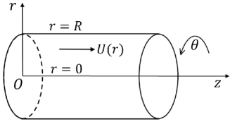
Figure 1: Schematic diagram showing the geometry and the coordinate system considered.

The rest of this paper is structured as follows: In Section 2, we outline the stability formulation for viscoelastic pipe Poiseuille flow subjected to infinitesimal amplitude axisymmetric disturbances; the base state and governing linearized differential equations are provided, followed by a brief description of the numerical schemes employed. In Section 3, we first recapitulate the key features of the Newtonian pipe flow spectrum, which is followed by a detailed discussion of the corresponding eigenspectra for an Oldroyd-B fluid, as $E$ is varied for fixed $\beta$ (Sec. 3.1), wherein the centre mode instability is first identified. The role of the continuous spectra (CS), in terms of their effect on the least stable/unstable modes belonging to the Newtonian P-branch, is discussed in Section 3.1.1. In Section 3.2, we present the viscoelastic eigenspectra for fixed $E$ and varying $\beta$, with the relation between the CS and the center mode being discussed in Sec. 3.2.1. The relative importance of the least stable/unstable centre modes vis-a-vis wall modes in viscoelastic pipe flow is highlighted in Section 3.3, where we also contrast the pipe flow scenario with the recent DNS results for viscoelastic channel flow (Shekar et al., 2019) which point to the crucial role of the critical layer corresponding to the least stable wall mode (the elastically modified Tollmien-Schlichting mode). Neutral stability curves are presented in Section 4, where the behaviour of the neutral curves for $k\ll 1$ obtained via a low-$k$ asymptotic analysis is shown to agree very well with those obtained from the full governing equations for $k\ll 1$. For sufficiently small $E$, there is a remarkable collapse of the neutral curves (Sec. 4.1) in the suitably rescaled $Re$–$k$ plane; a further collapse is obtained in the dual limit $E(1-\beta)\ll 1$ and $\beta\rightarrow 1$. In Section 4.2, we demonstrate how the critical parameters $\Rey_{c}$, $k_{c}$ and $c_{r,c}$ scale with $E$ in the limit $E\ll 1$, and justify the numerical results via scaling arguments in the limit of $Re\gg 1$, $E\ll 1$, when the unstable mode is confined in the neighbourhood of the centerline. In Sec. 4.3, we examine the role of stress diffusion in the constitutive relation to show that the unstable center mode persists for physically realistic values of the diffusion coefficient. Our theoretical predictions are compared (in a parameter-free manner) with the experimental observations of Samanta et al. (2013) and Chandra et al. (2018) in Section 4.4; herein, we also compare our predictions with the recent DNS results for viscoelastic pipe flow by Lopez et al. (2019). Finally, in Section 5, we summarize the salient findings of this study, and provide a discussion on how the discovery of a linear instability in viscoelastic pipe flow can play a pivotal role in clarifying the pathway to the MDR regime from the laminar state.

2 Problem formulation and numerical method

2.1 Governing Equations

We consider the linear stability of steady fully-developed flow of a viscoelastic fluid in a rigid circular pipe of radius $R$ as shown in Fig. 1. A cylindrical polar coordinate system is used with $r,\theta$ and $z$ denoting the radial, azimuthal and axial directions. The following scales are used for nondimensionalizing the governing equations: radius of the pipe $R$ for lengths, maximum base-flow velocity $U_{max}$ for velocities, $R/U_{max}$ for time and $\rho U_{max}^{2}$ for pressure and stresses, with $\rho$ being the density of the fluid.

The governing (nondimensional) continuity and Cauchy momentum equations are given by

$$\bnabla\bcdot\boldsymbol{v}=0,\quad\frac{\p\boldsymbol{v}}{\p t}+(\boldsymbol{v}\bcdot\bnabla)\boldsymbol{v}=-\bnabla p+\frac{\beta}{\Rey}\nabla^{2}\boldsymbol{v}+\bnabla\bcdot\mathsfbi{T}.$$

Here, $\boldsymbol{v}$ is the fluid velocity field, $p$ is the pressure field and $\mathsfbi{T}$ is the polymeric contribution to the stress tensor, which in turn is given by the Oldroyd-B constitutive relation (Larson, 1988) as follows

$$W\left(\frac{\p\mathsfbi{T}}{\p t}+\left(\boldsymbol{v}\bcdot\bnabla\right)\mathsfbi{T}-\mathsfbi{T}\bcdot\left(\bnabla\boldsymbol{v}\right)-\left(\bnabla\boldsymbol{v}\right)^{T}\bcdot\mathsfbi{T}\right)+\mathsfbi{T}=\frac{(1-\beta)}{\Rey}\{\bnabla\boldsymbol{v}+(\bnabla\boldsymbol{v})^{T}\}.$$ (2)

The solvent to solution viscosity ratio is denoted by $\beta=\eta_{s}/\eta$, where the solution viscosity is $\eta=\eta_{p}+\eta_{s}$, $\eta_{s}$ and $\eta_{p}$ being the solvent and polymer viscosities respectively; $\beta=0$ and $1$ denote the UCM and Newtonian limits. For a fixed $\beta$, the dimensionless groups relevant to the stability of the Oldroyd-B fluid above are the Reynolds number $\Rey=\rho U_{max}R/\eta$, the Weissenberg number $W=\lambda U_{max}/R$ which is a ratio of the polymer relaxation time $\lambda$ to the flow time scale. The Oldroyd-B model describes the stress in a dilute solution of polymer chains modelled as non-interacting Hookean dumbbells (Larson, 1988), and is invariably the first model used in the examination of elastic phenomena involving dilute polymer solutions. Consistent with the aforementioned microscopic picture, the Oldroyd-B model assumes the relaxation time to be independent of both the shear rate and the polymer concentration. Since the model predicts a shear-rate-independent viscosity, the non-Newtonian (elastic) effects in this model arise from an effective tension along the streamlines (arising from flow-aligned dumbbells), which manifests as a shear-rate-independent first normal stress different in viscometric flows. This model has been extensively used, and with considerable success, in earlier investigations of inertialess elastic instabilities in flows with curved streamlines (Larson et al., 1990; Shaqfeh, 1996; Pakdel & McKinley, 1996). The so-called Boger fluids constitute an experimental realization of this constitutive model (Boger & Nguyen, 1978). As discussed later in the manuscript (in Section 4.4.1, where we use scaling arguments in the context of the FENE-P model to assess the role of shear thinning), while shear-thinning can play an important role especially in flow through microtubes (Samanta et al., 2013; Chandra et al., 2018), the Oldroyd-B model does have the necessary ingredients to qualitatively predict the instabilities observed in experiments.

2.2 Base state

The base-state velocity profile is the classical Hagen-Poiseuille profile because the nonlinear terms in the upper-convected derivative of derivative of the polymer shear stress $T_{rz}$ are identically zero. The nondimensional base flow velocity vector is given by:

$$\overline{\boldsymbol{v}}=\left[\begin{array}[]{c}\bar{v}_{r}\\ 0\\ \bar{v}_{z}\\ \end{array}\right]=\left[\begin{array}[]{c}0\\ 0\\ U(r)\\ \end{array}\right],$$ (3)

where $U(r)=1-r^{2}$ for pipe Poiseuille flow. Here, and in what follows, base state quantities are denoted by an overbar. The polymer contribution to the stress tensor in the base state is given by

$$\overline{\mathsfbi{T}}=\left[\begin{array}[]{ccc}\bar{\tau}_{rr}&0&\bar{\tau}_{rz}\\ 0&\bar{\tau}_{\theta\theta}&0\\ \bar{\tau}_{zr}&0&\bar{\tau}_{zz}\\ \end{array}\right]=\frac{1}{\Rey}\left[\begin{array}[]{ccc}0&0&U^{\prime}\\ 0&0&0\\ U^{\prime}&0&2(1-\beta)WU^{\prime 2}\\ \end{array}\right],$$ (10)

where, $f^{\prime}\equiv\mathrm{D}f\equiv\frac{\mathrm{d}f}{\mathrm{d}r}$. Unlike the velocity profile, the base-state stress profile differs from that of a Newtonian fluid in having a tension along the streamlines proportional to the square of the velocity gradient.

2.3 Linear stability analysis

A temporal linear stability analysis is carried out wherein the base-state above is subjected to small amplitude axisymmetric perturbations. Because of the absence of a Squire-like theorem for pipe flow even in the simpler Newtonian case, in general, both axisymmetric and nonaxisymmetric disturbances need to be considered for viscoelastic Oldroyd-B fluids. However, for the parameter regime probed in this study, we find axisymmetric disturbances alone to be unstable, and this study is therefore restricted to axisymmetric disturbances. The total velocity, pressure and stress are expressed in terms of their base-state values and perturbations as v &= ¯v + ^v,
p = ¯p + ^p,
T = ¯T + ^T  , with $\hat{f}$ denoting the perturbation to the dynamical quantity $f$. For axisymmetric disturbances, the perturbation velocity and stress tensor are:

$$\hat{\boldsymbol{v}}=\left[\begin{array}[]{c}\hat{v}_{r}\\ 0\\ \hat{v}_{z}\\ \end{array}\right],\text{ and }\hat{\mathsfbi{T}}=\left[\begin{array}[]{ccc}\hat{\tau}_{rr}&0&\hat{\tau}_{rz}\\ 0&\hat{\tau}_{\theta\theta}&0\\ \hat{\tau}_{zr}&0&\hat{\tau}_{zz}\\ \end{array}\right].$$ (11)

Next, the perturbation quantities above are represented in the form of Fourier modes in the axial ($z$) direction in the following manner:

$$\hat{f}(r,z;t)=\tilde{f}(r)\mathrm{\exp}\{\mathrm{i}k(z-ct)\},$$ (12)

where $k$ is the axial wavenumber and $c=c_{r}+ic_{i}$ is the complex wave speed. The flow is temporally unstable (stable) if $c_{i}>0$ $(<0)$. Substituting Eq. 12 in the linearized versions of Eqs. $(1a,b)$–2, we obtain the following set of linearized governing equations:

$$\left(\mathrm{D}+\frac{1}{r}\right)\tilde{v}_{r}+\mathrm{i}k\tilde{v}_{z}=0,$$ (13)

$$G\tilde{v}_{r}=-\mathrm{D}\tilde{p}+\left[\left(\mathrm{D}+\frac{1}{r}\right)\tilde{\tau}_{rr}+\mathrm{i}k\tilde{\tau}_{rz}-\frac{\tilde{\tau}_{\theta\theta}}{r}\right]+\frac{\beta}{\Rey}\mathrm{L}\tilde{v}_{r},$$ (14)

$$G\tilde{v}_{z}+U^{\prime}\tilde{v}_{r}=-\mathrm{i}k\tilde{p}+\left[\left(\mathrm{D}+\frac{1}{r}\right)\tilde{\tau}_{rz}+\mathrm{i}k\tilde{\tau}_{zz}\right]+\frac{\beta}{\Rey}\left(\mathrm{L}+\frac{1}{r^{2}}\right)\tilde{v}_{z},$$ (15)

$$H\tilde{\tau}_{rr}=2\frac{(1-\beta)}{\Rey}\left(\mathrm{D}+W\mathrm{i}kU^{\prime}\right)\tilde{v}_{r},$$ (16)

$$H\tilde{\tau}_{rz}-WU^{\prime}\tilde{\tau}_{rr}=\frac{(1-\beta)}{\Rey}[\{\mathrm{i}k-W\left(U^{\prime\prime}-U^{\prime}\mathrm{D}-2\mathrm{i}kWU^{\prime 2}\right)\}\tilde{v}_{r}$$

$$+\left(\mathrm{D}+W\mathrm{i}kU^{\prime}\right)\tilde{v}_{z}],$$ (17)

$$H\tilde{\tau}_{\theta\theta}=2\frac{(1-\beta)}{\Rey}\frac{\tilde{v}_{r}}{r},$$ (18)

$$H\tilde{\tau}_{zz}-2WU^{\prime}\tilde{\tau}_{rz}=2\frac{(1-\beta)}{\Rey}[-2W^{2}U^{\prime}U^{\prime\prime}\tilde{v}_{r}+\{\mathrm{i}k+WU^{\prime}\left(\mathrm{D}+2W\mathrm{i}kU^{\prime}\right)\}\tilde{v}_{z}],\newline$$ (19)

where $G=\mathrm{i}k(U-c)$, $H=1+WG$ and $\mathrm{L}=\left(\mathrm{D}^{2}+\frac{\mathrm{D}}{r}-\frac{1}{r^{2}}-k^{2}\right)$. The no-slip boundary conditions $\tilde{v}_{r}=0$ and $\tilde{v}_{z}=0$ are applicable at $r=1$, while at $r=0$, the conditions $\tilde{v}_{r}=0$ and $\tilde{v}_{z}=\text{finite}$, corresponding to regularity of axisymmetric disturbances in the vicinity of the centerline, are used (Batchelor & Gill, 1962; Khorrami et al., 1989).

2.4 Numerical method

We use two independent formulations to solve the viscoelastic eigenvalue problem for the wavespeed $c$. In the first, the governing equations for perturbation stresses (Eqs. 16–19) are substituted in Eqs. 14–15 to obtain two linearized ordinary differential equations corresponding to the momentum balances in $r$- and $z$-directions in addition to Eq. 13, and the dependent variables in this formulation are $\tilde{v}_{r}$, $\tilde{v}_{z}$ and $\tilde{p}$. In the second formulation, we directly solve the system of linear equations (Eqs. 13–19), with $\tilde{v}_{r}/r$ as the dependent variable instead of $\tilde{v}_{r}$, with the other variables being $\tilde{v}_{z}$, $\tilde{p}$, $\tilde{\tau}_{\theta\theta}$, $\tilde{\tau}_{rr}$, $\tilde{\tau}_{rz}$, and $\tilde{\tau}_{zz}$. The simplified equations represent a homogeneous eigenvalue problem, and are solved using the standard spectral collocation numerical scheme based on Chebyshev polynomials (Boyd, 2000; Trefethen, 2000). Results from the two different spectral approaches show excellent agreement. Further, the eigenvalues obtained from the spectral method were verified using a shooting method (Ho & Denn, 1977; Lee & Finlayson, 1986) implemented for the first formulation, based on an adaptive step size Runge-Kutta integrator and a Newton-Raphson procedure for determining the eigenvalue. The integration for the shooting method was carried out from a point near the centerline $r=\epsilon$ (with $\epsilon\rightarrow 0$) to the pipe wall at $r=1$. The velocities at $r=\epsilon$ were obtained using a Frobenius series expansion (Garg & Rouleau, 1972) about the regular singular point $r=0$. The shooting method gives very accurate (based on our choice of tolerance, typically $10^{-9}$) results when sufficiently close initial guesses are provided, whereas the number of polynomials $N$ required for convergence of eigenvalues in the spectral method depends mainly on the nature of the eigensolutions and the parameter values. Typically, the $N$ required for convergence of eigenvalues for finite $\beta$ is in the range $150$–$200$, while that for the UCM limit ($\beta\rightarrow 0$), is in the range $400$–$500$. There is no prior literature which reports the eigenspectrum for pipe flow of an Oldroyd-B fluid, and hence our numerical procedure was benchmarked in the Newtonian limit (obtained by setting $W=0$ or $\beta=1$). Results in this limit are available, for instance, in Schmid & Henningson (1994, 2001).

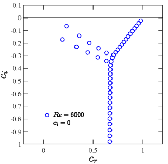
(a) $Re=6000$

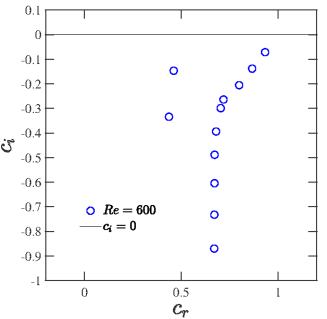
(b) $Re=600$

Figure 2: The ‘Y’-shaped eigenspectrum for Newtonian pipe flow subjected to axisymmetric disturbances for $k=3$, and for $Re=6000$ and $600$.

3 General features of the viscoelastic pipe flow eigenspectrum

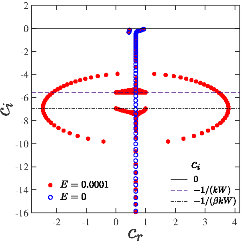
(a) $E=10^{-4}$

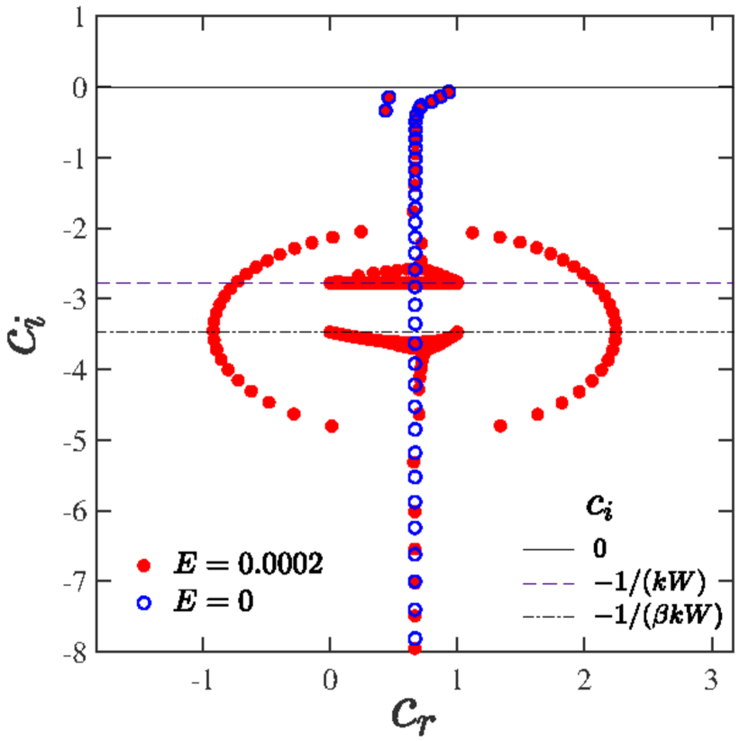
(b) $E=2\times 10^{-4}$

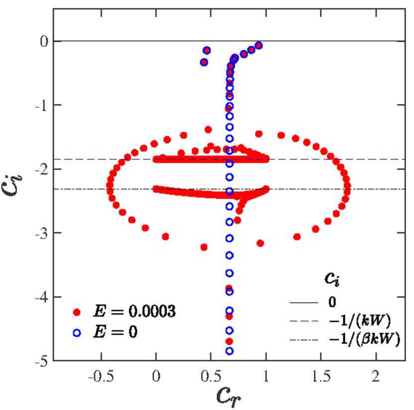
(c) $E=3\times 10^{-4}$

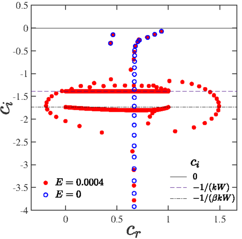
(d) $E=4\times 10^{-4}$

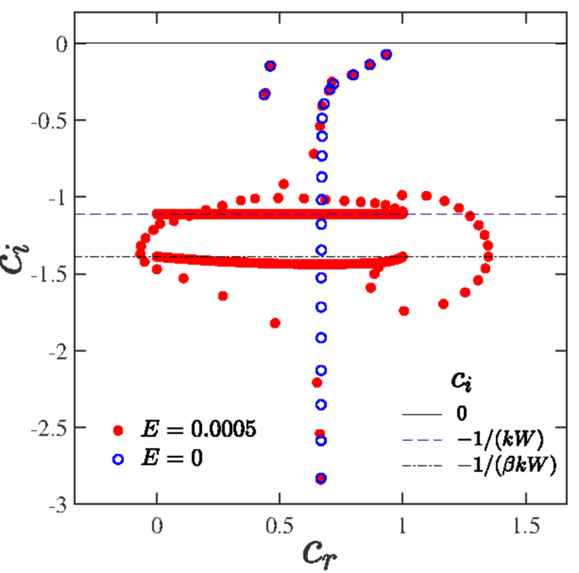
(e) $E=5\times 10^{-4}$

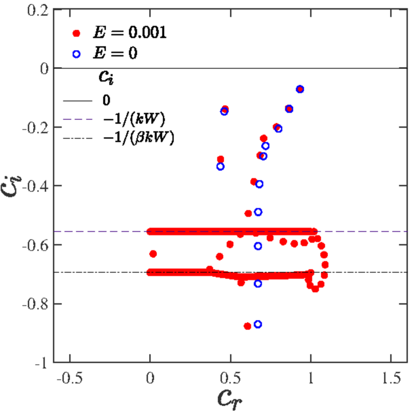
(f) $E=10^{-3}$

Figure 3: Eigenspectra for pipe flow of an Oldroyd-B fluid at $\beta=0.8,\Rey=600$ and $k=3$, and for different $E$ in the range $5\times 10^{-4}$–$10^{-3}$. The eigenspectra are obtained for $N=200$, and there is excellent convergence of the spectra for $N=200$ and $250$ (not shown). An elliptical-ring structure is prominent at the lower $E$’s, but is absent beyond $E=10^{-3}$. The vertical locations of the CS1 and CS2 lines and the Newtonian spectrum for the same $\Rey$ and $k$ are shown for reference.

We first discuss results obtained for pipe Poiseuille flow of Oldroyd-B fluids, with the extensive aid of eigenspectra, and demonstrate how the viscoelastic spectrum differs substantially from its Newtonian counterpart. Sections 3.1 and 3.2, respectively, consider the variation in the eigenspectrum with increasing $E$ (from zero) at a fixed $\beta$, and with variation in $\beta$ at a fixed $E$. The focus is on the locations of the least stable modes, and as to how they change with changing $E$ and $\beta$. Alongside, we also demonstrate (Secs. 3.1.1 and 3.2.1) how the continuous spectra (henceforth abbreviated as ‘CS’) play an important role in the emergence of the eigenmode (a center mode) that eventually becomes unstable. In Sec. 3.3, we contrast the nature of the least stable modes in viscoelastic pipe and channel flows, showing, in particular, that for the parameters corresponding to viscoelastic channel flow where the wall (TS) mode is least stable (Shekar et al., 2019), pipe flow has the center mode as its least stable mode. The center mode instability is characterized further using neutral stability curves in the $Re$-$k$ plane at fixed $E$ and $\beta$ (Sec. 4), which are shown to collapse when plotted using suitable rescaled variables (Sec. 4.1). The variation of the minima of the $Re$-$k$ neutral curves (the critical Reynolds number $Re_{c}$) and the corresponding critical wavenumber $k_{c}$ is explored (Sec. 4.2) for different $E$ and $\beta$, and scaling relationships are obtained in the limit $E\ll 1$ and $E\ll 1$, $(1-\beta)\ll 1$. It is then shown that the scaling results inferred from the numerics are consistent with those obtained from a boundary-layer analysis near the pipe centerline. We finally compare our theoretical predictions with recent experimental and DNS studies in Sec. 4.4.

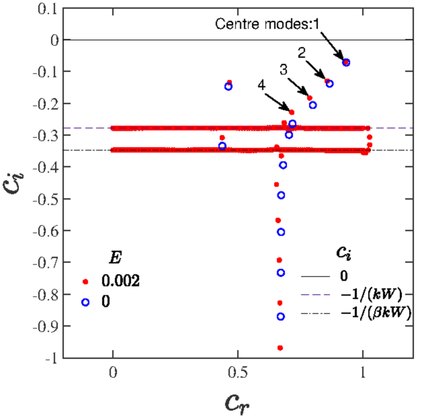
(a) $E=0.002$

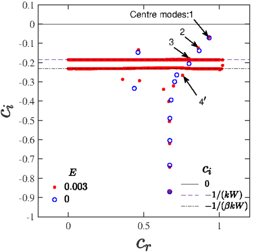
(b) $E=0.003$

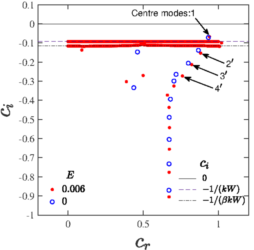
(c) $E=0.006$

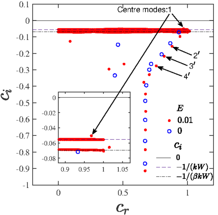
(d) $E=0.01$

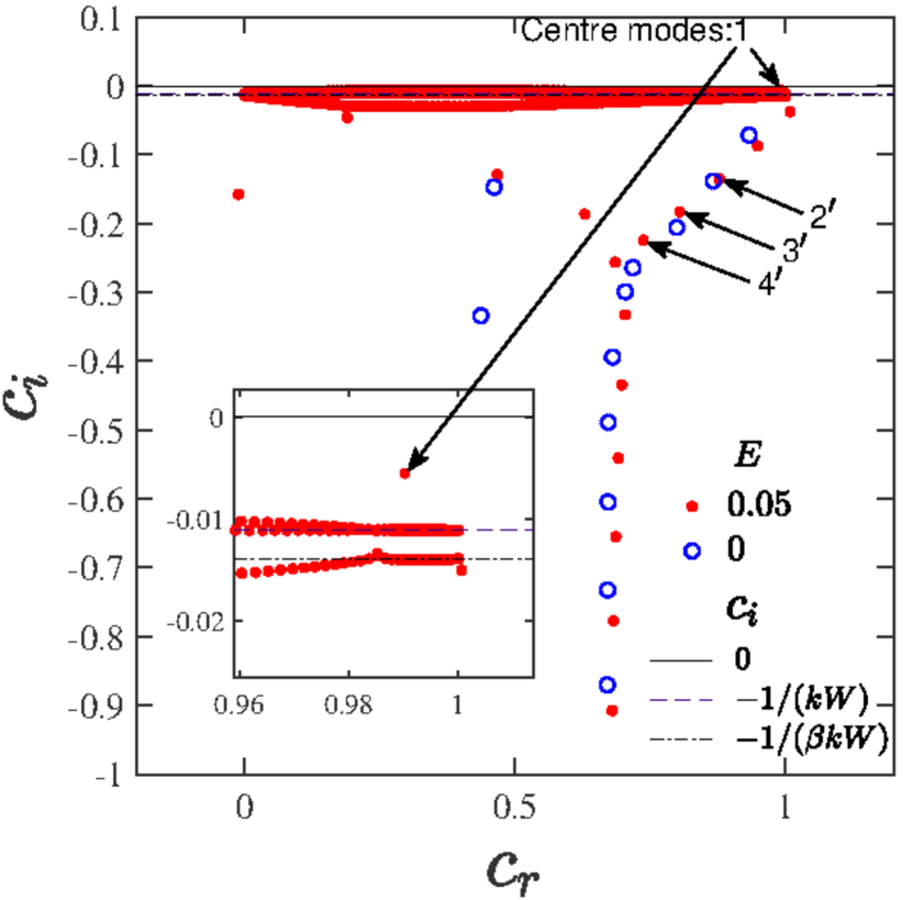
(e) $E=0.05$

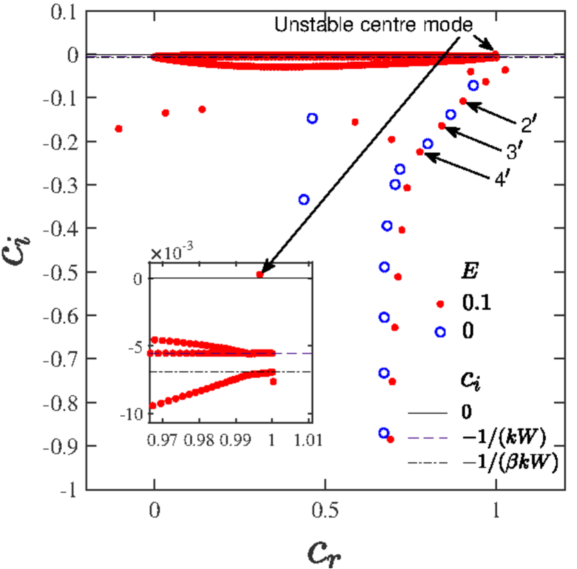
(f) $E=0.1$

Figure 4: Eigenspectra for the Oldroyd-B fluid for different $E$ in the range $0.002$–$0.1$, at $\beta=0.8$, $\Rey=600$, $N=200$, and $k=3$. The spectra, shown for a narrower range of $c_{r}$ and $c_{i}$ compared to Fig. 3, demonstrate how the discrete center modes (labelled $2$, $3$, and $4$) merge into and emerge out (labelled $2^{\prime}$, $3^{\prime}$, and $4^{\prime}$) of the CS as $E$ is increased. The least stable center mode (labelled 1) always stays above the CS, and eventually becomes unstable at $E=0.1$. The vertical locations of the CS lines and the Newtonian spectrum at the same $\Rey$ and $k$ are shown for reference.

3.1 Spectra at fixed $\beta$ and different $E$

Figures 2(a) and 2(b) show the eigenspectra for Newtonian pipe flow at $Re=6000$ and $Re=600$ respectively. The spectrum has the well-known ‘Y’-shaped structure (Schmid & Henningson, 2001; Mack, 1976) at $Re=6000$, but this is only beginning to form in the spectrum at $Re=600$. The Y-shaped structure is comprised of three branches: (i) the ‘A branch’ corresponding to ‘wall modes’ with $c_{r}\rightarrow 0$ for $\Rey\gg 1$ on the top left; (ii) the ‘P branch’ which consists ‘center modes’ with $c_{r}\rightarrow 1$ for $\Rey\gg 1$ on the top right, and (iii) the ‘S branch’ which consists modes with $c_{r}\approx 2/3$ extending down to $c_{i}=-\infty$. For $Re\gg 1$, the decay rates of the least stable center and wall modes vary as $|c_{i}|\sim Re^{-1/2}$ and $|c_{i}|\sim Re^{-1/3}$ respectively (Meseguer & Trefethen, 2003), implying that the center modes are the least stable at large $\Rey$. Although these scalings need not necessarily hold for the moderate $Re$ ($=600$) considered in Figs. 3 and 4 below, the center mode is nevertheless found to be the least stable one. Consistent with previous studies (Schmid & Henningson, 1994, 2001), all modes for Newtonian pipe flow are found to be stable. We discuss the nature of the least stable mode in more detail below in Sec. 3.3.

The spectra for pipe flow of an Oldroyd-B fluid reduce to the Newtonian one either when $E\rightarrow 0$ (at fixed $\beta$) or when $\beta\rightarrow 1$ (at fixed $E$). We therefore first examine the effect of viscoelasticity as $E$ is increased from zero, with $\beta$ fixed at $0.8$. Figures 3 and 4 show the viscoelastic eigenspectra for $Re=600$, with $E$ ranging from $5\times 10^{-4}$ to $0.1$. The values of $\beta$ and $Re$ are chosen so they are close to the experimental conditions of Samanta et al. (2013) and our earlier theoretical work (Garg et al., 2018). With increasing $E$, Figs. 3 and 4 show the classical Y-shaped structure of the Newtonian spectrum to be altered by elasticity in a singular manner. There are important differences between the two spectra even for the smallest $E$’s, the most prominent of these being the appearance of two continuous spectra for the viscoelastic case, similar to viscoelastic plane shear flows (Renardy & Renardy, 1986; Sureshkumar & Beris, 1995; Graham, 1998; Wilson et al., 1999; Grillet et al., 2002; Chokshi & Kumaran, 2009). It is now well understood (Graham, 1998; Chaudhary et al., 2019; Subramanian et al., 2020) that the continuous spectra arise from the local nature of the constitutive model for the polymeric stress, and disappear when non-local diffusive effects are incorporated in the constitutive relation (see Sec. 4.3). The eigenvalues corresponding to the CS are obtained by setting to zero the coefficient of the highest order derivative in the differential equation governing the stability. This coefficient turns out to be the product $[1+\mathrm{i}kW(U-c)][1+\beta\mathrm{i}kW(U-c)]$, which leads to a pair of horizontal ‘lines’ in the $c_{r}$–$c_{i}$ plane with $c_{i}=-1/(kW)$ and $c_{i}=-1/(\beta kW)$, and with $0\leq c_{r}\leq 1$. Henceforth, these two continuous spectra are respectively abbreviated as ‘CS1’ and ‘CS2’ respectively, with CS1 being present even in the limit of a UCM fluid, and CS2 being present only when there is a solvent contribution ($\beta\neq 0$), receding to $c_{i}=-\infty$ in the limit $\beta\rightarrow 0$.

Figure 3 explores the spectra for the smallest $E$’s (ranging from $10^{-4}$ to $10^{-3}$), the range of $c_{r}$ and $c_{i}$ being chosen so as to provide a larger view of the spectra. Here, in addition to the modified Y-shaped structure of the Newtonian spectra and the two CS lines, there exist a class of modes which form a ‘ring’ that surrounds the continuous spectra at small $E$’s of $O(\sim 10^{-4})$. Similar to CS1 and CS2 , all modes belonging to the ring structure are stable for the range of $E$ explored. For small $E$’s, the modes on the ring appear to be symmetrically distributed (Figs. 3(a) to 3(c)) about the S branch, forming an approximate ellipse. As $E$ is increased, the modes move towards the continuous spectra with the ring getting smaller in size. For $E=4\times 10^{-4}$, these modes move closer, intermingling with the other modes which emerge from the CS (Fig. 3(d)), and the ring structure is now fully distorted. At still higher $E\sim 10^{-3}$ (see Figs. 3(e) and 3(f)), the modes originally on the ring collapse, wrapping around the CS in an irregular manner. To understand the origin of the ring structure, it is relevant to recall a prominent feature of the viscoelastic spectra (at nonzero $Re$) in the UCM limit ($\beta=0$): an infinite sequence of discrete modes corresponding to damped shear waves in a viscoelastic fluid (discussed below in Sec. 3.2), and are referred to as the high-frequency-Gorodtsov-Leonov (‘HFGL’) modes (Gorodtsov & Leonov, 1967; Kumar & Shankar, 2005; Chaudhary et al., 2019). This sequence corresponds to $c_{i}=-1/(2kW)$, and extends to infinity in either direction parallel to the $c_{r}$ axis. As we demonstrate below in Fig. 10, at any finite $\beta$, the infinite-in-extent HFGL line curves downwards, eventually meeting the S branch, and thereby leading to the aforementioned ring structure for sufficiently small $E$.

In Fig. 4, we explore the spectra for larger $E$, in the range $0.002$–$0.1$, with the ranges of $c_{r}$ and $c_{i}$ being chosen to provide a more magnified view of the spectra. As $E$ is increased, the vertical locations of the two CS move up towards $c_{i}=0$, and in the process, the discrete ‘elastic’ center modes (labelled 2, 3, 4 in Fig. 4(a); and that lie above the CS) disappear into the CS. As $E$ is increased further, new discrete elastic center modes (now shown with the labels $2^{\prime}$, $3^{\prime}$, and $4^{\prime}$ in Figs. 4(c) and 4(d), which lie below the CS) emerge out of the CS. The labelling of the modes that emerge below the CS are for the purposes of reference only, and there is no connection between these modes (with primes) and the ones (without primes) that disappeared into the CS. This was ascertained from the absence of any resemblance between the eigenfunctions of the modes that disappear into and reappear from the CS. A more detailed account of the evolution of the center modes as $E$ is varied is provided below in Fig. 7. Importantly, the least stable center mode (labelled 1) does not merge into the CS, and always stays above it. As $E$ is increased to $0.1$, this center mode becomes unstable, and corresponds to the instability first reported in Garg et al. (2018). This scenario of the unstable center mode being a smooth continuation of its stable Newtonian counterpart is, however, sensitive to $\beta$, and we show below (and in more detail in Sec. 3.1.1) that there exist other parameter regimes where the center mode that eventually becomes unstable emerges out the CS with increasing $E$, and there is no connection to the least stable Newtonian center mode. Other new stable center modes (with $c_{r}\rightarrow 1$; see Figs. 4(d)–4(f)) and wall modes (with $c_{r}\rightarrow 0$, and even negative; see Figs. 4(e) and 4(f)), which have no Newtonian counterparts, appear below the CS with increasing $E$. Increase in $E$ has a stabilizing effect on these modes. The aforementioned annihilation and creation of discrete modes with increase in $E$ occurs because both the continuous spectra are branch cuts (Wilson et al., 1999) for Poiseuille flow. Note that, for plane Couette flow, only CS2 is a branch cut. It is well known that discrete eigenmodes can appear or disappear out of the branch cut as parameters are varied, and this aspect is discussed further in Sec. 3.1.1 in the specific context of the center mode.

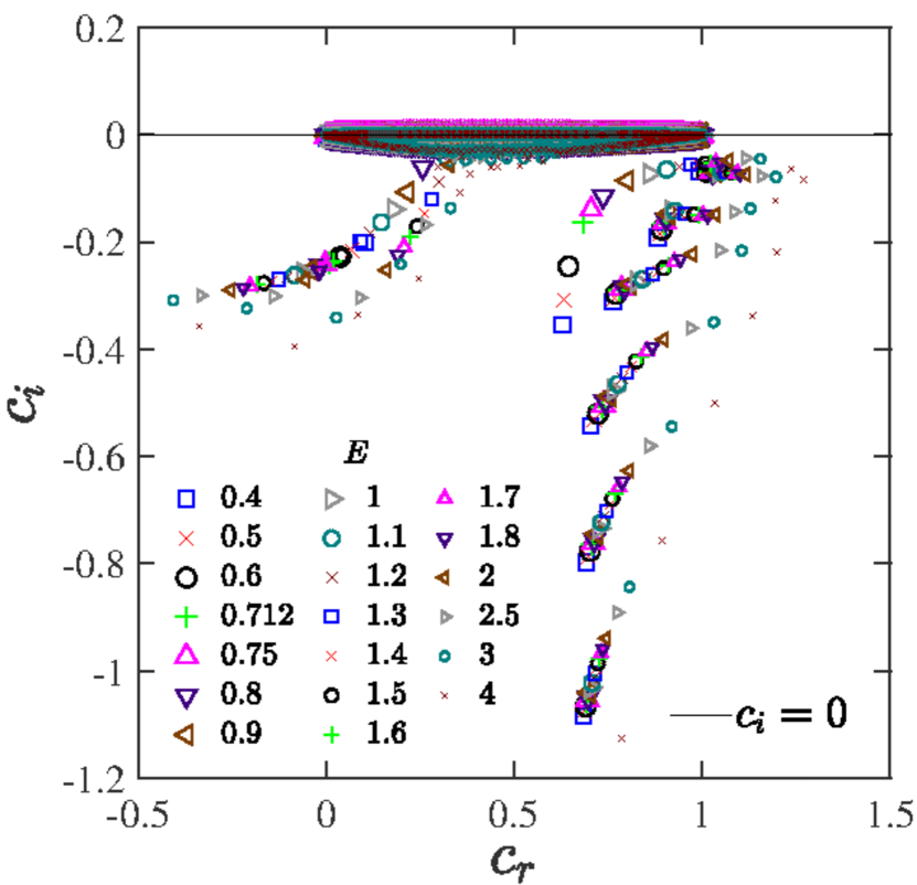
(a) Unfiltered spectra

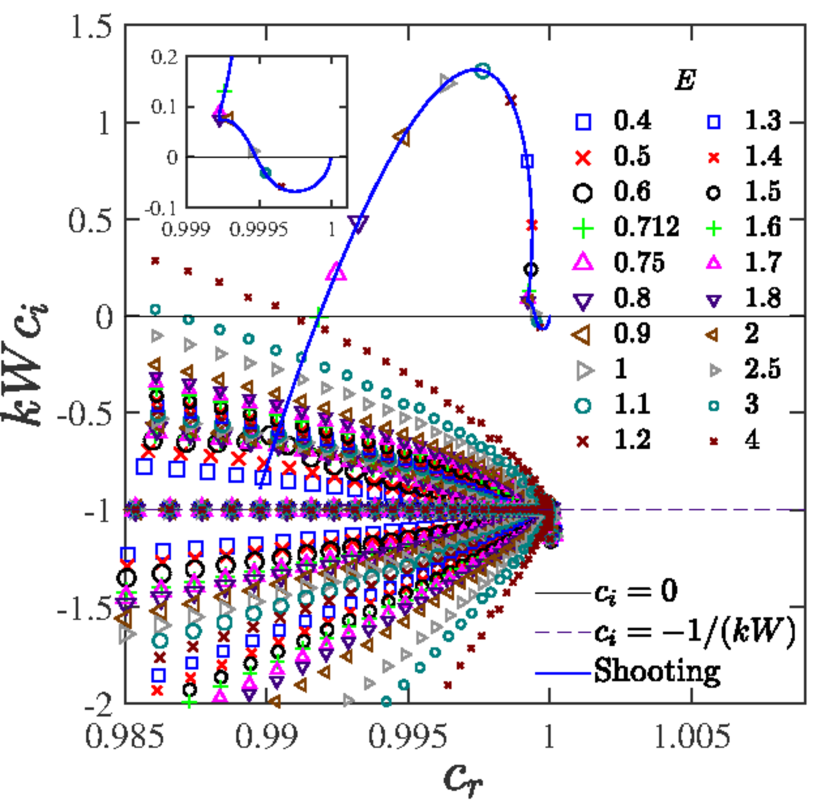
(b) Magnified region near $c_{r}=1$

Figure 5: (a) Eigenspectra for different values of $E$ for $\beta=0.96,\Rey=500,k=1$; (b) Enlarged version of region in panel (a) near the unstable center mode. The scaled growth rate $kWc_{i}$ fixes the vertical location of both the CS (for $\beta=0.96$, CS1 and CS2 lie very close to each other). The continuous line for the trajectory of the unstable center mode is obtained using the shooting method.

Figure 5 shows the spectra in the near-Newtonian limit of $\beta=0.96$ and for $E$ ranging over the interval $(0.4,4)$, overlaid in a single plot, in order to demonstrate the variation of not just the (eventually) unstable center mode, but also of the other stable modes. For the higher $E$’s considered in Fig. 5, the two CS’s lie very close to $c_{i}=0$ (and to each other for the chosen $\beta$), and the modes in the Newtonian P-branch have therefore already disappeared into the CS, with new modes emerging from below. Thus, the trajectories of the modes shown in Fig. 5(a) are for the modes that start off below the CS. The zoomed version in Fig. 5(b) shows the spectra in terms of the scaled growth rate $kWc_{i}$, which fixes the vertical location of both the CS (for fixed $\beta$), and allows one to focus on the trajectory of the unstable center mode with varying $E$. The continuous curve indicating the trajectory of the center mode, as $E$ is varied, is obtained using the shooting method with much finer increments in $E$. This figure shows that the center mode first emerges out of the CS, in the form of a bump in the continuous spectrum balloon, at $E\approx 0.6$, and becomes unstable as $E$ is increased to $0.712$. The center mode remains unstable for $0.712\leq E\leq 2.5$, but becomes stable for $E>2.5$, with $|c_{i}|$ eventually scaling as $1/E$ for large $E$. Thus, Figs. 4 and 5(b) show that there are two qualitatively different trajectories of the unstable center mode with increasing $E$. For the lower $\beta$ $(=0.8)$, the center mode appears as a smooth continuation of the least stable Newtonian center mode, while for $\beta=0.96$, it emerges from the continuous spectrum, with no obvious connection to the Newtonian spectrum. This aspect is discussed in more detail below in Sec. 3.1.1.

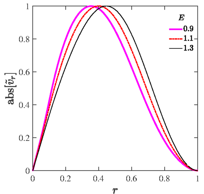
(a) Radial velocity

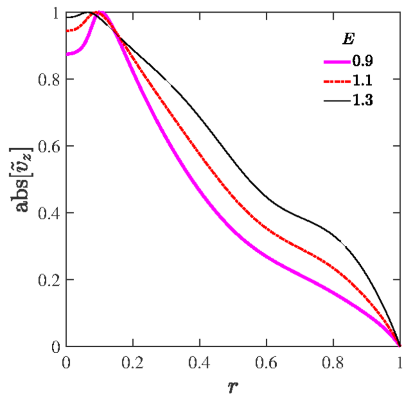
(b) Axial velocity

(c) $rz$ polymer stress

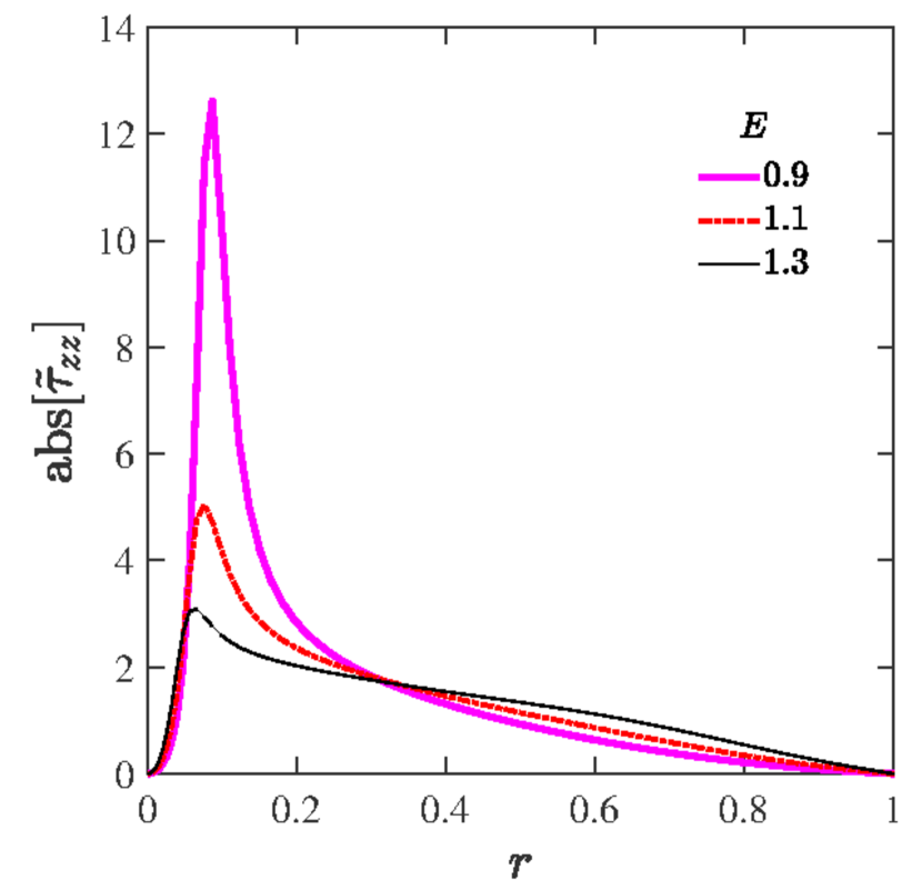
(d) $zz$ polymer stress

Figure 6: Velocity and polymer stress eigenfunctions corresponding to the unstable centre modes (in Fig. 5(b)) at different $E$ for $\beta=0.96,\Rey=500$ and $k=1$.

Figures 6(a)–6(d) show the velocity ($v_{r}$ and $v_{z})$ and stress ($T_{rz}$ and $T_{zz}$) eigenfunctions, for different $E$, corresponding to few of the unstable center modes shown in Fig. 5(b). The velocity and $T_{rz}$ eigenfunctions are largely insensitive to variations in $E$, but the $T_{zz}$ eigenfunction shows a distinct and sharp peak for the smaller $E$ ($=0.9$) near the radial location where the phase speed of the disturbances equals the local base flow velocity. While the amplitudes of the axial velocity eigenfunctions in Fig. 6 are larger near the central core region of the pipe, the disturbance fields are nevertheless spread across the entire pipe cross-section for the parameters considered. As shown below (Section 4.2), only for sufficiently large $Re$ ($>1000$) does the localization of the velocity eigenfunctions near the center become prominent. It is worth emphasizing this feature here because recent studies (Shekar et al., 2019) have inaccurately characterized the center mode instability, analyzed in Garg et al. (2018) and the present work, as always being localized in the vicinity of the centerline regardless of $\Rey$.

3.1.1 The origin of the center mode at fixed $\beta$ and varying $E$

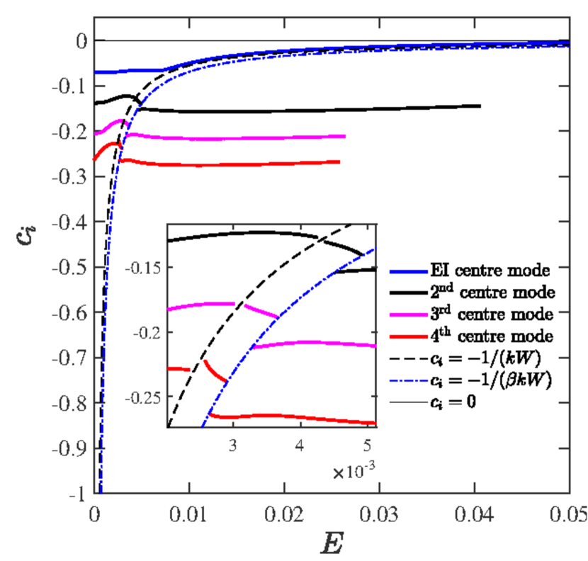
(a) Growth rates

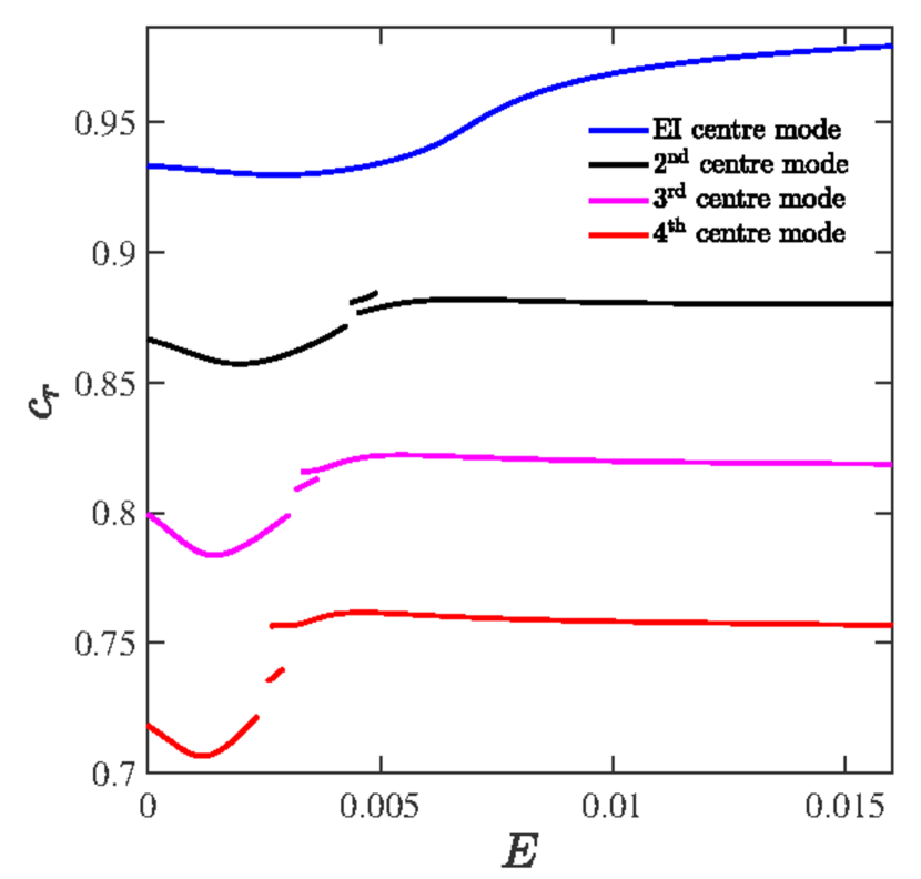
(b) Phase speeds

Figure 7: Effect of increasing $E$ on the first four least-stable center modes of Newtonian origin for $\beta=0.8,\Rey=600$ and $k=3$. (a) Growth rate vs. $E$, with the inset presenting the magnified view of the jumps suffered by the individual modes as they cross CS1 ($c_{i}=-1/(kW)$) and CS2 ($c_{i}=-1/(\beta kW)$). (b) Phase speeds corresponding to the modes shown in panel (a).

The origin of the center mode is more clearly demonstrated in Fig. 7(a) through the variation of $c_{i}$ with $E$ for the first four least-stable modes from the Newtonian P-branch, obtained using the shooting method. For $\beta=0.8$, consistent with the spectra in Fig. 4, the least stable Newtonian center mode always lies above the CS (Fig. 7(a)), smoothly continuing with increasing $E$, eventually becoming unstable for $E\approx 0.1$ (shown later in inset (A) of Fig. 9(a)). However, the other (more) stable Newtonian center modes (labelled $2$,$3$,$4$ in Fig. 4(a)) vanish into CS1 as $E$ is increased, and new modes appear out of CS1 with further increase in $E$, subsequently suffering a second jump across the CS2 line. The modes that emerge out of CS2 were the ones identified as and $2^{\prime}$,$3^{\prime}$ and $4^{\prime}$ in the spectra in Fig. 4. This feature is also evident in the variation of the phase speeds with $E$ in Fig. 7(b). An analogous phenomenon was reported by Chokshi & Kumaran (2009) for the least stable wall mode in plane Couette flow of an Oldroyd-B fluid.

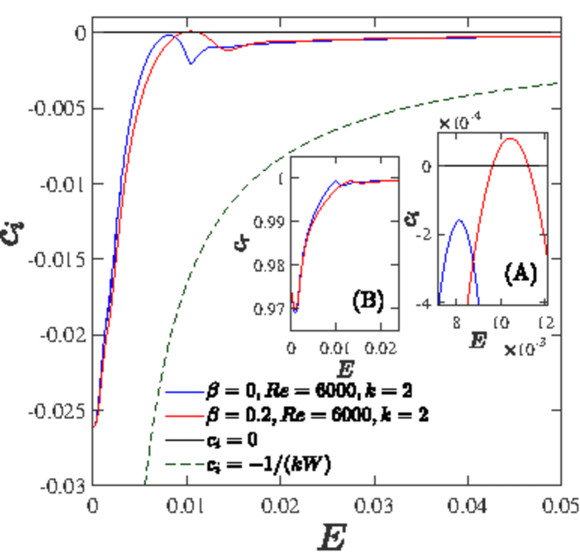
(a) $\beta=0$ and $0.2$

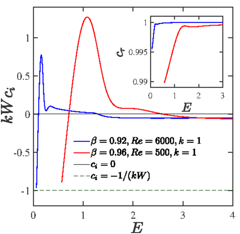
(b) Scaled growth rate for $\beta=0.92$ and $0.96$

Figure 8: Effect of increasing $E$ on the least stable Newtonian center mode for UCM and Oldroyd-B fluids: (a) $c_{i}$ for the least stable center mode at $Re=6000$ for $\beta=0$ and $0.2$, and the inset (A) shows the enlarged region near unstable range of the mode. Inset (B) shows the corresponding phase speeds. (b) Scaled growth rate of elasto-inertial modes at $Re=6000$, $\beta=0.92$ and $Re=500$, $\beta=0.96$, and the inset shows the corresponding phase speeds.

In Fig. 8(a), we examine the effect of increasing $E$ in the UCM and near-UCM limits at fixed $\Rey$ and $k$ (note that, regardless of the value of $\beta$, $E=0$ corresponds to the Newtonian limit). For $\beta=0$, the decay rate of the least stable Newtonian center mode decreases with increasing $E$, even to the point of reducing to $\sim 2\times 10^{-4}$ at $E\approx 8\times 10^{-3}$ (about 1/100^th of the decay rate in the Newtonian limit), but the mode remains stable. Since elastic effects are responsible for the unstable center mode, it might be expected that this instability should persist even in the absence of solvent contribution to the stress. The eigenspectra for pipe flow of a UCM fluid were computed for a vast range of parameters $0.5<k<3$, $100<Re<20000$, and $0<E<1$. Unlike the spectrum for plane channel flow of a UCM fluid (Sureshkumar & Beris, 1995; Chaudhary et al., 2019), only stable modes were obtained for pipe flow of a UCM fluid subjected to axisymmetric disturbances. Thus, as originally stated in Garg et al. (2018), the center mode instability in viscoelastic pipe flow requires the combined effects of both the polymer elasticity and solvent viscous effects, in addition to fluid inertia.

For $\beta=0.2$ (see Fig. 8(a)), however, the least stable Newtonian center mode does become unstable for $0.01<E<0.011$. For both $\beta$’s, the center mode trajectory is similar to that shown in Fig. 7, in that it remains above the CS over the range of $E$ examined. The corresponding phase speeds (inset (B) of Fig. 8(a)), for both $\beta=0$ and $\beta=0.2$, show a weak non-monotonic behaviour with $E$, although $c_{r}\leq 1$ for all $E$. The contrasting behaviour for $\beta$ close to unity (representing dilute solutions) is shown in Fig. 8(b). The main figure shows the variation of the scaled growth rate $kWc_{i}$ with $E$ for two different sets of (near-unity) $\beta$ and $Re$. The instability occurs at significantly larger values of $E\sim O(1)$, in contrast to Fig. 8(a), and the unstable range of $E$’s is also larger. In contrast to the trend for $\beta=0.2$, the continuation of the Newtonian center modes for both $\beta=0.92$ and $0.96$ collapses into the CS at smaller $E$’s (not shown). It is the trajectories of the new discrete modes, that emerge from the CS at slightly larger $E$’s, and that become unstable for $E\sim O(1)$, that are shown in Fig. 8(b). The corresponding phase speeds for $\beta=0.92$ and $0.96$ are shown in the inset of Fig. 8(b).

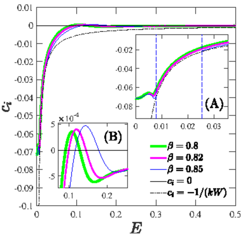
(a) Growth rates

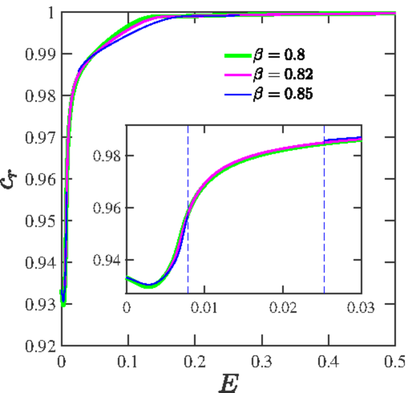
(b) Phase speeds

Figure 9: Effect of increasing $E$ on the viscoelastic centre mode for fixed values of $\beta=0.8,0.82$ and $0.85,\Rey=600$ and $k=3$: (a) Growth rates, with inset (A) showing the enlarged region over the range of $E$ for which the centre mode is discontinuous (marked by vertical dotted lines) due to CS1 with $c_{i}=-1/(kW)$. The locations of CS2 (with $c_{i}=-1/(\beta kW)$) are not shown owing to the closely-separated values of $\beta$ used in this figure. Inset (B) shows the region where the centre mode is unstable for all the three values of $\beta=0.8,0.82$ and $0.85$. (b) Phase speeds corresponding to the modes shown in panel (a). Inset in panel (b) shows the enlarged region near $E\rightarrow 0$.

In Figs. 7 and 8, we have seen two different trajectories for the center mode, as a function of $E$, depending on $\beta$. In order to clarify the change in the nature of the center mode trajectory - from a continuous variation of $c_{i}$ with increasing $E$ at smaller $\beta$, to a discontinuous variation for near-unity $\beta$ - Fig. 9(a) shows the behaviour of the center mode for $\beta=0.8$, $0.82$ and $0.85$. The center mode trajectory remains above CS1 until instability, for both $\beta=0.8$ and $0.82$, while for $\beta=0.85$, the center mode disappears into the CS at $E\approx 0.009$ (inset (A) of Fig. 9(a)). Thus, in this case, there exists a range $0.009\lessapprox E\lessapprox 0.024$ where the center mode does not exist. This range, which extends from the point of encounter of this mode with CS1 to the point of emergence of the new mode from CS1 at higher $E$, varies with increasing $\beta$. Evidently, the critical $\beta$, below which the center mode is a smooth continuation of the least stable Newtonian center mode, lies somewhere between $0.82$ and $0.85$ (for $Re=600$ and $k=3$). Note that, despite the discontinuous transition in terms of the collapse into the CS’s, the interval of instability in $E$ varies smoothly with increasing $\beta$ (the inset (B) in Fig. 9(a)). Figure 9(b) shows the corresponding phase speeds, and the enlarged region in the inset shows that the trend for $c_{r}$ vs $E$ curves is more or less same for $\beta=0.8,0.82$ and $0.85$, except for $\beta=0.85$, where the absence of the mode in the interval $0.009\lessapprox E\lessapprox 0.024$ leads to a gap in the $c_{r}$ curve.

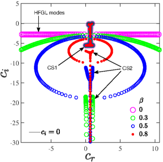
Figure 10: Eigenspectra for $E=10^{-4}$, $Re=600$, and $k=3$ demonstrating the bending down of the HFGL modes with increasing $\beta$, leading to the appearance of a ring-like structure for the higher $\beta$’s. The vertical location of CS1 is independent of $\beta$, while that of CS2 varies with $\beta$.

3.2 Spectra at fixed $E$ and different $\beta$

We next examine the viscoelastic eigenspectra as $\beta$ is increased from zero, at fixed $E$. We begin with Fig. 10 which illustrates the effect of increasing $\beta$, starting from the UCM spectrum, at $E=10^{-4}$. A moderate $Re$ ($=600$) is chosen in order to keep the spectral features relatively simple, requiring only a modest resolution (the number of collocation points $N$), and thereby allowing us to focus on the large-scale features. Figure 10 illustrates the singular feature of the bending down of the HFGL line for non-zero $\beta$. The bending down can be interpreted as a (very strong) stabilization of these modes due to the solvent viscosity. For the larger $\beta$’s ($\beta=0.5$ and $0.8$), the bending is ‘complete’, leading to the ring-like structure within the range of $c_{i}$’s examined; this then clarifies the origin of the structure seen before in Fig. 3. Figure 11 shows spectra at a higher $Re$ ($=6000$), for different $\beta$, and with $E=0.01$. The spectrum for $\beta=0$ (Fig. 11(a)) now has a more intricate structure, necessitating a zoomed view into the phase speed interval $(0,1)$. The features of the high-$Re$ UCM channel-flow spectrum were first explained in Chaudhary et al. (2019), and include CS1 (which appears as a balloon owing to the finite resolution), the HFGL, and additional discrete modes with $c_{r}\in[0,1]$ which lie on either side of the HFGL line , rougly along the contours of an ‘hourglass’. These features of the UCM pipe-flow spectrum, in Fig. 11(a), are analogous to the channel flow case above.

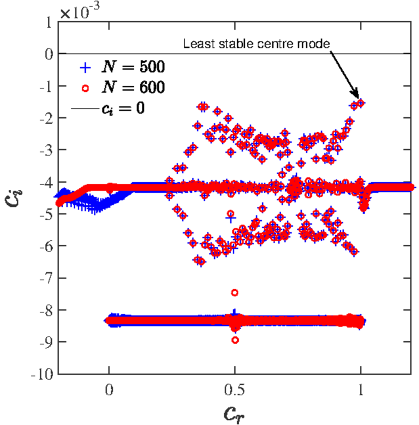
(a) $\beta=0$, UCM

(b) $\beta=1\times 10^{-4}$

(c) $\beta=5\times 10^{-4}$

(d) $\beta=5\times 10^{-3}$

(e) $\beta=5\times 10^{-2}$

(f) $\beta=0.2$

Figure 11: Unfiltered viscoelastic eigenspectra for $E=0.01,\Rey=6000$, $k=2$ and different $\beta$. The decay rate of the least stable centre mode in the UCM limit decreases with increase in $\beta$ and the center mode eventually becomes unstable at $\beta=0.2$.

Figures 11(b)–11(d) show the spectra for $\beta$ in the range $10^{-4}$–$5\times 10^{-3}$. Figure 11(b) shows that even the smallest $\beta$ has a profound effect on the HFGL modes. In contrast to the UCM spectrum at $\Rey=600$ (Fig. 11(a)), where the bending of HFGL line became evident only for $c_{r}$’s well outside the base-state interval, the bending down of the HFGL modes is evident at $Re=6000$ even for $c_{r}\in(0,1)$ - see Figs. 11(b) and 11(c). The bent HFGL line has all but disappeared as $\beta$ is increased to $10^{-3}$ (Fig. 11(c)), again demonstrating that the HFGL modes are rapidly damped by small amounts of solvent viscosity. Due to this drastic stabilization even at rather small $\beta$, the HFGL modes in the original UCM spectrum become irrelevant to the parametric regimes (corresponding to relatively dilute solutions, with $\beta\sim 0.6$ and higher) explored later in this study. Further, the ‘density’ of stable modes present in the hourglass structure in the UCM limit also decreases rapidly as $\beta$ is increased from zero, with the hourglass structure virtually absent for $\beta=0.05$. Most importantly, while almost all other modes in the hourglass structure of the UCM spectrum are rapidly stabilized with increasing $\beta$ (Figs.  11(d)–11(f)), the least stable center mode (with $c_{r}\approx 1$ and $c_{i}\rightarrow 0$) is rather unaffected by the small increase in $\beta$. In fact, as shown in Figs 11(e) and 11(f), for the largest $\beta$ shown ($\beta=0.2$), the center mode becomes unstable. Thus, as originally stated in Fig. 8(a), it appears that all three effects, viz., elasticity, solvent viscous stresses and fluid inertia are important ingredients for the instability of the center mode in viscoelastic pipe flow.

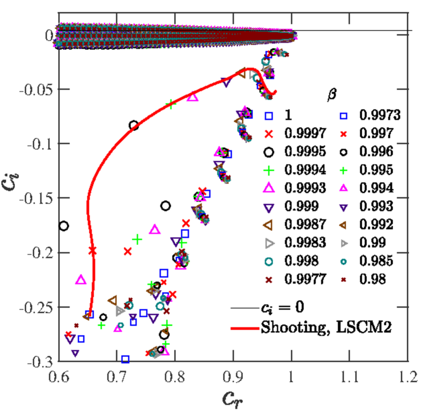
(a) $(1-\beta)\in 0$ to $0.02$

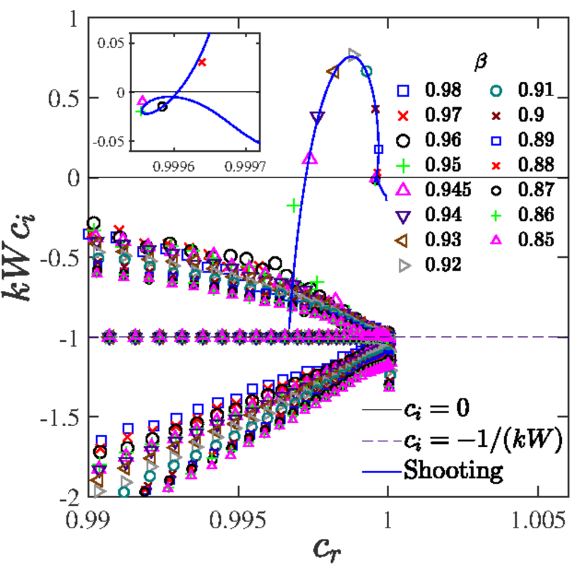
(b) $(1-\beta)\in 0.02$ to $0.15$

Figure 12: Viscoealstic pipe flow eigenspectra for $E=0.15,\Rey=6000,k=1$, and for varying $\beta$ (a) $(1-\beta)=0$ to $0.02$, and (b) $(1-\beta)=0.02$ to $0.15$. Panel (a) shows the region in the vicinity of the $P$-branch. Panel (b) focuses on the trajectory of the center mode which becomes unstable for $\beta\in(0.88,0.945)$.

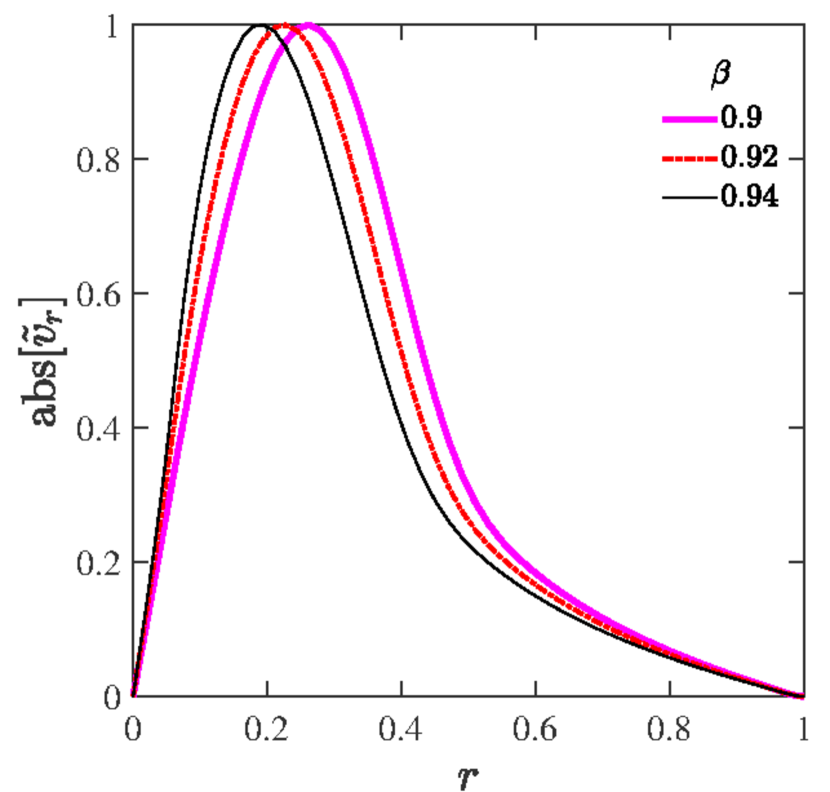
(a) Radial velocity

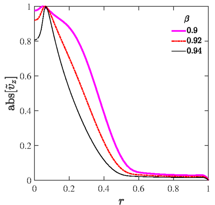
(b) Axial velocity

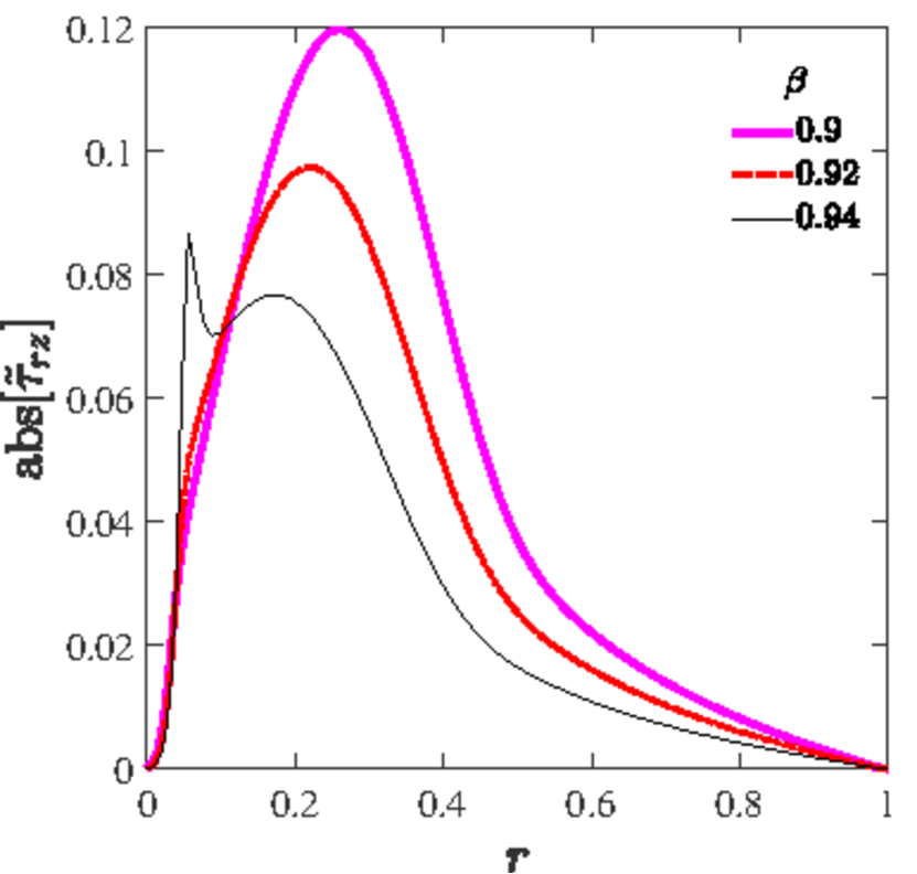
(c) $T_{rz}$ stress

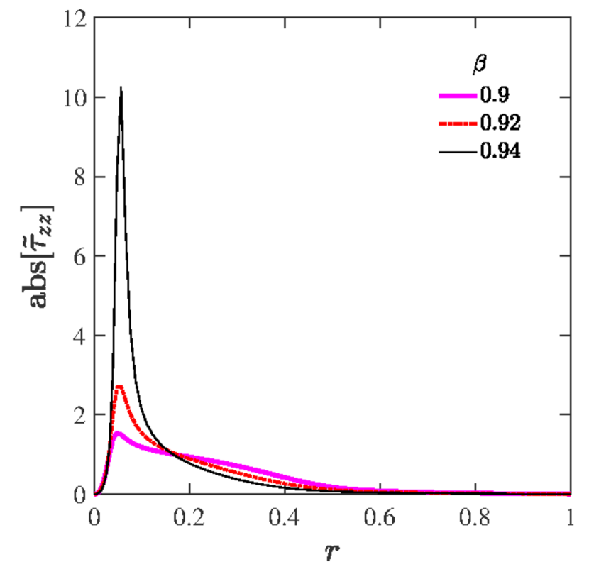
(d) $T_{zz}$ stress

Figure 13: Velocity and polymer stress eigenfunctions corresponding to the unstable centre modes (in Fig. 12(b)) at different $\beta$ for $E=0.15,\Rey=6000$ and $k=1$.

In Fig. 12, we show the eigenspectra (overlaid) as $\beta$ is reduced from unity, again at fixed $E$, $Re$ and $k$; note that the $\beta$’s shown are all higher than the threshold value for collapse into the CS (the analogue of that identified in Fig. 9(a), but for $Re=6000$). Figure 12(a) is for $\beta$’s close enough to unity that the center mode has not emerged out of the CS yet (the other stable modes, with $c_{r}\rightarrow 0$, are not shown). Thus, the trends in this figure pertain to all other (least stable) modes on the P branch. Figure 12(a) shows no discernible trend in the behaviour of the P branch modes with changing $\beta$. For instance, as $\beta$ is decreased, the least-stable Newtonian mode moves in the clockwise sense in $(c_{r},c_{i})$-plane. In contrast, the mode LSCM2 smoothly continues from a Newtonian mode at the junction of the ’APS’ structure present at $\beta=0$. The remaining modes are, however, smooth continuations of the modes of the Newtonian $P$ branch, but these move in the counter-clockwise sense with decreasing $\beta$. Eigenspectra for smaller $\beta$ in the interval $0.85\leq\beta\leq 0.98$ are shown in Fig. 12(b), the focus being on the center mode. The center mode first emerges at $\beta=0.96$, and becomes unstable for $\beta\in[0.88,0.945]$. The smooth (blue) curve, passing through the spectral center mode eigenvalues, shows the trajectory of the center mode with decreasing $\beta$, obtained using the shooting method. Thus, at a fixed $E$, the unstable center mode always emerges out of the CS as $\beta$ is decreased from unity.

The velocity and stress eigenfunctions corresponding to some of the unstable center modes in Fig. 12(b) are shown in Fig. 13. For the higher $\Rey$ ($=6000$), the axial velocity eigenfunctions are more localized near the center (as $\beta$ approaches unity), compared to those for $\Rey=600$ shown in Fig. 6(b). The axial stress $T_{zz}$ (Fig. 13(d)) shows a sharp peak as $\beta$ approaches unity at fixed $E$, similar to the feature that was seen earlier (Fig. 6(d)), albeit with decreasing $E$ at a fixed $\beta$ for $Re=600$. For the values of $\beta$ examined here, both the axial and radial eigenfunctions exhibit a rather smooth variation with $r$, unlike the rapid, oscillatory variation (not shown) characteristic of wall modes ($c_{r}\rightarrow 0$) for $\beta\rightarrow 0$. The latter are analogous to wall modes in viscoelastic channel flow whose structures was examined in detail by Chaudhary et al. (2019) (see Fig. 20 therein); the overall similarity of the pipe and channel flow UCM spectra was already discussed above.

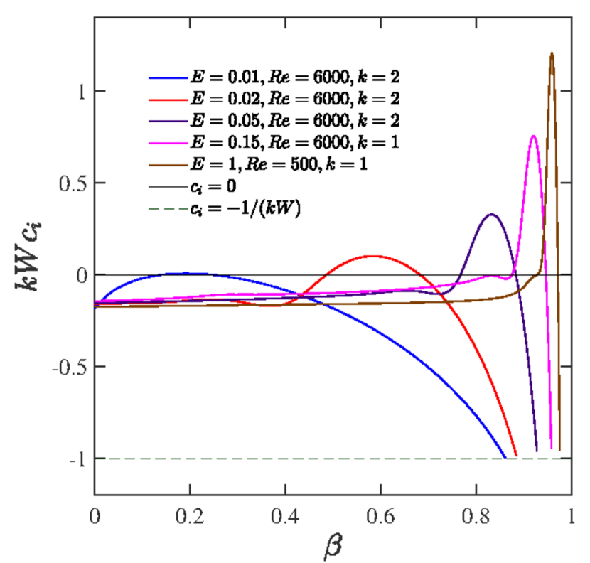
(a) Growth rate

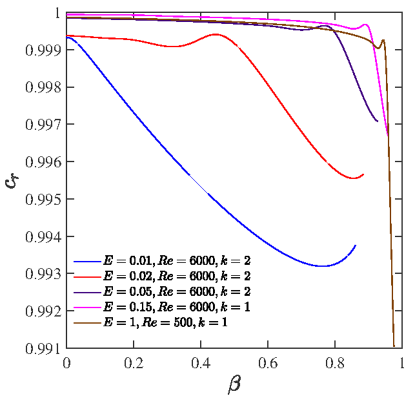
(b) Phase speed

Figure 14: (a) Scaled growth rate and (b) phase speed, for the center mode, with varying $\beta$, for different fixed sets of parameters $(E,\Rey,k)=(0.01,6000,2),(0.02,6000,2),(0.05,6000,2),(0.15,6000,1)$ and $(1,500,1)$.

3.2.1 The origin of the center mode at fixed $E$ and varying $\beta$

While the discussion pertaining to Fig. 12(b) showed that center mode emerges out of the CS as $\beta$ is decreased from unity, in Fig. 14(a), we address the question of what happens as $\beta$ is decreased down to zero (the UCM limit). This figure shows the variation of the scaled growth rate, $kWc_{i}$, of the center mode with varying $\beta$ at fixed $Re$, $E$ and $k$. As $\beta$ is decreased from unity, the center mode emerges out of CS1 (when $kWc_{i}=-1$) at a critical $\beta$, and becomes unstable as $\beta$ is decreased further. The critical $\beta$ corresponding to the emergence of the center mode is closer to unity for higher $E$. The range of unstable $\beta$ also approaches unity for larger $E$, while also narrowing down in extent, with a concomitant increase in the growth rate. A similar narrowing down occurs when $E$ approaches the lower threshold for the instability, for the chosen $\beta$ (the blue curve in Fig. 14(a)). Figure 14(b) shows that the corresponding $c_{r}$ remains close to (and less than) unity for the entire range of $\beta$.

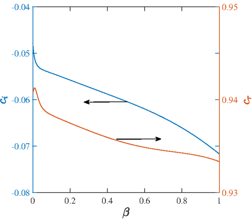
(a) Growth rate and Phase speed

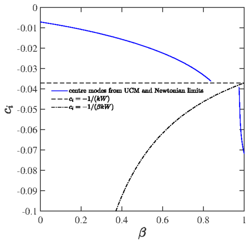
(b) Growth rate

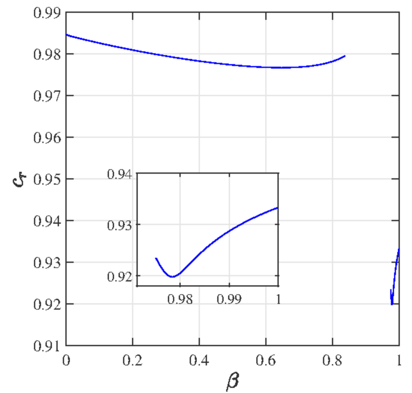
(c) Phase speed

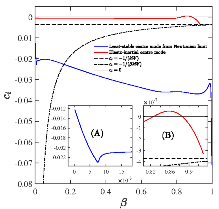
(d) Growth rate

(e) Phase speed

Figure 15: The three possible center mode trajectories with variation in $\beta$ for $\Rey=600,k=3$ at various fixed values of the elasticity number: $E=0.005$ in panel (a), $E=0.015$ in panels (b) and (c), and $E=0.15$ in panels (d) and (e). Insets $(A)$ in panels (d) and (e) show the enlarged regions near $\beta=0$ and $\beta=1$, respectively. Inset $(B)$ in panels (d) show the enlarged views of the unstable range of $\beta$s.

In Fig. 15, we show the three possible behaviours, within the parameter regimes explored, for the trajectory of the least stable center mode as $\beta$ is varied from the UCM to the Newtonian limit. For the smallest elasticities (e.g., $E=0.005$ in Fig. 15(a)), when the two CS are highly stable, and well outside the range of $c_{i}$’s shown, the center mode, while remaining stable, smoothly continues all the way from the UCM limit ($\beta=0$) to the Newtonian ($\beta=1$) limit without suffering any discontinuities or abrupt endings. For moderate elasticities (e.g., $E=0.015$ shown in Fig. 15(b)), the $c_{i}$ vs $\beta$ curve for the least stable center mode starts from the Newtonian end ($\beta=1$), but abruptly ends as it encounters CS2 from below. On the other hand, the least stable center mode in the UCM limit continues to finite $\beta$, abruptly ending at the location of its encounter with CS1 from above. Corresponding phase speeds for $E=0.015$ are shown in Fig. 15(c), with the inset showing an enlarged view near $\beta=1$, where the variation of the phase speed $c_{r}$ with $\beta$ is quite sharp. For the chosen parameters, the center mode still remains stable for all $\beta$. Finally, for higher elasticity (e.g., $E=0.15$), the $c_{i}$ vs $\beta$ curve for the least-stable mode from the Newtonian end continues all the way up to the UCM limit without suffering discontinuities as shown in Fig. 15(d), ending up as a center mode in the UCM spectrum. Inset (A) shows a magnified view of the sharp variation of the $c_{i}$ curve near $\beta=0$. The least stable center mode in the UCM limit behaves similar to the previous case of $E=0.015$, with an abrupt ending as it collapses onto CS1 from above, the only difference now being that the mode is unstable for a small range of $\beta$ (due to the higher $E$); inset (B) provides the enlarged view of the unstable range of $\beta$. The corresponding phase speeds for $E=0.15$ are shown in Fig. 15(e) with inset (A) showing the enlarged view of the non-monotonic behaviour near the Newtonian limit. Note that the Newtonian center mode does not suffer a jump despite crossing the CS2 curve ($c_{i}=-1/(\beta kW)$) in Fig. 15(d); this is only an apparent crossing since, as shown in Fig. 15(e), its phase speed exceeds unity, and it therefore ‘goes around’ CS2 with decreasing $\beta$. In contrast, the discontinuities in the center mode trajectory, in Fig. 15(b), occur because $0<c_{r}<1$.

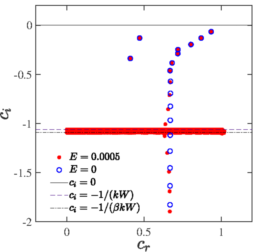
(a) $E=0.0005$

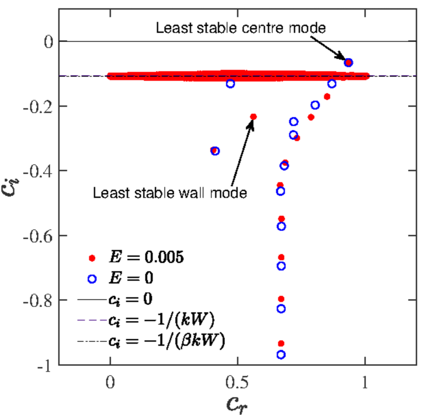
(b) $E=0.005$

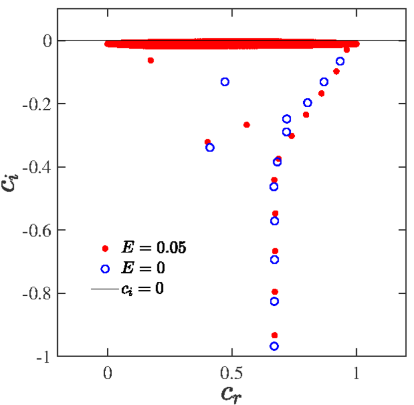
(c) $E=0.05$

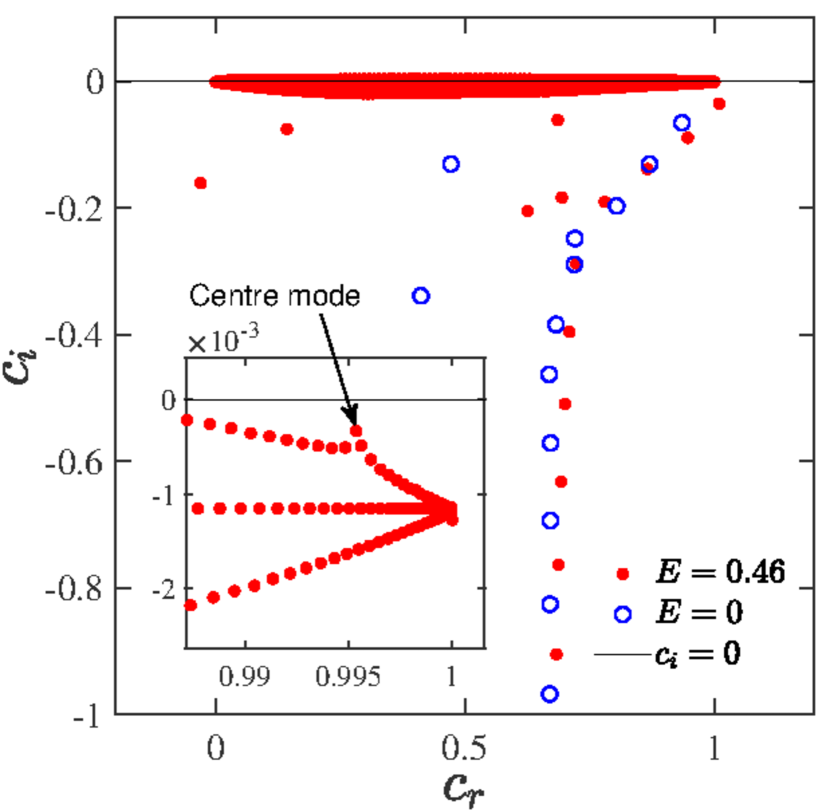
(d) $E=0.46$

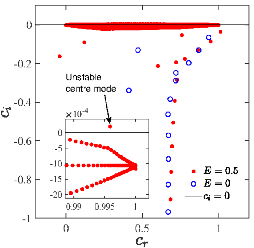
(e) $E=0.5$

Figure 16: Viscoelastic pipe-flow eigenspectra at $\beta=0.97$ for different $E$: (a) $0.0005$, (b) $0.005$, (c) $0.05$, (d) $0.46$, and (e) $0.5$, compared with the Newtonian eigenspectrum ($E=0$), for $\Rey=1500$ and $k=0.4\pi$.

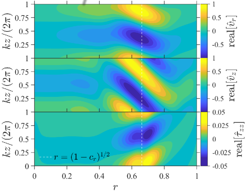
(a) Least-stable wall mode

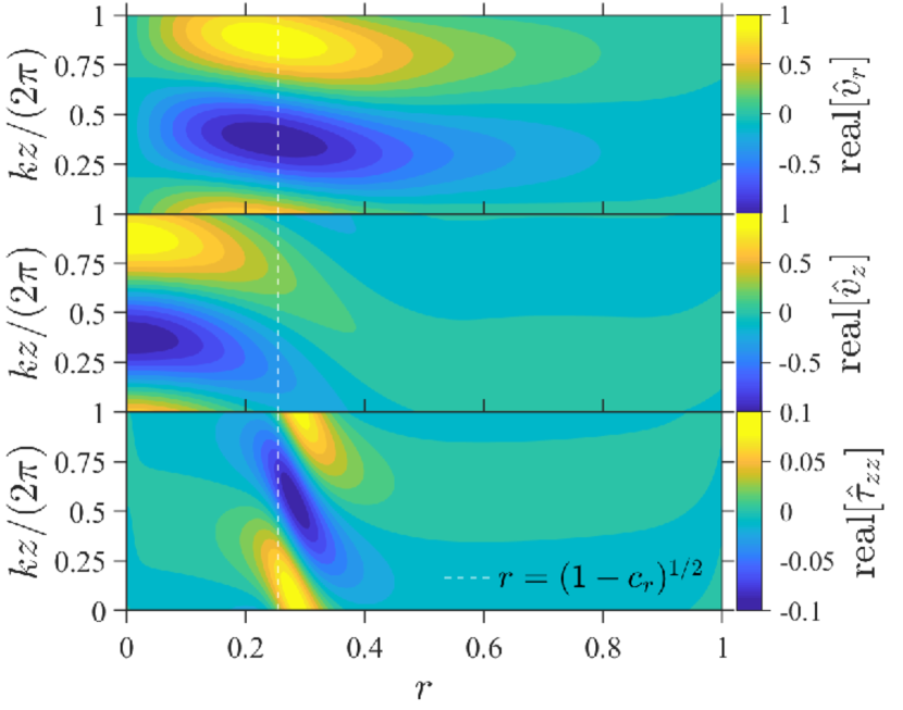
(b) Least-stable centre mode

Figure 17: Contours of the radial ($\hat{v}_{r}$), axial ($\hat{v}_{x}$) velocities and axial normal stress ($\hat{\tau}_{zz}$) in the $r$–$z$ plane for the least stable wall and centre modes (marked in Fig. 16(b)) in pipe flow for $E=0.005,\beta=0.97,\Rey=1500$ and $k=0.4\pi$: (a) Least-stable wall mode $c=0.561844626-0.233038878\mathrm{i}$ from the A-branch of the eigenspectrum, and (b) for the least-stable centre mode $c=0.935239154-0.064928230\mathrm{i}$ from the P-branch of the eigenspectrum. The location of the critical layer is shown using white dashed lines.

3.3 Center vs. wall modes in viscoelastic pipe and channel flows

In the results presented so far, we have characterized the behaviour of the elasto-inertial center mode as a function of $E$ and $\beta$. Although this mode may either be directly related to a Newtonian center mode (for $\beta$’s below a threshold), or be disconnected from the Newtonian spectrum (for $\beta$’s above), the interpretation is nevertheless that the elasto-inertial turbulence observed in recent experiments (Samanta et al., 2013; Choueiri et al., 2018; Chandra et al., 2018) is the outcome of a linear instability associated with this center mode. In sharp contrast to this picture, in a recent effort, Shekar et al. (2019) have argued based on DNS simulations and a singular-value decomposition analysis that elasto-inertial turbulence in channel flow might instead be closely related to the elastically modified TS mode. As is well known, the TS mode is the least stable wall mode in the Newtonian limit, and this remains true for the range of elasticities considered by the authors. Thus, the premise of Shekar et al. (2019) continues to be along the lines of a sub-critical bifurcation to EIT, similar in spirit to the earlier efforts of Meulenbroek et al. (2003); Morozov & van Saarloos (2005, 2007) in the inertialess limit, and to the work of Stone et al. (2002); Stone & Graham (2003); Stone et al. (2004); Li & Graham (2007) based on an elastic modification of 3D ECS structures. The main difference is that the bifurcation ascribed by Shekar et al. (2019) is supposedly to a finite amplitude 2D mode, with EIT-like dynamics. The authors reported results for $\Rey=1500$ (where the Newtonian flow is turbulent), $\beta=0.97$, and for $0<W<50$. It is worth noting that, for these parameters, the elastically modified ECS’s originally examined by Graham and co-workers (Li & Graham, 2007) also exist, although Shekar et al. (2019) restrict themselves to two-dimensional initial conditions.

While the present study is restricted to linear (modal) stability of pipe flow of an Oldroyd-B fluid, it is nevertheless instructive to compare the viscoelastic pipe and channel flow spectra in order to assess the relative importance of center and wall modes in these geometries. Such an assessment would help set the template (in terms of the relevant linear modes, both discrete and continuous) for a nonlinear bifurcation analysis. We show representative eigenspectra for pipe flow (in Fig. 16) for a range of $E$ that subsumes the range ($0<E<0.013$) considered by Shekar et al. (2019), for $\beta=0.97,\Rey=1500$ and $k=0.4\pi$. In each panel, the corresponding Newtonian spectrum is also shown for comparison (as open blue circles). For $0.0005<E<0.05$, with increasing $E$, discrete modes collapse into the CS, and new ones emerge from below, similar to what was shown in Fig. 3. The center mode emerges from CS1 at $E=0.46$, (see inset of Fig. 16(d)), becoming unstable at $E\approx 0.5$ (Fig. 16(e)). Importantly, for the parameters considered in Fig. 16, the center mode always remains the least stable or unstable mode. This feature remains true even for other regimes investigated in this study ($\Rey\in 100$–$2000$). This is unlike Newtonian channel flow, where there is a range of parameters where the wall mode (i.e., the TS mode) is the least stable (or unstable), and this remains true for small but finite $E$.

An important feature of Newtonian pipe flow is the absence of a critical-layer singularity (Drazin & Reid, 1981; Schmid & Henningson, 2001) for axisymmetric disturbances, as a result of which there is no axisymmetric analogue of the two-dimensional TS instability. This difference between pipe and channel flows appears to persist even in the presence of elasticity. In Fig. 17, we show, via contour plots, the spatial structure of the least stable center and wall modes marked in Fig. 16(b). Further, and in sharp contrast to viscoelastic channel flow, where the elastically-modified TS mode was shown to have the $T_{xx}$ (the stream-wise component of the normal stress) eigenfunction strongly localized in the critical layer (see Fig. 2 of Shekar et al. (2019)), neither the least stable center nor the wall mode in pipe flow exhibits a comparably strong localization of $T_{zz}$; in fact, the extent of localization is more stronger for the center mode. For these reasons, the connection between the (stable) TS wall mode to the elasto-inertial structures suggested by Shekar et al. (2019) (in the context of viscoelastic channel flow) is not applicable for viscoelastic pipe flow. This aspect will be discussed in more detail in a future communication (Khalid et al., 2020), where we show that, even for viscoelastic channel flows, the parameter regime relevant to the proposed TS-mode-based subcritical mechanism of Shekar et al. (2019) is somewhat restricted. It is worth emphasizing that all of the experiments on viscoelastic transition (with the exception of Srinivas & Kumaran, 2017) pertain to the pipe geometry. Further, and importantly, recent simulations in both the channel (Samanta et al., 2013; Sid et al., 2018) and pipe (Lopez et al., 2019) geometries have found analogous (span-wise oriented) coherent structures, suggesting a common underlying mechanism for elasto-inertial transition.

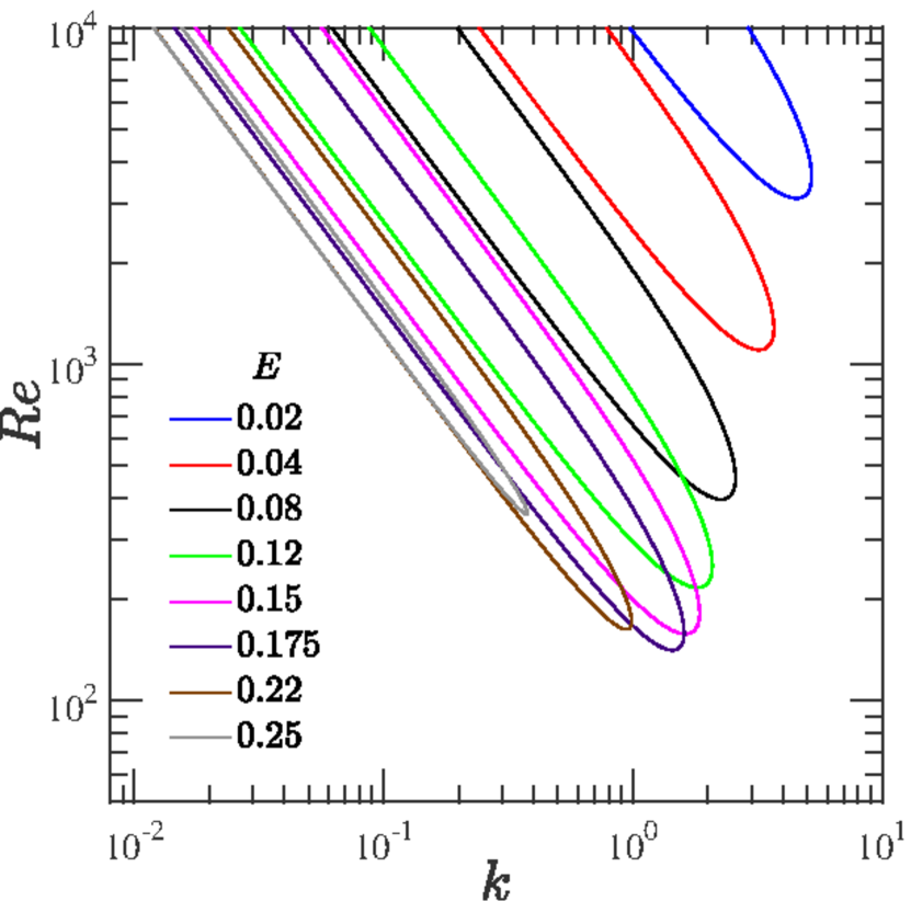
(a) $\beta=0.65$

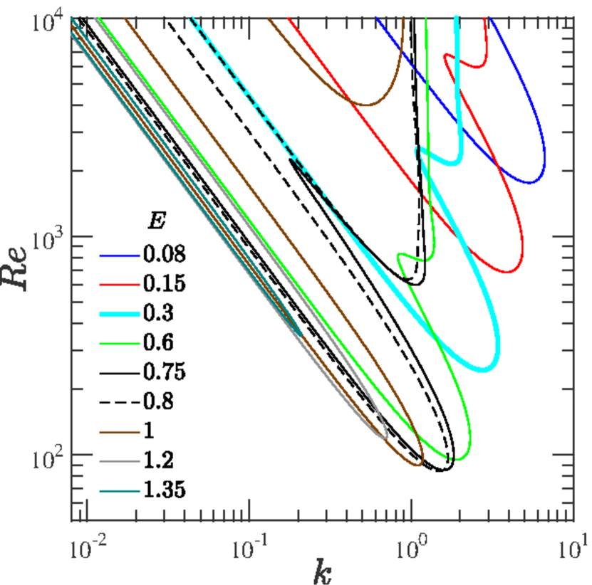
(b) $\beta=0.9$

Figure 18: Neutral stability curves in the $Re$–$k$ plane for varying $E$ at: (a) $\beta=0.65$, and (b) $\beta=0.9$.

4 Neutral stability curves

Figures 18(a) and 18(b) show the neutral stability curves in the $Re$-$k$ plane for fixed $\beta$ and $E$. The curves are in the form of loops, with the region inside the loop being unstable. While $Re\sim 1/k$ for $k\ll 1$ in the lower and upper branches of the loop for the smaller $\beta$ ($=0.6$), the upper branch behaves in a different manner for $\beta=0.9$. In Fig. 18(b), the upper branch has a non-monotonic behaviour as $E$ is increased, with a secondary minimum emerging at a higher $\Rey$. This feature of multiple minima is reminiscent of a similar phenomenon observed, albeit for wall modes, in the UCM limit for plane channel flow (see Fig. 15 of Chaudhary et al., 2019). The two minima move apart with increasing $E$, and for $E=0.8$ and higher, the junction of the two distinct lobes in a given neutral curve moves out of the range of $\Rey$ examined. Thus, the neutral curves for $E\geq 0.8$ appear as a pair of disconnected envelopes. Both branches of the lower envelope exhibit the aforementioned $1/k$ scaling for small $k$. In contrast, only the lower branch of the upper envelope exhibits this scaling, with the upper branch being almost vertical (Fig. 18(b)). The phase speeds corresponding to the neutral curves shown in Figs. 18(a) and 18(b) are shown in Figs. 19(a) and 19(b) respectively. Overall, the phase speeds always remain close to, but less than, unity (the maximum base-flow velocity). For the higher $\beta$, $c_{r}$ varies in a narrower range close to unity, approaching it more closely at the higher $E$ (Fig. 19(b)), but never exceeding unity. Thus, the center mode character of the instability is preserved all along the neutral curves. Similar to the two-lobed structure of the neutral curves in the $Re$–$k$ plane for $\beta=0.9$ (Fig. 18(b)), a corresponding two-lobed structure is seen in the $c_{r}$–$k$ plane as well for $E\approx 0.15$ onwards.

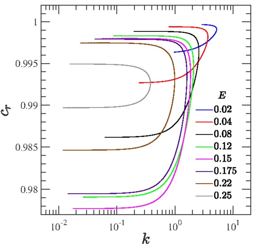
(a) $\beta=0.65$

(b) $\beta=0.9$

Figure 19: The variation of the phase speed, as a function of $k$, corresponding to the neutral curves for different $E$ in Fig. 18 at two different values of $\beta$.

For a given $E$ and $\beta$, the minimum of the neutral curve (the global one when there are multiple lobes) is the critical Reynolds number ($\Rey_{c}$), the lowest Reynolds number at which the flow is unstable. We mainly focus on the lower curve only, because the critical Reynolds number $\Rey_{c}$ lies on it. To begin with, an increase in $E$ shifts the neutral curves to lower $\Rey$ and $k$, but beyond a certain critical $E$, the neutral curves again shift towards higher $\Rey$. Interestingly, the minima of the neutral curves are $O(100)$ for sufficiently high $E$ (as first reported in our Letter; Garg et al., 2018), as opposed to a typical $\Rey$ of $O(2000)$ for the Newtonian transition.

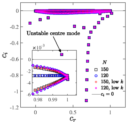
Figure 20: Comparison of the (unfiltered) asymptotic small-$k$ eigenspectrum with that obtained from the full problem for $\beta=0.9,E=0.15,k=0.3$ and $\Rey=8000$. Inset shows the zoomed region near the unstable mode.

The $\Rey\propto k^{-1}$ scaling followed by the lower branches of the neutral curves in Fig. 18 suggests a regular perturbation analysis in the $k\ll 1$ limit wherein Eqs. 13–19 can be simplified by systematically neglecting terms of $O(k)$ or higher. From the neutral curves at fixed $E$, one obtains $\Rey=k^{-1}\tilde{\Rey}$, $W=k^{-1}\tilde{W}$ for the $k$-scalings of the dimensionless parameters. The radial velocity may be expanded as:

$$\tilde{v}_{r}\equiv\tilde{v}_{r}^{(0)}+k\tilde{v}_{r}^{(1)}+k^{2}\tilde{v}_{r}^{(2)}+...\,,$$ (20)

which, when substituted in the continuity, $z$-momentum, $rr$-, $rz$- and $zz$-stress equations, i.e., Eqs. 13, 15–17 and 19, yields the following scalings at leading order:

$$\left.\begin{array}[]{ll}\displaystyle\tilde{v}_{r}\sim\tilde{v}_{r}^{(0)},\quad\tilde{v}_{z}\sim k^{-1}\tilde{v}_{z}^{(0)},\quad\tilde{p}\sim k^{-1}\tilde{p}^{(0)},\\[8.0pt] \displaystyle\tilde{\tau}_{rr}\sim k\tilde{\tau}_{rr}^{(0)},\quad\tilde{\tau}_{rz}\sim\tilde{\tau}_{rz}^{(0)},\quad\tilde{\tau}_{zz}\sim k^{-1}\tilde{\tau}_{zz}^{(0)},\end{array}\right\}$$ (21)

The above scalings are used in Eqs. 13–15 to obtain the following simplified set of equations, to leading order in $k$:

$$(\mathrm{D}+\frac{1}{r})\tilde{v}_{r}^{(0)}+\mathrm{i}\tilde{v}_{z}^{(0)}=0,$$ (22)

$$\mathrm{D}\tilde{p}^{(0)}=0,$$ (23)

$$-U^{\prime}\tilde{v}_{r}^{(0)}+\{\frac{\beta}{\tilde{\Rey}}(\mathrm{D}^{2}+\frac{\mathrm{D}}{r})-\mathrm{i}(U-c)\}\tilde{v}_{z}^{(0)}-\mathrm{i}\tilde{p}^{(0)}+(\mathrm{D}+\frac{1}{r})\tilde{\tau}_{rz}^{(0)}+\mathrm{i}\tilde{\tau}_{zz}^{(0)}=0.$$ (24)

The boundary conditions become:

$$\left.\begin{array}[]{ll}\displaystyle\tilde{v}_{r}^{(0)}=0=\tilde{v}_{z}^{(0)}\quad\mbox{at\ }\quad r=1,\\[8.0pt] \displaystyle\tilde{v}_{r}^{(0)}=0,\tilde{v}_{z}^{(0)}=\text{ finite, }\tilde{p}^{(0)}=\text{ finite}\quad\mbox{at \ }\quad r=0,\end{array}\right\}$$ (25)

The simplified system comprising Eqs. 22–24 was solved using a spectral method and the eigenspectrum obtained is compared with that for the full problem at $k=0.3$ for the same parameters (Fig. 20); the inset zooms in on the unstable center mode. Both eigenspectra have a similar structure, and in particular, the center mode obtained from the low-$k$ analysis has the same phase speed and growth rate as that in the original problem.

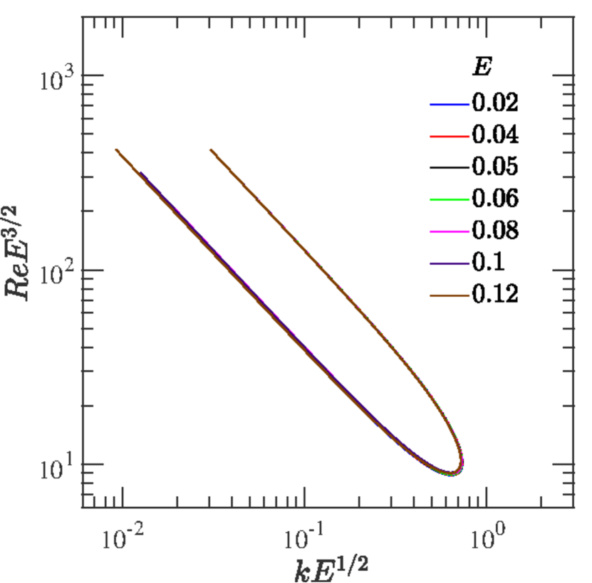
(a) Rescaled neutral curves for $\beta=0.65$

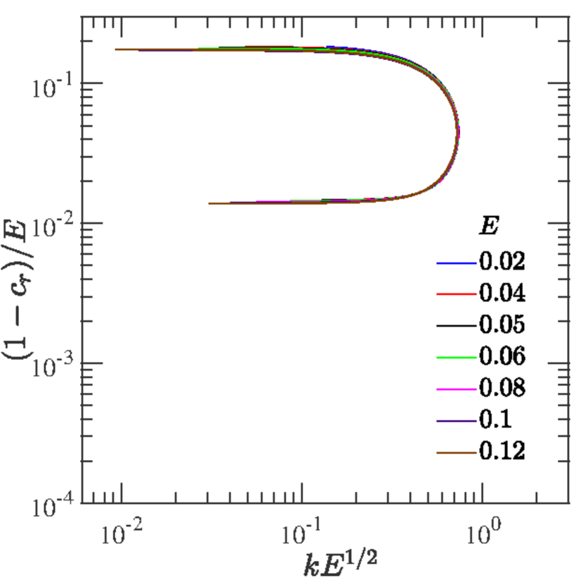
(b) $(1-c_{r})$ collapse for $\beta=0.65$

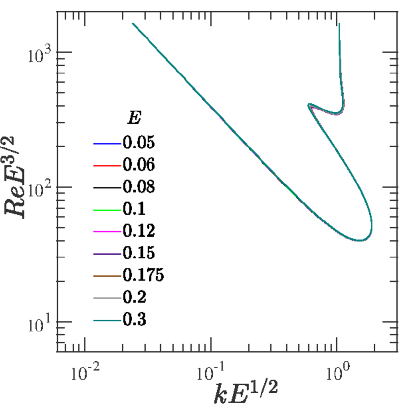
(c) Rescaled neutral curves for $\beta=0.9$

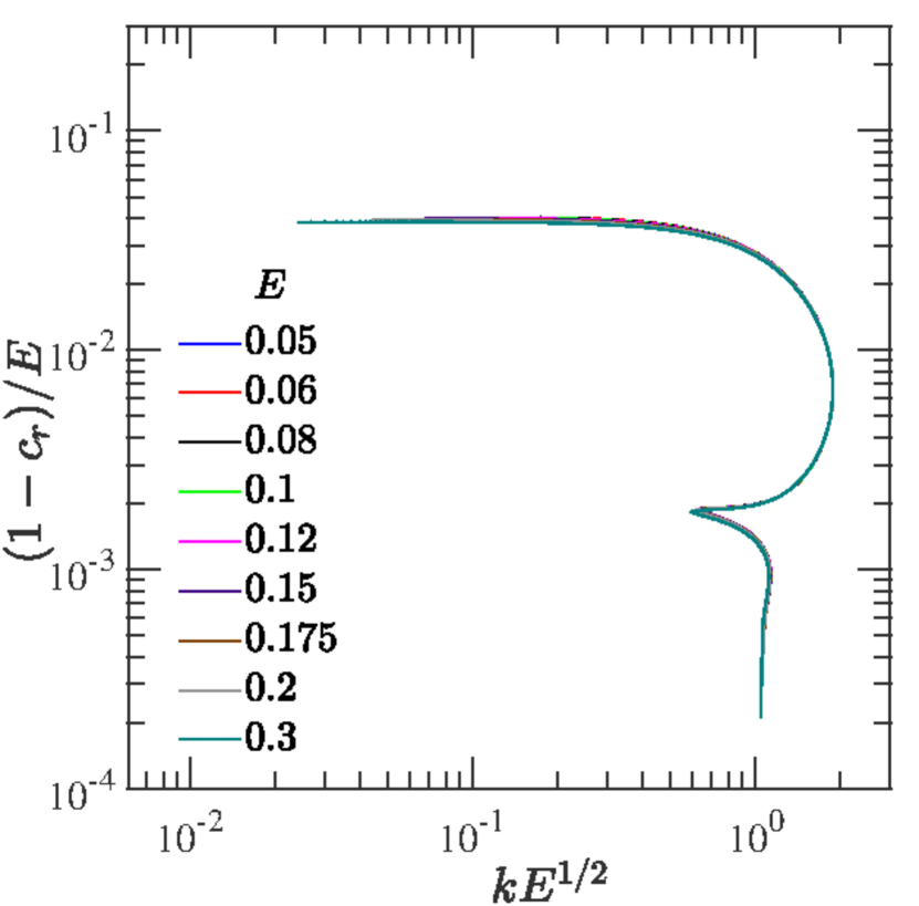
(d) $(1-c_{r})$ collapse for $\beta=0.9$

Figure 21: Collapse of neutral curves for different $E$ in the $Re$-$k$ plane (panels (a) and (c)) and collapse of the corresponding phase speeds (panels (b) and (d)) for two different $\beta$.

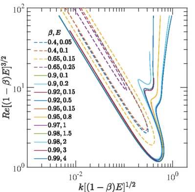
Figure 22: Neutral curves for different $\beta$ and $E$ plotted in terms of $\Rey[(1-\beta)E]^{3/2}$ vs. $k[(1-\beta)E]^{1/2}$: The rescaled neutral curves collapse for $\beta\rightarrow 1$.

4.1 Collapse of neutral curves

The qualitatively similar character of the neutral curves at different $E$ in Fig. 18 is strongly suggestive of a collapse upon suitable rescaling of both $\Rey$ and $k$ with the elasticity number $E$. Figure 21 shows that such a collapse is indeed possible for sufficiently small $E$, when $Re$ is rescaled as $\Rey E^{3/2}$ and $k$ as $kE^{1/2}$. These scalings are found to be valid for fixed $\beta$, although the nature of the collapsed curve does depend on $\beta$ (as evident from Figs. 21(a) and 21(c)). Similarly, as shown in Figs. 21(b) and 21(d), the curves for the rescaled phase speed $(1-c_{r})/E$, plotted as a function of $kE^{1/2}$, again exhibit a collapse, implying that $(1-c_{r})$ is $O(E)$ for $E\ll 1$.

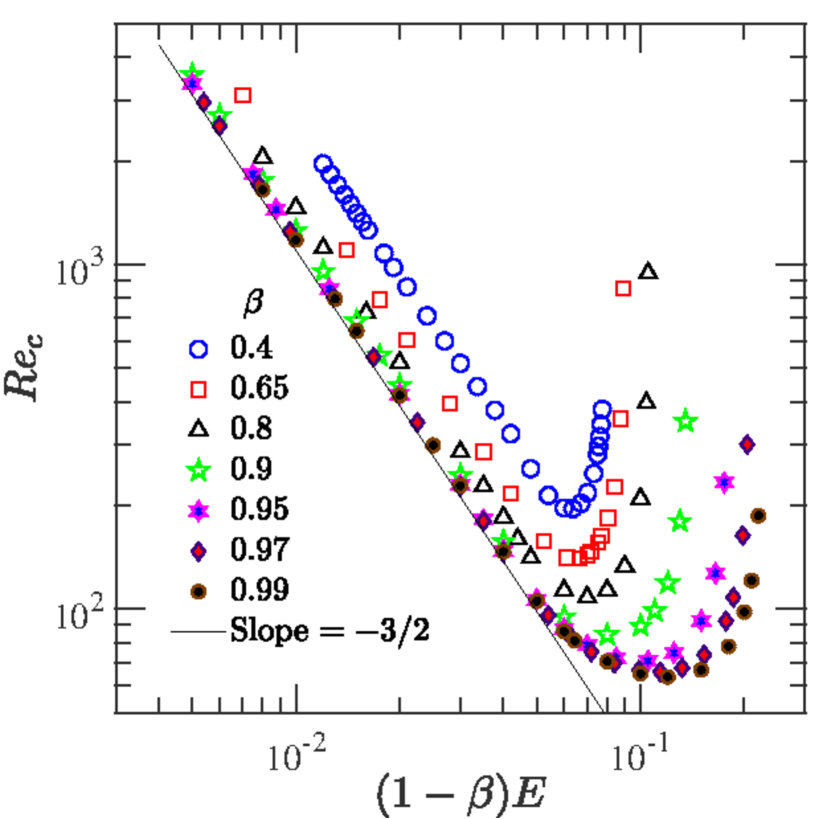
(a) $Re_{c}$ vs. $E(1-\beta)$

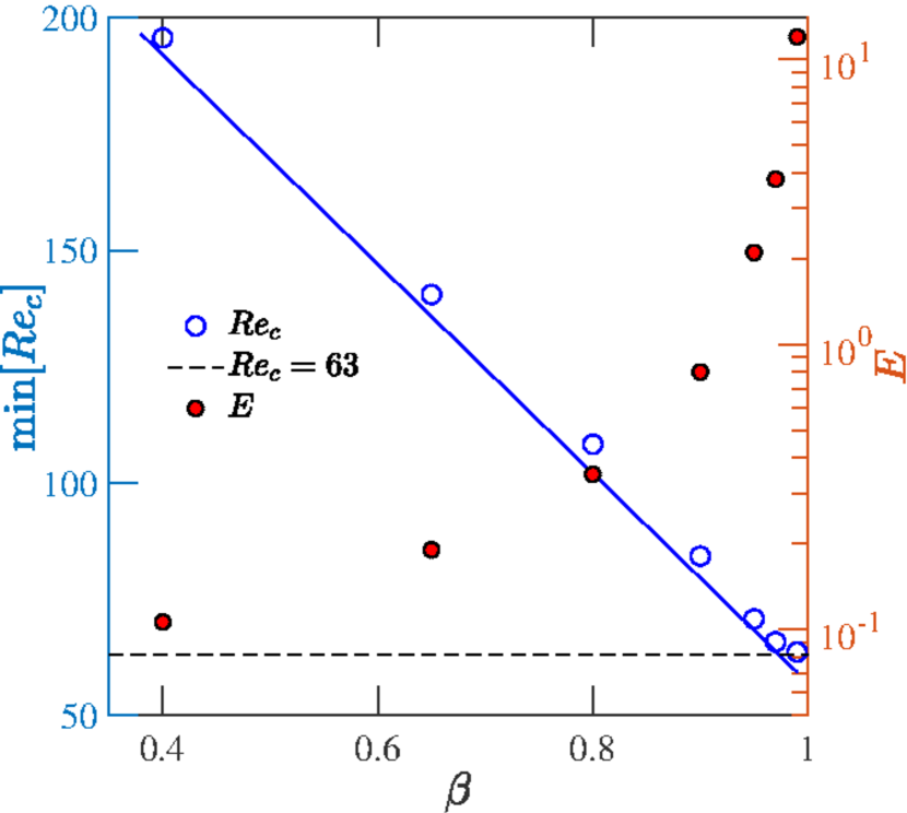
(b) $\mathrm{min}[\Rey_{c}]$ vs $\beta$

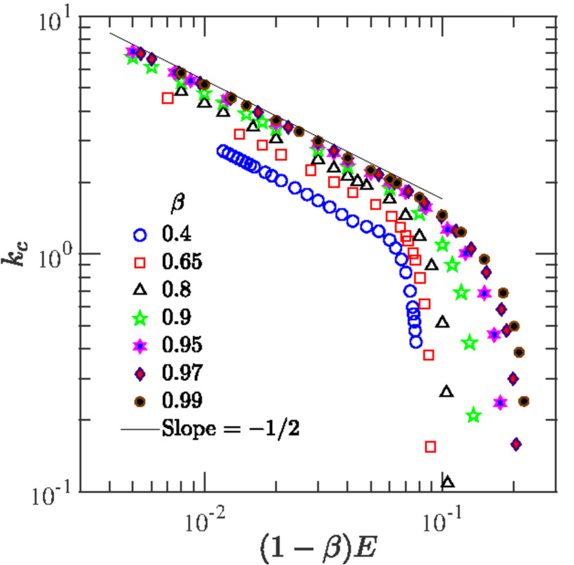
(c) $k_{c}$ vs $E(1-\beta)$

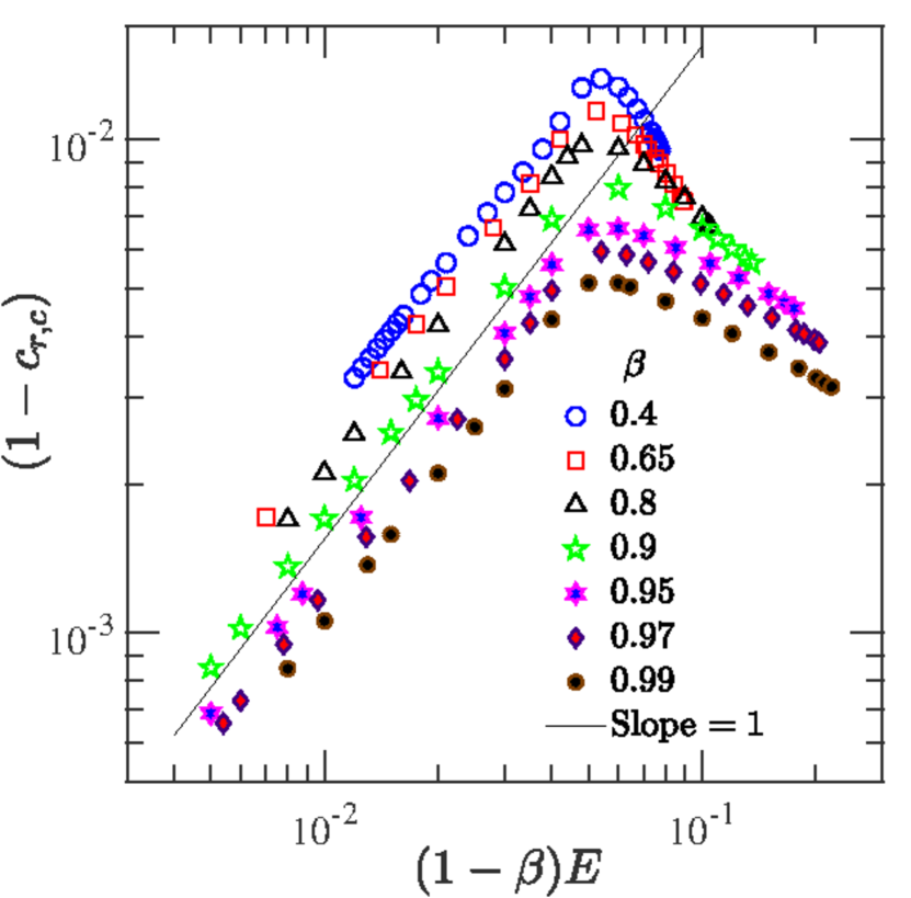
(d) $(1-c_{r,c})$ vs $E(1-\beta)$

Figure 23: Variation of critical parameters with $E(1-\beta)$ for $\beta$ ranging from $0.4$ to $0.99$. (a) $Re_{c}$ vs $E(1-\beta)$, (b) The minima of $\Rey_{c}$ of panel (a) decreases approximately in a linear manner with $\beta$, but appears to approach a finite value as $\beta\rightarrow 1$, while the corresponding $E$ diverges as $\beta\rightarrow 1$, (c) $k_{c}$ vs $E(1-\beta)$, and (d) $(1-c_{r,c})$ vs $E(1-\beta)$. $\Rey_{c}$ and $k_{c}$ follow the scalings $Re_{c}\propto[E(1-\beta)]^{-3/2}$ and $k_{c}\propto[E(1-\beta)]^{-1/2}$ respectively below a critical value of $E(1-\beta)$.

While the collapse obtained above is for a fixed $\beta$ and for $E\ll 1$, a further collapse is obtained in the dual limit $E(1-\beta)\ll 1$, $(1-\beta)\ll 1$, when the neutral curves are plotted in terms of $\Rey[(1-\beta)E]^{3/2}$ and $k[(1-\beta)E]^{1/2}$ as shown in Fig. 22, implying that the threshold $\Rey$ and $k$ scale as $\Rey\propto[(1-\beta)E]^{-3/2}$ and $k\propto[(1-\beta)E]^{-1/2}$ respectively, in this limit. The rescaled neutral curves in Fig. 22 begin to collapse onto a single one only for $\beta>0.9$, the collapse being perfect for the lower branch, but less so for the upper ones. Thus, the role of the solvent viscosity appears to be ‘universal’ only as far as the lower branch is concerned. Importantly, however, since the critical $Re$ occurs on the lower branches of the neutral curves, the transition to the elasto-inertial turbulent state is governed by the combination $E(1-\beta)$ for $E(1-\beta)\ll 1$, $(1-\beta)\ll 1$. It is worth noting that the nearly-vertical nature of the upper branch implies that the instability appears to exist in the limit of $\Rey\rightarrow\infty$, with $E$ fixed. An axisymmetric version of the ‘elastic Rayleigh’ equation (the elastic analogue of the classical Rayleigh equation; see Rallison & Hinch, 1995; Subramanian et al., 2020), which also has $E(1-\beta)$ as the governing parameter, is known to govern the linearized dynamics of perturbations in this limit, and involves a balance of inertial and elastic forces in the fluid. There is, however, no instability associated with the elastic Rayleigh equation for plane- (Kaffel & Renardy, 2010) and pipe-Poiseuille (Chaudhary et al., 2020) flows, and the lack of collapse of the (near-vertical) upper branches, and the implied instability for $Re\rightarrow\infty$, in Fig. 22, betrays therefore the singular nature of the inviscid elastic limit, with viscous effects playing a likely role even as $Re\rightarrow\infty$.

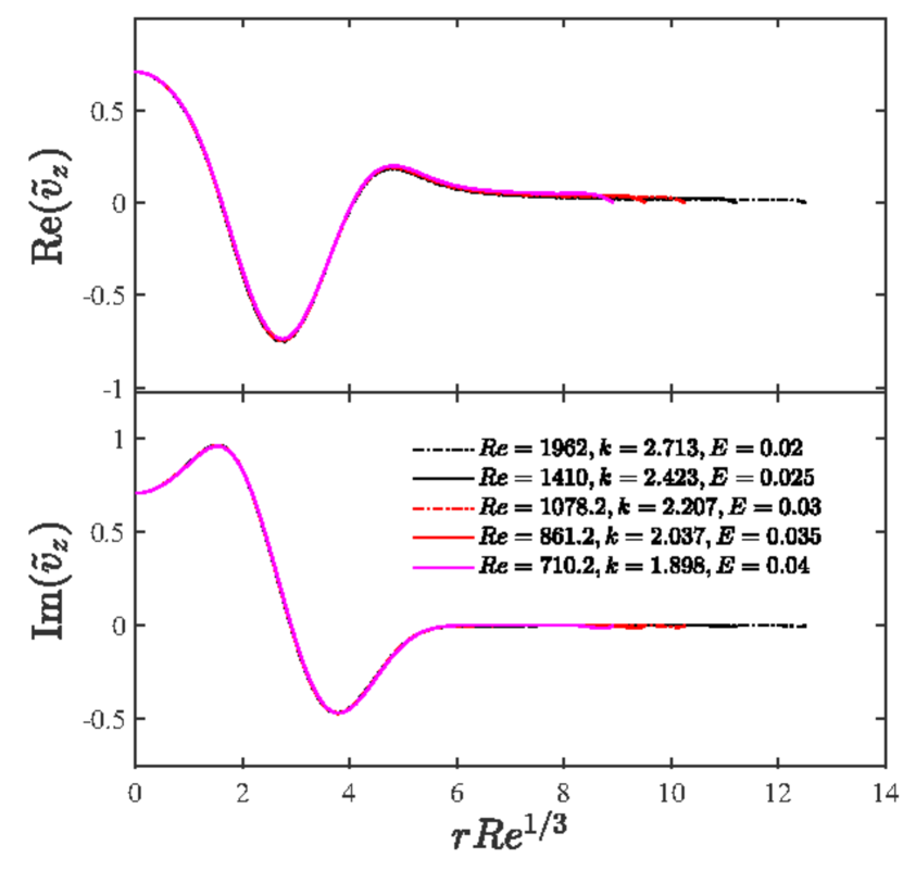
(a) $\tilde{v}_{z}$

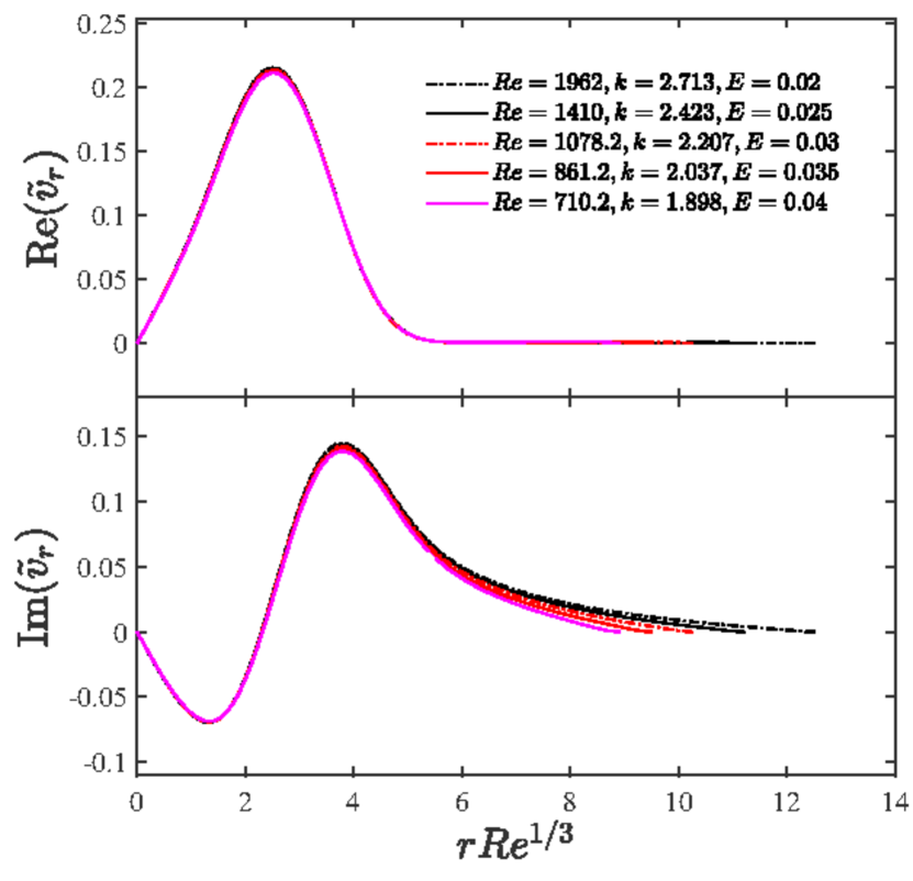
(b) $\tilde{v}_{r}$

Figure 24: Collapse of eigenfunctions at different $\Rey$ and $k$ along the lower branch of the neutral curve for $\beta=0.4$. The eigenvalues (with $c_{i}=0$) for which the rescaled eigenfunctions are shown are $c=0.996707,0.995912,0.995131,0.994367$ and $0.993621$ respectively.

4.2 Critical parameters and scalings

Figures 23(a), 23(c) and 23(d) show the variation of critical parameters $\Rey_{c}$, $k_{c}$ and $c_{r,c}$ with $E(1-\beta)$ for different $\beta$. Irrespective of $\beta$, the critical parameters conform to scaling laws for small $E(1-\beta)$; thus, $Re_{c}\propto(E(1-\beta))^{-3/2}$, $k_{c}\sim(E(1-\beta))^{-1/2}$, and $(1-c_{r,c})\sim(1-\beta)E$. Further, the curves for $\beta>0.9$ collapse onto a universal curve in this limit (as was expected from the findings of the previous section in the dual limit $E(1-\beta)\ll 1$, $(1-\beta)\ll 1$. The collapse breaks down for $E(1-\beta)>0.05$, with the breakdown occurring at the point where the original neutral curves in the $Re$–$k$ plane start shifting upwards (after becoming two-lobed), with the lower lobe shrinking in size with increasing $E$ (Fig. 18). As $E(1-\beta)$ is increased, $Re_{c}$ reaches a minimum value and beyond a threshold value of $E(1-\beta)$, it increases rather sharply indicating the flow to be stable beyond this threshold. However, this threshold shifts to higher $E(1-\beta)$ as $\beta\rightarrow 1$, and $Re_{c}$ therefore continues to decrease for $\beta\rightarrow 1$, with the lowest $Re_{c}$ found being as small as $63$ (albeit for $E\sim 10$). The latter suggests that pipe flow of strongly elastic dilute polymer solutions can become unstable at an $\Rey$ much lower than that for their Newtonian counterparts. Figure 23(b) shows that $Re_{c}$ in Fig. 23(a) decreases approximately in a linear manner with $\beta$, although there appears to be an eventual deviation from linearity for the highest $\beta=0.99$ analyzed in this study. The aforementioned deviation from linearity suggests the approach of $Re_{c}$ to a finite lower bound regardless of $E$ or $\beta$, and that this lower bound is attained with $E(1-\beta)$ being finite. However, note that the corresponding $E$ diverges as $1/(1-\beta)$ for $\beta\rightarrow 1$, implying that the flow only becomes unstable for a very high $W$ in this limit.

The scalings for the parameters ($\Rey$, $c_{r}$, $k$) with $E$ for $E\ll 1$, found above, may also be justified using a scaling analysis for the boundary layer near the centerline, as briefly outlined in Garg et al. (2018). In the limit $\Rey\gg 1$, $E\ll 1$, there is a ‘core’ region around the centerline with (dimensionless) extent $\delta\ll 1$, where inertial, elastic, and viscous stresses are equally important. The scalings for $\Rey,k,\delta$ and $c_{r}$ in terms of $E$ can be derived by rescaling Eqs. 13–19 in the region near the centerline as follows. The radial coordinate $r$ near the centerline can be expressed as $r=\delta\xi$, with $\xi\sim O(1)$. For $E\ll 1$, our numerical results show that $k_{c}$ becomes large for $E\ll 1$, and so we set $k\sim\delta^{-1}$ in the analysis, as suggested by the continuity equation. The eigenvalue $c$ approaches unity in the said limit, and as $r\rightarrow 0$, $U\sim 1$, $(U-c)\sim\delta^{2}$ and we therefore expand $c$ as $c=1+\delta^{2}c^{(1)}$. The derivatives near the centerline get rescaled as $\frac{\mathrm{d}}{\mathrm{d}r}=\frac{1}{\delta}\frac{\mathrm{d}}{\mathrm{d}\xi}\equiv\delta^{-1}\mathrm{D_{1}}\,$. The base-flow profile becomes $U=1-r^{2}\equiv 1-\delta^{2}\xi^{2}$, and Eqs. 13–19 take the following forms near the centerline:

$$\delta^{-1}(\mathrm{D_{1}}+\xi^{-1})\tilde{v}_{r}+\mathrm{i}k\tilde{v}_{z}=0,$$ (26)

$$-\mathrm{i}k\delta^{2}(c^{(1)}+\xi^{2})\tilde{v}_{r}=-\delta^{-1}\mathrm{D_{1}}\tilde{p}+\{\delta^{-1}(\mathrm{D_{1}}+\xi^{-1})\tilde{\tau}_{rr}$$

$$+\mathrm{i}k\tilde{\tau}_{rz}-\delta^{-1}\xi^{-1}\tilde{\tau}_{\theta\theta}\}+\beta\Rey^{-1}\delta^{-2}\mathrm{L_{1}}\tilde{v}_{r},$$ (27)

$$-\mathrm{i}k\delta^{2}(c^{(1)}+\xi^{2})\tilde{v}_{z}-2\delta\xi\tilde{v}_{r}=-\mathrm{i}k\tilde{p}+[\delta^{-1}(\mathrm{D_{1}}+\xi^{-1})\tilde{\tau}_{rz}$$

$$+\mathrm{i}k\tilde{\tau}_{zz}]+\beta\Rey^{-1}\delta^{-2}(\mathrm{L_{1}}+\xi^{-2})\tilde{v}_{z},$$ (28)

$$\{1-\mathrm{i}kW\delta^{2}(c^{(1)}+\xi^{2})\}\tilde{\tau}_{rr}=2(1-\beta)\Rey^{-1}(\delta^{-1}\mathrm{D_{1}}-2W\mathrm{i}k\delta\xi)\tilde{v}_{r},$$ (29)

$$\{1-\mathrm{i}kW\delta^{2}(c^{(1)}+\xi^{2})\}\tilde{\tau}_{rz}+2W\delta\xi\tilde{\tau}_{rr}=(1-\beta)\Rey^{-1}[\{\mathrm{i}k$$

$$-2W(1-\xi\mathrm{D_{1}}+4W\mathrm{i}k\delta^{2}\xi^{2})\}\tilde{v}_{r}+(\delta^{-1}\mathrm{D_{1}}-2W\mathrm{i}k\delta\xi)\tilde{v}_{z}],$$ (30)

$$\{1-\mathrm{i}kW\delta^{2}(c^{(1)}+\xi^{2})\}\tilde{\tau}_{\theta\theta}=2(1-\beta)\Rey^{-1}\delta^{-1}\xi^{-1}\tilde{v}_{r},$$ (31)

$$\{1-\mathrm{i}kW\delta^{2}(c^{(1)}+\xi^{2})\}\tilde{\tau}_{zz}+4W\delta\xi\tilde{\tau}_{rz}=2(1-\beta)\Rey^{-1}[-8W^{2}\delta\xi\tilde{v}_{r}$$

$$+\{\mathrm{i}k-2W\delta\xi(\delta^{-1}\mathrm{D_{1}}-4W\mathrm{i}k\delta\xi)\}\tilde{v}_{z}],$$ (32)

where $\mathrm{L_{1}}=(\mathrm{D_{1}}^{2}+\xi^{-1}\mathrm{D_{1}}-\xi^{-2}-k^{2}\delta^{2})$. In the $r$-momentum equation, a balance of inertial stresses and solvent viscous stresses gives $\delta\sim\Rey^{-1/3}$. The left-hand side of the linearized constitutive equations reveal that in order for the elastic and viscous contributions to be of the same order, we require $W\sim\delta^{-1}$, or, after using $\delta\sim\Rey^{-1/3}$, $\Rey\sim E^{-3/2}$. We thus obtain the following scaling relationships for $Re\gg 1$, $E\ll 1$, along the neutral curve:

$$\delta\sim Re^{-1/3},\quad k\sim Re^{1/3},\quad\Rey\sim E^{-3/2},\text{ and }(1-c)\sim Re^{-2/3}\,.$$ (33)

As shown in Fig. 24, the eigenfunctions for different $Re$ and $k$ along the lower branch of the neutral curve do exhibit a collapse when plotted as a function of the boundary layer coordinate $\xi$.

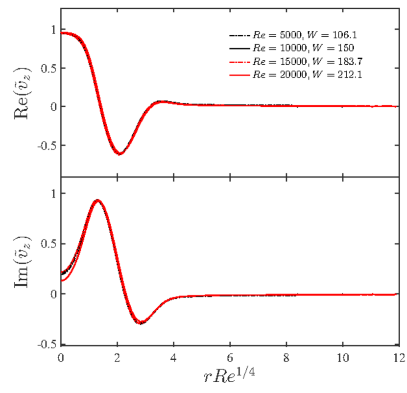
(a) $\tilde{v}_{z}$

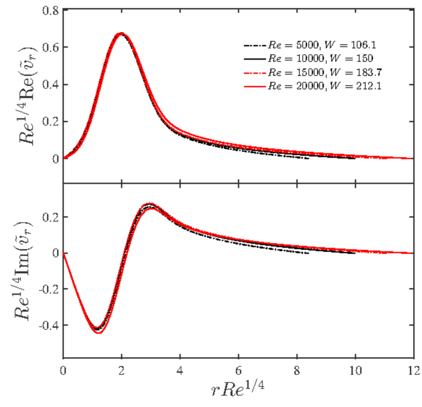
(b) $Re^{1/4}\tilde{v}_{r}$

Figure 25: Collapse of eigenfunctions at different $Re$ and $E$, but for a fixed $k=1$ for (a) axial velocity, and (b) scaled radial velocity, on scaled radial-axis in the limit $Re\rightarrow\infty$ and $W\rightarrow\infty$ for a fixed $W/Re^{1/2}$ and $\beta=0.5$, corresponding to the eigenvalues $c=0.994842+0.000112i,0.996321+0.000103i,0.996985+0.000093i$ and $0.997383+0.000085i$ respectively.

It is also possible to obtain the following scalings for a fixed $k$ by rescaling the Eqs. 13–19:

$$\delta\sim Re^{-1/4},\quad\Rey\sim E^{-2},\quad(1-c)\sim Re^{-1/2},\text{ and }\tilde{v}_{z}\sim\Rey^{1/4}\tilde{v}_{r}.$$ (34)

These scalings are illustrated by the collapse of the $\tilde{v}_{r}$ and $\tilde{v}_{z}$ eigenfunctions, corresponding to the unstable mode, as shown in Fig. 25 for a few selected pairs ($\Rey,W$) that are large enough to justify the limit $(\Rey,W)\rightarrow\infty$ such that $\Rey\sim E^{-2}$.

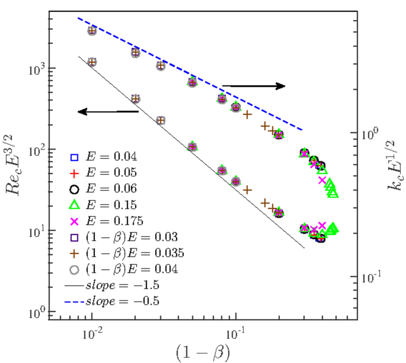
(a) $Re_{c}E^{3/2}$ and $k_{c}E^{1/2}$ vs $(1-\beta)$

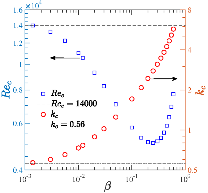
(b) $Re_{c}$, $k_{c}$ vs. $\beta$ at $E=0.01$

Figure 26: (a) Rescaled critical parameters $Re_{c}E^{3/2}$ and $k_{c}E^{1/2}$ vs. $(1-\beta)$ fall on straight lines of slopes $-3/2$ and $-1/2$, respectively, for smaller $(1-\beta)$ implying $Re_{c}\propto[(1-\beta)E]^{-3/2}$ and $k_{c}\propto[(1-\beta)E]^{-1/2}$ in the limit $\beta\rightarrow 1$. (b) Variation of critical parameters $\Rey_{c}$ and $k_{c}$ with $\beta$ for $E=0.01$.

Figure. 26(a) shows that the critical Reynolds number ($\Rey_{c}$) and critical wavenumbers ($k_{c}$) for different values of $E$ and $(1-\beta)E$ follow the scalings $\Rey_{c}\propto[(1-\beta)E]^{-3/2}$ and $k_{c}\propto[(1-\beta)E]^{-1/2}$ for $E(1-\beta)\ll 1$. We had earlier reported (Garg et al., 2018) that $Re_{c}$ diverges weakly as $\beta^{-1/4}$ for $\beta\rightarrow 0$, based on results extending down to a $\beta$ of $0.025$. However, new results for lower values of $\beta$ (down to $10^{-3}$) in Fig. 26(b) show that $Re_{c}$ does not diverge as $\beta^{-1/4}$, but appears instead to diverge more weakly, or perhaps even asymptote to a constant. Thus far, we have not found any unstable mode in the UCM limit for the corresponding $\Rey$ and $E$. However, note that the structure of the center mode changes qualitatively for the smallest $\beta$’s, characterized by the onset of small-scale oscillations (Chaudhary et al., 2019), and our efforts thus far prevent us from discriminating between $\Rey_{c}$ approaching a constant vis-a-vis a weak divergence in the said limit.

4.3 Role of stress diffusion on the unstable center mode

As discussed in the Introduction, artificial stress diffusion is often used for regularization in DNS studies of viscoelastic flows (Sureshkumar & Beris, 1995; Sureshkumar et al., 1997; Lopez et al., 2019). Recently, it has been shown that this additional diffusivity can qualitatively impact the stress dynamics (Gupta & Vincenzi, 2019), even to the extent of suppressing signatures associated with elasto-inertial turbulence (Sid et al., 2018). In this section, therefore, we briefly examine the effect of stress diffusion on the onset of the center mode instability. The constitutive equation for the polymeric stress, Eq. 2, is now augmented with the stress diffusion term:

$$W\left(\frac{\partial\boldsymbol{T}}{\partial t}+(\boldsymbol{v}\boldsymbol{.}\boldsymbol{\nabla})\boldsymbol{T}-\boldsymbol{T}\boldsymbol{.}(\boldsymbol{\nabla}\boldsymbol{v})-(\boldsymbol{\nabla}\boldsymbol{v})^{T}\boldsymbol{.}\boldsymbol{T}\right)+\boldsymbol{T}+\frac{D\lambda}{R^{2}}\nabla^{2}\boldsymbol{T}=\frac{1-\beta}{Re}\{\boldsymbol{\nabla}\boldsymbol{v}+(\boldsymbol{\nabla}\boldsymbol{v})^{T}\},$$ (35)

where $D$ is the stress diffusivity. El-Kareh & Leal (1989) showed that the stress diffusion term owes its origin to the translational diffusion of the polymer molecules and estimated the diffusivity $D$ to be $O(10^{-12})$ m²/s. Using relaxation times $\lambda\sim 10^{-3}$s reported in Chandra et al. (2018) for polymer concentrations $\sim 500$ppm, and for tube diameters $\sim 0.1$–$1$mm, the dimensionless diffusivity $D\lambda/R^{2}\sim 10^{-9}-10^{-7}$. It is useful to represent diffusive effects using a Schmidt number $Sc\equiv\nu/D=E/(D\lambda/R^{2})$, with $Sc\rightarrow\infty$ representing the absence of diffusion. The linearized equations for viscoelastic pipe flow using Eq. 35 were solved using a spectral method. Additional boundary conditions are now required for the stress components. At the pipe wall ($r=1$), the stress equation is imposed without the diffusivity, while a regularity condition for the stress is imposed at the centerline (Beris & Dimitropoulos, 1999; Lopez et al., 2019). A finite stress diffusivity regularizes the continuous spectrum modes and leads to an additional family of stable diffusive modes. The decay rate of this family increases with increasing $(D\lambda/R^{2})$. However, the discrete modes existing in the absence of stress diffusion are only weakly perturbed for small values of the diffusivity $(D\lambda/R^{2}\rightarrow 0)$.

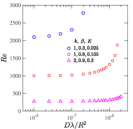
Figure 27: The effect of stress diffusion (characterized by $D\lambda/R^{2}$) on the threshold $Re$ required for onset of instability at different $E,\beta$ and $k$.

Figure 27 shows that the $Re$ for onset of the center mode instability increases with increasing ($D\lambda/R^{2}$), implying that the stress diffusivity has a stabilizing effect; for $D\lambda/R^{2}\rightarrow 0$, the onset becomes independent of the diffusivity, approaching the values shown in Fig. 27. The threshold diffusivity for stabilization is seen to depend on $E$ and $\beta$. Importantly, the instability continues to exist for the experimentally relevant values of $D\lambda/R^{2}\sim$ $10^{-9}$–$10^{-7}$, but would be suppressed at much larger values of $D\lambda/R^{2}\sim 10^{-4}$–$10^{-2}$ (or, equivalently, $Sc<1000$, for $E\sim 0.1$) used in earlier DNS studies (Sureshkumar & Beris, 1995; Sureshkumar et al., 1997; Lopez et al., 2019). Thus, consistent with the results of Sid et al. (2018), the results of Fig. 27 reinforce the importance of using simulation techniques, which avoid an artificially enhanced diffusivity, to access the axi-symmetric structures associated with the center-mode instability.

4.4 Comparison with recent experimental and DNS studies

4.4.1 Comparison with experiments

We have replotted, in Fig. 28, the results of Samanta et al. (2013) for the transition Reynolds number $\Rey_{t}$ as a function of $E(1-\beta)$, based on the reported viscosities and relaxation times of the different polymer solutions used in the experiments. The present theoretical results yield similar critical Reynolds numbers $\Rey_{c}$ only at much higher values of $E(1-\beta)$. Samanta et al. (2013) estimated the relaxation time using the CaBER technique (Anna & McKinley, 2001), in which the flow is extensional, and the polymer chains are highly stretched. However, the CaBER procedure is known to have some disadvantages in the estimation of relaxation time for polymers in low-viscosity solvents due to the neglect of inertia in the filament thinning dynamics. The CaBER relaxation time also exhibits a significant concentration dependence even below the nominal overlap concentration (Clasen et al., 2006). The data for $\Rey_{t}$ from the experiments of Chandra et al. (2018), also plotted in Fig. 28, shows good agreement with the theoretical $Re_{c}$’s; in that, both threshold $Re$’s are of the same order of magnitude for comparable $E(1-\beta)$. Chandra et al. (2018) used small-amplitude oscillatory strain experiments to infer the relaxation times; in contrast to CaBER, the polymer chains are not greatly perturbed about their equilibrium conformations. While the threshold $Re$’s from Chandra et al. (2018) are comparable to theory, the latter predicts $\Rey_{c}\sim E^{-3/2}$ along the lower branch of the theoretical envelope, and $\Rey_{t}\sim E^{-1/2}$ in Chandra et al. (2018). This difference in the scaling exponents could be due to shear thinning in the experiments, which can also significantly alter the parabolic nature of the base velocity profile. These effects are not accounted for in the Oldroyd-B model used in this study. The following scaling analysis examines the role of shear thinning on the scaling exponent characterizing the $Re_{c}$ vs. $E$ behaviour for small $E$. We begin by noting the limiting behaviour of viscosity and relaxation time, for large $W$, for the more realistic FENE-P model, where shear thinning arises on account of the chains being finitely extensible (Bird et al., 1980):

$$\eta_{1}\sim\eta(\dot{\gamma}\lambda)^{-2/3},\quad\text{and }\lambda_{1}=\lambda(\dot{\gamma}\lambda)^{-4/3},$$ (36)

where $\eta$ and $\lambda$ are viscosity and relaxation time at zero shear rate ($\dot{\gamma}=U/R$). The effective Reynolds number $\Rey_{1}$ and Weissenberg number $W_{1}$, evaluated using the shear-rate dependent viscosity and relaxation time, are given in terms of those involving the corresponding zero-shear-rate quantities, as

$$\Rey_{1}=\frac{\rho UR}{\eta_{1}}=E^{2/3}\Rey^{5/3},\text{ and }W_{1}=\frac{\lambda_{1}U}{R},$$ (37)

and the effective elasticity number $E_{1}$ becomes

$$E_{1}=\frac{W_{1}}{\Rey_{1}}=\frac{\lambda_{1}\eta_{1}}{\rho R^{2}}=E^{-1}\Rey^{-2}\,.$$ (38)

We now postulate that the scaling for $\Rey_{c}$ determined above for an Oldroyd-B fluid, is valid for a FENE-P fluid as well, but with $Re_{1}$ and $E_{1}$ replacing $Re$ and $E$ in order to account for the shear-rate dependence of viscosity and relaxation time. Using Eqs. 37–38 in the theoretical scaling $\Rey_{1,c}\propto E_{1}^{-3/2}$ gives $\Rey_{c}\propto E^{-5/8}$; the scaling exponent now being closer to that ($-1/2$) observed in experiments (Chandra et al., 2018, 2020). A similar argument has been used earlier to successfully account the effect of shear thinning on the onset of inertialess elastic instability in Taylor-Couette flow (Larson et al., 1994).

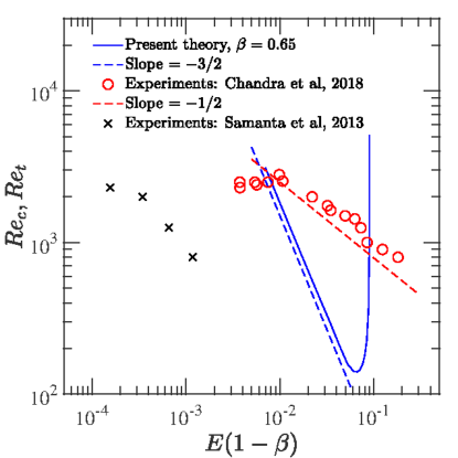
Figure 28: Comparison of the present theoretical predictions with experimental results of Samanta et al. (2013) and Chandra et al. (2018).

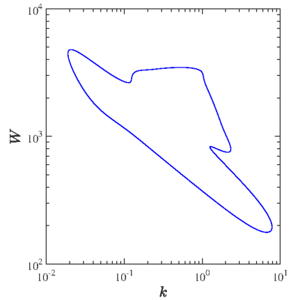
Figure 29: Neutral stability curve in the $W$–$k$ plane at fixed $\Rey=3500$ and $\beta=0.9$; the region inside the loop is unstable.

4.4.2 Comparison with DNS of Lopez et al. (2019)

The recent DNS study by Lopez et al. (2019) on viscoelastic pipe flow used the FENE-P model and showed that at a fixed $\Rey=3500$, the flow fully relaminarizes as $W$ is increased, and at even larger $W$, the laminar state again becomes unstable, with the post-instability friction factor approaching the MDR asymptote. It is worth noting that complete relaminarization was possible because of domains longer than those considered by Graham and co-workers who had observed the so-called hibernating state in the shorter domains (Xi & Graham, 2010, 2012; Graham, 2014; Xi, 2019). In Fig. 29, we show the neutral stability curve in the $W$–$k$ plane corresponding to the center mode instability for $\Rey=3500$ and $\beta=0.9$ (parameters corresponding to the DNS of Lopez et al. (2019)), according to which the flow is unstable in the range $176.9<W<4783.6$. The closed loop in the $W$–$k$ plane, at a fixed $\Rey=3500$, arises because the center mode instability is absent both in the low- and high-$W$ limits, as can be inferred from the corresponding neutral curves in the $\Rey$–$k$ plane shown in Fig. 18(b). The range of $W$ corresponding to the $W$-$k$ loop where the linear instability of the center mode is found is significantly higher than the range ($16<W<80$) over which EIT was observed in the simulations of Lopez et al. (2019). However, the Oldroyd-B model used here does not account for shear thinning effects inherent in the FENE-P model used in their simulations. More work is thus needed to address these discrepancies between the theoretical predictions and experimental and/or DNS studies.

5 Conclusion and Outlook

The present work builds on our earlier effort (Garg et al., 2018) to provide the first comprehensive set of results from a linear stability analysis of viscoelastic pipe flow using the Oldroyd-B model. Contrary to the prevailing view, and in direct contrast to its Newtonian counterpart, pipe flow of an Oldroyd-B fluid is unstable to infinitesimal perturbations. The unstable eigenfunction is a center mode with phase speed close to the maximum of the base-state flow. We provide a detailed description of the emergence and nature of the unstable center mode, and its relation to the continuous spectra in the linearized spectrum. Crucially, despite the phase speed being close to unity (the rationale behind the ‘center mode’ terminology), the eigenfunctions for the unstable mode are not localized near the centerline in most of the parameter space, especially the region accessible to experiments. A bit surprisingly, perhaps, the flow appears to be stable in the limit of an upper-convected Maxwell fluid, implying that the destabilizing mechanism involves a subtle interplay of fluid inertia, elasticity and solvent viscous effects. In the asymptotic limit corresponding to dilute polymer solutions ($(1-\beta)\ll 1$ and $E(1-\beta)\ll 1$), consistent with scaling arguments, the numerical results show that the critical Reynolds number scales as $Re_{c}\sim(E(1-\beta))^{-3/2}$, while the critical wavenumber scales as $k_{c}\sim(E(1-\beta))^{-1/2}$. The radial lengthscale is now comparable to $k_{c}^{-1}$, so that the unstable eigenfunction in this limit does become confined to a thin region in the vicinity of the pipe centerline.

For $E$ and $\beta$ pertaining to the experiments of Samanta et al. (2013) with polymer concentrations greater than $300$ppm, where the authors did observe the transition to be supercritical, results from our linear stability theory yield much higher transition $Re$’s than the experiments. Equivalently, our results do predict a threshold $Re$ of $O(800)$, the one observed for the $500$ ppm solution in Samanta et al. (2013), but only at much higher $E$’s. This discrepancy could perhaps be attributed to artifacts related to the CaBER procedure used by Samanta et al. (2013) to characterize the relaxation time. This procedure is known to lead to a spurious underestimation of the relaxation time (recall that the elasticity number $E$ is proportional to the polymer relaxation time) for solutions well below the nominal overlap concentration; there might be additional problems arising from use of low viscosity fluids (Clasen et al., 2006). However, our theoretical predictions are broadly consistent with the observations of Chandra et al. (2018), who used small-amplitude oscillatory strain experiments to infer the relaxation time, wherein the polymer chains are not greatly perturbed about their equilibrium conformations. In their rheological characterization, the solvent viscosity was significantly enhanced to enable a measurable signal, while maintaining a fixed concentration in the dilute regime (unlike CaBER). For the range of $E$ and $\beta$ corresponding to the latter experiments, linear stability theory predicts $Re_{c}\sim 10^{2}$–$10^{3}$, while experiments report $Re_{t}\sim 800-1000$. However, observations seem to satisfy the scaling relation $Re_{t}\sim(E(1-\beta))^{-1/2}$ in contrast to the $-3/2$ exponent predicted by our theory (see Fig. 23(a)). One aspect that could be relevant in experiments, but not accounted for in the Oldroyd-B model, is shear thinning. Based on a scaling analysis for the FENE-P model that incorporated the asymptotic behavior of the relaxation time, and the resulting shear thinning, for large $W$, the aforementioned scaling exponent changes from $-3/2$ to $-5/8$, the latter being closer to the experimental exponent of $-1/2$. Nevertheless, more work is needed to reconcile theoretical predictions and observations, in terms of accurate characterization of the polymer relaxation time (in the dilute regime), a careful detection of the onset of transition by multiple means (such as PIV and pressure-drop measurements), and by using realistic constitutive models (in the stability analysis) that extend across the overlap concentration, accounting for dynamics in both the dilute and semi-dilute regimes (Prabhakar et al., 2016).

Prior to the present work, the prevailing understanding of stability of viscoelastic flows and turbulent drag reduction was predicated on an elastic modification of the Newtonian transition scenario. The latter is known to be subcritical, wherein the actual transition is believed to be preceded by the appearance of (nonlinear) three-dimensional, exact coherent states (ECS). As $\Rey$ is increased, the laminar basin of attraction shrinks, with the concomitant appearance of more unstable ECS’s. The turbulent trajectory is proposed to sample the phase space of such solutions in a chaotic manner (Budanur et al., 2017); a sustained turbulent state, beyond a finite threshold $Re$, requires spatial-temporal dynamics that includes merging of localized ECS solutions (Avila et al., 2011; Chantry et al., 2014; Barkley, 2016). The work of Graham and co-workers (Stone et al., 2002; Stone & Graham, 2003; Stone et al., 2004; Li & Graham, 2007; Graham, 2014) explored in detail the effect of viscoelasticity on the above scenario. Specifically, Li & Graham (2007) have shown that viscoelasticity suppresses the appearance of the relatively simple (travelling waves) ECS in channel flow. An extrapolation, entailing an assumption that viscoelasticity has a similar effect on the other ECS’s, with a non-trivial time dependence, implies that the onset of the sub-critical transition is delayed by viscoelasticity. As mentioned earlier in Sec.1.3, this conclusion has some indirect experimental support (Samanta et al., 2013; Chandra et al., 2018). However, the transition scenario at higher $E$’s (equivalent to higher polymer concentrations), apart from being at lower $Re$’s, appears to have a fundamentally different character, being independent of external perturbations. Our analysis, consistent with these observations, shows that pipe flow is unstable to infinitesimal disturbances at sufficiently high $E$. Results from recent computations (Sid et al., 2018) emphasize the importance of 2D (span-wise oriented) structures in the elasto-inertial turbulent state for channel flow, in marked contrast to the 3D Newtonian scenario, reinforcing the notion of an underlying instability to axisymmetric perturbations examined here. Importantly, the nature of the elasto-inertial coherent structures identified in DNS studies of both viscoelastic channel and pipe-flow (Sid et al., 2018; Lopez et al., 2019) are quite similar, pointing to a generic mechanism operative in both these geometries, again consistent with our own finding of an analogous center mode instability in channel flow (Garg et al., 2018; Khalid et al., 2020).

Our study is a clear call for a reassessment of the current understanding of turbulent drag reduction by polymers, in particular, of the nature of the maximum-drag-reduced (MDR) regime and its relation to both the laminar and (Newtonian) turbulent states. Recent experimental results of Choueiri et al. (2018) explicitly demonstrate the link between elasto-inertial turbulence and the maximum-drag-reduction (MDR) regime, by showing that the same physical mechanisms underlie the two states (at least for the moderate $Re$’s accessed in the experiments). Both experiments and DNS studies (Choueiri et al., 2018; Shekar et al., 2019; Lopez et al., 2019) have also shown that MDR can also be reached via a direct pathway from the laminar state of a polymer solution, without entering the Newtonian turbulent regime. Thus, the terminology of ‘drag reduction’ is somewhat ambiguous: the MDR state was traditionally viewed as a drag-reduced state from Newtonian turbulence upon addition of polymers. Based on the above picture, and the linear instability identified in this work, we conjecture that the aforementioned direct pathway to MDR could be achieved via a nonlinear saturation of the elasto-inertial center mode instability of viscoelastic pipe flow, with a concomitant mild drag enhancement relative to the laminar state. The eigenfunctions corresponding to the unstable mode identified in this study should form a template for future nonlinear studies aimed at identifying novel nonlinear elasto-inertial structures that might play an important role in understanding the nature of the MDR state at large elasticity numbers. As a first step in this direction, results from a weakly-nonlinear analysis (along the lines of Stuart, 1960; Watson, 1960), which are largely consistent with the conclusions of the linear stability analysis presented here, will be reported in a future communication.

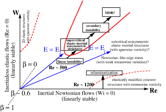
Figure 30: A schematic representation of various transition scenarios in viscoelastic pipe flow in the $\Rey$–$W$ (for a fixed $\beta$) plane. The boundaries shown using dotted red lines represent subcritical bifurcations, while the unstable boundary due to the center mode instability is shown using a continuous red line. The oblique blue lines indicate experimental paths in which flow rate is increased (in a pipe of a given diameter and for a given polymer solution) with $E=W/Re$ being constant; $E_{2}>E_{1}$.

Based on the above discussion, it is useful to organize our understanding of the various possible transition scenarios in viscoelastic pipe flows in the form of a ‘phase diagram’ in $\Rey$–$W$ (and $\beta$) space. This is shown as a schematic in Fig. 30 for a fixed $\beta\sim 0.5$ and higher; for $\beta\rightarrow 0$, $Re_{c}\sim O(10^{4})$ (see Fig. 26(b)), and it is not clear if the linear instability (at such high $Re$) would continue to be practically relevant. Note that an experimental pathway representing an increase in flow rate (for a given pipe diameter and polymer solution) will appear as an oblique line (with slope $E=W/Re$) in the $Re$-$W$ plane (Graham, 2014; Xi, 2019). It helps to consider two limiting sequences in this plane. The first corresponds to increasing $Re$ at $W=0$ - the Newtonian transition. The sub-critical nature of this transition and the underlying role of the ECS’s is now relatively well established. The effect of viscoelasticity on this picture has been discussed in the earlier paragraph, the main idea being that the suppression of the ECS’s by elasticity, at $Re$’s greater than the Newtonian threshold ($Re\sim 2000$), has been interpreted as the reason for a delayed transition; the regime of existence of the ECS’s for $W=0$, and the postponement of this regime with increasing $W$ is marked with a dashed red line near the $Re$-axis in Fig. 30. It is worth noting that despite the sharp contrast in the linear (modal) eigenfunctions for pipe and channel flow (the absence of the TS wall mode in pipe flow being an example), the Newtonian ECS’s have a similar character across all of the canonical shearing flows, consisting of counter-rotating vortices and stream-wise streaks in all cases. Thus, the extrapolation of the effects of viscoelasticity to the pipe geometry, based on the domain of existence of finite-$W$ ECS’s in the channel geometry, is reasonable. Nevertheless, there is a need to examine the nature of elastically-modified pipe flow ECS’s, as a function of $W$, in order to render the arguments quantitative. As already indicated above, such ECS-based arguments are no longer valid at higher $E$ when the ECS’s are absent.

The understanding of the MDR regime attained at higher $E$’s (or higher $W$’s with $Re$ fixed), shown schematically by the path $E_{1}$ in Fig. 30, was until recently based on a series of minimal (channel) flow unit simulations carried out by Graham and co-workers (Xi & Graham, 2010, 2012; Graham, 2014; Xi, 2019). The hypothesis advanced was that of the dynamics in the MDR state corresponding to that of a largely unaltered Newtonian ‘edge state’, a marginal state whose stable manifold forms the boundary separating the laminar fixed point and the turbulent attractor. This edge state manifests as prolonged periods of so-called hibernating turbulence, characterized by subdued fluctuatons and an associated weak stream-wise variation. The primarily Newtonian character of this edge-state was proposed as an explanation for the independence of the MDR regime with respect to polymer characteristics. In effect, the originally unstable Newtonian edge state is apparently stabilized at higher $E$’s. The connection between the disappearance of the ECS’s in earlier work by Graham’s group, and the subsequent appearance of a stabilized edge state at higher $E$’s, has not been clarified from a dynamical systems view point in terms of an appropriate viscoelastic state space (it is worth noting that, for the Newtonian case, most of the lower-branch travelling-wave solutions are known to lie on the aforementioned laminar-turbulent boundary, and are therefore edge states, albeit unstable). Importantly, however, the veracity of the above edge-state-based interpretation has been recently challenged by simulations in longer domains (Lopez et al., 2019) where the hibernating state is found to give way to spatio-temporal intermittency, and subsequent relaminarization.

At sufficiently high $E$’s (shown schematically by the path $E_{2}$ in Fig. 30), there is the possibility of the center-mode instability (region in Fig. 30 demarcated by a continuous red curve) leading to a direct pathway from the laminar state to a non-linear state characterized by essentially axisymmetric elasto-inertial structures that presumably arise from a saturation of the growing center mode. These structures might then form the backbone of EIT dynamics. The identification of this pathway confirms the speculation of a linear instability at high $E$ (see Fig. 4 of Graham, 2014), thereby augmenting the various possible transition scenarios in the $Re$-$W$ plane. Based on the $E$-intervals identified here, for the center-mode instability, there does appear to be a region in the $Re$-$W$ plane where the elastically modified ECS’s are absent and pipe flow is still linearly stable. In this regime, one might either expect dynamics corresponding to the Newtonian edge state, proposed by Graham and coworkers (described above), or an entirely new set of subcritical elasto-inertial structures. In the latter regard, it is tempting to postulate the 2D, nonlinear mechanism of Shekar et al. (2019), with signatures similar to the least stable Newtonian TS mode, to play a role. In contrast to the qualitative similarities in the nature of Newtonian pipe and channel ECS’s, however, and as pointed out in Sec. 3.3, differences in the axisymmetric pipe and two-dimensional channel flow viscoelastic spectra render this wall-mode based mechanism untenable for pipe flow. This is because the center mode in Newtonian pipe flow, while being stable, still has a decay rate smaller than that of the wall mode. Further, there is a significant regime in the $Re$–$W$ plane where the continuous spectra are the least stable. Thus, unlike the proposal of Shekar et al. (2019) for channel flow, a novel sub-critical elasto-inertial dynamics, in pipe flow, would seem to have to account for the dynamics of the continuous spectrum at leading order (Balmforth et al., 2013). Further, any additional dynamics related to the discrete modes would still appear to be dominated by the center mode on account of its lower decay rate. Based on this qualitative picture, we have indicated (in Fig. 30) the two possible mechanisms in the region that separates the regimes corresponding to the center-mode instability, and the subcritical ECS. Note that any pathway leading upto the EIT regime, at a fixed $Re$, involves a transition from coherent structures with stream-wise vorticity to those with span-wise vorticity.

Finally, at the highest $E$’s, one approaches the second limiting sequence in Fig. 30, which is that of increasing $W$ at $Re=0$, and therefore, concerns the inertia-less transition to elastic turbulence (Groisman & Steinberg, 2000), which is believed to follow the traditional nonlinear route (Stuart, 1960; Watson, 1960). van Saarloos and co-workers (Meulenbroek et al., 2003, 2004; Morozov & van Saarloos, 2005, 2007), based on a viscoelastic analogue of the original Stuart-Landau expansion, have shown that inertia-less pipe flow undergoes a sub-critical bifurcation to a nonlinear two-dimensional state (represented using a dotted red line near $Re=0$ in Fig. 30); the same is true for plane Couette and Poiseuille flows. This scenario has found some support in experiments (Pan et al., 2013). These weakly nonlinear analyses are based on the existence of an unstable/weakly stable discrete mode well separated from the remainder of the spectrum. This is indeed true for inertia-less viscoelastic flows where the spectrum consists of a small number of discrete modes (Renardy & Renardy, 1986; Wilson et al., 1999), in addition to the continuous spectra. However, the spectrum becomes far more complicated with increasing $Re$, with there being no clear separation in the above sense (see Fig. 12(a) and those in Chaudhary et al., 2019). In fact, for moderate $Re$ and for small but finite $E$, as pointed out above, there exist scenarios wherein no discrete modes are present above the continuous spectrum (e.g., for $E<0.6$ and $Re=500$, $\beta=0.96$ in Fig. 5(a)), thereby necessitating the consideration of the CS at leading order in the nonlinear analysis. Clearly, therefore, the nonlinear mechanisms proposed by van Saarloos and co-workers are restricted to modest $Re$, and cannot serve as an explanation for transition to EIT.

In summary, our finding of a linear instability in viscoelastic pipe flow marks a possible paradigm shift from both classical and modern theoretical work on Newtonian fluids, by providing a natural explanation for the connection between the laminar state and the elasto-inertial state underlying the so-called maximum-drag-reduced regime.

Equal contribution of authorship

I. C and P. G contributed equally to this work.

Declaration of interests

The authors report no conflict of interest.

References

- Anna & McKinley (2001) Anna, Shelley L. & McKinley, Gareth H. 2001 Elasto-capillary thinning and breakup of model elastic liquids. Journal of Rheology 45 (1), 115–138.
- Avila et al. (2011) Avila, K., Moxey, D., Lozar, A. De, Barkley, D. & Hof, B. 2011 The onset of turbulence in pipe flow. Science 333, 192–196.
- Balmforth et al. (2013) Balmforth, N. J., Morrison, P. J. & Thiffeault, J. L. 2013 Pattern formation in Hamiltonian systems with continuous spectra; a normal-form single-wave model, arXiv: 1303.0065.
- Barkley (2016) Barkley, D. 2016 Theoretical perspective on the route to turbulence in a pipe. J. Fluid Mech. 803.
- Batchelor & Gill (1962) Batchelor, G. K. & Gill, A. E. 1962 Analysis of the stability of axisymmetric jets. J. Fluid Mech. 14, 529–551.
- Beris & Dimitropoulos (1999) Beris, A. N. & Dimitropoulos, C. D 1999 Pseudospectral simulation of turbulent viscoelastic channel flow. Comp. Meth. Appl. Mech. Eng. 180, 365–392.
- Bertola et al. (2003) Bertola, V., Meulenbroek, B., Wagner, C., Storm, C., Morozov, A., van Saarloos, W. & Bonn, D. 2003 Experimental evidence for an intrinsic route to polymer melt fracture phenomena: A nonlinear instability of viscoelastic Poiseuille flow. Phys. Rev. Lett. 90 (11), 114502.
- Bird et al. (1980) Bird, R.B., Dotson, P.J. & Johnson, N.L. 1980 Polymer solution rheology based on a finitely extensible bead—spring chain model. J. non-Newtonian Fluid Mech. 7, 213–235.
- Bird et al. (1977) Bird, R. B., Armstrong, R. C. & Hassager, O. 1977 Dynamics of Polymeric liquids, Vol 1 Fluid Mechanics. New York: John Wiley.
- Boger & Nguyen (1978) Boger, D. V. & Nguyen, H. 1978 A model viscoelastic fluid. Polymer Engineering and Science 18, 1037–1043.
- Boyd (2000) Boyd, J. P. 2000 Chebyshev and Fourier Spectral Methods. Dover Publications.
- Budanur et al. (2017) Budanur, N. B., Short, K. Y., Farazmand, M., Willis, A. P. & Cvitanović, P. 2017 Relative periodic orbits form the backbone of turbulent pipe flow. J. Fluid Mech. 833, 274–301.
- Butler & Farrell (1992) Butler, K. M. & Farrell, B. F. 1992 Three-dimensional optimal perturbations in viscous shear flows. Phys. Fluids A 4, 1637.
- Castro & Squire (1968) Castro, W. & Squire, W. 1968 The effect of polymer additives on transition in pipe flow. Applied Scientific Research 18, 81–96.
- Chandra et al. (2018) Chandra, B., Shankar, V. & Das, D. 2018 Onset of transition in the flow of polymer solutions through microtubes. J. Fluid Mech. 844, 1052––1083.
- Chandra et al. (2020) Chandra, B., Shankar, V. & Das, D. 2020 Early transition, relaminarization and drag reduction in the flow of polymer solutions through microtubes. J. Fluid Mech. 885, A47.
- Chantry et al. (2014) Chantry, M., Willis, A. P. & Kerswell, R. R. 2014 Genesis of streamwise-localized solutions from globally periodic traveling waves in pipe flow. Phys. Rev. Lett. 112, 164501.
- Chaudhary et al. (2019) Chaudhary, I., Garg, P., Shankar, V. & Subramanian, G. 2019 Elasto-inertial wall-mode instabilities in viscoelastic channel flows. J. Fluid Mech. 881, 119–163.
- Chaudhary et al. (2020) Chaudhary, I., Shankar, V. & Subramanian, G. 2020 Stability of viscoelastic pipe flow in the limit of infinite reynolds and weissenberg numbers. In Preparation.
- Chokshi & Kumaran (2009) Chokshi, P. & Kumaran, V. 2009 Stability of the plane shear flow of dilute polymeric solutions. Phys. Fluids 21, 014109.
- Choueiri et al. (2018) Choueiri, G. H., Lopez, J. M. & Hof, B. J. 2018 Exceeding the asymptotic limit of polymer drag reduction. Phys. Rev. Lett. 120 (12), 124501.
- Clasen et al. (2006) Clasen, C., Plog, J. P., Kulicke, W.-M., Owens, M., Macosko, C., Scriven, L. E., Verani, M. & McKinley, G. H. 2006 How dilute are dilute solutions in extensional flows? J. Rheol. 50 (6), 849–881, arXiv: https://doi.org/10.1122/1.2357595.
- Clever & Busse (1992) Clever, R. M. & Busse, F. H. 1992 Three-dimensional convection in a horizontal fluid layer subjected to a constant shear. J. Fluid Mech. 234, 511–527.
- Corcos & Sellars (1959) Corcos, G. M. & Sellars, J. R. 1959 On the stability of fully developed pipe flow. J. Fluid Mech. 5, 97–112.
- De Angelis et al. (2002) De Angelis, E., Casciola, C. M. & R., Piva. 2002 DNS of wall turbulence: dilute polymers and self-sustaining mechanisms. Comp. Fluids 31, 495–507.
- Draad et al. (1998) Draad, A. A., Kuiken, G. D. C. & Nieuwstadt, F. T. M. 1998 Laminar–turbulent transition in pipe flow for Newtonian and non-Newtonian fluids. J. Fluid Mech. 377, 267–312.
- Drazin & Reid (1981) Drazin, P. G. & Reid, W. H. 1981 Hydrodynamic Stability. Cambridge University Press.
- Dubief et al. (2013) Dubief, Y., Terrapon, V. E. & Soria, J. 2013 On the mechanism of elasto-inertial turbulence. Phys. Fluids 25 (11), 110817.
- Dubief et al. (2004) Dubief, Y., White, C. M., Terrapon, V. E., Shaqfeh, E. S. G., Moin, P. & Lele, S. K. 2004 On the coherent drag-reducing and turbulence-enhancing behaviour of polymers in wall flows. J. Fluid Mech. 514, 271–280.
- Eckhardt et al. (2007) Eckhardt, B., Schneider, T. M., Hof, B. & Westerweel, J. 2007 Turbulence transition in pipe flow. Annu. Rev. Fluid Mech. 39, 447–468.
- El-Kareh & Leal (1989) El-Kareh, Ardith W & Leal, L Gary 1989 Existence of solutions for all Deborah numbers for a non-Newtonian model modified to include diffusion. J. Non-Newtonian Fluid Mech. 33, 257–287.
- Forame et al. (1972) Forame, P. C., Hansen, R. J. & Little, R. C. 1972 Observations of early turbulence in the pipe flow of drag reducing polymer solutions. AIChE Journal 18 (1), 213–217.
- Garg et al. (2018) Garg, P., Chaudhary, I., Khalid, M., Shankar, V & Subramanian, G. 2018 Viscoelastic pipe flow is linearly unstable. Phys. Rev. Lett. 121, 024502.
- Garg & Rouleau (1972) Garg, VK & Rouleau, WT 1972 Linear spatial stability of pipe Poiseuille flow. J. Fluid Mech. 54, 113–127.
- Giles (1967) Giles, W. B.; Pettit, W. T. 1967 Stability of dilute viscoelastic flows. Nature 216.
- Gill (1965a) Gill, A. E. 1965a A mechanism for instability of plane Couette flow and of Poiseuille flow in a pipe. J. Fluid Mech. 21, 503–511.
- Gill (1965b) Gill, A. E. 1965b On the behaviour of small disturbances to Poiseuille flow in a circular pipe. J. Fluid Mech. 21, 145–172.
- Goldstein et al. (1969) Goldstein, R. J., Adrian, R. J. & Kreid, D. K. 1969 Turbulent and transition pipe flow of dilute aqueous polymer solutions. Industrial & Engineering Chemistry Fundamentals 8 (3), 498–502.
- Gorodtsov & Leonov (1967) Gorodtsov, V. A. & Leonov, A. I. 1967 On a linear instability of a plane parallel Couette flow of viscoelastic fluid. J. Appl. Maths Mech. 31, 310–319.
- Graham (1998) Graham, M. D. 1998 Effect of axial flow on viscoelastic Taylor-Couette instability. J. Fluid Mech. 360, 341–374.
- Graham (2014) Graham, M. D. 2014 Drag reduction and the dynamics of turbulence in simple and complex fluids. Phys. Fluids 26, 101301.
- Grillet et al. (2002) Grillet, A. M., Bogaerds, A. C. B., Peters, G. W. M. & Baaijens, F. P. T. 2002 Stability analysis of constitutive equations for polymer melts in viscometric flows. J. Non-Newtonian Fluid Mech. 103, 221–250.
- Groisman & Steinberg (2000) Groisman, A. & Steinberg, V. 2000 Elastic turbulence in a polymer solution flow. Nature 405, 53–55.
- Grossmann (2000) Grossmann, S. 2000 The onset of shear flow turbulence. Rev. Mod. Phys. 72, 603.
- Gupta & Vincenzi (2019) Gupta, A. & Vincenzi, D. 2019 Effect of polymer-stress diffusion in the numerical simulation of elastic turbulence. J. Fluid Mech. 870, 405–418.
- Hansen (1973) Hansen, R. J. 1973 Stability of laminar pipe flows of drag reducing polymer solutions in the presence of high-phase-velocity disturbances. AIChE J. 19, 298–304.
- Hansen et al. (1973) Hansen, R. J., Little, R. & Forame, P. G. 1973 Experimental and theoretical studies of early turbulence. Journal of Chemical Engineering of Japan 6 (4), 310–314.
- Hansen & Little (1974) Hansen, R. J. & Little, R. C. 1974 Early turbulence and drag reduction phenomena in larger pipes. Nature 252, 690.
- Ho & Denn (1977) Ho, T. C. & Denn, M. M. 1977 Stability of plane Poiseuille flow of a highly elastic liquid. J. Non-Newtonian Fluid Mech. 3 (2), 179 – 195.
- Hoyt (1977) Hoyt, J. W. 1977 Laminar-turbulent transition in polymer solutions. Nature 270, 508.
- Jones et al. (1976) Jones, W. M., Marshall, D. E. & Walker, P. C. 1976 The flow of dilute aqueous solutions of macromolecules in various geometries. ii. straight pipes of circular cross-section. Journal of Physics D: Applied Physics 9 (5), 735.
- Kaffel & Renardy (2010) Kaffel, A. & Renardy, M. 2010 On the stability of plane parallel viscoelastic shear flows in the limit of infinite Weissenberg and Reynolds numbers. J. Non-Newtonian Fluid Mech. 165, 1670–1676.
- Kerswell (2018) Kerswell, R. 2018 Nonlinear nonmodal stability theory. Ann. Rev. Fluid Mech. 50, 319–345.
- Kerswell (2005) Kerswell, R. R. 2005 Recent progress in understanding the transition to turbulence in a pipe. Nonlinearity 18 (6), R17.
- Khalid et al. (2020) Khalid, M., Chaudhary, I., Garg, P., Shankar, V. & Subramanian, G. 2020 Elasto-inertial center-mode instabilities in plane channel flow of an Oldroyd-B fluid. In Preparation.
- Khorrami et al. (1989) Khorrami, M. R., Malik, M. R. & Ash, R. L. 1989 Application of spectral collocation techniques to the stability of swirling flows. Journal of Computational Physics 81, 206–229.
- Kumar & Shankar (2005) Kumar, A. S. & Shankar, V. 2005 Instability of high-frequency modes in viscoelastic plane Couette flow past a deformable wall at low and finite Reynolds number. J. Non-Newtonian Fluid Mech. 125, 121–141.
- Larson et al. (1994) Larson, R.G., Muller, S.J. & Shaqfeh, E.S.G. 1994 The effect of fluid rheology on the elastic Taylor-Couette instability. J. non-Newtonian Fluid Mech. 51, 195–225.
- Larson (1988) Larson, R. G. 1988 Constitutive Equations for Polymer Melts and Solutions. Butterworths.
- Larson (1992) Larson, R. G. 1992 Instabilities in viscoelastic flows. Rheologica Acta 31, 213–263.
- Larson et al. (1990) Larson, R. G., Shaqfeh, E. S. G. & Muller, S. J. 1990 A purely elastic instability in Taylor-Couette flow. J. Fluid Mech. 218, 573–600.
- Lee & Finlayson (1986) Lee, K. C. & Finlayson, B. A. 1986 Stability of plane Poiseuille and Couette flow of a Maxwell fluid. J. Non-Newtonian Fluid Mech. 21, 65–78.
- Li & Graham (2007) Li, W. & Graham, M. D. 2007 Polymer induced drag reduction in exact coherent structures of plane Poiseuille flow. Phys. Fluids 19, 083101.
- Li et al. (2006) Li, W., Xi, L. & Graham, M. D. 2006 Nonlinear travelling waves as a framework for understanding turbulent drag reduction. J. Fluid Mech. 565, 353–362.
- Li et al. (2012) Li, X.-B., Li, F.-C., Cai, W.-H., Zhang, H.-N. & Yang, J.-C. 2012 Very-low-re chaotic motions of viscoelastic fluid and its unique applications in microfluidic devices: A review. Experimental Thermal and Fluid Science 39, 1 – 16.
- Lopez et al. (2019) Lopez, J. M., Choueiri, G. H. & Hof, B. 2019 Dynamics of viscoelastic pipe flow at low reynolds numbers in the maximum drag reduction limit. J. Fluid Mech. 874, 699–719.
- Mack (1976) Mack, L. M. 1976 A numerical study of the temporal eigenvalue spectrum of the Blasius boundary layer. J. Fluid Mech. 73, 497–520.
- Meseguer & Trefethen (2003) Meseguer, A. & Trefethen, L. N. 2003 Linearized pipe flow to Reynolds number . J. Comp. Phys. 186, 178–197.
- Meulenbroek et al. (2003) Meulenbroek, B., Storm, C., Bertola, V., Wagner, C., Bonn, D. & van Saarloos, W. 2003 Intrinsic route to melt fracture in polymer extrusion: A weakly nonlinear subcritical instability of viscoelastic Poiseuille flow. Phys. Rev. Lett. 90, 024502.
- Meulenbroek et al. (2004) Meulenbroek, B., Storm, C., Morozov, A. N. & van Saarloos, W. 2004 Weakly nonlinear subcritical instability of viscoelastic Poiseuille flow. J. Non-Newtonian Fluid Mech. 116, 235–268.
- Morozov & van Saarloos (2005) Morozov, A. N. & van Saarloos, W. 2005 Subcritical finite-amplitude solutions for plane Couette flow of viscoelastic fluids. Phys. Rev. Lett. 95, 024501.
- Morozov & van Saarloos (2007) Morozov, A. N. & van Saarloos, W. 2007 An introductory essay on subcritical instabilities and the transition to turbulence in visco-elastic parallel shear flows. Physics Reports 447, 112–143, Non-equilibrium physics: From complex fluids to biological systems I. Instabilities and pattern formation.
- Mullin (2011) Mullin, T. 2011 Experimental studies of transition to turbulence in a pipe. Ann. Rev. Fluid Mech. 43, 1–24.
- Nagata (1990) Nagata, M. 1990 Three-dimensional finite-amplitude solutions in plane Couette flow: bifurcation from infinity. J. Fluid Mech. 217, 519–527.
- Pakdel & McKinley (1996) Pakdel, P. & McKinley, G. H. 1996 Elastic instability and curved streamlines. Phys. Rev. Lett. 77, 2459.
- Pan et al. (2013) Pan, L., Morozov, A., Wagner, C. & Arratia, P. E. 2013 Nonlinear elastic instability in channel flows at low Reynolds numbers. Phys. Rev. Lett. 110, 174502.
- Pfenniger (1961) Pfenniger, W. 1961 Transition in the inlet length of tubes at high Reynolds numbers. In Boundary layer and flow control (ed. G. V. Lachman), pp. 970–980. Pergamon, New York.
- Prabhakar et al. (2016) Prabhakar, R., Gadkari, S., Gopesh, T. & Shaw, M. J. 2016 Influence of stretching induced self-concentration and self-dilution on coil-stretch hysteresis and capillary thinning of unentangled polymer solutions. Journal of Rheology 60 (3), 345–366.
- Pringle & Kerswell (2010) Pringle, C. C. T. & Kerswell, R. R. 2010 Using nonlinear transient growth to construct the minimal seed for shear flow turbulence. Phys. Rev. Lett. 105, 154502.
- Rallison & Hinch (1995) Rallison, J. M. & Hinch, E. J. 1995 Instability of a high-speed submerged elastic jet. J. Fluid Mech. 288, 311–324.
- Ram & Tamir (1964) Ram, A. & Tamir, A. 1964 Structural turbulence in polymer solutions. Journal of Applied Polymer Science 8 (6), 2751–2762.
- Reddy & Henningson (1993) Reddy, S. C. & Henningson, D. S. 1993 Energy growth in viscous channel flows. J. Fluid Mech. 252, 209–238.
- Renardy & Renardy (1986) Renardy, M. & Renardy, Y. 1986 Linear stability of plane Couette flow of an upper convected Maxwell fluid. J. Non-Newtonian Fluid Mech. 22, 23–33.
- Reynolds (1883) Reynolds, O. 1883 An experimental investigation of the circumstances which determine whether the motion of water shall be direct or sinuous and of the law of resistance in parallel channels. Philos. Trans. R. Soc. Lond. Ser. A 174, 935–82.
- Salwen & Grosch (1972) Salwen, H. & Grosch, C. H. 1972 The stability of Poiseuille flow in a pipe of circular cross-section. J. Fluid Mech. 54, 93–112.
- Samanta et al. (2013) Samanta, D., Dubief, Y., Holzner, M., Schäfer, C., Morozov, A. N., Wagner, C. & Hof, B. 2013 Elasto-inertial turbulence. Proc. Nat. Acad. Sci. 110, 10557–10562.
- Schlichting & Gersten (2000) Schlichting, H. & Gersten, K. 2000 Boundary-Layer Theory. Springer.
- Schmid (2007) Schmid, P. J. 2007 Nonmodal stability theory. Ann. Rev. Fluid Mech. 39, 129–162.
- Schmid & Henningson (1994) Schmid, P. J. & Henningson, D. S. 1994 Optimal energy density growth in Hagen-Poiseuille flow. J. Fluid Mech. 277, 197–225.
- Schmid & Henningson (2001) Schmid, P. J. & Henningson, D. S. 2001 Stability and transition in shear flows. Springer New York.
- Shaqfeh (1996) Shaqfeh, E. S. G. 1996 Purely elastic instabilities in viscometric flows. Annu. Rev. Fluid Mech. 28, 129–185.
- Shekar et al. (2019) Shekar, A., McMullen, R. M., Wang, S. N., McKeon, B. J. & Graham, M. D. 2019 Critical-layer structures and mechanisms in elastoinertial turbulence. Phys. Rev. Lett. 122, 124503.
- Sibilla & Baron (2002) Sibilla, Stefano & Baron, Arturo 2002 Polymer stress statistics in the near-wall turbulent flow of a drag-reducing solution. Phys. Fluids 14, 1123–1136.
- Sid et al. (2018) Sid, S., Terrapon, V. E. & Dubief, Y. 2018 Two-dimensional dynamics of elasto-inertial turbulence and its role in polymer drag reduction. Phys. Rev. Fluids 3, 011301.
- Srinivas & Kumaran (2017) Srinivas, S. S. & Kumaran, V. 2017 Effect of viscoelasticity on the soft-wall transition and turbulence in a microchannel. J. Fluid Mech. 812, 1076–1118.
- Stone & Graham (2003) Stone, P. A. & Graham, M. D. 2003 Polymer dynamics in a model of the turbulent buffer layer. Phys. Fluids 15, 1247–1256.
- Stone et al. (2004) Stone, P. A., Roy, A., Larson, R. G., Waleffe, F. & Graham, M. D. 2004 Polymer drag reduction in exact coherent structures of plane shear flow. Phys. Fluids 16, 3470–3482.
- Stone et al. (2002) Stone, P. A., Waleffe, F. & Graham, M. D. 2002 Toward a structural understanding of turbulent drag reduction: Nonlinear coherent states in viscoelastic shear flows. Phys. Rev. Lett. 89, 208301.
- Stuart (1960) Stuart, J. T. 1960 On the non-linear mechanics of wave disturbances in stable and unstable parallel flows part 1. the basic behaviour in plane Poiseuille flow. J. Fluid Mech. 9, 353–370.
- Subramanian et al. (2020) Subramanian, G., Reddy, J. S. & Roy, A. 2020 Elastic instability of a vortex column. In Preparation.
- Sureshkumar & Beris (1995) Sureshkumar, R. & Beris, A. N. 1995 Linear stability analysis of viscoelastic Poiseuille flow using an Arnoldi-based orthogonalization algorithm. J. non-Newtonian Fluid Mech. 56, 151–182.
- Sureshkumar et al. (1997) Sureshkumar, R., Beris, A. N. & Handler, R. A. 1997 Direct numerical simulation of the turbulent channel flow of a polymer solution. Phys. Fluids 9, 743–755.
- Toms (1977) Toms, B. A. 1977 On the early experiments on drag reduction by polymers. Phys. Fluids 20, S3–S5.
- Trefethen (2000) Trefethen, L. N. 2000 Spectral Methods in MATLAB. Society for Industrial and Applied Mathematics.
- Trefethen et al. (1993) Trefethen, L. N., Trefethen, A. E., Reddy, S. C. & Driscoll, T. A. 1993 Hydrodynamic stability without eigenvalues. Science 261, 578–584.
- Virk (1975a) Virk, P. S. 1975a Drag reduction by collapsed and extended polyelectrolytes. Nature 253.
- Virk (1975b) Virk, P. S. 1975b Drag reduction fundamentals. AIChE J. 21, 625–656.
- Virk et al. (1997) Virk, P. S., Sherman, D. C. & Wagger, D. L. 1997 Additive equivalence during turbulent drag reduction. AIChE J. 43, 3257–3259.
- Waleffe (1997) Waleffe, F. 1997 On a self-sustaining process in shear flows. Phys. Fluids 9, 883–900.
- Waleffe (1998) Waleffe, F. 1998 Three-dimensional coherent states in plane shear flows. Phys. Rev. Lett. 81, 4140.
- Watson (1960) Watson, J. 1960 On the non-linear mechanics of wave disturbances in stable and unstable parallel flows part 2. the development of a solution for plane Poiseuille flow and for plane Couette flow. J. Fluid Mech. 9, 371–89.
- Wedin & Kerswell (2004) Wedin, H. & Kerswell, R. R. 2004 Exact coherent structures in pipe flow: travelling wave solutions. J. Fluid Mech. 508, 333–371.
- White & Mungal (2008) White, C. M. & Mungal, M. G. 2008 Mechanics and prediction of turbulent drag reduction with polymer additives. Ann. Rev. Fluid Mech. 40, 235–256.
- White & McEligot (1970) White, W. D. & McEligot, D. M. 1970 Transition of mixtures of polymers in a dilute aqueous solution. Trans. ASME: J. Basic Engng 92, 411–418.
- Wilson et al. (1999) Wilson, H. J., Renardy, M. & Renardy, Y. 1999 Structure of the spectrum in zero Reynolds number shear flow of the UCM and Oldroyd-B liquids. J. Non-Newtonian Fluid Mech. 80, 251–268.
- Xi (2019) Xi, Li 2019 Turbulent drag reduction by polymer additives: Fundamentals and recent advances. Phys. Fluids 31, 121302.
- Xi & Graham (2010) Xi, Li & Graham, M. D. 2010 Active and hibernating turbulence in minimal channel flow of Newtonian and polymeric fluids. Phys. Rev. Lett. 104, 218301.
- Xi & Graham (2012) Xi, Li & Graham, M. D. 2012 Dynamics on the laminar-turbulent boundary and the origin of the maximum drag reduction asymptote. Phys. Rev. Lett. 108, 028301.
- Zakin et al. (1977) Zakin, J. L., Ni, C. C., Hansen, R. J. & Reischman, M. M. 1977 Laser doppler velocimetry studies of early turbulence. Phys. Fluids 20, S85–S88.