A Correlated Random Coefficient Panel Model
with Time-Varying Endogeneity

Abstract

This paper studies a class of linear panel models with random coefficients. We do not restrict the joint distribution of the time-invariant unobserved heterogeneity and the covariates. We investigate identification of the average partial effect (APE) when fixed-effect techniques cannot be used to control for the correlation between the regressors and the time-varying disturbances. Relying on control variables, we develop a constructive two-step identification argument. The first step identifies nonparametrically the conditional expectation of the disturbances given the regressors and the control variables, and the second step uses “between-group” variations, correcting for endogeneity, to identify the APE. We propose a natural semiparametric estimator of the APE, show its $\sqrt{n}$ asymptotic normality and compute its asymptotic variance. The estimator is computationally easy to implement, and Monte Carlo simulations show favorable finite sample properties. Control variables arise in various economic and econometric models, and we propose applications of our argument in several models. As an empirical illustration, we estimate the average elasticity of intertemporal substitution in a labor supply model with random coefficients.

1 Introduction

Correlated Random Coefficient (CRC) models are linear models with random coefficients where the joint distribution of the random coefficients and the regressors is left unspecified. With panel data, panel CRC models relate an outcome variable $y_{it}$ to regressors $x_{it}$ through the following equation

$$y_{it}=\,x_{it}^{\prime}\,\mu_{i}+\alpha_{i}+\epsilon_{it},\qquad\ i\leq n,\ t\leq T,$$ (1)

where $T$ is treated as fixed, $\epsilon_{it}$ is a time-varying residual and the unobserved random coefficients $(\mu_{i}^{\prime},\alpha_{i})$ can be arbitrarily related to the regressors $x_{it}$. An important and empirically relevant task is to recover properties of the random coefficients and the literature has focused on this question while imposing strict exogeneity of the regressors, that is, $\mathbb{E}(\epsilon_{it}|X_{i})=0$ where $X_{i}=(x_{i1}^{\prime},...,x_{iT}^{\prime})$ (Chamberlain, 1992; Arellano and Bonhomme, 2012). This paper instead examines identification of $\mathbb{E}(\mu_{i}^{\prime},\alpha_{i})$ in situations where the regressors and the residuals are correlated.

Linear random coefficient models have many empirical applications, for instance to model heterogeneous returns to schooling (Card, 2001), heterogeneous production functions (Mairesse and Griliches (1988), Gollin and Udry (2021), or see Suri (2011) for an example of heterogeneous technology adoption), heterogeneous taxable income responses to tax changes (Kumar and Liang, 2020), or in medical studies (Laird and Ware, 1982). With panel data, the absence of restrictions on the joint distribution of the random coefficients and the regressors corresponds to the fixed effect approach. It depicts situations in which the researcher does not know which factors drive the heterogeneity in the impact of $x_{it}$, or does not observe them. Loosely speaking, the fixed-effect approach together with the strict exogeneity condition imply that the endogeneity of the model can be “captured by a fixed effect”. However strict exogeneity fails to hold in many cases, for instance whenever omitted variables correlated with the regressors $x_{it}$ vary over time, e.g., unobserved determinants of productivity in a production function. This leads to contemporaneous endogeneity. Since strict exogeneity conditions on past and future values of the regressors, it also fails when the regressors are predetermined, i.e., correlated with residuals of prior periods, a well-known phenomenon in the panel data literature. To allow for such prevalent correlations, this paper focuses on situations in which there is time-varying endogeneity. A rigorous definition of time-varying endogeneity here is that there is no time-invariant random vector $c_{i}$ such that the correlation between the regressors $x_{it}$ and the entire vector of unobserved heterogeneity $(\mu_{i}^{\prime},\alpha_{i},\epsilon_{it})^{\prime}$ can be written as the correlation between $x_{it}$ and $c_{i}$.

We adopt a control function approach (CFA) and assume that instruments $Z_{i}=(z_{i1}^{\prime},...,z_{iT}^{\prime})$ and potentially time-varying control variables are available such that once control variables are conditioned on, the residual is mean independent of the regressors. The main contribution of this paper is to develop a two-step method which identifies $\mathbb{E}(\mu_{i})$, the average partial effect (APE), in (1) under time-varying endogeneity when the data satisfy such a control function approach assumption. The identification argument proceeds as follows. The CFA implies that the conditional mean of $\epsilon_{it}$ given the collection of regressors and control variables at all periods is in fact a function of the control variables only. Therefore the first step identifies nonparametrically the first differences of these control functions using the residuals of individual-specific linear regressions of the vector of differenced outcomes on differenced regressors. An invertibility assumption must be imposed to recover the control functions from these residuals. Once the control functions are known, individual-specific linear regressions are run and a cross-section average identifies the APE. Additional steps extend the argument to identify $\mathbb{E}(\alpha_{i})$ as well as higher order moments of the random coefficients, using existing results in the literature.

Since this identification argument relies on several key assumptions, we study them in details and connect them to existing conditions in the literature. The most important and least standard ones are the control function approach and the invertibility assumptions. Under the CFA, control variables control for the correlation between the residual at period $t$ and the collection of regressors at all time periods: we argue that it can be used to capture contemporaneous endogeneity as well as predeterminedness. Additionally, CFA does not restrict the joint distribution of the instruments and the random coefficients but only that of $(X_{i},Z_{i},(\epsilon_{i\,t})_{t\leq T})$: it remains comparable to exogeneity restrictions in models without random coefficients. The second assumption is a high-level assumption related to both support and rank conditions, as is common in the CFA literature (Imbens and Newey, 2009). However we show with examples that sufficient conditions include cases where the instrument has small support, as in Florens et al. (2008), and even cases where the instrument is discretely distributed. We provide an example where a regressor following a Markov process is not strictly exogenous but predetermined and show that all assumptions hold.

The proof of identification of $\mathbb{E}(\mu_{i})$ is constructive and suggests a natural multi-step estimator, taking sample analogs of each of the identification steps after estimating the control variables. The second contribution of this paper is the analysis of this estimator under a particular specification of the control variables. We show that it is consistent and asymptotically normal. The challenge in deriving the asymptotic properties of the estimator comes from the nonparametric regression estimators constructed using nonparametrically estimated regressors.

The results presented in this paper have various limitations. First throughout the paper we maintain $T\geq d_{x}+2$, where $d_{x}$ is the dimension of the regressor $x_{it}$ (without the constant term). To identify the APE when the regressor is scalar, the panel must therefore include 3 periods. As explained below, this is common in the analysis of CRC panel models (Arellano and Bonhomme, 2012; Chamberlain, 1992), however an approach developed in Graham and Powell (2012) may be extended so as to obtain identification when $T=d_{x}+1$. The associated estimation procedure being outside the scope of this paper, we leave it for future work. Furthermore, a crucial implication from a modeling perspective comes from the use of the control function approach. Indeed, first-stage equations for which we can identify valid control variables typically have scalar unobserved heterogeneity when they model a scalar endogenous regressor. This highlights an underlying imbalance in the degree of heterogeneity between the outcome equation and the implicit selection (first-stage) equation. We further comment on this at the end of Section 3.1.

Related literature. This paper directly contributes to the literature on CRC panel models such as (1) placing no restrictions on the distribution of $(X_{i},\mu_{i}^{\prime},\alpha_{i})$. A seminal paper in this literature is Chamberlain (1992) studying a model similar to (1) in a fixed $T$ setting with an additional additively separable parametric term. Under the condition $T\geq d_{x}+2$, the author derives the semiparametric efficiency bound for $\mathbb{E}(\mu_{i}^{\prime},\alpha_{i})$ and provides an efficient estimator. Important recent papers studying comparable models include Arellano and Bonhomme (2012) and Graham and Powell (2012). Arellano and Bonhomme (2012) focus on identifying the conditional variance and distribution of $(\mu_{i}^{\prime},\alpha_{i})^{\prime}$ under various restrictions on the serial dependence of $\epsilon_{it}$. Graham and Powell (2012) relax a regularity assumption in Chamberlain (1992) which imposed sufficient variations of the regressors over time, and, as mentioned above, allow for $T=d_{x}+1$. More recent contributions are Verdier (2020) and Sasaki and Ura (2021). We differ from all these papers in that we allow for time-varying endogeneity.

A wide panel data literature studies models with time-invariant unobserved heterogeneity $(\mu_{i}^{\prime},\alpha_{i})$ and time-varying residuals $\epsilon_{it}$, allowing for time-varying endogeneity and adopting a fixed effect approach. A well-known example is a linear regression model with an additive fixed effect, in which case the unobserved heterogeneity is scalar. One may use the fixed-effect instrumental variable estimator to consistently estimate the slope, see Wooldridge (2005b). An example using the control function approach when there is sample selection is Wooldridge (1995). Unlike these papers, we allow for the slope to be heterogeneous as well. More recently, results have been developed for identification of nonseparable models in panel data with time-invariant unobserved heterogeneity and time-varying residuals, see, e.g., Arellano and Bonhomme (2016), Arellano et al. (2017). Using results from Hu and Schennach (2008), these papers recover the distribution of the unobserved heterogeneity. The number of time periods required for identification is typically higher than we need: for instance Arellano and Bonhomme (2016) need 5 time periods to identify the distribution of a bivariate fixed effect. Focusing on the particular functional specification of the model (1), we need fewer time periods and our identification argument suggests a computationally simpler estimator. See also Fernandez-Val et al. (2022).

An existing alternative approach for panel models with time-invariant unobserved heterogeneity restricts its joint distribution with the regressors. This corresponds to the correlated random effect approach (CRE). It has been used in analyses of linear random coefficients models, see Wooldridge (2005a), but also of nonseparable panel data models. For instance Altonji and Matzkin (2005) identify the local average response function assuming that the vector of both time-invariant unobserved heterogeneity and residual at time $t$ is independent of the regressor at time $t$ conditional on an instrument. Some papers have developed a CRE approach in linear random coefficient models with time-varying endogeneity as well. For instance, Murtazashvili and Wooldridge (2008) study a linear panel random coefficient model and assume that the random coefficients are conditionally mean independent of the detrended instrument to show that the fixed-effect instrumental variables estimator is consistent to the average partial effect. See also Murtazashvili and Wooldridge (2016) and Li (2021). Other recent examples of the CRE approach include Bester and Hansen (2009), Maurer et al. (2011), Graham et al. (2018). In contrast to these papers, we adopt a fixed-effect approach and do not restrict the joint distribution of the unobserved heterogeneity $(\mu_{i}^{\prime},\alpha_{i})$, the regressors and the instruments. The multiplicative specification in (1) allows us to “difference out” $(\mu_{i}^{\prime},\alpha_{i})$ entirely in one step and recover the term capturing the time-varying endogeneity.

An alternative approach to identification of the APE in (1) would be to consider each cross-section separately and to apply existing results on identification of cross-section random coefficient models with endogenous regressors. For instance, Wooldridge (1997), Wooldridge (2003) and Heckman and Vytlacil (1998) identify the average partial effect imposing an exclusion restriction on the random coefficients and a first-stage equation with homogeneous impact of the instruments on the regressors. More recently, Masten and Torgovitsky (2016) use a nonseparable first-stage equation similar to Imbens and Newey (2009) and retrieve the conditional APE imposing a control function approach on the entire vector of random coefficients: in particular this vector is assumed independent of the instruments. A similar approach can be found in Newey and Stouli (2021) who study a set of regressions which encompasses a random coefficient model where the control function approach is applied on the random coefficients. In these papers, the control function approach restricts the joint distribution of all random coefficients, the regressors and the instruments. In contrast, using panel data and imposing the random coefficients multiplying the regressors to be time-invariant allows us to obtain identification while imposing the control function approach on the residual $\epsilon_{i\,t}$ only.

The structure of the paper is as follows. Section 2 defines the model, explains briefly the two-step argument proving identification of $\mathbb{E}(\mu_{i})$ and introduces our assumptions. Section 3 discusses at length these assumptions and their empirical content. Section 4 provides the formal identification result and discusses other moments of the random coefficients. In Section 5, we define our proposed estimator and provide its asymptotic properties. Finally, Section 6 turns to an empirical illustration of a labor supply model with random coefficients. We give conditions under which our main assumptions hold and with a dataset from Ziliak (1997) estimate the average elasticity of intertemporal substitution. The proofs for all sections are in the Appendix, as well as some Monte Carlo simulations showing favorable finite sample properties of the estimator, and additional comments.

2 Model & Intuition

We first introduce some notations used throughout the paper. Random variables are indexed with $i$ or $it$. We denote with $\mathcal{S}_{A_{i}}$ the support of a random variable $A_{i}$, $\mathcal{S}_{A_{i}|B_{i}=B}$ the support of $A_{i}$ given that the random variable $B_{i}$ is equal to $B$. $I$ is the identity matrix and its dimension is usually clear from the context.

For a sample of units indexed by $i$, for $i=1,..,n$, the outcome variable $y_{it}\in\mathbb{R}$ in period $t=1,..,T$ is given by

$$y_{it}=\,x_{it}^{\prime}\,\mu_{i}+\alpha_{i}+\epsilon_{it},\quad\mathbb{E}(\epsilon_{it})=0,$$ (1)

where $x_{it}\in\mathbb{R}^{d_{x}}$ is a vector of observed variables which does not include the constant regressor, $\epsilon_{it}$ is a time-varying disturbance, and $(\alpha_{i},\mu_{i}^{\prime})^{\prime}\in\mathbb{R}^{d_{x}+1}$ is a time-invariant vector capturing individual unobserved heterogeneity. The reason why the constant term is not included in $x_{it}$ is discussed at the beginning of Section 2.1. We focus on short panels, where $T$ is fixed and $n$ large. The constraint $T\geq d_{x}+2$ will be maintained throughout the paper. More details on this condition are given in Section 3.2. Denoting by $y_{i}=(y_{i1},..,y_{iT})^{\prime}$ the vector of outcomes of unit $i$, $X_{i}=(x_{i1},..,x_{iT})^{\prime}$ the matrix of regressors, and $\epsilon_{i}=(\epsilon_{i1},..,\epsilon_{iT})^{\prime}$ the vector of error terms, we can rewrite (1) as

$$y_{i}=X_{i}\mu_{i}+\alpha_{i}1_{T}+\epsilon_{i},$$

where $1_{T}$ is the vector of size $T$ where each component is equal to $1$. The parameters of interest we focus on are the average effects $\mathbb{E}(\mu_{i})$ and $\mathbb{E}(\alpha_{i})$.

A standard assumption in the panel CRC literature is strict exogeneity of the regressors, that is, $\mathbb{E}(\epsilon_{i\,t}|X_{i},\alpha_{i},\mu_{i})=0$. As pointed out in the introduction, this assumption does not allow for the presence of time-varying omitted variables or other time-varying sources of correlation between the regressors and the residual $\epsilon_{it}$. We seek to relax this condition. Consider for instance an education production function with school class size as input. The impact of teacher’s attention, thus of class size, on students’ achievements is likely heterogeneous as it potentially depends on teacher’s quality. For data observed at the class level across schools and cohorts, many omitted variables are correlated with class size, e.g., through school budget, such as students, parents and community characteristics. These omitted factors vary over cohort and school and thus cannot be captured by an additive fixed effect. This framework also applies when $t$ captures alternative group structures. To study the impact of mother smoking habit on infant birth weight with a panel of mothers with multiple births (see, e.g., Abrevaya (2006)), data indexed by $it$ describe the $t^{\text{th}}$ child of mother $i$. The impact of a mother’s level of smoking is likely heterogeneous across mothers but moreover some omitted variables related to a mother’s health behavior may impact the birthweight and vary across children with the smoking level.

In both examples, omitted variables are correlated with the regressor of interest yet can not be captured by additive fixed effects. To relax the strict exogeneity condition and allow for such correlations, we assume instead that there exist control variables $v_{it}\in\mathbb{R}^{d_{v}}$ which are known or identified functions of regressors and instrumental variables $z_{it}\in\mathbb{R}^{d_{z}}$, and satisfy a conditional mean independence condition in line with the control function approach. This condition is our first assumption, Assumption 3.1, and will be formally stated in Section 3.1 together with discussions of the serial correlations it allows for and of how to construct control variables. This assumption implies that for $V_{i}=(v_{i1}^{\prime},..v_{iT}^{\prime})^{\prime}$, for all $0\leq t\leq T$ there exists a random variable $u_{it}$ such that

$$\epsilon_{it}=f_{t}(V_{i})+u_{it},\text{ for some function }f_{t}\text{ where }\mathbb{E}(u_{i\,t}|X_{i},V_{i})=0\text{ and }\mathbb{E}(f_{t}(V_{i}))=0.$$ (2)

To identify the average effects $\mathbb{E}(\mu_{i})$ and $\mathbb{E}(\alpha_{i})$, we suggest a stepwise procedure which will isolate the unobserved heterogeneity from the regressor and the control variables. We describe this procedure below and define $f(V_{i})\,=\,(f_{1}(V_{i}),..\,,f_{T}(V_{i}))^{\prime}$ and $Z_{i}=(z_{i1},...,z_{iT})$.

2.1 First-Differencing

In (1), we deliberately treat the additive fixed effect $\alpha_{i}$ separately, that is, the constant regressor is not included in $x_{it}$. Two alternative approaches could be used instead, or, specifically, the model could have been written in two other ways. The first is to change (1) to write instead $y_{it}=\,\tilde{x}_{it}^{\prime}\,\tilde{\mu}_{i}+\epsilon_{it}$ where $\tilde{\mu}_{i}=(\alpha_{i},\mu_{i}^{\prime})^{\prime}$ and $\tilde{x}_{it}=(1,x_{it}^{\prime})^{\prime}$. However one of the main assumptions needed for identification, Assumption 3.3, does not hold if the regressor is replaced with $\tilde{x}_{it}$. This assumption could be rewritten using $\tilde{x}_{it}$ so as to guarantee identification when it holds, but its formulation and analysis would be more complex. We thus prefer to treat the constant regressor separately from the other regressors. Note that with our use of the control function approach, Model (1) can be written $y_{it}=x_{it}^{\prime}\,\mu_{i}+\alpha_{i}+f_{t}(V_{i})+u_{it}.$ Consequently, a second approach would be to define instead $\tilde{\alpha}=\mathbb{E}(\alpha_{i})$, $\tilde{f}_{t}(V_{i})=\mathbb{E}(\alpha_{i}|V_{i})-\mathbb{E}(\alpha_{i})+f_{t}(V_{i})$ and $\tilde{u}_{it}=[\alpha_{i}-\mathbb{E}(\alpha_{i}|V_{i})]+u_{it}$, so as to obtain $y_{it}=x_{it}^{\prime}\,\mu_{i}+\tilde{\alpha}+\tilde{f}_{t}(V_{i})+\tilde{u}_{it}$. However, the control function approach mentioned below imposes the condition $\mathbb{E}(\alpha_{i}|X_{i},V_{i})=\mathbb{E}(\alpha_{i}|V_{i})$, which is conflicting with the fixed effect approach we adopt. We thus treat $\alpha_{i}$ separately from the other unobserved heterogeneity terms $f_{t}(V_{i})$ and $u_{it}$, i.e., from $\epsilon_{it}$. It implies that the functions $f(V_{i})$ and $\mathbb{E}(\alpha_{i}|V_{i})$ are not separately identifiable. But the normalization $\mathbb{E}(f(V_{i}))\,=\,0$ can be leveraged to identify $\mathbb{E}(\alpha_{i})$ once we identify first differences of $f$, as will be clear in Section 4.1.

Exploiting the time invariance of $\alpha_{i}$, we take time differences to eliminate this term and focus on identification of $\mathbb{E}(\mu_{i})$. Thus we now focus on a first-differencing transformation of the model,

$$\dot{y}_{it}=\,\dot{x}_{it}^{\,\prime}\,\mu_{i}+\,g_{t}(V_{i})+\,\dot{u}_{it},$$ (3)

with $\dot{y}_{it}=y_{i\,t+1}-y_{it}$, $\dot{x}_{it}=x_{i\,t+1}-x_{it}$, $g_{t}(V_{i})=f_{t+1}(V_{i})-f_{t}(V_{i})$, and $\dot{u}_{it}=u_{i\,t+1}-u_{it}$ for $t\leq T-1$. In vector form, define the $(T-1)\,\times d_{x}$ matrix $\dot{X}_{i}=(\dot{x}_{i1},..,\dot{x}_{i\,T-1})^{\prime}$ and the $(T-1)\times 1$ vectors $\dot{y}_{i}=(\dot{y}_{i1},..\,,\dot{y}_{i\,T-1})^{\prime}$, $g(V_{i})\,=\,(g_{1}(V_{i}),..\,,g_{T-1}(V_{i}))^{\prime}$ and $\dot{u}_{i}=(\dot{u}_{i1},..\,,\dot{u}_{i\,T-1})^{\prime}$. By assumption, $\mathbb{E}(\dot{u}_{i}|X_{i},V_{i})=0$ and Equation (3) can then be rewritten

$$\dot{y}_{i}=\,\dot{X}_{i}\mu_{i}+\,g(V_{i})\,+\,\dot{u}_{i}.$$ (4)

2.2 Two-Step Identification

We now discuss identification of $\mathbb{E}(\mu_{i})$ and introduce additional assumptions. Formal results are provided in Section 4. Since the random coefficients $\mu_{i}$ are heterogeneous, standard estimators such as TSLS are not consistent without further restrictions. However an intuitive idea is to consider each unit $i$ separately: for each we observe several time periods and can run a unit-specific linear regression of differenced outcomes $\dot{y}_{it}=y_{i\,t+1}-y_{it}$ on differenced regressors $\dot{x}_{it}=x_{i\,t+1}-x_{it}$ over observations $t=1,..,T-1$. This produces a unit-specific estimator $\beta_{i}^{OLS}$. first-differencing eliminates the additive fixed effects $\alpha_{i}$ and if the regressors are strictly exogenous, the average of $\beta_{i}^{OLS}$ across units is $\mathbb{E}(\mu_{i})$. Note that to run such a regression, we need more observations than regressors, i.e., $T-1\geq d_{x}$ as otherwise, if the matrix of observations $\dot{X}_{i}$ is of full rank, there is not a unique solution to the least squares optimization problem.

If there is time-varying endogeneity and (2) holds, the argument described above does not identify $\mathbb{E}(\mu_{i})$. In fact, since the residual $\epsilon_{it}$ is composed of the two terms $u_{it}$ and $f_{t}(V_{i})$, the unit-specific $\beta_{i}^{OLS}$ is the sum of three terms: $\mu_{i}$, the individual slope, $\beta_{i}^{OLS,\,g}$, the coefficient of the regression of $g_{t}(V_{i})$ on $\dot{x}_{it}$ and $\beta_{i}^{OLS,\,u}$, the coefficient of the regression of $\dot{u}_{it}$ on $\dot{x}_{it}$. The regressors are strictly exogenous for the new residual $u_{it}$, thus $\beta_{i}^{OLS,\,u}$ averages to $0$ across units. However this does not hold for $\beta_{i}^{OLS,\,g}$. Thus to recover $\mathbb{E}(\mu_{i})$, we suggest a two-step identification argument. It is not uncommon to use two-step approaches to handle endogeneity, as in the construction of the TSLS estimator for a linear regression with endogenous regressors. Our two steps are more involved due to $\mu_{i}$ varying across units and the nonparametric take on the endogeneity. The first step will focus on recovering the functions $g_{t}=f_{t+1}-f_{t}$ and the second on recovering $\mathbb{E}(\mu_{i})$. We now provide an intuitive explanation of what these steps are.

Step 1: To isolate $g$, we use variations across units. Let us first fix a unit $i$ and compute the residuals of the unit-specific linear regression of $\dot{y}_{it}$ on $\dot{x}_{it}$. Denote the vector of these residuals with $R_{i}$, it is of size $T-1$ and obtained by multiplication of the vector $\dot{y}_{i}$ by the residual-maker matrix. There are two components in this residual: $R_{i}^{u}$, the vector of residuals of the regression of $\dot{u}_{it}$ on $\dot{x}_{it}$, and $R_{i}^{g}$, the vector of residuals of the regression of $g_{t}(V_{i})$ on $\dot{x}_{it}$. We have

$$R_{i}=R_{i}^{g}+R_{i}^{u}.$$

Note that $T-1>d_{x}$ is now needed. Indeed, if $T-1=d_{x}$ and $\dot{X}_{i}$ is of full rank, the regression fit is perfect and $R_{i}=0$ independently of $g$ and $u$. There is no residual variation left that we can exploit because any unit-specific vector is a linear combination of the regressors.

Both $g_{t}(V_{i})$ and $\dot{u}_{it}$ vary over time, i.e., across observations. However $g_{t}$ is a function of $V_{i}$ while $\dot{u}_{it}$ is mean independent of $X_{i}$ given $V_{i}$. Thus focusing on the units $i$ such that $V_{i}=V$ with $V$ a fixed value, by mean independence the residuals of the regression of $\dot{u}_{it}$, that is, $R_{i}^{u}$, average to $0$ in this sub-population. On the other hand, the average over this same sub-population of the vector of residuals of the regression of $g_{t}(V_{i})$ on $\dot{x}_{it}$, that is, of $R_{i}^{g}$, is an average of regression residuals over regressions which all have the same vector of outcomes $g(V)$, but have different values of regressors thus of the residual-maker matrices. Therefore, this vector of outcomes $g(V)$ can be isolated by multiplication of the average of $R_{i}^{g}$ in the subpopulation of interest, by the inverse of the average of the residual-maker matrices in the same population. Lastly, this is also true if we replace $R_{i}^{g}$ with the observed $R_{i}$ since $R_{i}^{u}$ averages to $0$.

Step 2: Once the function $g$ is identified on the support of $V_{i}$, we can recover $\mathbb{E}(\mu_{i})$ using the intuition described at the beginning of this section. Recall that the difference between $\beta_{i}^{OLS}$ and $\mu_{i}$ is $\beta_{i}^{OLS,\,g}+\beta_{i}^{OLS,\,u}$. Since $\beta_{i}^{OLS,\,g}$ is the coefficient of the regression of $g_{t}(V_{i})$ on $\dot{x}_{it}$ for unit $i$ and $g$ is identified, it is known. Since $\beta_{i}^{OLS,\,u}$ averages to $0$ across units, we consider once again cross-section averages: $\mathbb{E}(\mu_{i})$ is the average of the difference between $\beta_{i}^{OLS}$ and $\beta_{i}^{OLS,\,g}$ across units.

We now formalize the steps in the argument described above. Crucial to this argument is the use of two matrices constructed with the regressors: the unit-specific regression matrix $Q_{i}=(\dot{X}_{i}^{\prime}\dot{X}_{i})^{-1}\dot{X}_{i}^{\prime}$, and the unit-specific residual-maker matrix $M_{i}=I_{T-1}-\dot{X}_{i}(\dot{X}_{i}^{\prime}\dot{X}_{i})^{-1}\dot{X}_{i}^{\prime}$ if $\dot{X}_{i}$ is of full rank or $M_{i}=I-\dot{X}_{i}\dot{X}_{i}^{+}$ if not, where $\dot{X}_{i}^{+}$ is the Moore Penrose inverse. The matrix $Q_{i}$ is defined only if $\dot{X}_{i}$ has full column rank and if so, is of size $d_{x}\times(T-1)$ while $M_{i}$ is of size $(T-1)\times(T-1)$. These unit-specific matrices have been used in analysis of CRC panel models with short $T$, see e.g Arellano and Bonhomme (2012), Graham and Powell (2012), but also by a literature focusing more on the large $T$ case, see e.g Swamy (1970); Pesaran and Smith (1995); Hsiao (2014). Note that $R_{i}=M_{i}\dot{y}_{i}$ and $\beta_{i}^{OLS}=Q_{i}\dot{y}_{i}$. The identification argument relies on averages of quantities functions of these matrices: we assume that such moments exist and this corresponds to our second assumption, Assumption 3.2. See more details in Section 3.2.

Step 1: Left multiplication of (4) with $M_{i}$ gives

$$R_{i}=M_{i}\dot{y}_{i}\,=M_{i}g(V_{i})+\,M_{i}\dot{u}_{i},\qquad\mathbb{E}(M_{i}\dot{u}_{i}|X_{i},V_{i})=0,$$ (5)

where the conditional expectations are $0$ because $M_{i}$ is a function of $\dot{X}_{i}$. The discussion above suggests focusing on the subpopulation with the same value of $V_{i}$, which gives

$$\mathbb{E}(M_{i}\dot{y}_{i}|V_{i}=V)\,=\,\mathbb{E}(\,M_{i}|V_{i}=V)\,g(V)\,=\,\mathcal{M}(V)g(V),$$ (6)

where we write $\mathcal{M}(V)=\mathbb{E}(M_{i}|V_{i}=V)$. If $\mathcal{M}(V)$ is invertible for a given value $V$ on the support of $V_{i}$, then (6) gives the following closed-form expression, $g(V)=\mathcal{M}(V)^{-1}\mathbb{E}(M_{i}\dot{y}_{i}|V_{i}=V)$, that is, we retrieve $g(V)=\mathcal{M}(V)^{-1}\mathbb{E}(R_{i}|V_{i}=V)$. Thus our last assumption, Assumption 3.3 (see Section 3.3), will be invertibility of $\mathcal{M}(V_{i})$ almost surely. Note that writing $\mathbb{E}(M_{i}\dot{y}_{i}|X_{i},V_{i})=M_{i}g(V_{i})$ does not identify $g(V_{i})$ because $M_{i}$ is a projection matrix and singular whenever $\dot{X}_{i}\neq 0$.

Step 2: Left multiplication of (4) with $Q_{i}$ gives

$$\beta_{i}^{OLS}=Q_{i}\dot{y}_{i}=\mu_{i}+\,Q_{i}g(V_{i})+Q_{i}\dot{u}_{i},\text{ and }\mathbb{E}(Q_{i}\dot{u}_{i}|X_{i},V_{i})=0,$$ (7)

$$\Rightarrow\mathbb{E}(\mu_{i})=\mathbb{E}\left(Q_{i}\dot{y}_{i}-Q_{i}g(V_{i})\right),$$ (8)

which identifies $\mathbb{E}(\mu_{i})$. Note that (8) can be rewritten $\mathbb{E}(\mu_{i})=\mathbb{E}(\beta_{i}^{OLS}-\beta_{i}^{OLS,\,g})$.

This short exposition gave the main intuition of the identification strategy. We postpone the formal statement of the results to Section 4 and first discuss the assumptions we introduced.

3 Empirical Content of the Assumptions

This section discusses the main assumptions on which the identification results are based. As some of these assumptions are nonstandard, we provide intuition and introduce situations in which they might or might not hold. We start by discussing our use of the control function approach.

3.1 Control Function Approach

To identify structural parameters of models with endogenous regressors, two well-known approaches are the instrumental variable approach and the control function approach. The assumption we use is in the tradition of the control function approach (CFA) literature. Under CFA assumptions, conditional on the control variables, the endogenous regressor is either independent or mean independent of the residual. In nonlinear models this has been leveraged to identify various parameters of interest, see e.g Newey et al. (1999), Imbens and Newey (2009), Florens et al. (2008), D’Haultfœuille and Février (2015), Torgovitsky (2015), etc. The identification results of this paper similarly rely on control variables to control for the dependence between the regressors and the residual but the exact assumption that we maintain, although it remains a conditional mean independence assumption, differs from usual versions of CFA assumptions due to the panel aspect of the data. It is formally stated below in Assumption 3.1 (2).

Assumption 3.1.

1. $\left(X_{i},Z_{i},\epsilon_{i},\mu_{i},\alpha_{i}\right)$ is i.i.d. across $i$, and (1) holds with $\mathbb{E}(\epsilon_{it})=0$,

2. There exist scalar-valued functions $(f_{t})_{t\leq T}$ and identified functions $(C_{t})_{t\leq T}$ such that, defining $v_{it}=C_{t}(X_{i},Z_{i})\in\mathbb{R}^{d_{v}}$,

   $$\mathbb{E}(\epsilon_{it}\,|\,x_{i1},..x_{iT},v_{i1},..v_{iT})=f_{t}(v_{i1},..v_{iT})$$ (9)

Note that (9) can be rewritten $\mathbb{E}(\epsilon_{it}|X_{i},V_{i})=f_{t}(V_{i})$. It can be compared in particular to an assumption maintained in Newey et al. (1999), which studies a triangular simultaneous equation model in a cross-sectional setting where the regressors $x_{it}$ in the outcome equation include endogenous regressors $x_{it}^{en}$ and exogenous ones $x_{it}^{ex}$. Using our notations and applying their framework to a fixed period $t$ for the sake of the comparison, the control variable $v_{it}$ used by the authors is the residual of a nonparametric reduced form first-stage regression of $x_{it}^{en}$ on instruments $z_{it}$ and $x_{it}^{ex}$. They assume that $\mathbb{E}(\epsilon_{it}|x_{it}^{en},z_{it},v_{it})=f_{t}(v_{it})$, which we call CS-CFA. CS-CFA implies $\mathbb{E}(\epsilon_{it}|x_{it},v_{it})=f_{t}(v_{it})$. The main difference between this equality and (9) is that the latter conditional expectation conditions on the vector $(X_{i},V_{i})$ and not $(x_{it},v_{it})$: we discuss later how this brings additional flexibility and describe now how the practitioner can construct control variables.

In the CFA literature, control variables are typically provided by a first-step selection equation. Although we do not rely on a particular specification for the control variables, a natural approach is to construct, for each period, control variables studied in the cross-section CFA literature using cross-sectional data for this period so as to obtain $v_{it}=C_{t}(x_{it},z_{it})$. For instance, following Newey et al. (1999) with a linear first stage, we obtain the following two-equation model,

$$y_{it} =\,x_{it}^{ex\ \prime}\,\mu_{i}^{ex}+x_{it}^{en\ \prime}\,\mu_{i}^{en}+\epsilon_{it},$$ (10)

$$x_{it}^{en} =\pi_{t}x_{it}^{ex}+\gamma_{t}z_{it}+v_{it},\qquad\mathbb{E}(v_{it}|x_{it}^{ex},z_{it})=0$$ (11)

where $x_{it}^{ex}\in\mathbb{R}^{d_{1}}$ is a vector of exogenous regressors and $x_{it}^{en}\in\mathbb{R}^{d_{2}}$ a vector of potentially endogenous regressors. Define $x_{it}=(x_{it}^{ex\ \prime},x_{it}^{en\ \prime})^{\prime}$, $d_{x}=d_{1}+d_{2}$. If the instrument satisfies a natural extension of CS-CFA, i.e, $\mathbb{E}(\epsilon_{it}|Z_{i},X_{i}^{ex},V_{i})=h_{t}(v_{it})$, then (9) holds with $C_{t}(x,z)=x^{en}-\mathbb{E}(x_{it}^{en}|x_{it}^{ex}=x^{ex},z_{it}=z)$ and $f_{t}(V_{i})=h_{t}(v_{it})$. To study the impact of class size on students’ achievements in a panel of class level data, a well-known instrument is random variations in cohort size, see Hoxby (2000), and control variables are the vector of residuals of a first-stage regression of class size or its logarithm on an instrument. Evans and Ringel (1999) use state cigarette taxes on birth data to instrument for mother level of smoking in an analysis of its impact on birth weight: the instrument can be used on a panel of mothers with multiple births to construct $v_{it}$ as the residual of the first-stage linear regression. For nonseparable first stages $x_{it}^{en}=h(x_{it}^{ex},z_{it},\eta_{it})$ where $(\epsilon_{it},\eta_{it})\raisebox{0.50003pt}{\rotatebox[origin={c}]{90.0}{$\models$}}z_{it}$ and $\eta_{it}$ is scalar-valued, another well-known control variable studied in Blundell and Powell (2003) and Imbens and Newey (2009) is $v_{it}=F_{x^{en}|x^{ex},z}(x_{it}^{en}|x_{it}^{ex},z_{it})$. Aside from first-stage equations, the panel data literature has suggested various assumptions under which variables can be constructed without instrumental variables yet satisfy conditional independence conditions similar to (9). Exchangeability conditional on individual-level heterogeneity is one such condition, see Altonji and Matzkin (2005), or the use of sufficient statistics, as in Arkhangelsky and Imbens (2018). See also Liu et al. (2021) for a discussion of these conditions. Assuming exchangeability in (1) would amount to assume that $\alpha_{i},\epsilon_{it}|(x_{i1},...,x_{iT})$ has the same distribution as $\alpha_{i},\epsilon_{it}|(x_{i\tau(1)},...,x_{i\tau(T)})$ for any permutation $\tau$: this in general is contrary to our goal of addressing time-varying endogeneity where timing matters. However this motivates strengthening Assumption 3.1 (2) to $\mathbb{E}(\epsilon_{it}|X_{i},V_{i})=f_{t}(s(V_{i}))$ where $s(V_{i})$ is scalar. For instance, one could have $s(V_{i})=\frac{1}{T}\sum_{t=1}^{T}v_{it}$. An obvious benefit of this assumption is that it will alleviate the curse of dimensionality as all nonparametric estimations will be conditional on $s(V_{i})$ instead of $V_{i}$, a vector of dimension $d_{V}\times T$.

One important difference between (9) and well-known applications of the CFA in nonseparable cross-sectional models is that we do not impose restrictions on the distribution of $(\mu_{i},\alpha_{i},(\epsilon_{it})_{t\leq T},Z_{i},X_{i})$ but only on that of $((\epsilon_{it})_{t\leq T},Z_{i},X_{i})$. The CFA typically includes the entire vector of unobserved heterogeneity, see e.g Newey et al. (1999), Imbens and Newey (2009), Masten and Torgovitsky (2016), etc. Under Assumption 3.1 (2), the instrument need not be independent of the impact of the regressor $\mu_{i}$, and of $\alpha_{i}$. Despite the added dimensions of unobserved heterogeneity in (1) when compared to linear panel data model with constant slope, additive fixed effects and time-varying endogeneity, the requirement on the instrument is only on its correlation with $\epsilon_{it}$ thus remains comparable to exogeneity assumptions of the CFA type in the latter model. Thus the practitioner, when choosing instruments, need not worry about additional exogeneity requirements.

We now explore the serial correlations allowed in (9), noting that $\mathbb{E}(\epsilon_{it}|X_{i},V_{i})$ can depend on past and future values of $v$. We consider the conceptually easier case where $v_{it}=C_{t}(x_{it},z_{it})$. In the extension of CS-CFA mentioned above, i.e, $\mathbb{E}(\epsilon_{it}|Z_{i},X_{i}^{ex},V_{i})=h_{t}(v_{it})$, the control variables are strictly exogenous with respect to the residual $\epsilon_{it}-h_{t}(v_{it})$. This approach is used for instance in Wooldridge (1995), which studies a linear panel data model with additive unobserved heterogeneity and sample selection issues. However letting the conditional expectation $\mathbb{E}(\epsilon_{it}|X_{i},V_{i})$ take the exact form $f_{t}(V_{i})$ allows for the error terms $\epsilon_{it}$ to be correlated with past and future values of the regressors as long as this dependence is captured by $V_{i}$. Of particular relevance in panel data is the correlation between contemporaneous error terms and future regressors, also called feedback. To allow for a feedback effect, the assumption of strict exogeneity is often replaced with sequential exogeneity. Sequentially exogenous or predetemined regressors are uncorrelated with present and future values of the error term $\epsilon$ but may be correlated with past values of the error term, see e.g Arellano and Honoré (2001), Arellano (2003). In Section 3.4, we show that we can formally leverage the flexibility of the functional form $f_{t}(V_{i})$ to identify $\mathbb{E}(\mu_{i})$ in a model with contemporaneously exogenous but predetermined regressors, which to the best of our knowledge is an open question in CRC panel models. Moreover feedback can also occur when there is contemporaneous time-varying endogeneity. In the context of evaluating the impact of smoking on birthweight, a mother may change her smoking level after giving birth to a low birthweight infant “$t$”. This can be captured by Assumption 3.1 since in (9) $\epsilon_{it}$ is allowed to be correlated with the residuals of the first-stage regressions for the following births. Another example is in Section 6. Note also that assuming $f_{t}(V_{i})=h_{t}(v_{it})$ would not simplify the identification argument of Section 2 and cannot alleviate the curse of dimensionality as the left multiplication with $M_{i}$ in (6) involves linear combinations of all periods.

A drawback of using the control function approach is that recovering valid control variables from first-stage equations is not always possible if there are additional unobserved sources of heterogeneity. Looking at a specific selection equation with two-dimensional unobserved heterogeneity, Imbens (2007) shows that the conditional quantile of the regressor given the instrument is not a valid control variable anymore. There is consequently an apparent imbalance in the degree of heterogeneity between the implicit first stage and the main model equation (1). Such imbalance can be found in other analyses of random coefficient models with endogenous regressors, see e.g Heckman and Vytlacil (1998), Wooldridge (1997, 2003). As in Masten and Torgovitsky (2016), our approach allows for nonlinear first-stage equations which guarantee a certain degree of heterogeneity as partial effects vary across agents. It may be possible to use panel techniques to identify control variables in first-stage equations with more heterogeneity: for instance if a first stage is $x_{it}=m(z_{it})+\xi_{i}+\eta_{it}$ where $\mathbb{E}(\eta_{it}|z_{it})=0$ then $v_{it}=\xi_{i}+\eta_{it}$ is identified if $T\geq 2$ and may be a valid control variable. However generalizing this approach to more complex models is outside the scope of this paper and is left for future research.

3.2 Within and Between Matrices

To separately identify the function $g$ from $\mu_{i}$, the identification argument relies on the matrices $M_{i}=I_{T-1}-\dot{X}_{i}(\dot{X}_{i}^{\prime}\dot{X}_{i})^{-1}\dot{X}_{i}^{\prime}\,$ and $Q_{i}=(\dot{X}_{i}^{\prime}\dot{X}_{i})^{-1}\dot{X}_{i}^{\prime}$, called within- and between-matrices respectively, and considers expectations of vectors left-multiplied with these matrices. First, we require $\dot{X}_{i}$ to have full column rank with probability $1$. This section explains how the use of $M_{i}$ and $Q_{i}$ further imposes constraints on the data. Note that if $T=d_{x}+1$ then $M_{i}=0$: as discussed in Section 2.2, if $\dot{X}_{i}$ is of full rank then there is no variation left in the residual $R_{i}$ to identify the function $g$. This fact motivates the constraint $T\geq d_{x}+2$, standard in the analysis of CRC panel models, see Chamberlain (1992); Arellano and Bonhomme (2012). A second issue is that the matrix $Q_{i}$ and functions of it may not have finite moments. Indeed the norm of $(\dot{X}^{\prime}\dot{X})^{-1}\dot{X}$ increases without bound as $\det(\dot{X}^{\prime}\dot{X})$ approaches $0$, that is, as the columns of $\dot{X}$ are “close to” being linearly dependent. Thus if the regressors are continuous and for instance the density of $\dot{X}$ is positive at values such that $\det(\dot{X}^{\prime}\dot{X})=0$, simple moments involving $Q_{i}$ such as $\mathbb{E}(||Q_{i}\dot{u}_{i}||)$ may not exist. For these reasons, we assume that the needed moments do exist. The formal assumption is stated below. Note that this does not affect $M_{i}$: it is an orthogonal projection matrix and thus bounded.

Assumption 3.2.

1. $\dot{X}_{i}$ is of full column rank a.s,

2. $\mathbb{E}(||\dot{u}_{i}||)<\infty$, $\mathbb{E}(||Q_{i}\dot{u}_{i}||)<\infty$, $\mathbb{E}(||Q_{i}g(V_{i})||)<\infty$, and $\mathbb{E}(||(\mu_{i}^{\prime},\alpha_{i})||)<\infty$.

Assumption 3.2 implies that almost surely, units have strictly positive $\det(\dot{X}_{i}^{\prime}\dot{X}_{i})$, i.e., regressors variations must be linearly independent and thus each regressor must have variations over time of its first-differences. But Assumption 3.2 also implies that the proportion of units with low values of $\det(\dot{X}_{i}^{\prime}\dot{X}_{i})$ must be sufficiently low. Such units with high persistence are called stayers. This issue also arises when there is no time-varying endogeneity and is discussed in details in Graham and Powell (2012). The authors illustrate it with an extreme example where they consider the case $d_{x}=1$ and $x_{it}=s_{i}w_{it}$, with $s_{i}\sim\mathcal{U}[a,b]$ and $w_{it}\sim\text{i.i.d }\mathcal{N}(0,1)$. They show that for fixed $b>0$ and independently of the number of periods, the moment $\mathbb{E}\left((X_{i}^{\prime}X_{i})^{-1}\right)$ is not finite if $a\leq 0$, i.e., if regressors with perfect persistence (when $s_{i}=0$) have positive density despite the matrix of regressors being of full rank almost surely.

If Assumption 3.2 does not hold and there are not sufficient regressor time variations, i.e., within-variations of the regressors for all units in the sample, an alternative is to focus on units for which there is sufficient variation, i.e., such that $\det(\dot{X}_{i}^{\prime}\dot{X}_{i})>\delta$ for some threshold $\delta\geq 0$. We show in Section 4.1 that $\mathbb{E}(\mu_{i}|\det(\dot{X}_{i}^{\prime}\dot{X}_{i})>\delta)$ is also identified under standard assumptions and focus on an estimator of this parameter in Section 5 since samples with substantial shares of stayers are more likely. To identify the APE for the entire population in cases where Assumption 3.2 does not hold or where $T=d_{x}+1$, Graham and Powell (2012) provide an alternative procedure: letting the threshold $\delta$ go to $0$. Although it is beyond the scope of this paper, this approach can be used here.

3.3 Invertibility Assumption

This last assumption is perhaps the least standard but is crucial for the derivation of the main results. For $\mathcal{M}(V)=\mathbb{E}(\,M_{i}\,|V_{i}=V)$, the assumption is stated below.

Assumption 3.3.

The matrix $\mathcal{M}(V_{i})$ is invertible, $\mathbb{P}_{V_{i}}\,\text{a.s}$.

We call Assumption 3.3 the invertibility assumption (IA). Imposing invertibility of a matrix for identification is not surprising: in the linear regression model in cross-section, $y_{i}=w_{i}^{\prime}\beta+u_{i}$ with $w\in\mathbb{R}^{d_{w}}$, a necessary condition for identification of $\beta$ is nonsingularity of $\mathbb{E}(ww^{\prime})$. It may be surprising however that the expectation of the singular matrices $M_{i}$ can be assumed to be nonsingular, but taking the same linear regression example, $w_{i}w_{i}^{\prime}$ is also singular for each unit $i$.

Importantly, IA is an assumption on the conditional expectation of a function of $\dot{X}_{i}$ given $V_{i}$, which itself is a function of $X_{i}$ and $Z_{i}$. Thus IA is an assumption on the joint distribution of $(X_{i},Z_{i})$: it assesses relevance of the instrument. However due to its unusual form, what IA imposes on $Z_{i}$ is not immediate and not easily comparable with standard conditions. Therefore we now have a closer look at its empirical content and obtain conditions on the distribution of $(Z_{i},X_{i},V_{i})$ that are sufficient for IA to hold. Section 3.3.2 provides a geometric intuition on why the instrument can have discrete support and derives the minimum number of points on its support. Section 3.3.3 specifies a generic first-stage equation and under various restrictions obtains sufficient conditions. These conditions are not restrictive: if the instrument is continuous, we obtain a small support condition similar to Florens et al. (2008) and we show that IA holds for a binary instrument $Z_{i}$ when $x_{it}$ is scalar even if $Z_{i}$ impacts the regressor at only one period. We note here that our discussions of IA mostly assume that $\dot{X}_{i}$ is of full column rank $\mathbb{P}_{\dot{X}_{i}|V_{i}=V}\,\text{a.s}$, which relates with Assumption 3.2. We return to this point when discussing Result 3.5. We start by showing that IA is necessary and sufficient to identify $g$.

3.3.1 A Necessary Condition

Under IA, if a function $\dot{h}:\mathcal{S}_{V_{i}}\mapsto\mathbb{R}^{T-1}$ is such that $\dot{h}(V_{i})=\dot{X}_{i}\beta_{i}\text{ a.s}$, then $M_{i}\dot{h}(V_{i})=0\Rightarrow\mathcal{M}(V_{i})\dot{h}(V_{i})=0\Rightarrow\dot{h}(V_{i})=0\text{ a.s}$. IA precludes any nonzero function $\dot{h}$ of $V_{i}$ from being of the form $\dot{X}_{i}\beta_{i}$ or, to rephrase it, precludes any time-varying function $h:\mathcal{S}_{V_{i}}\mapsto\mathbb{R}^{T}$ of $V_{i}$ from being of the form $X_{i}\beta_{i}$. This separately identifies $g$ from $\dot{X}_{i}\mu_{i}$: we show that IA is a necessary and sufficient condition for identification of the function $g$.

Result 3.1.

Let Assumptions 3.1 and 3.2 hold. If $V_{i}$ is continuously distributed, then $g$ is identified $\mathbb{P}_{V_{i}}\,\text{a.s}$ on $\mathcal{S}_{V_{i}}$ if and only if Assumption 3.3 holds.

3.3.2 Minimum Number of Support Points for $Z$

Going back to the vocabulary used in Section 2.2, identification of $g(V)$ focuses on the subpopulation with fixed $V_{i}=V$. For this subpopulation we obtain the average vector of residuals of the regression of $g_{t}(V_{i})$ on $\dot{x}_{it}$, i.e., $\mathbb{E}(R_{i}^{g}|V_{i}=V)$. For a unit $i$ such that $V_{i}=V$, $g(V_{i})$ cannot be separated from $\dot{X}_{i}\mu_{i}$ if $g_{t}(V_{i})$ is linear in the regressors $\dot{x}_{it}$, i.e., if $g(V_{i})$ is a linear combination of the columns in $\dot{X}_{i}$, as in the standard “no perfect multicollinearity assumption”. Let $\operatorname*{Span}\dot{X}_{i}$ denote the set spanned by the columns of $\dot{X}_{i}$. The argument above implies that we must have $g(V)\notin\operatorname*{Span}\dot{X}_{i}$ for any $i$ such that $V_{i}=V$. Since $g(V)$ is nonparametrically specified and could take any value, we need to make sure that no nonzero vector can be in the intersection of all $\operatorname*{Span}\dot{X}_{i}$ for $i$ such that $V_{i}=V$. Result 3.2 below follows from this intuition and its interpretation is that within the subpopulation with fixed $V_{i}=V$, the matrices of regressor variations must vary sufficiently.

Result 3.2.

Fix $V\in\mathcal{S}_{V_{i}}$, the matrix $\mathcal{M}(V)$ is invertible if and only if for all subsets $\tilde{\mathcal{S}}\subset\mathcal{S}_{X_{i}|V_{i}=V}$ such that $\mathbb{P}_{X_{i}|V_{i}=V}\left(\tilde{\mathcal{S}}\right)=1$, then $\ \bigcap_{X\in\tilde{\mathcal{S}}}\operatorname*{Span}\dot{X}=\{0\}$.

In the subpopulation with fixed $V_{i}=V$, cross-sectional variations of the matrix of regressor variations are generated by cross-sectional variations of the instrument. Thus Result 3.2 provides some evidence that IA can hold when the instrument has discrete support. Consider the case where $d_{x}=1$ and the instrument is discrete. We maintain that $\dot{X}_{i}$ is of full column rank $\mathbb{P}_{\dot{X}_{i}|V_{i}=V}\,\text{a.s}$. Then $\bigcap_{X\in\tilde{\mathcal{S}}}\operatorname*{Span}\dot{X}$ is an intersection of straight lines. Since variations of $\dot{X}_{i}$ holding $V_{i}$ fixed are generated by variations of $Z_{i}$ holding $V_{i}$ fixed, it is a finite intersection of lines. Such an intersection is always the trivial set $\{0\}$ unless these straight lines are all equal: thus IA imposes that for some two different values of the vector of instruments, the corresponding vectors of regressors $\dot{X}$ are not collinear. This example gives a better understanding of the empirical content of IA: variations of $Z_{i}$ across individuals need to create time variations of the regressors that are sufficiently diverse in the population $V_{i}=V$. Now if $d_{x}=2$ and $T=4$, then $\operatorname*{Span}\dot{X}$ is a plane in a 3-dimensional set. The intersection of two planes is either a plane or a line. But the intersection of three planes can be $\{0\}$: for $\mathcal{M}(V)$ to be nonsingular for a given $V$, the vector of instruments must have at least 3 points on its support. This points to a tension between the dimension of the random coefficients $d_{x}$, the number of time periods $T$ and the number of points in the support of $Z_{i}$, which is formalized in the following result.

Result 3.3.

Fix $V\in\mathcal{S}_{V_{i}}$. Assume that $\dot{X}_{i}$ is of full column rank $\mathbb{P}_{\dot{X}_{i}|V_{i}=V}\,\text{a.s}$ and that $\mathcal{S}_{Z_{i}|V_{i}=V}$ has $k_{V}$ points. Then

$$\mathcal{M}(V)\text{is nonsingular }\Rightarrow k_{V}\geq\frac{T-1}{T-1-d_{x}}.$$ (12)

The minimum number of points on $\mathcal{S}_{Z_{i}|V_{i}=V}$ increases with $d_{x}$ and decreases with $T$. When $T$ is the minimum number of periods required for the framework of this paper to apply, i.e, $T=d_{x}+2$, then (12) becomes $k_{V}\geq d_{x}+1$, $d_{x}+1$ being the dimension of the unobserved heterogeneity. Recent contributions show that discrete instruments can be used with the control function approach in cross-sectional data. For instance, in a nonseparable model with scalar unobserved heterogeneity, D’Haultfœuille and Février (2015) and Torgovitsky (2015) obtain nonparametric identification with a binary instrument. As the dimension of the unobserved heterogeneity increases, existing results document stricter requirements on the support of the instrument. To identify a nonseparable model with unobserved heterogeneity of unknown dimension, Imbens and Newey (2009) requires the instrument to be continuous and have large support. On the other hand, Newey and Stouli (2018) studies an outcome equation polynomial in an endogenous variable with random coefficients and shows that the number of points needed on the support of the instrument conditional on the control variable is at least as large as the dimension of the unobserved heterogeneity. See also Newey and Stouli (2021), and Masten and Torgovitsky (2016) for a similar result. This is comparable to (12) but for its dependence in $T$: higher $T$ translates into more observations for the same draw of $(\mu_{i},\alpha_{i})$, thus more information. Note that the constraint (12) is on the support of $Z_{i}$ and not $z_{it}$, and the cardinality of the support of $z_{it}$ can potentially be substantially lower.

3.3.3 Sufficient Conditions for Triangular Systems

Although applications of the control function approach are often associated with large support conditions on the instruments, the previous discussion implies that IA does not require large support. We now look at specific first-stage equations and illustrate this point with various sufficient conditions on $Z_{i}$, when $\dot{X}_{i}$ is of full rank $\mathbb{P}_{\dot{X}_{i}|V_{i}=V}\,\text{a.s}$. We impose the following general equation,

$$x_{it}=m_{t}(Z_{i},V_{i})\in\mathbb{R}^{d_{x}},\,\text{ or in vector form, }\,X_{i}=m(Z_{i},V_{i})\in\mathbb{R}^{(T-1)\times d_{x}},$$ (13)

and its first-difference version $\dot{X}_{i}=\dot{m}(Z_{i},V_{i})$.

The discussion preceding Result 3.2 states that to recover $g(V)$, we must ensure that it is not possible for any nonzero vector to be linearly generated by the matrix of regressor time variations $\dot{X}_{i}$, for all units $i$ such that $V_{i}=V$. Thus the regressors variations must be sufficiently different from each other among these units. Let us consider a simple example. Let us write the components of $x_{it}$ as $x_{it,k}$ where $k=1,..,d_{x}$ and define similarly $\dot{x}_{it,k}$. If one regressor $x_{it,k}$ has constant variations among units $i$ such that $V_{i}=V$, i.e., if

$$\text{for }t=1,..,T-1,\text{ there exists }\bar{x}_{t,V}\text{ such that }\dot{x}_{it,k}=\bar{x}_{t,V},\,\mathbb{P}_{X_{i}|V_{i}=V}\text{ a.s.},$$

defining the vector $\bar{x}_{V}=(\bar{x}_{1,V},..,\bar{x}_{T-1,V})^{\prime}$, then $\bar{x}_{V}\in\operatorname*{Span}\dot{X}_{i},\,\mathbb{P}_{X_{i}|V_{i}=V}\text{ a.s.}$ Result 3.2 implies therefore that $\mathcal{M}(V)$ is singular if for some $t$, $\bar{x}_{t,V}\neq 0$. This counterexample shows that as $Z_{i}$ varies on $\mathcal{S}_{Z_{i}|V_{i}=V}$, it must generate variations of the regressor time variations in the cross-sectional dimension, that is, of the within-variations of the regressors. But these cross-sectional variations need not be very rich. To illustrate this, we consider (13) in the simpler case $d_{x}=1$, and $Z_{i}|V_{i}=V$ has discrete distribution. Result 3.4 shows that, conditional on $V_{i}=V$, even when there is so little cross-sectional variation that the instrument is binary and impacts the regressor at only one period $t_{0}$, $\mathcal{M}(V)$ is nonsingular as long as one of the regressors is not of the form $(b,..b,a,b,..b)^{\prime}$.

Result 3.4.

Let (13) hold with $d_{x}=1$, and fix $V\in\mathcal{S}_{V_{i}}$, $t_{0}\leq T$. Assume that $\dot{X}_{i}$ is of full column rank $\mathbb{P}_{\dot{X}_{i}|V_{i}=V}\,\text{a.s}$, $\mathcal{S}_{Z_{i}|V_{i}=V}$ is finite and there exist $(Z^{(1)},Z^{(2)})\in\mathcal{S}_{Z_{i}|V_{i}=V}$ such that $m_{t_{0}}(Z^{(1)},V)\neq m_{t_{0}}(Z^{(2)},V)$ and $m_{t}(Z^{(1)},V)=m_{t}(Z^{(2)},V)$ for $t\neq t_{0}$. Then $\mathcal{M}(V)$ is nonsingular if and only if

$$\exists(t_{1},t_{2}),\ t_{1}\neq t_{2},\,t_{1}\neq t_{0},t_{2}\neq t_{0},\ \text{such that }m_{t_{1}}(Z^{(1)},V)\neq m_{t_{2}}(Z^{(1)},V).$$

This result combines variations in the population (at $t_{0}$), and uniform-over-$i$ variations over time (between $t_{1}$ and $t_{2}$). Thus for $\mathcal{M}(V)$ to be nonsingular, if the instrument generates cross-sectional variations of the regressor at $t_{0}$ only as it varies on $\mathcal{S}_{Z_{i}|V_{i}=V}$, then the regressor must vary over time at least between two periods that are not $t_{0}$. Another evidence for the need of both variations over time and across units comes from looking at models where a binary instrument does not vary over time. Such an example with “structural breaks”, i.e., time variations in the function $m_{t}$, is detailed in Appendix E. It illustrates that one structural break is in this case not enough, but IA can hold when there are two. Another example with a time-invariant instrument will be given in Section 3.4 below.

IA is a condition on the within-variations of $X_{i}$ and further insight can also be gained looking at units $i$ such that $x_{it+1}=x_{it}$. Let us call these units consecutive stayers. Fixing $V$, note that Results 3.3 and 3.4 as well as the discussions around these results examined $\mathcal{M}(V)$ while imposing for $\dot{X}_{i}$ to be of full column rank $\mathbb{P}_{\dot{X}_{i}|V_{i}=V}\,\text{a.s}$. This simplified some of the proofs but is also particularly relevant since we impose Assumption 3.2 for identification of $\mathbb{E}(\mu_{i})$. Recall that the second step of the identification argument runs unit-specific linear regressions. Without this additional restriction, we can consider a dgp such that $\dot{X}_{i}=0,$ $\mathbb{P}_{\dot{X}_{i}|V_{i}=V}\,\text{a.s}$. Then $M_{i}$ is the identity matrix $\mathbb{P}_{\dot{X}_{i}|V_{i}=V}\,\text{a.s}$ and $\mathcal{M}(V)$ is invertible. It is easy to understand why $g(V)$ is identified with this dgp. Indeed $\dot{X}_{i}=0$ implies that $\forall t\leq T-1,\ x_{it+1}=x_{it}$: thus for a fixed $t\leq T-1$,

$$\mathbb{E}(\dot{y}_{it}|V_{i}=V)=\mathbb{E}((x_{it+1}-x_{it})^{\prime}\mu_{i}+g_{t}(V_{i})+\dot{u}_{it}|V_{i}=V)=g_{t}(V),$$

which identifies $g_{t}(V)$. We cannot not consider such a dgp but consecutive stayers can still be leveraged when regressor matrices are of full column rank and the instrument is discrete, as the following result states.

Result 3.5.

Fix $V\in\mathcal{S}_{V_{i}}$. Assume that $\dot{X}_{i}$ is of full column rank $\mathbb{P}_{\dot{X}_{i}|V_{i}=V}\,\text{a.s}$, $\mathcal{S}_{Z_{i}|V_{i}=V}$ is finite and for all $t\leq T-1$, $x_{it}=m_{t}(z_{it},v_{it})$. Assume also that for all $t\leq T-1$, there exists $Z^{(t)}\in\mathcal{S}_{Z_{i}|V_{i}=V}$ such that $z_{t+1}^{(t)}=z_{t}^{(t)}$. Then $\mathcal{M}(V)$ is invertible.

The full rank condition implies that it is not possible that $z_{s}^{(t)}=z_{s^{\prime}}^{(t)}$ for all $(s^{\prime},s)$. There needs to be cross-sectional variation of the period at which consecutive stayers “stay”, as $Z_{i}$ varies on $\mathcal{S}_{Z_{i}|V_{i}=V}$. This generates cross-sectional variation of the within-variations. Leveraging these consecutive stayers is common in the panel data literature and important papers using this approach are for instance Honoré and Kyriazidou (2000); Evdokimov (2010); Hoderlein and White (2012); Graham and Powell (2012).

Although existence of consecutive stayers guarantees invertibility, it is surely not a necessary condition. Indeed, if the instrument is continuous, we obtain a sufficient condition comparable to a well-known result in Florens et al. (2008). This paper studies a cross-section outcome equation which is polynomial in a scalar endogenous regressor $w_{i}$ and with random coefficients. The authors impose a nonseparable first stage $w_{i}=m(z_{i},v_{i})$ with an instrument $z_{i}$ independent of the control variable $v_{i}$ and $m(z_{i},v_{i})$ assumed to be a continuous function of $v_{i}$. Then existence of an open interval contained in the support of $m(z_{i},v_{0})$ for all fixed $v_{0}$ is shown to be a sufficient condition for identifiability of some average effects. The condition we obtain is a panel version of this restriction, instead on the entire vector of regressors, and implies too that a large support is not needed.

Result 3.6.

Let (13) hold and fix $V\in\mathcal{S}_{V_{i}}$, assume that $\dot{X}_{i}$ is of full column rank $\mathbb{P}_{\dot{X}_{i}|V_{i}=V}\text{a.s}$ and that the support of $m(Z_{i},V)$ contains an open ball, as $Z_{i}$ varies conditional on $V_{i}=V$. Then $\mathcal{M}(V)$ is invertible.

IA and the rank condition require the vector of instruments to generate variations of the regressors both over time and across individuals. Result 3.6 obtains these variations with a stronger than needed condition that the instrument has $X_{i}$ vary “in all directions”. Note that since we do not impose independence between $Z$ and $V$, the assumption is on the support of $Z$ conditional on a fixed value of $V$. A direct application of this result is to a linear first stage where the impact of the instrument does not vary with time. Write

$$\forall\ t\leq T,\ x_{it}=Az_{it}+v_{it},$$ (14)

where $A$ is of size $d_{x}\times d_{z}$ and $\mathbb{E}(v_{it}|z_{it})=0$.

Corollary 3.1.

Let (14) hold, where $A$ is of full row rank and fix $V\in\mathcal{S}_{V_{i}}$. Assume that $\dot{X}_{i}$ is of full column rank $\mathbb{P}_{\dot{X}_{i}|V_{i}=V}\text{a.s}$ and that the support $\mathcal{S}_{Z_{i}|V_{i}=V}$ contains an open ball. Then $\mathcal{M}(V)$ is invertible.

If $Z\raisebox{0.50003pt}{\rotatebox[origin={c}]{90.0}{$\models$}}V$, one can replace the support condition with “$\mathcal{S}_{Z_{i}}$ contains an open ball”. The condition that $A$ is of full row rank implies that $d_{z}\geq d_{x}$.

Note 3.1.

The invertibility assumption is a condition on observable and estimable random variables which implies that it can be tested. A formal test would require testing for the value of the function $V\mapsto\det(\mathcal{M}(V))$ being nonzero for all values of $V$ on $\mathcal{S}_{V_{i}}$. One can consider for instance the minimum of this function over the support of $V_{i}$, that is, $\min_{V\in\mathcal{S}_{V_{i}}}\det(\mathcal{M}(V))$. A test can be constructed using the nonparametric estimator for $\mathcal{M}(V)$, however such a test is nonstandard and studying its test statistic is beyond the scope of this paper.

3.4 Example: Sequential Exogeneity

A particular failure of the strict exogeneity condition in (1) is sequential exogeneity, which we separate from contemporaneous endogeneity. Sequentially exogenous regressors satisfy the assumption $\mathbb{E}(\epsilon_{i\,t}|x_{i1},..,x_{it})=0$ for all $t$. To the best of our knowledge, there does not exist a proof of identification of $\mathbb{E}(\mu_{i})$ when only this assumption holds. In this section, we show that the two-step identification argument obtains identification under certain conditions. In particular, we assume that the regressors follow a Markov process and show that Assumption 3.1 holds. The instrument is then the regressor at the first period: an interesting question is whether Assumption 3.3 holds when there are so few variations. It will be shown in a particular example that it is the case, underlying the minimal variations the invertibility assumption imposes on the regressor as the instrument varies.

Equation (1) holds and we look at the case where $x_{it}$ is a Markov process. We assume

$$\text{for }1\leq t\leq T-1,\ x_{i\,t+1}\,=\,m_{t}(x_{it})+\,\eta_{i\,t+1},\text{ and }(\epsilon_{it},\eta_{i\,t+1},..\,,\eta_{iT})\raisebox{0.50003pt}{\rotatebox[origin={c}]{90.0}{$\models$}}(x_{i1},\eta_{i2},\,..\,,\eta_{it}),$$ (15)

where $m_{t}$ is unknown. This implies that $(\epsilon_{it},\eta_{i\,t+1},..\,,\eta_{iT})\raisebox{0.50003pt}{\rotatebox[origin={c}]{90.0}{$\models$}}(x_{i1},\,..\,,x_{it})$, thus sequential exogeneity holds but $x_{it+1}$ may be correlated with $\epsilon_{i\,t}$. We define $V_{i}\,=\,(\eta_{i2},..\,,\eta_{iT})$, it is identified as the vector of residuals of nonparametric regressions of $x_{it+1}$ on $x_{it}$. Then for all $t\leq T$,

$$\mathbb{E}(\epsilon_{it}\,|\,x_{i1},..\,,x_{iT},\eta_{i2},..\,,\eta_{iT})\, =\,\mathbb{E}(\epsilon_{it}|x_{i1},\eta_{i2},..\,,\eta_{iT})\,=\,\mathbb{E}(\epsilon_{it}|\eta_{i\,t+1},..\,,\eta_{iT}):=f_{t}(V_{i}).$$

Assumption 3.1 holds and $V_{i}$ is a valid vector of control variables. Note that one could alternatively consider $x_{i\,t+1}=m_{t+1}(x_{it},\eta_{i\,t+1})$ with $\eta_{i\,t+1}$ scalar and $m_{t}$ strictly monotonic in $\eta_{i\,t+1}$ and use the control variable suggested in Imbens and Newey (2009). Defining $M_{i}\,=\,I-\dot{X}_{i}(\dot{X}_{i}^{\prime}\dot{X}_{i})^{-1}\dot{X}_{i}^{\prime}\,$, $\mathcal{M}(V_{i})\,=\,\mathbb{E}(M_{i}|V_{i})$, $u_{it}=\epsilon_{it}-f_{t}(V_{i})$ and $g_{t}(V_{i})\,=\,f_{t+1}(V_{i})-f_{t}(V_{i})$,

$$\mathbb{E}(M_{i}\dot{y}_{i}|V_{i})\,=\mathcal{M}(V_{i})g(V_{i}),\text{ and }\mathbb{E}(Q_{i}\dot{y}_{i})=\mathbb{E}(\mu_{i})+\mathbb{E}(Q_{i}g(V_{i})).$$ (16)

It follows that the two-step identification of the main model applies here: a first step identifies the vector of functions $g$ and the second step identifies the average effect. We thus need to assume invertibility of $\mathcal{M}(V)$ on the support of $V$. This condition is nontrivial here because $V_{i}=(\eta_{i2},..\eta_{iT})$ while $M_{i}$ is a function of the vector of variables $X_{i}$: this implies that the expectation of $M_{i}$ conditional on $V_{i}$ is an expectation over $x_{i1}$, that is, the only source of variation once $V_{i}$ is fixed is $x_{i1}$. To show that Assumption 3.3 can hold with so little variation, let us look more closely at the case where $x_{it}$ is a scalar AR(1) process.

Assumption 3.4.

1. (1) and (15) hold, and $m_{t}(x)=\rho x$, $\rho\notin\{0,1\}$

2. $(X_{i},\mu_{i},\alpha_{i},\epsilon_{i},\eta_{i})$ is i.i.d across $i=1..n$,

3. Either $x_{i1}$ has a discrete distribution with at least two support points, or $x_{i1}$ is continuously distributed. Moreover, $(\eta_{i2},..,\eta_{iT})$ is continuously distributed on $\mathbb{R}^{T-1}$.

In this case, the instrument $x_{i1}$ does not vary over time but its impact on each period $x_{it}$, i.e., $\rho^{t-1}$, creates sufficient time variation of the regressor to ensure that IA holds. We obtain the following result.

Result 3.7.

Under Assumptions 3.2 and 3.4, IA holds and $\mathbb{E}(\mu_{i}^{\prime},\alpha_{i})$ is identified.

We note that if there is contemporaneous endogeneity and if the control variables $v_{it}$ are identified by a cross-section regression of $x_{it}$ on $z_{it}$, the approach developed in this subsection can be applied to cases where $z_{it}$ is not strictly exogenous but sequentially exogenous, in particular if it follows a similar Markovian structure. The instrument would then be $z_{i1}$ instead of $Z_{i}$. We use this approach in Section 6 and in a structural model developed in Section F of the Appendix.

Note 3.2.

While the model exposed above allows for the regressor to be correlated with past disturbances, the assumptions are not compatible with a lagged dependent variable as regressor in the outcome equation (1). Indeed writing $x_{i\,t+1}\,=\,m_{t}(x_{it})+\,\eta_{i\,t+1}$ implicitly imposes a homogeneous dependence on the past value that is not consistent with the specification $y_{i\,t+1}=\mu_{i}y_{it}+\epsilon_{it+1}$ and a fixed-effect approach.

Note 3.3.

The control variables introduced in Assumption 3.1 may come from various types of first-stage equations: this is leveraged here to obtain identification. It can be done in other panel models with random coefficients similar to Model (1), where other types of violations of the strict exogeneity condition occur. For example, in a previous version of this paper, we applied the idea to a panel CRC model with sample selection where the propensity score is used as the control variable. This will now appear in a separate paper.

4 Identification Results

4.1 Main Result

Under Assumptions 3.1, 3.2 and 3.3, we obtain

$$g(V_{i})=\mathcal{M}(V_{i})^{-1}\mathbb{E}(M_{i}\dot{y}_{i}|V_{i}),\ \mathbb{P}_{V_{i}}\ \text{a.s}.$$ (17)

Under Assumption 3.2, the matrix $Q_{i}$ is well-defined with probability $1$. Equation (7) implies

$$\mu_{i}\, =\,Q_{i}\dot{y}_{i}\,-\,Q_{i}g(V_{i})\,-\,\,Q_{i}\dot{u}_{i},,$$ (18)

$$\mathbb{E}(\mu_{i})\, =\,\mathbb{E}(Q_{i}\dot{y}_{i}-\,Q_{i}g(V_{i})),$$ (19)

where the second line holds since by the law of iterated expectations and Assumption 3.2, $\mathbb{E}(Q_{i}\dot{u}_{i})=0$. Equation (19) identifies $\mathbb{E}(\mu)$ since all elements on the right hand side are observed.

Result 4.1.

Under Assumptions 3.1, 3.2 and 3.3, the average effect $\mathbb{E}(\mu_{i})$ is identified and $\mathbb{E}(\mu_{i})=\mathbb{E}(Q_{i}\dot{y}_{i}-\,Q_{i}g(V_{i}))$.

As mentioned in Section 3.2, the conditions $\mathbb{E}(||Q_{i}\dot{u}_{i}||)<\infty$ and $\mathbb{E}(||Q_{i}g(V_{i})||)<\infty$ of Assumption 3.2 may not hold. In this case, one can instead focus on $\mathbb{E}(\mu|\delta):=\mathbb{E}(\mu_{i}|\det(\dot{X}_{i}^{\prime}\dot{X}_{i})>\delta)$. Define $\delta_{i}=\mathbbm{1}(\det(\dot{X}_{i}^{\prime}\dot{X}_{i})>\delta_{0})$ and $Q_{i}^{\delta}=\delta_{i}Q_{i}$. Then

$$\mathbb{E}(\mu|\delta)\,=\,\frac{\mathbb{E}(\delta_{i}Q_{i}\dot{y}_{i}-\,\delta_{i}Q_{i}g(V_{i}))}{\mathbb{P}(\det(\dot{X}_{i}^{\prime}\dot{X}_{i})>\delta_{0})}\,=\,\frac{\mathbb{E}(Q_{i}^{\delta}\dot{y}_{i}-\,Q_{i}^{\delta}g(V_{i}))}{\mathbb{P}(\det(\dot{X}_{i}^{\prime}\dot{X}_{i})>\delta_{0})},$$ (20)

which identifies $\mathbb{E}(\mu|\delta)$ as all the terms on the right hand side of (20) are identified. The considered expectations exist as long as $\mathbb{E}(||Q_{i}^{\delta}\dot{u}_{i}||)<\infty$ and $\mathbb{E}(||Q_{i}^{\delta}g(V_{i})||)<\infty$, which holds under standard conditions: for instance if $X_{i}$ has bounded support, $\mathbb{E}(||\dot{u}_{i}||)<\infty$ and $\mathbb{E}(||g(V_{i})||)<\infty$. Bounded support can be replaced with finite moments conditions.

It remains to identify $\mathbb{E}(\alpha_{i})$, which we obtain using the variables in period $1$. We multiply (18) with $x_{i1}$ and subtract $y_{i1}$, obtaining $y_{i1}-x_{i1}^{\prime}\,\mu_{i}\,=\,y_{i1}\,-\,x_{i1}^{\prime}\left[Q_{i}\dot{y}_{i}\,-\,Q_{i}g(V_{i})\,-\,Q_{i}\dot{u}_{i}\right].$ Since $y_{i1}-x_{i1}^{\prime}\,\mu_{i}=\alpha_{i}+\epsilon_{it}$ where $\mathbb{E}(\epsilon_{it})\,=\,0$, we obtain the following identifying equation for $\mathbb{E}(\alpha_{i})$,

$$\mathbb{E}(\alpha_{i})=\mathbb{E}(y_{i1}\,-\,x_{i1}^{\prime}\left[Q_{i}\dot{y}_{i}\,-\,Q_{i}g(V_{i})\right]).$$

4.2 Average Effect of an Exogenous Intervention

Consider a policy intervention on $x_{it}$ for each unit $i$ in a given period $t$. The average effect of this exterior intervention is an object of interest and Blundell and Powell (2003) studies its identifiability in different models when the change in covariates is exogenous, i.e, independent of the unobservable error terms. The unobservables in the CRC model are $(\mu_{i},\alpha_{i},(\epsilon_{it})_{t\leq T})$, and if the exogenous shift is a variation $\Delta_{it}$ independent of $(\alpha_{i},\mu_{i},(\epsilon_{it})_{t\leq T})$, the average impact of the policy is $\mathbb{E}(\mu_{i})\mathbb{E}(\Delta_{it})$ which is identified. However some policy interventions may impose a dependence between $\Delta_{it}$ is correlated with $x_{it}$, hence $\Delta_{it}$ will be correlated with $(\mu_{i},\alpha_{i})$ while being exogenous in the sense that it is independent of $(\epsilon_{it})_{t\leq T}$. Consider an exogenous intervention that shifts $x_{it}$ to $l(x_{it})$, i.e, $\Delta_{it}=l(x_{it})-x_{it}$. The average outcome after this intervention is $\mathbb{E}(l(x_{it})^{\prime}\mu_{i}+\alpha_{i}+\epsilon_{it})$ and depends on the joint distribution of $(\mu_{i},x_{it})$ where $\mu_{i}$ is unobservable and this joint distribution is unrestricted. Using Equation (18) expressing $\mu_{i}$ as a function of the primitives, the change in expected outcome is

$$\mathbb{E}(l(x_{it})^{\prime}\mu_{i}+\alpha_{i}+\epsilon_{it}-[x_{it}^{\prime}\mu_{i}+\alpha_{i}+\epsilon_{it}]) \,=\,\mathbb{E}([l(x_{it})-x_{it}]^{\prime}\mu_{i}),$$

$$\,=\,\mathbb{E}([l(x_{it})-x_{it}]^{\prime}[Q_{i}y_{i}-\,Q_{i}g(V_{i})-Q_{i}\dot{u}_{i}]),$$

$$\,=\,\mathbb{E}([l(x_{it})-x_{it}]^{\prime}[Q_{i}y_{i}-\,Q_{i}g(V_{i})]),$$

where the second equality holds by exogeneity of the change in regressors. All elements in the last expectation are identified, thus so is the average change in outcome.

4.3 Identifying Higher-Order Properties of $\mu_{i}$

The focus of this paper being on allowing for time-varying endogeneity in correlated random coefficient panel models, the parameter of interest is the simplest one, the average effect $\mathbb{E}(\mu_{i})$. However more properties of the unobserved heterogeneity can be obtained. In particular, by $\mathbb{E}(\dot{u}_{i}|X_{i})=0$ and (18) we have $\mathbb{E}(\mu_{i}|X_{i})\,=\,\mathbb{E}(Q_{i}\dot{y}_{i}-\,Q_{i}g(V_{i})|X_{i})$.

In a model with strict exogeneity, Arellano and Bonhomme (2012) extend the method in Chamberlain (1992) to identify the variance matrix and the distribution of $(\alpha_{i},\mu_{i})$ conditional on $X_{i}$ under various restrictions on the time-dependence of $\epsilon_{it}$ conditional on $X_{i}$ and on the joint distribution of $(\epsilon_{i},\alpha_{i},\mu_{i})$ conditional on $X_{i}$. The argument first identifies the common parameters and subtracting the common part from the outcome variables, higher order moments of $\mu_{i}$ are separated from those of $\epsilon_{i}$ using the above-mentioned restrictions. We note here that their argument can be combined with the assumptions made in the present paper so as to allow for endogeneity of the regressors. Indeed $g(V_{i})$ being recovered using the method described in Section 4.1, the analysis of Arellano and Bonhomme (2012) can be conducted on $y_{i}-g(V_{i})\,=\,X_{i}\mu_{i}+u_{i}$ which takes the same form as in their paper. We refer to the paper for more details on the procedure to recover these moments.

5 Estimation

The proof of identification of $\mathbb{E}(\mu)$ is constructive as we obtained closed form expressions (17) and (19). The estimator we suggest follows the identification steps, replacing population moments with their sample analogs. Estimation is thus a multi-steps procedure. First, for all $(i,t)$, $v_{it}$ is estimated as $\hat{v}_{it}=\hat{C}_{t}(X_{i},Z_{i})$ for $\hat{C}_{t}$ an estimator of the function $C_{t}$. Second, the conditional expectation functions $\mathcal{M}(V)=\mathbb{E}(\,M_{i}|V_{i}=V)$ and $k(V)=\mathbb{E}(M_{i}\dot{y}_{i}|V_{i}=V)$ are estimated nonparametrically using the generated values $\hat{V}_{i}=(\hat{v}_{it})_{t\leq T}$ as regressors and the function $g=\mathcal{M}^{-1}k$ is estimated by plug in of the estimators $\hat{\mathcal{M}}(V)$ and $\hat{k}(V)$. Finally, the estimator for $\mathbb{E}(\mu|\delta)$ will be a sample analog of Equation (19), plugging in the estimator of $g$ and $V$.

The asymptotic properties of this estimator will depend on the definition of the control variables, that is, on $C_{t}$. We thus choose focus on the following model

$$y_{it}=\,x_{it}^{ex\prime}\,\mu_{i}^{ex}+x_{it}^{en\,\prime}\,\mu_{i}^{en}+\alpha_{i}+\epsilon_{it},$$ (21)

$$x_{it}^{en}=\,b_{t}(x_{it}^{ex},z_{it})+v_{it},\qquad\mathbb{E}(v_{it}|x_{it}^{ex},z_{it})=0,$$ (22)

where $x_{it}^{ex}\in\mathbb{R}^{d_{1}}$, $x_{it}^{en}\in\mathbb{R}^{d_{2}}$, $z_{it}\in\mathbb{R}^{d_{z}}$, and where Assumption 3.1 holds. The regressors $x^{ex}$ are exogenous while $x^{en}$ can be endogenous. The control variables in this model are the residuals of the nonparametric regression of the endogenous regressors on the exogenous regressors and the instruments and will be estimated as residuals of the nonparametric regression estimation of $x_{it}^{en}$. All estimators of the nonparametric regressions will be series estimators. As highlighted in Section 3.2, the condition $\mathbb{E}(||Q_{i}||^{2})<\infty$ may not hold thus out of caution we use (20) to estimate $\mathbb{E}(\mu|\delta)$, where we fix $\delta_{0}$ and define $\delta_{i}=\mathbbm{1}(\det(\dot{X}_{i}^{\prime}\dot{X}_{i})>\delta_{0})$. We proceed with an explicit definition of the estimators and a stepwise proof of asymptotic normality of $\hat{\mu}$. All proofs are in the Appendix, Section H.

5.1 Definition of the estimators

We introduce some notations. For a vector $a\in\mathbb{R}^{p}$, $||a||$ is its Euclidean norm. We also denote by $||.||_{F}$ the Frobenius norm (the canonical norm) in the space of matrices $\mathcal{M}_{p}(\mathbb{R})$, and $||.||_{2}$ the matrix norm induced by $||.||$ on $\mathbb{R}^{p}$ (the spectral norm). By an abuse of notation, in Section 5 we drop the index $i$ for random variables whenever it does not hinder clarity. For $g$ a vector of functions of $x\in\mathcal{S}_{x}\subset R^{k}$, $||g||_{\infty}$ is $\sup_{\mathcal{S}_{x}}||g(.)||$. For $l=(l_{1},\,..\,,l_{k})\in\mathbb{N}^{k}$, we define $|l|=\sum_{j=1}^{k}l_{j}$, and the partial derivative $\partial^{l}g(x)=\partial^{|l|}g(x)/\partial^{l_{1}}x_{1}...\partial^{l_{k}}$. We will use the norm $|g|_{d}=\max_{|l|\leq d}\sup_{x\in\mathcal{S}_{x}}||\partial^{l}g(x)||$ when $g$ is $d$ times differentiable. We denote by $\partial g(x)$ the Jacobian matrix $(\partial g(x)/\partial x_{1},...,\partial g(x)/\partial x_{k})$. For a sequence $(c_{n})_{n\in\mathbb{N}}\in\mathbb{R}^{\mathbb{N}}$, the notation $c_{n}\to 0$ should be understood as $c_{n}\to_{n\to\infty}0$. For a random variable $x$, $f_{x}$ denotes its density.

By (22), we have $v_{it}=x_{it}^{en}-\mathbb{E}(x_{it}^{en}|x_{it}^{ex},z_{it})$. We write $\xi_{it}=(x_{it}^{ex},z_{it})$. Consider the $L\times 1$ vector of approximating functions $r^{L}(\xi_{t})=(r_{1L}(\xi_{t}),..\,,r_{LL}(\xi_{t}))^{\prime}$ and $r_{it}=r^{L}(\xi_{it})$. We define the series estimators of the regression function $\mathbb{E}(x_{it}^{en}|\xi_{it}=\xi_{t})=b_{t}(\xi_{t})$ to be $\hat{\beta}_{t}^{\prime}r^{L}(\xi_{t})$ where $\hat{\beta}_{t}$ is $L\times d_{2}$, and

$$\hat{\beta}_{t}\,=\,(R_{t}R_{t}^{\prime})^{-1}\sum_{i}r^{L}(\xi_{it})x_{it}^{en\,\prime}\,=\,(R_{t}R_{t}^{\prime})^{-1}R_{t}X_{t}^{en\,\prime},$$ (23)

where $R_{t}\,=\,(r_{1t},..\,,r_{nt})$ is $L\times n$ and $X_{t}^{en}\,=\,(x_{1t}^{en},..\,,x_{nt}^{en})$ is $d_{2}\times n$. Write $r_{it}=r^{L}(\xi_{it})$ and $\hat{b}_{it}=\hat{\beta}_{t}^{\prime}\,r_{it}$, define $b_{it}=b_{t}(\xi_{it})$, $\hat{b}_{t}=\hat{\beta}_{t}^{\prime}r^{L}$ and the residuals $\tilde{v}_{it}\,=\,x_{it}^{en}-\hat{b}_{it}$ with $\tilde{V}_{i}=(\tilde{v}_{i1}^{\prime},\,..\,,\tilde{v}_{iT}^{\prime})^{\prime}$. Later, the support $\mathcal{S}_{V}$ of $V$ will be assumed bounded. However, the values obtained using the estimated residuals might not be in $\mathcal{S}_{V}$: it will be convenient for the asymptotic analysis to introduce a transformation $\tau$ of the generated variables such that their transformed values lie in $\mathcal{S}_{V}$. Specifically, we assume that the support of $v_{t}$ is of the form $\bigtimes_{d=1}^{d_{2}}\,[\underline{v}_{td},\bar{v}_{td}]$ and that the support of $V$ is $\mathcal{S}_{V}=\bigtimes_{d\leq d_{2},\,t\leq T}\,[\underline{v}_{td},\bar{v}_{td}]$. We define $\tau$ such that for $V=(v_{1}^{\prime},\,..\,,v_{T}^{\prime})^{\prime}\in\mathbb{R}^{Td_{2}}$, then $\tau(V)$ is the projection of $V$ onto $\mathcal{S}_{V}$. The exact definition of $\tau$ is given in the Appendix G by (41). Our estimator for $V_{i}$ will then be $\hat{V}_{i}=\tau(\tilde{V}_{i})$. Note that for all draws of $V_{i}$, $\tau(V_{i})=V_{i}$ and $||\hat{V}_{i}-V_{i}||\leq||\tilde{V}_{i}-V_{i}||$. We also assume that $\mathcal{S}_{\xi t}$ is of the form $\bigtimes_{d=1}^{d_{\xi}}\,[\underline{\xi}_{td};\bar{\xi}_{td}]$, where we use the notation $\xi_{td}$ for the d^th component of $\xi_{t}$.

Let $p^{K}(V)=(p_{1K}(V),..\,,p_{KK}(V))^{\prime}$ denote a $K\times 1$ vector of approximating functions, $p_{i}=p^{K}(V_{i})$ and $\hat{p}_{i}=p^{K}(\hat{V}_{i})$. An estimator of $h^{W}(V)=\mathbb{E}(w_{i}|V_{i}=V)$ for a generic scalar random variable $w_{i}$ using the generated $\hat{V}$ is $p^{K}(V)^{\prime}\,\hat{\pi}^{W}$ where $\hat{\pi}^{W}$ is a vector of size $K$ given by

$$\hat{\pi}^{W}\,=\,(\hat{P}\hat{P}^{\prime})^{-1}\sum_{i}p^{K}(\hat{V}_{i})\,W_{i}^{\prime}\,=\,(\hat{P}\hat{P}^{\prime})^{-1}\hat{P}W,$$ (24)

where $\hat{P}\,=\,(\hat{p}_{1},..\,,\hat{p}_{n})$ is $K\times n$ and $W\,=\,(w_{1},..\,,w_{n})^{\prime}$ is a vector of size $n$. Using this general definition, we construct component by component estimators $\hat{\mathcal{M}}$ and $\hat{k}$ for the matrix and vector valued functions $\mathcal{M}$ and $k$. We obtain $p^{K}(V)^{\prime}\,\hat{\pi}^{M,st}$ an estimator of the $(s,t)$ component of the matrix $\mathcal{M}$, taking $w_{i}$ to be $(M_{i})_{s,t}$. Similarly, an estimator of the $s$th component of $k$ will be $p^{K}(V)^{\prime}\,\hat{\pi}^{k,s}$, taking $w_{i}=(M_{i}\dot{y}_{i})_{s}$. By (17) and (20), a plug-in estimator of $g$ is $\hat{g}(V)\,=\,\hat{\mathcal{M}}(V)^{-1}\,\hat{k}(V)$ and a plug-in estimator of $\mathbb{E}(\mu|\delta)$ is

$$\hat{\mu}\,=\,\frac{\sum_{i=1}^{n}\delta_{i}Q_{i}\,[\dot{y}_{i}-\,\hat{g}(\hat{V_{i}})]}{\sum_{i=1}^{n}\delta_{i}}\,=\,\frac{\sum_{i=1}^{n}Q_{i}^{\delta}\,[\dot{y}_{i}-\,\hat{g}(\hat{V_{i}})]}{\sum_{i=1}^{n}\delta_{i}}.$$

The multi-step estimation procedure only uses closed form expressions: its ease of implementation comes with a layered asymptotic analysis as each step needs to be analyzed one by one to eventually obtain the asymptotic behavior of $\hat{\mu}$. This type of asymptotic analysis is the subject of a wide literature on nonparametric and semiparametric estimation with generated covariates. Before laying out the main results of our asymptotic analysis, we give here a brief overview of this literature. Papers studying asymptotic normality of semiparametric estimators, such as Newey (1994a), Chen et al. (2003), Ai and Chen (2003) and Ichimura and Lee (2010) among many other references, have a level of generality which encompasses the case where the regressors are themselves estimated. However, the conditions given in these papers are “high-level” conditions and are not easily applied to the composition of nonparametrically estimated infinite-dimensional nuisance parameters. Examples of asymptotic derivations in specific models with generated regressors are papers already cited such as Newey et al. (1999), Das et al. (2003), and Imbens and Newey (2009), as the use of a nonparametric control function approach naturally suggests an estimator with generated covariates. Others are, e.g, Ahn and Powell (1993), Blundell and Powell (2004), Newey (2009) and Escanciano et al. (2016). Moreover, recent contributions have focused on obtaining general asymptotic results for such semiparametric estimators. Among important recent contributions, Hahn and Ridder (2013, 2019) derive in the spirit of Newey (1994a) a general formula of the asymptotic variance of semiparametric estimators using generated regressors. However they do not provide results on how to obtain asymptotic normality for particular classes of estimators. For estimators with generated regressors depending on a nonparametrically estimated function, this type of analysis can be found for instance in Escanciano et al. (2014), Mammen et al. (2016) and Hahn et al. (2018). Escanciano et al. (2014) obtain a uniform expansion of a weighted sample average of residuals obtained from kernel-estimated nonparametric regressions with generated covariates, which can then be used to prove asymptotic normality of a class of semiparametric estimators. Mammen et al. (2016) study the asymptotic normality of a general class of semiparametric GMM estimators depending on a nonparametric nuisance parameter, also constructed with generated covariates. Our estimator of the APE $\hat{\mu}$ belongs to this class of estimators, although of a simpler form since it has a closed-form expression. Moreover we use series to construct the nonparametric estimates while the infinite dimensional nuisance parameter in Mammen et al. (2016) is a conditional expectation estimated with local polynomial estimator and they do not specify an estimator for the generated covariates. Estimators in Hahn et al. (2018) have a structure closer to that of $\hat{\mu}$: they study nonparametric two-step sieve M estimators, but focus on known functionals. They show asymptotic normality of their estimator when standardized by a finite sample variance and give a practical estimator of this variance. They do not however provide an explicit formula of the asymptotic variance. The estimator we analyze in this section is instead an estimated functional of the two-step nonparametric estimators. Using a different type of proof techniques with lower level conditions on the primitives of a more specific class of models, we show asymptotic normality and obtain the asymptotic variance of a generic class of estimators to which ours belongs. See, e.g, Mammen et al. (2016) for a literature review on semiparametric estimation with generated covariates and explanation on the specificity of this type of estimation.

5.2 Consistency

Consistency of $\hat{\mu}$ is obtained under the following assumptions.

Assumption 5.1.

There exists $\alpha_{1}>0$ and $\gamma_{1}>0$ such that $\sqrt{L/n}\ L^{\alpha_{1}+1}\xrightarrow[n\to\infty]{}0$ and $\forall\,t\leq T$,

1. $(x_{it}^{en},\xi_{it})$ is i.i.d over $i$, continuously distributed and $\operatorname*{Var}(x_{t}^{en}|\xi_{t})$ is bounded,

2. $r^{L}(.)$ is the power series basis, and $\forall\,\xi_{t}\in\mathcal{S}_{\xi t},\ f_{\xi t}(\xi_{t})\,\geq\,\Pi_{d=1}^{d_{\xi}}(\xi_{dt}-\underline{\xi}_{dt})^{\alpha_{1}}(\bar{\xi}_{dt}-\xi_{dt})^{\alpha_{1}}$,

3. There exists $\beta_{t}^{L}$ such that $\sup_{\mathcal{S}_{\xi t}}||b_{t}(\xi_{t})-\beta_{t}^{L\prime}\,r^{L}(\xi_{t})||\leq CL^{-\gamma_{1}}$.

Assumption 5.1 allows us to obtain a convergence rate for the sample mean-squared error of the generated covariates $\hat{V}_{i}$ following results in Newey et al. (1999). Note that we use the power series basis so as to allow for the density of the regressors to be $0$ on the boundary of their support. A version of these results with arbitrary sieve basis but for a density bounded away from $0$ can be found in Appendix H. If for instance $b_{t}$ is continuously differentiable up to order $p$, writing $d_{\xi}=d_{1}+d_{z}$, then Assumption 5.1 (3) holds with $\gamma_{1}\,=\,p/d_{\xi}$ for different choices of sieve basis.

Assumption 5.2.

1. $\mathbb{E}(\dot{u}|X,Z)$ and $\operatorname*{Var}(||\dot{u}||\,|X,Z)$ are bounded on $\mathcal{S}_{X,Z}$,

2. $\mathcal{M}$ and $k$ are Lipschitz and $g$ is bounded on $\mathcal{S}_{V}$,

3. $p^{K}(.)$ is the power series basis, and $\forall V\in\mathcal{S}_{V},\ f_{V}(V)\,\geq\,\Pi_{d\leq k_{2},\,t\leq T}\,(v_{t,d}-\underline{v}_{td})^{\alpha_{2}}(\bar{v}_{td}-v_{t,d})^{\alpha_{2}}$,

4. There exists $\gamma_{2}$ and $(\pi_{M,st}^{K})_{s,t}$ and $(\pi_{k,t}^{K})_{s,t}$ such that $\sup_{\mathcal{S}_{V}}|\mathcal{M}_{st}(V)-\,\pi_{M,st}^{K\prime}p^{K}(V)|\leq CK^{-\gamma_{2}}$ and $\sup_{\mathcal{S}_{V}}|k_{t}(V)-\,\pi_{k,t}^{K\prime}p^{K}(V)|\leq CK^{-\gamma_{2}}$ for all $s,t\leq T-1$,

5. $K^{\alpha_{2}+7/2}\Delta_{n}\to_{n\to\infty}0$ and $K^{\alpha_{2}+3/2}/\sqrt{n}\,\to_{n\to\infty}0$.

The second step of the proof of consistency is the derivation of a convergence rate for $\hat{\mathcal{M}}$ and $\hat{k}$ in sup norm and mean square norms, under Assumptions 5.2. Convergence rates of nonparametric estimators of conditional expectations $\mathbb{E}(w_{i}|V_{i}=V)=h^{W}(V)$ using generated regressors are also derived in Newey et al. (1999). However, they impose an orthogonality condition which by definition does not hold for our specific choices of $w_{i}$ and this rules out a direct application of their asymptotic results. Specifically, writing $e^{W}=w-h^{W}(V)$, an additional assumption required to apply directly Newey et al. (1999) is $\mathbb{E}(e^{W}|X^{ex},V,Z)=0$, that is, $e^{W}$ must be conditionally mean-independent of all variables involved in the first step, i.e, in the construction of the control variables. This condition does not hold when $w_{i}$ is either a component of the matrix $M=I-\dot{X}(\dot{X}^{\prime}\dot{X})^{-1}\dot{X}^{\prime}$ or of the vector $M\dot{y}$, because $\mathbb{E}(M|X^{ex},X^{en},Z)=M\neq\mathbb{E}(M|V)=\mathcal{M}(V)$ and $\mathbb{E}(M\dot{y}|X^{ex},X^{en},Z)=Mg(V)+M\mathbb{E}(\dot{u}|X^{ex},X^{en},Z)\neq\mathbb{E}(M\dot{y}|V)=k(V)=\mathcal{M}(V)\,g(V)$. To account for the difference $\mathbb{E}(e^{W}|X,V)\neq\mathbb{E}(e^{W}|V)$, we write

$$w=h^{W}(V)+\rho^{W}(X,Z)+e^{W*},\ \mathbb{E}(e^{W*}|X,Z)=0,$$ (25)

where $\rho^{W}(X,Z)=\mathbb{E}(e^{W}|X,Z)=\mathbb{E}(w|X,Z)-\mathbb{E}(w|V)$. For our choices of $w$, $\rho\neq 0$ and this will add an extra term to the convergence rate of the two-step estimator as well as, as will be clear in a later part of the paper, the asymptotic variance of a linear functional of this estimator. This difference has been documented for instance in Hahn and Ridder (2013) and Mammen et al. (2016).

Assumption 5.3.

$\mathcal{M}$ and $g$ are continuous on $\mathcal{S}_{V}$, $\mathcal{S}_{V}$ is a compact set and $\mathcal{M}(V)$ is invertible for all values $V\in\mathcal{S}_{V}$.

Recall that $\hat{g}(V)\,=\,\hat{\mathcal{M}}(V)^{-1}\,\hat{k}(V).$ We use Assumption 5.3 to obtain the rate of convergence of $\hat{g}(.)$ with continuity arguments. Note that while Assumption 3.3 requires the matrix to be invertible only $\mathbb{P}_{V}\,\text{a.s}$, under Assumption 5.3 $\mathcal{M}(V)$ is invertible for all values of $V$ on the support $\mathcal{S}_{V}$.

Assumption 5.4.

Assume $\mathbb{E}(||Q^{\delta}||)<\infty$ and $\mathbb{E}(||Q^{\delta}\,\dot{y}||)<\infty$.

Under the above assumptions, and defining $\gamma_{n}=b_{1}(K)(K/n+K^{-2\gamma_{2}}+\Delta_{n}^{2}b_{2}(K)^{2})^{1/2}$, we obtain the following consistency result.

Result 5.1.

Suppose Assumptions 5.1, 5.2, 5.3, and 5.4 hold. Assume also $\gamma_{n}\to 0$, $a_{1}(L)\Delta_{n}\to 0$ and that $g$ is continuously differentiable on $\mathcal{S}_{V}$. Then $\hat{\mu}\,\to_{\mathbb{P}}\,\mathbb{E}(\mu|\delta).$

5.3 Asymptotic normality

5.3.1 Definitions

Recall that $\hat{V}_{i}=\tau(\tilde{V}_{i})$, where $\tilde{V}_{i}=(\tilde{v}_{it})_{t\leq T}$ is the vector of residuals from the sieve regression of $x_{it}^{en}$ on $\xi_{it}=(x_{it}^{ex},z_{it})$ and where $\tau$ projects onto $\mathcal{S}_{V}=\bigtimes_{d\leq d_{2},\,t\leq T}\,[\underline{v}_{td};\bar{v}_{td}]$. The proof of asymptotic normality will require $\tau$ to be twice differentiable. Thus we change the definition of $\tau$ from (41) to (42), defined in Appendix G. The new trimming function is twice differentiable and projects onto a bounded superset of $\mathcal{S}_{V}$. For $\varsigma>0$, this superset is $\mathcal{S}_{V}^{\varsigma}:=\bigtimes_{d\leq d_{2},\,t\leq T}\,[\underline{v}_{td}-\varsigma;\bar{v}_{td}+\varsigma]$. We will refer to $\mathcal{S}_{V}^{\varsigma}$ as the “extended support”. On this extended support, we use extensions of the various regression functions. To be precise, let $p\in\mathbb{N}$ and a twice-continuously differentiable function $m:\mathcal{S}_{V}\to\mathbb{R}^{p}$. We define an extension of $m$ as $m^{\varsigma}:\mathcal{S}_{V}^{\varsigma}\to\mathbb{R}^{p}$ such that for all $V$ in $\mathcal{S}_{V}$, $m^{\varsigma}(V)=m(V)$, and $m^{\varsigma}$ is twice continuously differentiable on the extended support $\mathcal{S}_{V}^{\varsigma}$. We previously used, for $g$ a function of the variable $V$, the norm $|g|_{d}=\max_{|l|\leq d}\sup_{V\in\mathcal{S}_{V}}||\partial^{l}g(.)||$. A corresponding norm for the extended functions will change the supremum to a supremum over the extended support, i.e., $|g|_{d}^{\varsigma}=\max_{|l|\leq d}\sup_{V\in\mathcal{S}_{V}^{\varsigma}}||\partial^{l}g(.)||$. We now use bases of functions $p^{K}(.)$ defined on the extended support. We point out here that unlike in Section 5.2, we will not allow for the density of the regressors to go to zero on the boundaries of their support. We are thus silent on the choice of the basis.

5.3.2 Linearization

To study asymptotic normality of $\sqrt{n}(\hat{\mu}-\mathbb{E}(\mu))$, we define $\hat{\mu}^{\delta}=\sum_{i=1}^{n}Q_{i}^{\delta}\,[\dot{y}_{i}-\,\hat{g}(\hat{V_{i}})]/n,$ then $\hat{\mu}=\hat{\mu}^{\delta}/(\sum_{i=1}^{n}\delta_{i}/n)$. We thus focus first on $\hat{\mu}^{\delta}-\mathbb{E}(\mu\delta)$. Define $W_{i}=(X_{i},V_{i},Z_{i},u_{i},\mu_{i},\alpha_{i})$ the vector of primitive variables where we now write the variables as column vectors, e.g $V_{i}\,=\,(v_{i1}^{\prime},...\,,v_{iT}^{\prime})^{\prime}$. Define also $\mathcal{G}\,=\,((b_{t})_{t\leq T},k,\mathcal{M})$ a vector of generic functions with $b_{t}:\mathcal{S}_{\xi t}\mapsto\mathbb{R}^{d_{2}}$, $k:\mathcal{S}_{V}^{\varsigma}\mapsto\mathbb{R}^{T-1}$ and $\mathcal{M}:\mathcal{S}_{V}^{\varsigma}\mapsto\ \mathcal{M}_{T-1}(\mathbb{R})$. We now write $\mathcal{G}_{0}\,=\,((b_{0t})_{t\leq T},k_{0},\mathcal{M}_{0}),$ for the true values of these functions, that is, for the nonparametric primitives of the model. Note that the functions we consider here are functions on the extended support. We dropped the exponent $\varsigma$ and will display it to avoid confusion whenever necessary. We decompose

$$\sqrt{n} (\hat{\mu}^{\delta}-\mathbb{E}(\mu_{i}\delta_{i}))\,=\ \frac{1}{\sqrt{n}}\sum_{i=1}^{n}Q_{i}^{\delta}\,[\dot{y}_{i}-\ \hat{g}(\hat{V_{i}})]-\mathbb{E}(\mu_{i}\delta_{i}),$$

$$=\, \frac{1}{\sqrt{n}}\left[\sum_{i=1}^{n}[\delta_{i}\mu_{i}-\mathbb{E}(\mu_{i}\delta_{i})]+\,\sum_{i=1}^{n}Q_{i}^{\delta}\dot{u}_{i}+\,\frac{1}{\sqrt{n}}\sum_{i=1}^{n}[Q_{i}^{\delta}g_{0}(V_{i})-\mathbb{E}(Q^{\delta}g_{0}(V))]-\sum_{i=1}^{n}[Q_{i}^{\delta}\hat{g}(\hat{V_{i}})-\mathbb{E}(Q^{\delta}g_{0}(V))]\right],$$

$$=\, \frac{1}{\sqrt{n}}\sum_{i=1}^{n}[\delta_{i}\mu_{i}-\mathbb{E}(\mu_{i}\delta_{i})]+\,\frac{1}{\sqrt{n}}\sum_{i=1}^{n}Q_{i}^{\delta}\dot{u}_{i}\,-\,\sqrt{n}\big{[}\mathcal{X}_{n}(\hat{\mathcal{G}})-\mathcal{X}_{n}(\mathcal{G}_{0})\big{]},$$ (26)

where we define

$$\chi(W_{i},\mathcal{G}) =Q_{i}^{\delta}\,\mathcal{M}\left(\tau\left[(x_{it}^{en}-b_{t}(\xi_{it}))_{t\leq T}\right]\right)^{-1}\,k\left(\tau\left[(x_{it}^{en}-b_{t}(\xi_{it}))_{t\leq T}\right]\right),$$

$$\mathcal{X}_{n}(\mathcal{G}) =\frac{1}{n}\sum_{i=1}^{n}[\chi(W_{i},\mathcal{G})-\mathbb{E}(\chi(W_{i},\mathcal{G}_{0}))]\text{ and }\mathcal{X}(\mathcal{G})=\mathbb{E}(\chi(W_{i},\mathcal{G}))-\mathbb{E}(\chi(W_{i},\mathcal{G}_{0})),$$

where $\tau$ ensures that the argument of $\mathcal{M}$ and $k$ lies in $\mathcal{S}_{V}^{\varsigma}$. Note that $\mathcal{X}(\mathcal{G}_{0})=0$. The use of generated covariates in place of the true value of the variables has a twofold impact on semiparametric estimators such as $\hat{\mu}$. First the nuisance parameters $\mathcal{M}$ and $k$ are estimated using the generated values. Second the estimators $\hat{\mathcal{M}}$ and $\hat{k}$ are evaluated at the generated values when plugged in in the sample average that defines $\hat{\mu}$. The dependence of $\mathcal{X}$ on $(b_{t})_{t\leq T}$ highlights the latter aspect.

The two first terms in Equation (26) are normalized sums of i.i.d random variables. Their asymptotic normality can be established by a standard CLT argument. We focus on the last term, $\sqrt{n}\big{[}\mathcal{X}_{n}(\hat{\mathcal{G}})-\mathcal{X}_{n}(\mathcal{G}_{0})\big{]}$, which includes a composition of estimated infinite dimensional nuisance parameters. Typically, under restrictions detailed in Appendix I.1 its asymptotic distribution will be that of $\sqrt{n}\,\mathcal{X}_{0}^{(G)}[\hat{\mathcal{G}}-\mathcal{G}_{0}]$ where $\mathcal{X}_{0}^{(G)}$ is the pathwise derivative of $\mathcal{X}$ at $\mathcal{G}_{0}$ and it is evaluated at $\hat{\mathcal{G}}-\mathcal{G}_{0}$. It is a linear functional of a vector of nonparametric estimators. The structure of our asymptotic analysis is thus as follows. First we derive the asymptotic distribution of $\sqrt{n}\,\mathcal{X}_{0}^{(G)}[\hat{\mathcal{G}}-\mathcal{G}_{0}]$ and obtain its influence function, and second we show that $\sqrt{n}\big{[}\mathcal{X}_{n}(\hat{\mathcal{G}})-\mathcal{X}_{n}(\mathcal{G}_{0})\big{]}$ is asymptotically equivalent to its linearization. Finally these results are used together with (26) to obtain the influence function of $\hat{\mu}^{\delta}$ and thus asymptotic normality of $\hat{\mu}$.

Focusing on the linearized term, the pathwise derivative applied to the estimators can be decomposed as the sum of $T+2$ partial pathwise derivatives applied to each nonparametrically estimated function. We denote with $v_{t}$ the t^th component of $V$ and with $\frac{\partial g}{\partial v_{t}}(V_{i})$ the Jacobian matrix of size $(T-1)\times d_{2}$. We define $\mathcal{X}_{0}^{(k)}[\tilde{k}]$ the partial pathwise derivative of $\mathcal{X}$ with respect to $k$ at $\mathcal{G}_{0}$ and evaluated at $\tilde{k}$, and similarly $\mathcal{X}_{0}^{(M)}[\tilde{\mathcal{M}}]$ and $(\mathcal{X}_{0}^{(bt)}[\tilde{b}_{t}])_{t\leq T}$. Assuming one can interchange expectation and differentiation, we follow Mammen et al. (2016) and write these derivatives as

$$\mathcal{X}_{0}^{(G)}[\mathcal{G}-\mathcal{G}_{0}]\,= \,\mathcal{X}_{0}^{(k)}[k-k_{0}]+\mathcal{X}_{0}^{(M)}[\mathcal{M}-\mathcal{M}_{0}]+\sum_{t=1}^{T}\mathcal{X}_{0}^{(bt)}[b_{t}-b_{0,t}],$$

$$\,= \,\int_{V}\left[\lambda_{M}(v)\right.\,\left.\operatorname*{Vec}\left((\mathcal{M}-\mathcal{M}_{0})(v)\right)\right]dF_{V}(v)+\int_{V}\left[\lambda_{k}(v)\,(k-k_{0})(v)\right]dF_{V}(v)$$

$$\ +\ \ \sum_{t=1}^{T}\int_{\xi_{t}}\lambda_{bt}(\xi_{t})\,(b_{t}-b_{0,t})(\xi_{t})dF_{\xi_{t}}(\xi_{t}),$$ (27)

where the functions $\lambda_{.}$ are obtained by differentiation (see details in Appendix I.1),

$$\lambda_{M}(v)\, =\,-\mathbb{E}\left(g(V_{i})^{\prime}\otimes(Q_{i}^{\delta}\mathcal{M}_{0}(V_{i})^{-1})\,|\,V_{i}=v\right)\,=\,-g(v)^{\prime}\otimes[\mathbb{E}(Q_{i}^{\delta}|V_{i}=v)\mathcal{M}_{0}(v)^{-1}],$$

$$\lambda_{k}(v)\, =\,\mathbb{E}(Q_{i}^{\delta}\mathcal{M}_{0}(V_{i})^{-1}\,|\,V_{i}=v)\,=\,\mathbb{E}(Q_{i}^{\delta}\,|\,V_{i}=v)\mathcal{M}_{0}(v)^{-1},$$

$$\lambda_{bt}(\xi_{t})\, =\,-\mathbb{E}\left(Q_{i}^{\delta}\frac{\partial g(V_{i})}{\partial v_{t}}\,|\,\xi_{it}=\xi_{t}\right).\vspace{-2pt}$$

5.3.3 Asymptotics of the linear part

The term $\sqrt{n}\mathcal{X}_{0}^{(G)}[\mathcal{G}-\mathcal{G}_{0}]$ is a sum of linear functionals applied to the components of $\mathcal{G}-\mathcal{G}_{0}$, where $\mathcal{G}=((b_{t})_{t\leq T},k,\mathcal{M})$. To obtain its asymptotic distribution, we need to define the following random variables and functions,

$$e_{i}^{M}=M_{i}-\mathbb{E}(M_{i}|V_{i})=M_{i}-\mathcal{M}_{0}(V_{i}),\ e_{i}^{M*}=M_{i}-\mathbb{E}(M_{i}|X_{i},Z_{i})=0,$$

$$\rho^{M}(X_{i},Z_{i})=\mathbb{E}(M_{i}|X_{i},Z_{i})-\mathbb{E}(M_{i}|V_{i})=M_{i}-\mathcal{M}_{0}(V_{i}),$$

$$e_{i}^{k}=M_{i}\dot{y}_{i}-\mathbb{E}(M_{i}\dot{y}_{i}|V_{i})=[M_{i}-\mathcal{M}_{0}(V_{i})]g(V_{i})+M_{i}\dot{u}_{i},$$

$$e_{i}^{k*}=M_{i}\dot{y}_{i}-\mathbb{E}(M_{i}\dot{y}_{i}|X_{i},Z_{i})=M_{i}[\dot{u}_{i}-\mathbb{E}(\dot{u}_{i}|X_{i},Z_{i})],$$

$$\rho^{k}(X_{i},Z_{i})=\mathbb{E}(M_{i}\dot{y}_{i}|X_{i},Z_{i})-\mathbb{E}(M_{i}\dot{y}_{i}|V_{i})=[M_{i}-\mathcal{M}_{0}(V_{i})]g(V_{i})+M_{i}\mathbb{E}(\dot{u}_{i}|X_{i},Z_{i}).$$

For a given $v$, $\lambda_{M}^{j}(v)$ is defined as the $j^{th}$ column of the matrix $\lambda_{M}(v)$ and

$$\Lambda^{M}=\int_{v}\left[\,\lambda_{M}^{1}(v)p_{1}^{K}(v),\ ...\ ,\lambda_{M}^{1}(v)p_{K}^{K}(v),\ ...\ ,\lambda_{M}^{(T-1)^{2}}(v)p_{1}^{K}(v),\ ...\ ,\lambda_{M}^{(T-1)^{2}}(v)p_{K}^{K}(v)\right]dF_{V}(v),$$

of dimension $d_{x}\times K(T-1)^{2}$. Define similarly the matrix $\Lambda^{k}$. We will interchangeably index the columns of $\lambda_{M}$ as $\lambda_{M}^{d}$ with $d\leq(T-1)^{2}$ and as $\lambda_{M}^{st}$ with $1\leq s,t\leq T-1$. We also define

$$H_{t}^{M}\, =\,\mathbb{E}\left[\frac{\partial\operatorname*{Vec}(\mathcal{M}_{0}(V_{i}))}{\partial v_{t}}\otimes p_{i}\otimes r_{it}^{\prime}\right],\ H_{t}^{k}\,=\,\mathbb{E}\left[\frac{\partial k_{0}(V_{i})}{\partial v_{t}}\otimes p_{i}\otimes r_{it}^{\prime}\right],$$

$$\text{d}P_{t}^{M} =\mathbb{E}\left[\operatorname*{Vec}(\rho_{i}^{M})\otimes\frac{\partial p^{K}(V_{i})}{\partial v_{t}}\otimes r_{it}^{\prime}\right],\ \text{d}P_{t}^{k}=\mathbb{E}\left[\rho_{i}^{k}\otimes\frac{\partial p^{K}(V_{i})}{\partial v_{t}}\otimes r_{it}^{\prime}\right].$$

For a given $\xi_{t}$, $\lambda_{bt}^{j}(\xi_{t})$ is defined as the $j^{th}$ column of the matrix $\lambda_{bt}(\xi_{t})$ and for each $t$,

$$\Lambda^{bt}\,=\,\int_{\xi_{t}}\left[\,\lambda_{bt}^{1}(\xi_{t})r_{1}^{L}(\xi_{t}),\ ...\ ,\lambda_{bt}^{1}(\xi_{t})r_{L}^{L}(\xi_{t}),\ ...\ ,\lambda_{bt}^{T-1}(\xi_{t})r_{1}^{L}(\xi_{t}),\ ...\ ,\lambda_{bt}^{T-1}(\xi_{t})r_{L}^{L}(\xi_{t})\right]dF_{\xi_{t}}(\xi_{t}).$$

Assumption 5.5.

1. $\mathcal{M}_{0},g_{0}$ are twice continuously differentiable with bounded first and second order derivatives,

2. $\mathbb{E}(||Q_{i}^{\delta}||)<\infty$, $\mathbb{E}(||\dot{u}||\,|X,Z)$ is bounded on $\mathcal{S}_{X,Z}$, and $\mathcal{S}_{\xi t}$ for all $t\leq T$ and $\mathcal{S}_{V}$ are bounded,

3. There exists $\gamma_{1}$ and $\beta_{t}^{L}$ such that for all $t\leq T$, $\sup_{\mathcal{S}_{\xi_{t}}}||b_{0t}(\xi_{t})-\beta_{t}^{L\,\prime}r^{L}(\xi_{t})||\leq CL^{-\gamma_{1}}$. There exists $\gamma_{2}$, $\pi_{M}^{K}$ and $\pi_{k}^{K}$ such that $\sup_{\mathcal{S}_{V}^{\varsigma}}||\mathcal{M}_{0}^{\varsigma}(v)-p^{K}(v)^{\prime}\,\pi_{M}^{K}||\leq CK^{-\gamma_{2}}$ and $\sup_{\mathcal{S}_{V}^{\varsigma}}||k_{0}^{\varsigma}(v)-p^{K}(v)^{\prime}\,\pi_{k}^{K}||\leq CK^{-\gamma_{2}}$,

4. For all $t\leq T$, there exists $\Gamma_{1t}$, a $L\times L$ nonsingular matrix such that for $R_{t}^{L}(\xi_{t})=\Gamma_{1t}r_{t}^{L}(\xi_{t})$, $\mathbb{E}(R_{t}^{L}(\xi_{t})R_{t}^{L}(\xi_{t})^{\prime})$ has smallest eigenvalue bounded away from $0$ uniformly in $L$. There exists $\Gamma_{2}$, a $K\times K$ nonsingular matrix such that for $P^{K}(V)=\Gamma_{2}p^{K}(V)$, $\mathbb{E}(P^{K}(V)P^{K}(V)^{\prime})$ has smallest eigenvalue bounded away from $0$ uniformly in $K$,

5. $||\Lambda^{M}||$, $||\Lambda^{k}||$, and $||\Lambda^{bt}||$ are bounded,

6. For $|R_{t}^{L}(\xi_{t})|_{0}\leq a_{1}(L)$, $|P^{K}(V)|_{0}^{\varsigma}\leq b_{1}(K)$, $|P^{K}(V)|_{1}^{\varsigma}\leq b_{2}(K)$, $|P^{K}(V)|_{2}^{\varsigma}\leq b_{3}(K)$, we have $\sqrt{n}K^{-\gamma_{2}}=o(1)$, $\max(\sqrt{K},\sqrt{L}b_{2}(K))\,a_{1}(L)\sqrt{L/n}=o(1)$, $b_{2}(K)\sqrt{n}L^{-\gamma_{1}}\allowbreak=o(1)$, $b_{2}(K)[\sqrt{L/n}+L^{-\gamma_{1}}][K+L]=o(1)$, $b_{3}(K)[L/\sqrt{n}+\sqrt{n}L^{-2\gamma_{1}}]=o(1)$, $b_{2}(K)^{2}\sqrt{K}[\sqrt{L/n}+L^{-\gamma_{1}}]=o(1)$,

7. $\mathbb{E}(\dot{u}|X,Z)=0$, and $\mathbb{E}(||v_{t}||^{2}|\xi_{t})$ and $\mathbb{E}(||\dot{u}||^{2}|X,Z)$ are bounded on $\mathcal{S}_{\xi t}$ and $\mathcal{S}_{X,Z}$ respectively.

Result 5.2.

Under Assumptions 3.1, 5.3 and 5.5,

$$\ \sqrt{n} \mathcal{X}_{0}^{(G)}[\hat{\mathcal{G}}-\mathcal{G}_{0}]\,=\,o_{\mathbb{P}}(1)$$

$$+\ \frac{1}{\sqrt{n}}\sum_{i=1}^{n}\Lambda^{M}(I_{(T-1)^{2}}\otimes\Theta)\,\operatorname*{Vec}(e_{i}^{M})\otimes p_{i}+\frac{1}{\sqrt{n}}\sum_{i=1}^{n}\Lambda^{k}(I_{T-1}\otimes\Theta)\,e_{i}^{k}\otimes p_{i}$$ (28)

$$+\ \frac{1}{\sqrt{n}}\sum_{i=1}^{n}\sum_{t=1}^{T}\left[\Lambda^{M}(I_{(T-1)^{2}}\otimes\Theta)(H_{t}^{M}-\text{d}P_{t}^{M})+\Lambda^{k}(I_{T-1}\otimes\Theta)(H_{t}^{k}-\text{d}P_{t}^{k})+\Lambda^{bt}\right](I_{k_{2}}\otimes\Theta_{1})\,v_{it}\otimes r_{it},$$

where we define $\Theta=\mathbb{E}(p_{i}p_{i}^{\prime})$ and $\Theta_{1}=\mathbb{E}(r_{i}r_{i}^{\prime})$.

Result 5.2 is obtained using Appendix I.2, where we look at Model (25) and obtain the influence function in the general case of a linear functional of nonparametric two-step series estimators, with some comments comparing our results to the existing literature. Under Assumption 5.5, these results can be applied to the functionals in (27), choosing $w_{i}$ to be either a component of $M_{i}\dot{y}_{i}$ or of $M_{i}$. The regression functions $b_{0t}$ are estimated nonparametrically and the asymptotic distribution of functionals of such objects is studied in Newey (1997). Note that Assumption 5.5 (7) is imposed to simplify computations. It amounts to strengthening the control function assumption, that is, Assumption 3.1 (2). Note also that in the influence function, the terms $\text{d}P_{t}^{M}$ and $\text{d}P_{t}^{k}$ depend on $\rho^{M}$ and $\rho^{k}$. As discussed in Appendix I.2, this extra term compared to other applications of the CFA is due to the failure of the orthogonality condition discussed above Equation (25).

Under Result 5.2, we can write $\frac{1}{\sqrt{n}}\sum_{i=1}^{n}[\delta_{i}\mu_{i}-\mathbb{E}(\mu\delta)]+\,\frac{1}{\sqrt{n}}\sum_{i=1}^{n}Q_{i}^{\delta}\dot{u}_{i}\,-\,\sqrt{n}\mathcal{X}_{0}^{(G)}[\hat{\mathcal{G}}-\mathcal{G}_{0}]$ as $\frac{1}{\sqrt{n}}\sum_{i=1}^{n}s_{i,n}+o_{\mathbb{P}}(1)$ where

$$s_{i,n}= [\delta_{i}\mu_{i}-\mathbb{E}(\mu\delta)]+Q_{i}^{\delta}\dot{u}_{i}-\Lambda^{M}(I_{(T-1)^{2}}\otimes\Theta)\,\operatorname*{Vec}(e_{i}^{M})\otimes p_{i}-\Lambda^{k}(I_{T-1}\otimes\Theta)\,e_{i}^{k}\otimes p_{i}$$

$$+\sum_{t=1}^{T}\left[\Lambda^{M}(I_{(T-1)^{2}}\otimes\Theta)(\text{d}P_{t}^{M}-H_{t}^{M})+\Lambda^{k}(I_{T-1}\otimes\Theta)(\text{d}P_{t}^{k}-H_{t}^{k})-\Lambda^{bt}\right](I_{k_{2}}\otimes\Theta_{1})\,v_{it}\otimes r_{it}.$$

We define $\Omega=\operatorname*{Var}(s_{i,n})$ and the following objects, $\tilde{Q}_{i}^{\delta}=Q_{i}^{\delta}-\,\mathbb{E}(Q_{i}^{\delta}|V_{i})\mathcal{M}_{0}(V_{i})^{-1}M_{i}$, and $\Omega_{0}=\operatorname*{Var}\Big{(}[\delta_{i}\mu_{i}-\mathbb{E}(\mu\delta)]+\tilde{Q}_{i}^{\delta}\dot{u}_{i}+\allowbreak\sum_{t=1}^{T}\mathbb{E}\left(\tilde{Q}_{i}^{\delta}\frac{\partial g(V_{i})}{\partial v_{t}}|\,\xi_{it}\right)v_{it}\Big{)}$.

Assumption 5.6.

1. For each function $\lambda_{a}(.)$, column of $\lambda_{M}(.)$ or $\lambda_{k}(.)$, $\lambda_{a}(.)$ is continuously differentiable and there exists $\iota_{a}^{K}$ such that $|\lambda_{a}(V)-\iota_{a}^{K}p^{K}(V)|_{1}=O(K^{-\gamma_{3}})$, and $(\iota_{aht}^{L},\iota_{a\rho t}^{L})$ such that as $L\to\infty$, $\mathbb{E}\left(||\mathbb{E}\left[\lambda_{a}(V)\frac{\partial h^{W}(V)}{\partial v_{td}}|\xi_{t}\right]-\iota_{aht}^{L}r^{L}(\xi_{t})||^{2}\right)\to 0$ and $\mathbb{E}\left(||\mathbb{E}\left[\rho_{i}^{W}\frac{\partial\lambda_{a}(V)}{\partial v_{td}}|\xi_{t}\right]-\iota_{a\rho t}^{L}r^{L}(\xi_{t})||^{2}\right)\to 0$.

   For all $t\leq T$, $b_{t}$ is continuous and there exists $\iota_{2t}^{L}$ such that $\mathbb{E}\left(||\lambda_{bt}(\xi_{t})-\iota_{bt}^{L}r^{L}(\xi_{t})||^{2}\right)\to 0$ as $L\to\infty$,

2. $b_{2}(K)K^{-\gamma_{3}}=o(1)$,

3. $\mathbb{E}(Q_{i}^{\delta}||^{2})<\infty$, $\mathbb{E}(||\mu_{i}||^{2})<\infty$, and there exists $C>0$ such that $\Omega_{0}\geq CI_{d_{x}}$.

Result 5.3.

Under Assumptions 3.1, 5.3, 5.5’ and 5.6, $\Omega^{-1/2}\to_{n\to\infty}\Omega_{0}^{-1/2}$. Moreover, $||\Lambda^{M}||$, $||\Lambda^{k}||$, $||\Lambda^{bt}||$, $||\Lambda^{M}(I_{(T-1)^{2}}\otimes\Theta)(H_{t}^{M}-\text{d}P_{t}^{M})||$, and $||\Lambda^{k}(I_{T-1}\otimes\Theta)(H_{t}^{k}-\text{d}P_{t}^{k})||$ are bounded.

Result 5.3 states that $\Omega_{0}$ is the asymptotic variance of $\sqrt{n}\mathcal{X}_{0}^{(G)}[\mathcal{G}-\mathcal{G}_{0}]$. It additionally guarantees that Assumption 5.5 (5) holds. The boundedness of the two last matrices is added for later results on asymptotic normality. We thus write Assumption 5.5’ for Assumption 5.5 without its condition (5). Thus, under Assumption 5.5’ and Assumption 5.6, Equation (28) on $\sqrt{n}\mathcal{X}_{0}^{(G)}[\hat{\mathcal{G}}-\mathcal{G}_{0}]$ holds. Note that the condition $\Omega_{0}\geq CI_{d_{x}}$ holds if for instance $\operatorname*{Var}(\mu_{i}|X_{i},Z_{i},u_{i},V_{i})\geq CI_{d_{x}}$ for some $C>0$, or if a similar condition holds on the conditional variance of $\dot{u_{i}}$, as is typically assumed.

5.3.4 Asymptotic distribution of $\hat{\mu}$

Asymptotic normality of $\hat{\mu}^{\delta}$ is obtained from the decomposition in (26) and asymptotic equivalence of $\sqrt{n}\big{[}\mathcal{X}_{n}(\hat{\mathcal{G}})-\mathcal{X}_{n}(\mathcal{G}_{0})\big{]}$ to its linearization. The conditions under which the two terms are equivalent asymptotically are detailed in Appendix I.1, one main condition being that of stochastic equicontinuity. To guarantee that it holds, we follow Chen et al. (2003) and impose smoothness conditions. In particular, for $\mathcal{S}_{W}$ a bounded subset of $\mathbb{R}^{k}$, we define for a function $g:\mathcal{S}_{W}\mapsto\mathbb{R}$, and $\varrho>0$, the norm $||g||_{\infty,\varrho}=|g|_{\left\lfloor{\varrho}\right\rfloor}+\max_{|r|=\left\lfloor{\varrho}\right\rfloor}\sup_{w\neq w^{\prime}}\frac{|\partial^{r}g(w)-\partial^{r}g(w^{\prime})|}{||w-w^{\prime}||^{\varrho-\left\lfloor{\varrho}\right\rfloor}}$.

We define $\mathcal{C}_{c}^{\varrho}(\mathcal{S}_{W})$ to be the set of continuous functions $g:\mathcal{S}_{W}\mapsto\mathbb{R}$ such that $||g||_{\infty,\varrho}\leq c$. The set $\mathcal{H}_{2t,c}^{\varrho}=\mathcal{C}_{c}^{\varrho}(\mathcal{S}_{\xi_{t}})^{k_{2}}$ will be the class of vector valued functions taking values in $\mathbb{R}^{k_{2}}$, each component of which lies in $\mathcal{C}_{c}^{\varrho}(\mathcal{S}_{\xi_{t}})$. Since $k$ and $\mathcal{M}$ are defined on the extended support $\mathcal{S}_{V}^{\varsigma}$, we define $\mathcal{H}_{\mathcal{M},c,c^{\prime}}^{\varrho}=\mathcal{C}_{c}^{\varrho}(\mathcal{S}_{V}^{\varsigma})^{(T-1)^{2}}\cap\{g:\forall V\in\mathcal{S}_{V}^{\varsigma},\,\lambda_{\min}(M_{g(V)})>c^{\prime}\}$, where $M_{g(V)}$ is the matrix formed by the coefficients of $g(V)$, and $\mathcal{H}_{k,c}^{\varrho}=\mathcal{C}_{c}^{\varrho}(\mathcal{S}_{V}^{\varsigma})^{T-1}$. Finally, for the entire vector of infinite dimensional parameters $\mathcal{G}$, we define the set $\mathcal{H}_{c,c^{\prime}}^{\varrho}=\left(\times_{t\leq T}\mathcal{H}_{2t,c}^{\varrho}\right)\times\mathcal{H}_{\mathcal{M},c,c^{\prime}}^{\varrho}\times\mathcal{H}_{k,c}^{\varrho}$.

Assumption 5.7.

$\mathcal{G}_{0}\in\mathcal{H}_{c,c^{\prime}}^{\varrho}$ for some $(c,c^{\prime})\in(\mathbb{R}_{+}^{*})^{2}$ and $\varrho>\max(Td_{2},d_{z}+d_{1})/2$.

Condition (3) of Assumption 5.5’ needs to be modified to “There exists $\gamma_{1}$ and $\beta_{t}^{L}$ such that for all $t\leq T$, $\sup_{\mathcal{S}_{\xi_{t}}}||g^{ent}(\xi_{t})-\beta_{t}^{L\,\prime}r^{L}(\xi_{t})||\leq CL^{-\gamma_{1}}$. There exists $\gamma_{2}$, $\pi_{M,st}^{K}$ and $\pi_{k,t}^{K}$ such that $|\mathcal{M}_{0}^{\varsigma}(.)_{st}-p^{K}(.)^{\prime}\,\pi_{M,st}^{K}|_{1}^{\varsigma}\leq CK^{-\gamma_{2}}$ and $|k_{0}^{\varsigma}(.)_{t}-p^{K}(.)^{\prime}\,\pi_{k,t}^{K}|_{1}^{\varsigma}\leq CK^{-\gamma_{2}}$, for all $1\leq s,t\leq T-1$”. This modification is a stronger assumption, changing the approximation rate to be over the $|.|_{1}$ norm instead of the sup norm. Assumption 5.5” is the modified version of Assumption 5.5’. We can now state the main results of this section.

Result 5.4.

Under Assumptions 3.1, 5.3, 5.5”, 5.6 and 5.7, assuming moreover that $a_{1}(L)\Delta_{n}=o(n^{-1/4})$ and $b_{2}(K)[K/n+K^{-2\gamma_{2}}+\Delta_{n}^{2}b_{2}(K)^{2}]^{1/2}=o(n^{-1/4})$, then

$$[\hat{\mu}^{\delta}-\mathbb{E}(\mu_{i}\delta_{i})]=\frac{1}{\sqrt{n}}\sum_{i=1}^{n}s_{i,n}+o_{\mathbb{P}}(1).$$

Assumption 5.8.

$\mathbb{E}[||\mu_{i}-\mathbb{E}(\mu)||^{4}]<+\infty$, $\mathbb{E}[||Q_{i}^{\delta}||^{4}]<\infty$ and $\operatorname*{Var}(\delta_{i})>0$. Also, $\mathbb{E}(||v_{t}||^{4}|\xi_{t})$ and $\mathbb{E}(||\dot{u}||^{4}|X,Z)$ are bounded on $\mathcal{S}_{\xi t}$ for all $t\leq T$ and on $\mathcal{S}_{X,Z}$ respectively.

Result 5.5.

Under Assumptions 3.1, 5.3, 5.5”, 5.6, 5.7 and 5.8, assuming moreover that $a_{1}(L)\Delta_{n}=o(n^{-1/4})$ and $b_{2}(K)[K/n+K^{-2\gamma_{2}}+\Delta_{n}^{2}b_{2}(K)^{2}]^{1/2}=o(n^{-1/4})$,

$$\sqrt{n}[\hat{\mu}-\mathbb{E}(\mu|\delta)]\to^{d}\mathcal{N}(0,\Phi^{-2}\Xi),$$

where $\Xi=\Omega_{0}+\mathbb{E}((\delta_{i}-\Phi)s_{i})\mathbb{E}(\mu|\delta)^{\prime}+\mathbb{E}(\mu|\delta)\mathbb{E}((\delta_{i}-\Phi)s_{i})^{\prime}+(\Phi-\Phi^{2})\mathbb{E}(\mu|\delta)\mathbb{E}(\mu|\delta)^{\prime}$.

6 Illustration

As an empirical exercise, we apply our method to a model of labor supply. An important parameter of interest is the elasticity of intertemporal substitution (EIS), or Frisch elasticity, which quantifies how labor supply responds to anticipated wage changes over time. To estimate the EIS, the literature derives a labor supply response equation from a life-cycle labor supply model. Agents face uncertainty in future wage rates and interest rates, and choose paths of consumption, hours worked and possibly an asset distribution to maximize the expected discounted present value of lifetime utility under a dynamic budget constraint. A linear relationship is often obtained between the log of labor supply and the log of wage, see e.g MaCurdy (1985); French (2004). Within this framework, to estimate the EIS Ziliak (1997) studies the following model

$$\ln h_{it}=\alpha_{i}+\mu\ln\omega_{it}+b^{\prime}\chi_{it}+\epsilon_{it},\qquad i=1..n,\ t=1..T,$$ (29)

where $h_{it}$ is the number of hours worked annually by agent $i$, $\omega_{it}$ is the hourly wage, $\mu$ is the EIS and $\chi_{it}$ is composed of age and additional demographics (taste shifters). The additive fixed effect $\alpha_{i}$ depends on the initial marginal utility of wealth. The empirical exercise considers instead a version with heterogeneity and, using a reduced form approach, studies

$$\ln h_{it}=\alpha_{i}+\mu_{i}\ln\omega_{it}+b^{\prime}\chi_{it}+\epsilon_{it},\qquad i=1..n,\ t=1..T,$$ (30)

where the parameter $\mu_{i}$ is now allowed to vary across agents and potentially covary with $\omega_{it}$ and $\chi_{it}$. In (29) $\omega_{it}$ and $\epsilon_{it}$ are usually assumed correlated. The main reason is $\epsilon_{it}$ depends on unexpected shocks to the marginal utility of wealth that are realized at time $t$ and these shocks are correlated with realized wage at $t$. Another reason is that wage is usually observed with error in survey data. This thus justifies applying the method developed in this paper to (30), and to do so, we will use the data in Ziliak (1997).

We now discuss how to obtain control variables and provide some support for Assumptions 3.1 and 3.3. We can rewrite (30) with first differences, $\dot{\ln}\,h_{it}=\mu_{i}\,\dot{\ln}\,\omega_{it}+b^{\prime}\dot{\chi}_{it}+\dot{\epsilon}_{it}$. For a panel with periods $t=0,..,T$, we consider the following conditions,

$$\text{for all }t\leq T,\ \ln\omega_{it}=\gamma_{0}+\gamma_{1}\ln\omega_{it-1}+\eta_{it},\text{ and }\{\dot{\epsilon}_{it},(\eta_{is})_{s=t}^{T}\}\,\raisebox{0.50003pt}{\rotatebox[origin={c}]{90.0}{$\models$}}\,\{\omega_{i0},(\eta_{is})_{s=1}^{t-1},(\chi_{is})_{s=1}^{t}\}.$$ (31)

These conditions are a simplification and chosen for illustrative purposes: the purpose is to provide an intuitive framework in which Assumptions 3.1 and 3.3 hold. The assumption that $\ln\omega_{it}$ follows an autoregressive process can be found in, e.g, Holtz-Eakin et al. (1988) : (31) uses a simple AR(1) model. The independence condition is based on the fact that the first-difference $\dot{\epsilon}_{it}=\epsilon_{it+1}-\epsilon_{it}$ is composed of shocks unexpected by the agent prior to $t+1$. Thus as a white noise can be assumed independent of prior values of $\omega_{is}$, $s\leq t-1$, and of past and present values of the exogenous demographics. It is potentially correlated with future values of these exogenous demographics as for instance, if $\chi_{it}$ includes an indicator for bad health at period $t$ then it will be positively impacted by a positive shock to hours of work at period $t-1$.

Define $v_{it}=\ln\omega_{it}-\mathbb{E}(\ln\omega_{it}|\ln\omega_{i0})$, $V_{i}=(v_{it})_{1\leq t\leq T}$, $W_{i}=(\ln\omega_{i1},..,\ln\omega_{iT})^{\prime}$. Note that $v_{it}=\sum_{k=0}^{t-1}\gamma_{1}^{k}[\eta_{it-k}+\gamma_{0}]$ and that this relationship can be inverted so as to write $\eta_{it}$ as a function of $v_{i1},..,v_{it}$. Since the impact of $\chi_{it}$, $b$, is not heterogeneous, we use the framework detailed in Appendix A and condition on additional instruments for $\chi_{it}$, $Z_{i}^{\chi}=(\chi_{i1},\chi_{i0})$. Then under (31), we have

$$\text{for all }t\leq T,\ \mathbb{E}(\dot{\epsilon}_{it}|V_{i},W_{i},Z_{i}^{\chi}) =\mathbb{E}\left(\mathbb{E}(\dot{\epsilon}_{it}|\eta_{i1},..,\eta_{iT},\ln\omega_{i0},Z_{i}^{\chi})|V_{i},W_{i},Z_{i}^{\chi}\right)$$

$$=\mathbb{E}\left(\mathbb{E}(\dot{\epsilon}_{it}|\eta_{it},..,\eta_{iT})|V_{i},\ln\omega_{i0},Z_{i}^{\chi}\right)=\mathbb{E}(\dot{\epsilon}_{it}|\eta_{it},..,\eta_{iT})=:g_{t}(V_{i})$$

where the second-to-last equality holds because $(\eta_{it},..,\eta_{iT})$ is a deterministic function of $V_{i}$. Note that the control function approach is directly on the first-differenced residual which is slightly different from Assumption 3.1 but does not change the two-step identification procedure. As for Assumption 3.3, Result C.1 states that it holds under very mild conditions on the support of $\ln\omega_{i0}$.

The dataset constructed in Ziliak (1997) is described in Section 2.1 of the paper. It is a selected sample from the Survey Research Center subsample of the Panel Study of Income Dynamics composed of $532$ men aged $22$ to $55$, married and working at all periods of the panel. The demographics $\chi_{it}$ are number of children, age and a dummy variable for bad health. We take $T=3$ and since we use an initial period $t=0$ to construct the control variables through $\ln\omega_{i0}$, the total number of periods in the panel is $4$. We use a panel of years $1979$ to $1982$ where period $1$ is year $1980$, period $T$ is year $1982$. The estimation steps are as follows. First, we estimate the control variables $v_{it}$ using the following specification, slightly richer than described above

$$\ln\omega_{it}=\lambda_{0}+\gamma_{1t}\ln\omega_{i0}+\gamma_{2t}^{\prime}\chi_{i}^{\text{GC}}+v_{it},$$

where $\chi_{i}^{\text{GC}}$ includes $\chi_{i1}$ and age${}_{i1}^{2}$. We choose this simple linear specification adding only a quadratic in age to avoid the curse of dimensionality which potentially has a strong impact given our small sample size. The subsequent steps are estimation of the vector $b$, the functions $g_{t}(.)$ for $t\leq T-1$ and the average partial effect $\mathbb{E}(\mu_{i})$: more details are provided in the Online Appendix C together with the estimation results.

7 Conclusion

This paper proved that in a correlated random coefficient panel model, the average partial effect $\mathbb{E}(\mu_{i})$ is identified when the strict exogeneity condition standard in the literature is relaxed to allow for time-varying endogeneity. The approach imposes the existence of a control function to control for the dependence between the regressors and the time-varying disturbance with first-stage variables function of instruments and regressors. Within-group and between-group operations are then combined to disentangle the heterogeneous impact of the regressors from the time-varying disturbances. An estimator of $\mathbb{E}(\mu_{i}|\det(\dot{X}_{i}^{\prime}\dot{X}_{i})>\delta_{0})$ can be naturally constructed from the identification argument: we showed its asymptotic normality and computed its asymptotic variance.

We highlight two directions for future research, following the contribution of Graham and Powell (2012). First, it would be of interest to relax the condition $T>d_{x}+1$: long enough panels might not be available to identify average partial effects in models with multiple covariates and heterogeneous impacts. A second direction for future work would address the dependence of the limit of the proposed estimator, $\mathbb{E}(\mu|\delta)$, on the constant $\delta_{0}$: $\delta_{0}$ is arbitrarily fixed and choosing a value when implementing the estimator can be an issue in practice. One could instead study the asymptotic properties of $\mathbb{E}(\mu_{i}|\det(\dot{X}_{i}^{\prime}\dot{X}_{i})>\delta_{n})$ as $\delta_{n}\to 0$.

PAPER APPENDIX

Appendix A Combining Random Coefficients with Common Parameters

If it is known to the researcher that the random coefficients associated to some covariates $l_{it}\in\mathbb{R}^{d_{l}}$ have a degenerate distribution, we propose a different procedure. Consider the model

$$y_{it}=\alpha_{i}+\,l_{it}^{\prime}\,b+x_{it}^{\prime}\,\mu_{i}+\epsilon_{it},$$ (32)

where $x_{it}\,=\,(x_{it}^{ex},x_{it}^{en})\in\mathbb{R}^{d_{x}}$, $x_{it}^{ex}\in\mathbb{R}^{d_{1}}$ are exogenous regressors and $x_{it}^{en}\in\mathbb{R}^{d_{2}}$ allowed to be endogenous. The regressors $l_{it}\,=\,(l_{it}^{ex},l_{it}^{en})\in\mathbb{R}^{k_{m}}$, where $l_{it}^{ex}\in\mathbb{R}^{d_{l1}}$ is exogenous and $l_{it}^{en}\in\mathbb{R}^{d_{l2}}$ is endogenous, have a homogeneous impact. When the control variables are the residuals of the nonparametric regression of $x_{it}^{en}$, these extensions are useful for two reasons. First, if all coefficients are assumed heterogeneous, the procedure described in Section 4.1 requires $T$ to be at least $d_{x}+d_{l}+2$ which is quite restrictive. Second, the vector of control variables will be of dimension at least $(d_{l2}+d_{2})(d_{x}+d_{l}+2)$. Large dimension for $V$ is highly undesirable because of the curse of dimensionality, as the closed-form for $g$ involves nonparametric conditional expectations conditional on $V$. We now present an alternative identification argument valid whenever $T\geq d_{x}+2$. The dimension of the conditioning set then does not have to exceed $d_{2}(d_{x}+2)$ when $T=d_{x}+2$. We modify Assumption 3.1 (2) and impose

$$\mathbb{E}(\epsilon_{it}|Z_{i}^{L},X_{i},V_{i})\,=\,f_{t}(V_{i}),$$ (33)

where $V_{i}$ is an identified function of the regressors $X_{i}$ and the instruments $Z_{i}$. $Z_{i}^{L}$ is composed of $L_{i}^{ex}$ and instruments for $L_{i}^{en}$. Defining $M_{i}$ and $Q_{i}$ are defined as before,

$$M_{i}\dot{y}_{i}\,=\,M_{i}\dot{L}_{i}b+\,M_{i}g(V_{i})+\,M_{i}\dot{u}_{i},\textrm{ with }\mathbb{E}(M_{i}\dot{u}_{i}|Z_{i}^{L},X_{i},V_{i})=0,$$ (34)

$$\Rightarrow\mathbb{E}(M_{i}\dot{y}_{i}|V_{i})\,=\,E(M_{i}\dot{L}_{i}|V_{i})\,b\,+\,\mathcal{M}(V_{i})g(V_{i})$$

$$\Rightarrow M_{i}\,\mathcal{M}(V_{i})^{-1}\mathbb{E}(M_{i}\dot{y}_{i}|V_{i})\,=\,M_{i}\,\mathcal{M}(V_{i})^{-1}E(M_{i}\dot{L}_{i}|V_{i})\,b\,+\,M_{i}g(V_{i}).$$

This suggests a modification of the procedure developed in Robinson (1988) for the identification of $b$. Defining $\Delta\dot{y}_{i}\,=\,\dot{y}_{i}-\,\mathcal{M}(V_{i})^{-1}\mathbb{E}(M_{i}\dot{y}_{i}|V_{i})$ and $\Delta\dot{L}_{i}\,=\,\dot{L}_{i}-\,\mathcal{M}(V_{i})^{-1}E(M_{i}\dot{L}_{i}|V_{i})$, we obtain

$$M_{i}\,\Delta\dot{y}_{i}\,=\,M_{i}\,\Delta\dot{L}_{i}b+\,M_{i}\dot{u}_{i}.$$

Since $\mathbb{E}(Z_{i}^{L}\,M_{i}\dot{u}_{i})\,=\,\mathbb{E}(Z_{i}^{L}\,M_{i}\mathbb{E}(\dot{u}_{i}|Z_{i}^{L},X_{i},V_{i}))\,=\,0$ and using $M_{i}=M_{i}^{\prime}=M_{i}^{2}$, we obtain

$$b\,=\,\left(\mathbb{E}(\Delta\dot{L}_{i}^{\prime}M_{i}Z_{i}^{L})\mathbb{E}(Z_{i}^{L\,\prime}M_{i}\Delta\dot{L}_{i})\right)^{-1}\mathbb{E}(\Delta\dot{L}_{i}^{\prime}M_{i}Z_{i}^{L})\,\mathbb{E}(Z_{i}^{L\,\prime}\,M_{i}\Delta\dot{y}_{i}),$$ (35)

under the assumption that $\mathbb{E}(Z_{i}^{L\,\prime}M_{i}\Delta\dot{L}_{i})$ is of full column rank. As $b$ is now identified, identification of $g$ and $\mathbb{E}(\mu_{i})$ is obtained by applying the results of Section 4.1 to $y_{it}-l_{it}^{\prime}b$. If $d_{x}=1$, i.e., only one regressor has heterogeneous impact, then we retrieve the condition $T\geq 3$. If $v_{it}$ is scalar and $T=3$, then the dimension of the conditioning set for the nonparametric regressions is $3$, independently of the number of regressors in $l_{it}$.

Appendix B Another Approach if $T>d_{x}+2$

The dimension of the conditioning set is also large if the number of periods is large (but fixed) even keeping the number of endogenous regressors fixed. Since for identification, all that one needs is $T\geq d_{x}+2$, then if $T>d_{x}+2$ one can use a subset of $d_{x}+2$ periods among the $T$ available. However, it is possible to use the $T$ periods without increasing the dimension of the conditioning set, under a slightly modified Assumption 3.1. Assume that $T>d_{x}+2$ and denote $\mathcal{T}$ the set of subsets of $\{1,\,..\,,T\}$ of cardinality $d_{x}+2$. The cardinality of $\mathcal{T}$ is $T\choose d_{x}+2$. Consider $\tau\in\mathcal{T}$ a subset of $d_{x}+2$ periods, write $\tau=(t_{1},\,...\,,t_{d_{x}+2})$ where $t_{1}<\,\cdots\,<t_{d_{x}+2}$. We write with a superscript $\tau$ the vectors that are defined using only the periods in $\tau$. For instance, $V_{i}^{\tau}\,=\,(v_{it_{1}},\,..\,,v_{it_{d_{x}+2}})$. Then (1) implies $y_{i}^{\tau}=X_{i}^{\tau}\mu_{i}+\epsilon_{i}^{\tau}.$

Assumption B.1.

There exist a set of functions $(h_{t}^{\tau})_{\begin{subarray}{c}t\in\tau\\ \tau\in\mathcal{T}\end{subarray}}$ and identified functions $(C_{t})_{t\leq T}$ such that, defining $v_{it}=C_{t}(x_{it},z_{it})\in\mathbb{R}^{d_{v}}$,

$$\forall\,\tau\in\mathcal{T},\ \forall\,t\in\tau,\ \mathbb{E}(\epsilon_{it}\,|\,X_{i}^{\tau},V_{i}^{\tau})\,=\,h_{t}^{\tau}(V_{i}^{\tau}).$$

Assumption 3.1, i.e., $\mathbb{E}(\epsilon_{it}\,|\,X_{i},V_{i})\,=\,f_{t}(V_{i})$, does not imply Assumption B.1. For a given $\tau$ in $\mathcal{T}$, changing the definition of $g_{t}$ to $g_{t}^{\tau}=h_{t+1}^{\tau}-h_{t}^{\tau}$, identification of the vector of functions $g^{\tau}$ follows from the same first step if $\mathcal{M}^{\tau}(V^{\tau})$ is invertible. Identification of $\mathbb{E}(\mu_{i})$ follows from (19), which becomes $\mathbb{E}(\mu_{i})\,=\,\mathbb{E}(Q_{i}^{\tau}\dot{y}_{i}^{\tau}\,-\,Q_{i}^{\tau}g^{\tau}(V_{i}^{\tau})).$ Since this holds for any subset $\tau$, we can also write

$$\mathbb{E}(\mu_{i})\,=\,\frac{1}{{T\choose d_{x}+2}}\,\sum_{\tau\in\mathcal{T}}\mathbb{E}(Q_{i}^{\tau}\dot{y}_{i}^{\tau}\,-\,Q_{i}^{\tau}g^{\tau}(V_{i}^{\tau})).$$

Appendix C Complements to the Illustration

Theoretical Result:

The following result states that Assumption 3.3 holds in the model analyzed in Section 6 under appropriate assumptions. Recall that the control variable is given by $v_{it}=\ln\omega_{it}-\mathbb{E}(\ln\omega_{it}|\ln\omega_{i0})$. The proof can be found at the end of Section D.

Result C.1.

Let Assumption 3.2 and (31) hold with $\gamma_{1}\notin\{0,1\}$. Assume additionally that $(v_{i1},..,v_{iT})^{\prime}$ is continuously distributed on $\mathbb{R}^{T}$ and either:

1. $\ln\omega_{i0}$ has a discrete distribution with at least two support points,

2. Or $\ln\omega_{i0}$ is continuously distributed and $\operatorname*{Int}(\mathcal{S}_{\ln\omega_{i0}})\neq\emptyset$.

Then Assumption 3.3 holds.

Estimation Results:

The estimator of $\mathbb{E}(\mu_{i})$ uses nonparametric estimators of conditional expectation functions conditional on $V$. To estimate these nonparametric regression functions, we choose the same basis of approximating functions of $V$ (power series) and the same number of approximating terms for each of these functions. The exact choice of approximating functions is decided using a leave-one-out cross-validation (CV) criterion with criterion function the mean square forecast error of the random variable $M_{i}$. We report the CV values for some specifications in Table 1. Our choice will be the power series basis of degree $2$.

To estimate $b$, we follow the method developed in Section A of the Appendix. The added set of instruments is $Z_{i}^{\chi}=(\chi_{i1},\chi_{i0}$, age${}_{i1}^{2}$, age${}_{i0}^{2})$. Defining the differences $\Delta\dot{\ln}h_{i}$ and $\Delta\dot{\chi}_{i}$ as in Appendix A, and their estimators as $\widehat{\Delta\ln\dot{h}}_{i}$ and $\widehat{\Delta\dot{\chi}}_{i}$, the estimator for $b$ is

$$\hat{b}=\left(\sum_{i=1}^{n}\widehat{\Delta\dot{\chi}}_{i}^{\ \prime}Z_{i}\left[\sum_{i=1}^{n}Z_{i}^{\prime}Z_{i}\right]^{-1}\sum_{i=1}^{n}Z_{i}^{\prime}\widehat{\Delta\dot{\chi}}_{i}\right)^{-1}\left(\sum_{i=1}^{n}\widehat{\Delta\dot{\chi}}_{i}^{\ \prime}Z_{i}\left[\sum_{i=1}^{n}Z_{i}^{\prime}Z_{i}\right]^{-1}\sum_{i=1}^{n}Z_{i}^{\prime}\,\widehat{\Delta\ln\dot{h}}_{i}\right).$$

The third step is estimation of $g$. We first estimate $\mathcal{M}(.)$ and $k(.)=\mathbb{E}(M_{i}[\dot{\ln}h_{i}-\dot{\chi}_{i}^{\prime}b]\,|V_{i}=.)$ using a series approximation and plugging in the estimate $\hat{b}$. Using the estimators $\hat{\mathcal{M}}(.)$ and $\hat{k}(.)$, our estimate of $g$ is $\hat{g}=\hat{\mathcal{M}}^{-1}\hat{k}$.

The fourth and final step to obtain the estimate of $\mathbb{E}(\mu_{i})$ entails computing the sample analog of the moment $\mathbb{E}(Q_{i}[\dot{\ln}h_{i}-\dot{\chi}_{i}^{\prime}b-g(V_{i})])$. This gives $\hat{\mu}=\frac{1}{n}\sum_{i=1}^{n}Q_{i}[\dot{\ln}h_{i}-\dot{\chi}_{i}^{\prime}\hat{b}-\hat{g}(\hat{V}_{i})]$ reported in Table 2.

The estimation results are reported below. For comparison purposes, we also include the 2SLS estimator as well as the FF estimator which are among those favored by Ziliak. We use the stacked instrument matrix suggested by the author, where for each time period we use the instruments of all past time periods. We note that our estimator $\hat{\mu}$ (reported as CRC) is in the range of the values reported in Ziliak (1997) and those computed for the specific time periods we consider.

Terms included	CV values
$(v_{it},v_{it}^{2})_{t\leq T}$, $v_{i1}v_{i2}$, $v_{i2}v_{i3}$	252
$(v_{it},v_{it}^{2})_{t\leq T}$	262
$(v_{it},v_{it}^{2},v_{it}^{3})_{t\leq T}$	332
$(v_{it},v_{it}^{2},v_{it}^{3})_{t\leq T}$, $v_{i2}v_{i3}$	278
$(v_{it})_{t\leq T}$, $v_{i1}v_{i2}$, $v_{i2}v_{i3}$	269
$(v_{it})_{t\leq T}$	264

Table 1: Cross-validation values

Hours worked (log)	CRC	2SLS	FF
Hourly wage (log)	0.253	0.209	0.254
Number of children	-0.0287	0.0943	0.0815
Age	0.211	-0.130	-0.134
Age2	0.0001	0.0014	0.0014
Bad health indicator	-0.0254	0.0644	0.0918

Table 2: Results for $\hat{\mu}$ and $\hat{b}$

Appendix D Proofs of Results in Sections 3 and C

We define $M(X)=I_{T-1}-\dot{X}(\dot{X}^{\prime}\dot{X})^{-1}\dot{X}^{\prime}$ if $\dot{X}$ is of full rank or $M=I-\dot{X}\dot{X}^{+}$ if not, where $\dot{X}^{+}$ is the Moore Penrose inverse. In what follows, the $i$ indexing random variables is dropped whenever this does not hinder readability.

Proof of Result 3.1:.

We first state a more general statement of this result, then give a proof of this general result.

Result D.1.

Let Assumptions 3.1 and 3.2 hold.

1. If $V$ is continuously distributed, then $g$ is identified almost surely on $\mathcal{S}_{V}$ if and only if Assumption 3.3 holds.

2. If $V$ has discrete support $\{\omega_{1},\dots,\omega_{l}\}$ with corresponding probability weights $(p_{1},\dots,p_{l})$, then $g$ is identified on the support of $V$ if and only if a) for all $j\leq l$, $\mathcal{M}(\omega_{j})$ is nonsingular, or b) for all $(\omega_{j_{1}},\dots,\omega_{j_{k}})$ satisfying $\mathcal{M}(\omega_{j_{s}})\neq\{0\}$ for all $s\leq k$, then for all set of nonzero vectors $(e(\omega_{j_{1}}),\dots,e(\omega_{j_{k}}))$ satisfying $e(\omega_{j_{s}})\in\mathcal{M}(\omega_{j_{s}})$ for all $s\leq k$, $\sum_{s\leq k}p_{j_{s}}e(\omega_{j_{s}})\neq 0$.

Proof of Case 1:

If $\mathcal{M}(V)$ is nonsingular $\mathbb{P}_{V}\,\text{a.s}$, then by the argument given in Section 4.1 the function $g$ is identified on a set of probability 1 on $\mathcal{S}_{V}$. We now show the other implication. We assume that IA does not hold and show that $g$ is not identified by constructing a function $\tilde{g}$ that differs from $g$ on a set of positive probability, and a random vector $\tilde{\mu}$ such that the dgp with $\tilde{g}$ and $\tilde{\mu}$ as primitives generates the same distribution of observables as the dgp with the true value of these parameters does. Note that the only constraint on the function $g$ is the normalization $\mathbb{E}(g(V))=0$.

If IA does not hold, there exists a subset $N_{V}\subset\mathcal{S}_{V}$ such that $\mathbb{P}_{V}(N_{V})>0$ and for all $V\in N_{V}$, $\mathcal{M}(V)$ is singular. For all $V\in N_{V}$, there exists a vector $e(V)\in\mathbb{R}^{T-1}$ such that $e(V)\neq 0$ and $\mathcal{M}(V)e(V)=0$. Given this function $e$, one can find a real-valued function $V\in N_{V}\mapsto\gamma(V)\in\mathbb{R}$ and a subset $\tilde{N}_{V}\subset N_{V}$ such that $\mathbb{P}_{V}(\tilde{N}_{V})>0$, for all $V\in\tilde{N}_{V}$, $\gamma(V)\neq 0$ and $\mathbb{E}(\gamma(V)e(V))=0$. For instance, partition $N_{V}$ into $T$ subsets with all strictly positive $\mathbb{P}_{V}$-measure and on each of these $T$ subsets take $\gamma$ to be a constant to be determined. Write the vector of these constants $\vec{\gamma}$. The equality $\mathbb{E}(\gamma(V)e(V))=0$ is of the form $E\vec{\gamma}=0$ where $E$ is a matrix of size $T-1\times T$: this linear equation is guaranteed to have a nonzero solution. We now define for all $V\in\tilde{N}_{V}$, $\tilde{e}(V)=\gamma(V)e(V)$. It satisfies $\tilde{e}(V)\neq 0$ and $\mathcal{M}(V)\tilde{e}(V)=0$.

$$\mathcal{M}(V)\,\tilde{e}(V)\,=\,0 \Rightarrow\,\tilde{e}(V)^{\prime}\,\mathcal{M}(V)\,\tilde{e}(V)\,=\,0$$

$$\Rightarrow\,\mathbb{E}(\,\tilde{e}(V)^{\prime}\,M(X)^{\prime}M(X)\tilde{e}(V)\,|\,V)\,=\,0$$

$$\Rightarrow\,\mathbb{E}(\,||M(X)\,\tilde{e}(V)||^{2}\,|\,V)\,=\,0.$$

Since $||M(X)\,\tilde{e}(V)||^{2}$ is positive for all values of $X$ for a given $V$, this implies that $M(X)\,\tilde{e}(V)=0$ with probability $1$ on the support of $X$ conditional on $V$. That is, $M(X)\,\tilde{e}(V)\,=\,0,\ \mathbb{P}_{X|V}\textrm{-a.s}\,$ which implies that $\tilde{e}(V)=\dot{X}(\dot{X}^{\prime}\dot{X})^{-1}\dot{X}^{\prime}\tilde{e}(V),\ \mathbb{P}_{X|V}\textrm{-a.s}$.

We define the distribution of a new random vector $(\tilde{Y},X)$ conditional on $V$. If $V\notin\tilde{N}_{V}$, take $(\tilde{Y},X)|V$ to have the same distribution as $(Y,X)|V$. If $V\in\tilde{N}_{V}$, define the random vector $\beta=(\dot{X}^{\prime}\dot{X})^{-1}\dot{X}^{\prime}\tilde{e}(V)\in\mathbb{R}^{T-1}$, then $\tilde{e}(V)=\dot{X}\beta$. Define also the function $\tilde{g}(V)=g(V)+\tilde{e}(V)$ and the random vector $\tilde{\mu}=\mu-\beta$. Since $\tilde{e}(V)\neq 0$, $\tilde{g}(V)\neq g(V)$ and $\tilde{\mu}\neq\mu$, and we also have $\mathbb{E}(\tilde{g}(V))=0$. Define then $\tilde{\dot{y}}_{t}=\dot{x}_{t}^{\prime}\tilde{\mu}+\tilde{g}_{t}(V)+\dot{u}_{t}$, and the vector $(\tilde{Y},X)|V$ through $\tilde{y}_{t}=y_{1}+\sum_{s\leq t-1}\tilde{\dot{y}}_{s}$. Note that $\tilde{\dot{y}}_{t}=\dot{y}_{t}$ and $\tilde{y}_{t}=y_{t}$, which implies that if $V\notin\tilde{N}_{V}$, the distribution of $(\tilde{Y},X)|V$ is also that of $(Y,X)|V$.

Proof of Case 2:

We first assume that neither a) nor b) hold. Then there exists $(\omega_{j_{1}},\dots,\omega_{j_{k}})$ satisfying $\mathcal{M}(\omega_{j_{s}})\neq\{0\}$ for all $s\leq k$ and a set of nonzero vectors $(e(\omega_{j_{1}}),\dots,e(\omega_{j_{k}}))$ satisfying $e(\omega_{j_{s}})\in\mathcal{M}(\omega_{j_{s}})$ for all $s\leq k$ and $\sum_{s\leq k}p_{j_{s}}e(\omega_{j_{s}})=0$. As in Case 1, it is thus possible to construct a function $\tilde{g}$ such that, if $j=j_{s}$ for some $s\leq k$, then $\tilde{g}(\omega_{j})=g(\omega_{j})+e(\omega_{j_{s}})$, otherwise $\tilde{g}(\omega_{j})=g(\omega_{j})$. It is then guaranteed that $\mathbb{E}(\tilde{g}(V))=0$. As in the previous case also, we know that for all $s\leq k$, $e(\omega_{j_{s}})=\dot{X}\beta,\ \mathbb{P}_{X|V=\omega_{j_{s}}}\textrm{-a.s}$ where $\beta$ is a random vector. Thus following the procedure described in Case 1, one can also construct $\tilde{\mu}\neq\mu$ and a vector $\tilde{Y}$ such that the distribution of $(\tilde{Y},X)|V=\omega_{j}$ is also that of $(Y,X)|V=\omega_{j}$ for all $j\leq l$. This implies that $g$ is not uniquely identified.

We now look at the other implication. If a) holds, then as before by the argument given in Section 4.1, the function $g$ is identified on a set of probability 1 on $\mathcal{S}_{V}=\{\omega_{1},\dots,\omega_{l}\}$. If b) holds and $g$ is not identified, then there exists $\tilde{g}(V)$ such that $\tilde{g}(V)\neq g(V)$, $\mathbb{E}(\tilde{g}(V))\neq 0$ and $\mathcal{M}(\omega_{s})g(\omega_{s})=\mathbb{E}(M(X)Y|V=\omega_{s})$ is equal to $\mathcal{M}(\omega_{s})\tilde{g}(\omega_{s})$ for all $s\leq k$. Define $e(\omega_{s})=\tilde{g}(\omega_{s})-g(\omega_{s})$, then $\mathcal{M}(\omega_{s})e(\omega_{s})=0$. Take $(\omega_{j_{1}},\dots,\omega_{j_{k}})$ the nonempty subset of support points such that $e(\omega_{j_{s}})$ is nonzero, then

$$\forall s\leq k,\ e(\omega_{j_{s}})\neq 0,\ \mathcal{M}(\omega_{s})e(\omega_{s})=0,$$

$$\text{and }\sum_{s\leq k}p_{j_{s}}e(\omega_{j_{s}})=0$$

which is a contradiction with b). ∎

Proof of Result 3.2.

Let us fix $V$. Recall that by the Proof of Result 3.1, $\mathcal{M}(V)$ is singular if and only if there exists a vector $e(V)\neq 0$ such that $M(X)\,e(V)=0$ with probability $1$ on the support of $X$ conditional on $V$. Let us denote with $\tilde{\mathcal{S}}$ the set of $X$ such that $M(X)\,e(V)=0$, then $\mathbb{P}_{X|V}(\tilde{\mathcal{S}})=1$ and $e(V)\in\bigcap_{X\in\tilde{\mathcal{S}}}\operatorname*{Span}(\dot{X})$. This concludes the proof. ∎

Proof of Result 3.3.

Let us write $\underline{k}_{V}$ the number of points in the support of $\dot{X}$ conditional on $V$, noting that $\underline{k}_{V}\leq k_{V}$. We write $\mathcal{S}_{\dot{X}|V}=\{\dot{X}^{(1)},...,\dot{X}^{(\underline{k}_{V})}\}$. Then by Result 3.2, $\mathcal{M}(V)$ is invertible if and only if $\ \bigcap_{k\leq\underline{k}_{V}}\operatorname*{Span}(\dot{X}^{(k)})=\{0\}$. The dimension of this intersection can be computed as follows,

$$\dim\left(\bigcap_{k\leq\underline{k}_{V}}\operatorname*{Span}(\dot{X}^{(k)})\right) =\sum_{k\leq\underline{k}_{V}}\operatorname*{rank}(\dot{X}^{(k)})-\operatorname*{rank}{\small\begin{pmatrix}\dot{X}^{(1)}&\dot{X}^{(2)}&&&\\ \dot{X}^{(1)}&&\dot{X}^{(3)}&&\\ \vdots&&&\ddots&\\ \dot{X}^{(1)}&&&&\dot{X}^{(\underline{k}_{V})}\end{pmatrix}}$$

$$\geq\underline{k}_{V}d_{x}-\min((\underline{k}_{V}-1)(T-1),\ \underline{k}_{V}d_{x})$$

where we used the main theorem in Tian (2002) to obtain the first line and the full column rank assumption for the second line. By this second line, if $\min((\underline{k}_{V}-1)(T-1),\ \underline{k}_{V}d_{x})<\underline{k}_{V}d_{x}$, then $\ \bigcap_{k\leq\underline{k}_{V}}\operatorname*{Span}(\dot{X}^{(k)})$ cannot be the trivial set $\{0\}$. Moreover, $\min((\underline{k}_{V}-1)(T-1),\ \underline{k}_{V}d_{x})<\underline{k}_{V}d_{x}$ if and only if $(\underline{k}_{V}-1)(T-1)<\underline{k}_{V}d_{x}$, that is, if and only if $\underline{k}_{V}<\frac{T-1}{T-1-d_{x}}$. The result follows. ∎

Proof of Result 3.4.

Consider first the case where $t_{0}=1$. $\mathcal{M}(V)$ is singular if and only if either there is only one point on the support of $\dot{X}$ given $V$, or if all draws are collinear. By assumption, there are at least two points on the support of $\dot{X}$ given $V$, $\dot{X}^{(1)}=\dot{m}(Z^{(1)},V)$ and $\dot{X}^{(2)}=\dot{m}(Z^{(2)},V)$ where $\dot{X}^{(1)}\neq\dot{X}^{(2)}$. Let us assume that they are collinear. By full rank assumption, $\dot{X}^{(1)}\neq 0$ and $\dot{X}^{(2)}\neq 0$. Let us write the vector of time differences as $\dot{X}^{(1)}=(a_{1},a_{2},...,a_{T-1})^{\prime}$ and $\dot{X}^{(2)}=(a_{1}-\delta,a_{2},...,a_{T-1})^{\prime}$ with $\delta\neq 0$. Since $\dot{X}^{(1)}$ and $\dot{X}^{(2)}$ are collinear, there exists $\lambda\notin\{0,1\}$ such that $(a_{1},a_{2},...,a_{T-1})=\lambda(a_{1}-\delta,a_{2},...,a_{T-1})$. This implies that $a_{2}=...=a_{T-1}=0$ which means that $X^{(1)}=(X_{1}^{(1)},X_{1}^{(1)}+a_{1},X_{1}^{(1)}+a_{1},...,X_{1}^{(1)}+a_{1})$ and is thus of the form $(a,b,b,..b)^{\prime}$. The reciprocal implication follows from noticing that if $X^{(1)}$ is of this form, then $X^{(2)}$ is too, and $\dot{X}^{(1)}$ and $\dot{X}^{(2)}$ are collinear. The case where $t_{0}=T$ follows from the same argument.

We now consider the case where $1<t_{0}<T$. Let us write $\dot{X}^{(1)}=(a_{1},a_{2},...,a_{T-1})^{\prime}$ and $\dot{X}^{(2)}=(a_{1},..,a_{t_{0}-2},a_{t_{0}-1}+\delta,a_{t_{0}}-\delta,a_{t_{0}+1},...,a_{T-1})^{\prime}$ with $\delta\neq 0$. As for case a), if $\dot{X}^{(1)}$ and $\dot{X}^{(2)}$ are collinear then there exists $\lambda\notin\{0,1\}$ such that $\dot{X}^{(1)}=\lambda\dot{X}^{(2)}$. This implies that $a_{1}=..=a_{t_{0}-2}=a_{t_{0}+1}=...=a_{T-1}=0$. Plus, $\lambda(a_{t_{0}-1}+\delta)=a_{t_{0}-1}$ and $\lambda(a_{t_{0}}-\delta)=a_{t_{0}}$ together imply that $a_{t_{0}-1}=-a_{t_{0}}$. In terms of the components of $X^{(1)}$, this means that $X_{t_{0}+1}^{(1)}-X_{t_{0}}^{(1)}=-(X_{t_{0}}^{(1)}-X_{t_{0}-1}^{(1)})$ thus $X_{t_{0}+1}^{(1)}=X_{t_{0}-1}^{(1)}$. Thus $X^{(1)}$ can be written $(b,..b,a,b,..b)^{\prime}$ where $a$ is the $t_{0}^{\text{th}}$ component and $a\neq b$. The reciprocal implication follows as in the first case. ∎

The following result will be used in the proof of Result 3.5.

Result D.2.

Fix $V\in\mathcal{S}_{V}$. Assume that for all $t\leq T-1$, there exists $X^{(t)}\in\mathcal{S}_{X|V}$ such that a) $x_{t+1}^{(t)}=x_{t}^{(t)}$, b) $\dot{X}^{(t)}$ is of full rank, and c) for all $\epsilon>0$, $\mathbb{P}_{X|V}\left(\mathcal{B}(X^{(t)},\epsilon)\right)>0$. Then $\mathcal{M}(V)$ is invertible.

Proof of Result D.2.

For each $t\leq T-1$, write $e_{t}\in\mathbb{R}^{T-1}$ the vector whose $t^{th}$ component is $1$ and has $0$ everywhere else. Then,

$$x_{t+1}^{(t)}=x_{t}^{(t)}\ \Leftrightarrow\dot{x}_{t}^{(t)}=0\ \Leftrightarrow e_{t}^{\prime}\dot{X}^{(t)}=0\ \Leftrightarrow e_{t}^{\prime}M(\dot{X}^{(t)})e_{t}=1.$$

Fix $t\leq T-1$. $\dot{X}^{(t)}$ is of full column rank $d_{x}$ thus $\det(\dot{X}^{(t)\prime}\dot{X}^{(t)})\,\neq 0$. The determinant function being continuous, there exists $\overline{\epsilon}>0$ such that $\forall\,\dot{X}\in\mathcal{B}(\dot{X}^{(t)},\overline{\epsilon})$, $Rank(\dot{X})=d_{x}$. Note that for notational simplicity, we use the same notation $\mathcal{B}$ independently of the dimension of the vector space.

Take $c\in\mathbb{R}^{T-1}$ such that $\mathcal{M}(V)c=0$. Then by the argument given in the proof of Result 3.1, $M(X)\,c\,=\,0,\ \mathbb{P}_{\dot{X}|V}\textrm{-a.s}\,$. Thus $M(X)\,c\,=\,0$ for all $\dot{X}$ in $\mathcal{B}(\dot{X}^{(t)},\overline{\epsilon})$ except on a set of $\mathbb{P}_{\dot{X}|V}$-measure $0$. By assumption, for all $\epsilon>0$, $\mathbb{P}_{X|V}\left(\mathcal{B}(X^{(t)},\epsilon)\right)>0$. Using equivalence of norms in finite dimension, the triangular inequality implies that for all $\epsilon>0$, $\mathbb{P}_{\dot{X}|V}\left(\mathcal{B}(\dot{X}^{(t)},\epsilon)\right)>0$. Thus for all $\epsilon\leq\overline{\epsilon}$, there exists $\dot{X}^{(t,\epsilon)}\in\mathcal{B}(\dot{X}^{(t)},\epsilon)$ such that $M(\dot{X}^{(t,\epsilon)})\,c\,=\,0$. Additionally, $\dot{X}$ is of full rank for all $\dot{X}$ in $\mathcal{B}(\dot{X}^{(t)},\overline{\epsilon})$, thus $M(X)\,c$ is a continuous function of $\dot{X}$ on $\mathcal{B}(\dot{X}^{(t)},\epsilon)$. By continuity, letting $\epsilon$ converge to zero guarantees that $M(X^{(t)})\,c=0$. Moreover $\dot{X}^{(t)\,\prime}e_{t}\,=\,0$ implies $M(X^{(t)})e_{t}=M(X^{(t)})^{\prime}e_{t}=e_{t}$. Thus,

$$\forall t\leq T-1,\ M(X^{(t)})\,c\,=\,0\, \Rightarrow\,\forall t\leq T-1,\ e_{t}^{\,\prime}\,M(X^{(t)})\,c\,=\,0,$$

$$\Rightarrow\,\forall t\leq T-1,\ e_{t}^{\,\prime}\,c\,=\,c_{t}\,=\,0,$$

$$\Rightarrow\,c\,=\,0.$$

Hence $\mathcal{M}(V)$ is invertible. ∎

Proof of Result 3.5.

Under the assumptions of the result, the assumptions of Result D.2 hold if we define $X^{(t)}=\dot{m}(Z^{(t)},V)$. ∎

Proof of Result 3.6.

We consider a sub-multiplicative matrix norm $||.||$ (e.g the Frobenius norm) and for any matrix $B$ and any $\delta>0$ write $\mathcal{B}(B,\delta)$ the ball of radius $\delta$ centered around $B$. The first step of the proof is to show that for all $\tilde{B}\subset\mathcal{B}(\dot{X},\gamma)$ such that $\mathbb{P}_{\dot{X}|V}\left(\tilde{B}\right)=\mathbb{P}_{\dot{X}|V}\left(\mathcal{B}(\dot{X},\gamma)\right)$, then

$$\bigcap_{W\in\tilde{B}}\ \text{Span}(W)=\{0\}.$$ (36)

Let $\tilde{B}\subset\mathcal{B}(\dot{X},\gamma)$ such that $\mathbb{P}_{\dot{X}|V}\left(\tilde{B}\right)=\mathbb{P}_{\dot{X}|V}\left(\mathcal{B}(\dot{X},\gamma)\right)$. To obtain (36), first take $b\in\bigcap_{W\in\tilde{B}}\ \text{Span}(W)$. We show that for $W_{0}\in\operatorname*{Int}\mathcal{B}(\dot{X},\gamma)$ of full column rank, $b\in\text{Span}(W_{0})$. Indeed, since $\mathbb{P}_{\dot{X}|V}\left(\tilde{B}\right)=\mathbb{P}_{\dot{X}|V}\left(\mathcal{B}(\dot{X},\gamma)\right)\subset\mathcal{S}_{\dot{X}|V}$, there exists a sequence $(W_{n})_{n\in\mathbb{N}}\subset\tilde{B}$ such that $W_{n}\to W_{0}$ as $n\to\infty$ and $W_{n}$ is of full column rank for all $n\in\mathbb{N}$. For $n\geq 0$, since $W_{n}\in\tilde{B}$ there exists $\lambda_{n}\in\mathbb{R}^{d_{x}}$ such that $b=W_{n}\lambda_{n}$. This implies that $\lambda_{n}=(W_{n}^{\prime}W_{n})^{-1}W_{n}^{\prime}b\to\lambda_{0}=(W_{0}W_{0}^{\prime})^{-1}W_{0}^{\prime}b$ as $n\to\infty$ and $b=W_{0}\lambda_{0}\in\text{Span}(W_{0})$, which is the desired result. We now show how this allows us to obtain (36). Take $b\in\bigcap_{W\in\tilde{B}}\ \text{Span}(W)$. Since $\dot{X}$ is of full column rank, $b\in\text{Span}(\dot{X})$ and there exists $\lambda\in\mathbb{R}^{d_{x}}$ such that $b=\dot{X}\lambda$. Write $(e_{1},\,...,\,e_{T-1})$ the canonical basis of $\mathbb{R}^{T-1}$. Since $d_{x}<T-1$, there exists $k\leq T-1$ such that $e_{k}\not\in\text{Span}(\dot{X})$. For $j\leq d_{x}$, consider the matrix $E_{j}$ of size $(T-1)\times d_{x}$ with all columns set to $0$ except for the $j$th column equal to $e_{k}$, and define the matrix $W_{j}=\dot{X}+\tilde{\gamma}E_{j}$ where $\tilde{\gamma}\neq 0$ is such that $W_{j}\in\operatorname*{Int}\mathcal{B}(\dot{X},\gamma)$ and $W_{j}$ is of full column rank. Then for all $j\leq d_{x}$, $b\in\text{Span}(W_{j})$ and there exists $\lambda^{(j)}\in R^{d_{x}}$ such that $b=W_{j}\lambda^{(j)}$. For all $j\leq d_{x}$, we have

$$\dot{X}\lambda=W_{j}\lambda^{(j)}=(\dot{X}+\tilde{\gamma}E_{j})\lambda^{(j)}$$

$$\Rightarrow\dot{X}(\lambda-\lambda^{(j)})/\tilde{\gamma}=E_{j}\lambda^{(j)}=\lambda_{j}^{(j)}e_{k}$$

where $\lambda_{j}^{(j)}$ is the $j$th component of the vector $\lambda^{(j)}$. Since $e_{k}\not\in\text{Span}(\dot{X})$, the previous equality implies that $\lambda_{j}^{(j)}=0$ and that $\lambda=\lambda^{(j)}$. This implies in turn that the $j$th component of the vector $\lambda$, $\lambda_{j}$, is also $0$. Since $\lambda_{j}=0$ for all $j\leq d_{x}$, then $\lambda=0$ which implies $b=\dot{X}\lambda=0$. This proves (36).

The second step concludes using Result 3.2. Take a subset $\tilde{S}\subset\mathcal{S}_{X|V}$ such that $\mathbb{P}_{X|V}\left(\tilde{S}\right)=1$. Write $\dot{\tilde{S}}=\{\dot{X}\,|\,X\in\tilde{S}\}$, then $\mathbb{P}_{\dot{X}|V}\left(\dot{\tilde{S}}\right)=1$. Write $\tilde{B}=\dot{\tilde{S}}\cap\mathcal{B}(\dot{X},\gamma)$, then $\mathbb{P}_{\dot{X}|V}\left(\tilde{B}\right)=\mathbb{P}_{\dot{X}|V}\left(\mathcal{B}(\dot{X},\gamma)\right)$. Thus,

$$\bigcap_{W\in\tilde{S}}\text{Span}(\dot{W})=\bigcap_{W\in\dot{\tilde{S}}}\text{Span}(W)\subset\bigcap_{W\in\tilde{B}}\ \text{Span}(W)=\{0\},$$

by Equation (36). By Result 3.2, $\mathcal{M}(V)$ is invertible. ∎

Proof of Corollary 3.1.

Consider the given value $V\in\mathcal{S}_{V}$. Equation (14) implies that

$$\dot{X}=\dot{Z}A^{\prime}+\dot{V}.$$

We consider a sub-multiplicative matrix norm $||.||$ (e.g the Frobenius norm) and for any matrix $B$ and any $\delta>0$ write $\mathcal{B}(B,\delta)$ the ball of radius $\delta$ centered around $B$. By the full column rank and support assumptions, there exists $\dot{Z}\in\mathcal{S}_{\dot{Z}|V}$ such that $\dot{X}=\dot{Z}A+\dot{V}$ is of full column rank and for some $\delta>0$, $\mathcal{B}(\dot{Z},\delta)\subset\mathcal{S}_{\dot{Z}|V=\bar{V}}$. Recall that $\mathcal{B}(\dot{Z},\delta)\subset\mathbb{R}^{(T-1)\times d_{x}}$.

Let us show that for some $\gamma>0$, $\mathcal{B}(\dot{X},\gamma)\subset\mathcal{S}_{\dot{X}|V}$, then Result 3.6 will conclude the proof. Since $A$ is of full row rank, let $a$ be the norm of the transpose of its Moore-Penrose inverse, denoted $A^{*}=(AA^{\prime})^{-1}A^{\prime}$. Take $\gamma=\delta/a$. Let $\dot{X}+h\in\mathcal{B}(\dot{X},\gamma)$ and define $\dot{Z}_{h}=\dot{Z}+hA^{*}$. Then $\dot{Z}_{h}\in\mathcal{B}(\dot{Z},\delta)$ since $||\dot{Z}_{h}-\dot{Z}||=||hA^{*}||\leq\gamma a=\delta$. Moreover, $\dot{Z}_{h}A^{\prime}+\dot{V}=hA^{*}A^{\prime}+\dot{Z}A^{\prime}+\dot{V}=\dot{X}+h$. This implies that $\dot{X}+h\in\mathcal{S}_{\dot{X}|V}$. Thus $\mathcal{B}(\dot{X},\gamma)\subset\mathcal{S}_{\dot{X}|V}$. ∎

Proof of Result 3.7:.

Since $x_{it}$ is scalar, $M_{i}\,=\,I-\dot{X}_{i}\dot{X}_{i}^{\prime}/(\dot{X}_{i}^{\prime}\dot{X}_{i})$. Under Assumption 3.4, for $t\geq 2$,

$$x_{it}=\rho^{t-1}x_{i1}+\sum_{s=2}^{t}\rho^{t-s}\eta_{is}\Rightarrow\ \ x_{i\,t+1}-x_{it}=\rho^{t-1}(\rho-1)x_{i1}+(\rho-1)\sum_{s=2}^{t}\rho^{t-s}\eta_{is}+\eta_{i\,t+1},$$

therefore defining the two vectors $C_{1}=[\rho-1](1,\rho,\,..\,,\rho^{T-2})^{\prime}\in\mathbb{R}^{T-1}$ and $C_{2}(V)=(\eta_{i2},\,[\rho-1]\eta_{i2}+\eta_{i3},\,..\,,\,\allowbreak[\rho-1]\sum_{s=2}^{T-1}\rho^{T-s-1}\eta_{is}+\eta_{i\,T})^{\prime}\in\mathbb{R}^{T-1},$ we can write

$$\dot{X}_{i}=x_{i1}C_{1}+C_{2}(V_{i}).$$ (37)

Let us fix a given value $\bar{V}\in\mathcal{S}_{V}$. The draws of $\dot{X}$ from $\mathbb{P}_{\dot{X}|V=\bar{V}}$, as can be seen in (37), differ only in the value of $x_{1}$: these draws are the sum of two vectors, $C_{2}(\bar{V})$ which is fixed since the draws are conditional on $V=\bar{V}$, and $x_{1}C_{1}$ proportional to the constant vector $C_{1}$. Note that $\mathcal{S}_{x_{1}|V=\bar{V}}=\mathcal{S}_{x_{1}}$ since $x_{1}\raisebox{0.50003pt}{\rotatebox[origin={c}]{90.0}{$\models$}}V$. We use Result 3.2 to show that $\mathcal{M}(\bar{V})$ is nonsingular almost surely.

First, if $x_{i1}$ has discrete distribution with at least two support points $\underline{x_{1}}\neq\mkern 1.5mu\overline{\mkern-1.5mux_{1}\mkern-1.5mu}\mkern 1.5mu$, a subset $\tilde{\mathcal{S}}$ such that $\mathbb{P}_{X|V}\left(\tilde{\mathcal{S}}\right)=1$ satisfies $\tilde{\mathcal{S}}=\mathcal{S}_{x_{1}|V=\bar{V}}=\mathcal{S}_{x_{1}}$. Since $x$ is scalar, $\mathcal{M}(\bar{V})$ is nonsingular as long as $\underline{\dot{X}}=\underline{x_{1}}C_{1}+C_{2}(\bar{V})$ and $\mkern 1.5mu\overline{\mkern-1.5mu\dot{X}\mkern-1.5mu}\mkern 1.5mu=\mkern 1.5mu\overline{\mkern-1.5mux_{1}\mkern-1.5mu}\mkern 1.5muC_{1}+C_{2}(\bar{V})$ are not collinear. For these vectors to be collinear, since $C_{1}\neq 0$, then either $C_{1}$ and $C_{2}(\bar{V})$ are proportional, or $C_{2}(\bar{V})=0$. Note that $C_{2}(\bar{V})=0$ implies $\bar{V}=0$, and one can show that if $C_{1}$ and $C_{2}(\bar{V})$ are proportional, this implies that $\bar{V}\in\left\{b.\left(\begin{smallmatrix}1\\ \vdots\\ 1\end{smallmatrix}\right)|b\in\mathbb{R}\right\}=:\mathcal{D}$. Hence, $\mathcal{M}(\bar{V})$ singular implies $\bar{V}\in\mathcal{D}$. $\mathcal{D}$ is a subset of $\mathbb{R}^{T-1}$ with $\mathbb{P}_{V}$ measure $0$ since $V_{i}$ is continuously distributed on $\mathbb{R}^{T-1}$ by assumption.

Second, in the case where $x_{i1}$ is continuously distributed and $\operatorname*{Int}(\mathcal{S}_{x_{1}})\neq\emptyset$, for any subset $\tilde{\mathcal{S}}$ such that $\mathbb{P}_{X|V}\left(\tilde{\mathcal{S}}\right)=1$ one can find $(\underline{x_{1}},\overline{x_{1}})\in\tilde{\mathcal{S}}$ such that $\underline{x_{1}}\neq\mkern 1.5mu\overline{\mkern-1.5mux_{1}\mkern-1.5mu}\mkern 1.5mu$. Then $\underline{\dot{X}}=\underline{x_{1}}C_{1}+C_{2}(\bar{V})$ and $\mkern 1.5mu\overline{\mkern-1.5mu\dot{X}\mkern-1.5mu}\mkern 1.5mu=\mkern 1.5mu\overline{\mkern-1.5mux_{1}\mkern-1.5mu}\mkern 1.5muC_{1}+C_{2}(\bar{V})$ are not collinear as long as $\bar{V}\notin\mathcal{D}$. Thus $\ \bigcap_{X\in\tilde{\mathcal{S}}}\operatorname*{Span}(\dot{X})=\{0\}$ as long as $\bar{V}\notin\mathcal{D}$: similarly, $\mathcal{M}(\bar{V})$ singular implies $\bar{V}\in\mathcal{D}$.

In either case, $\mathcal{M}(\bar{V})$ not invertible implies $\bar{V}\in\mathcal{D}$. The function $g$ is then identified over $\mathcal{S}_{V}\setminus\mathcal{D}$. However, $\mathbb{P}_{V}(\mathcal{S}_{V}\setminus\mathcal{D})=1$ and the second identification step formalized in Section 4.1 identifies $\mathbb{E}(\mu_{i})$ and $\mathbb{E}(\alpha_{i})$. ∎

Proof of Result C.1:.

Recall $v_{it}=\ln\omega_{it}-\mathbb{E}(\ln\omega_{it}|\ln\omega_{i0})$, $V_{i}=(v_{it})_{1\leq t\leq T}$, $W_{i}=(\ln\omega_{i1},..,\ln\omega_{iT})^{\prime}$. We also have as before $\mathcal{M}(V)=\mathbb{E}(M_{i}|V_{i}=V)$ where $M_{i}=I_{T-1}-\dot{W}_{i}(\dot{W}_{i}^{\prime}\dot{W}_{i})^{-1}\dot{W}_{i}^{\prime}$. Note that $v_{it}=\sum_{k=0}^{t-1}\gamma_{1}^{k}[\eta_{it-k}+\gamma_{0}]$ and $\ln\omega_{it}=\gamma_{1}^{t}\ln\omega_{i0}+v_{it}$. This implies that, as in Result 3.7, we can write

$$\dot{W}_{i}=\ln\omega_{i0}\,E_{1}+E_{2}(V_{i}),$$

where $E_{1}=(\gamma_{1}-1)(\gamma_{1},..,\gamma_{1}^{T-1})$ and $E_{2}(V_{i})=\dot{V}_{i}$. The remainder of the proof is similar to that of Result 3.7. Let us fix a given value $\bar{V}\in\mathcal{S}_{V}$.

Let us first consider the case where $\ln\omega_{i0}$ has two points on its support, $\underline{w}\neq\mkern 1.5mu\overline{\mkern-1.5muw\mkern-1.5mu}\mkern 1.5mu$. Then $\mathcal{M}(\bar{V})$ is nonsingular as long as $\underline{\dot{W}}=\underline{w}E_{1}+E_{2}(\bar{V})$ and $\mkern 1.5mu\overline{\mkern-1.5mu\dot{W}\mkern-1.5mu}\mkern 1.5mu=\mkern 1.5mu\overline{\mkern-1.5muw\mkern-1.5mu}\mkern 1.5muE_{1}+E_{2}(\bar{V})$ are not collinear. For these vectors to be collinear, since $E_{1}\neq 0$, then either $E_{1}$ and $E_{2}(\bar{V})$ are proportional, or $E_{2}(\bar{V})=0$. Note that $E_{2}(\bar{V})=0$ implies $\bar{V}=c\,1_{T}$ for some $c\in R$ and that if $C_{1}$ and $C_{2}(\bar{V})$ are proportional, then $\bar{V}=(\gamma_{1},..,\gamma_{1}^{T})^{\prime}+c\,1_{T}$ for some $c\in\mathbb{R}$. Hence, $\mathcal{M}(\bar{V})$ singular implies $\bar{V}\in\{c\,1_{T}\,:c\in\mathbb{R}\}\cup\{(\gamma_{1},..,\gamma_{1}^{T})^{\prime}+c\,1_{T}\}:=\mathcal{E}$.

We now look at the case where $\ln\omega_{i0}$ is continuously distributed and $\operatorname*{Int}(\mathcal{S}_{\ln\omega_{i0}})\neq\emptyset$, for any subset $\tilde{\mathcal{S}}$ such that $\mathbb{P}_{W_{i}|V_{i}}\left(\tilde{\mathcal{S}}\right)=1$ one can find $(\underline{w},\overline{w})\in\tilde{\mathcal{S}}$ such that $\underline{w}\neq\mkern 1.5mu\overline{\mkern-1.5muw\mkern-1.5mu}\mkern 1.5mu$. Then $\underline{\dot{W}}=\underline{w}E_{1}+E_{2}(\bar{V})$ and $\mkern 1.5mu\overline{\mkern-1.5mu\dot{W}\mkern-1.5mu}\mkern 1.5mu=\mkern 1.5mu\overline{\mkern-1.5muw\mkern-1.5mu}\mkern 1.5muE_{1}+E_{2}(\bar{V})$ are not collinear as long as $\bar{V}\notin\mathcal{E}$. Thus $\ \bigcap_{W\in\tilde{\mathcal{S}}}\operatorname*{Span}(\dot{W})=\{0\}$ as long as $\bar{V}\notin\mathcal{E}$: similarly, $\mathcal{M}(\bar{V})$ singular implies $\bar{V}\in\mathcal{E}$.

In either case, $\mathcal{M}(\bar{V})$ not invertible implies $\bar{V}\in\mathcal{E}$, which is a subset of $\mathbb{R}^{T}$ with $\mathbb{P}_{V}$ measure $0$ since $V_{i}$ is continuously distributed on $\mathbb{R}^{T}$ by assumption. Thus $\mathcal{M}(V_{i})$ is nonsingular $\mathbb{P}_{V_{i}}$a.s. ∎

Appendix E Complements to Section 3.3

We now cover an example with “structural breaks”, i.e., time-variations in the specification of $m_{t}$ but the instrument does not vary over time. We assume $d_{x}=1$ and that the instrument at the first time period is binary. To simplify exposition, we assume that $z_{1i}\raisebox{0.50003pt}{\rotatebox[origin={c}]{90.0}{$\models$}}V_{i}$. Consider the case with one structural break,

$$\text{(\ref{eq:1ststagenp}) holds, }\ \forall Z\in\mathcal{S}_{Z},\,z_{t}=z_{1},\ \ \forall\,t\leq t_{0},\,m_{t}=m_{t_{0}},\ \ \forall\,t>t_{0},m_{t}=m_{t_{0}+1}.$$ (38)

and the case with two structural breaks,

$$\text{(\ref{eq:1ststagenp}) holds, }\ \forall Z\in\mathcal{S}_{Z},\,z_{t}=z_{1},\ \,\forall\,t\leq t_{0},\,m_{t}=m_{t_{0}},\ \,\forall\,t_{0}<t\leq t_{1},\,m_{t}=m_{t_{1}},\ \ \forall\,t>t_{1},m_{t}=m_{t_{1}+1}.$$ (39)

Result E.1.

Fix $V\in\mathcal{S}_{V}$ and assume that $\dot{X}$ is of full column rank $\mathbb{P}_{\dot{X}|V}\,\text{a.s}$.

• If (38) holds, then $\mathcal{M}(V)$ is singular.

• If (39) holds and $\mathcal{S}_{z_{1}|V}=\{\underline{z},\overline{z}\}$ with $\underline{z}\neq\overline{z}$, then $\mathcal{M}(V)$ is nonsingular if and only if $(m_{t_{1}}(\underline{z},V)-m_{t_{0}}(\underline{z},V)\,,\,m_{t_{1}+1}(\underline{z},V)-m_{t_{1}}(\underline{z},V))$ and $(m_{t_{1}}(\overline{z},V)-m_{t_{0}}(\overline{z},V)\,,\,m_{t_{1}+1}(\overline{z},V)-m_{t_{1}}(\overline{z},V))$ are noncollinear.

Proof of Result E.1.

The proof follows arguments similar to the proof of Result 3.4. ∎

Appendix F Example: Production Function

This section provides a simplifying structural model where the mains assumptions of the paper hold. It focuses on production functions.

Many factors can generate heterogeneity in economic agents’ productivity such as education or ability for workers, or technology adoption for firms. A literature has studied models where this heterogeneity, or type, is not known by the agent. The agent has a prior on its distribution and learns as she observes output realizations over time. See, e.g., Jovanovic (1979); Miller (1984) for analyses of heterogeneity in worker productivity, and Pakes and Ericson (1998) for an analysis of heterogeneity in firms profits. We consider such a framework, where the agent does not know her type and we look at the extreme case where there is no learning by the agent. The output is given by the following outcome equation

$$y_{it}\,=\,x_{it}^{\prime}\mu_{i}+\epsilon_{it}.$$ (40)

where the output $y_{it}$ is realized after the choice of inputs $x_{it}$ is made by the agent. The random coefficients $\mu_{i}$ capture the heterogeneity in the returns to inputs. The econometrician observes $(x_{it},z_{it},y_{it})_{t=1}^{T}$. Outcome equations of the form (40) are commonly used to describe production functions where returns to inputs are heterogeneous across agents but time invariant. Such production function can describe a firm or farm production function, with inputs being log of capital, labor and/or land. See for example Mairesse and Griliches (1988); Gollin and Udry (2021); Suri (2011). It can also be used to model a child’s education outcome, where inputs are any type of parental investments.

When $\mu_{i}$ has a degenerate distribution, the identification of production function parameters is challenged by the correlation between inputs $x_{it}$ and the residual $\epsilon_{it}$ as it includes a productivity shock observed by the agent prior to her choice of input. This problem is well-known and the subject of an extensive literature. It has been documented that for firms, where inputs are for instance capital and labor, this endogeneity cannot be captured by an additive fixed effect in models with constant returns, see a review in Ackerberg et al. (2015). We consider a simplified setup with the following assumptions:

1. The input $x_{it}$ is scalar.

2. It is nondynamic: the realization $x_{it}$ does not impact the distribution of future outcomes. See Ackerberg et al. (2015). This excludes capital, which accumulates.

3. Input cost is $C_{t}(x_{it},z_{it})$ where $z_{it}$ is a cost shifter. The agent chooses $x_{it}$ to maximize the expected discounted value of future profits.

4. $\epsilon_{it}=\omega_{it}+\eta_{it}$, where $\omega_{it}$ is a productivity term observed by the agent prior to her choosing $x_{it}$ and $\eta_{it}$ is a residual capturing either measurement error or unpredicted shock to productivity. It is not a state variable. Both are not observed by the econometrician.

5. $\omega_{it}$ and $z_{it}$ follow Markov processes. We impose $\omega_{it}=h_{t}^{\omega}(\omega_{it-1},\xi_{it}^{\omega})$ and $z_{it}=h_{t}^{z}(z_{it-1},\xi_{it}^{z})$, where $(\xi_{it}^{\omega},\xi_{it}^{z})\raisebox{0.50003pt}{\rotatebox[origin={c}]{90.0}{$\models$}}\{(\xi_{is}^{\omega},\xi_{is}^{z})_{s=2}^{t-1},\omega_{i1},z_{i1}\}$. We also assume $\omega_{i1}\raisebox{0.50003pt}{\rotatebox[origin={c}]{90.0}{$\models$}}z_{i1}$ and for all $t\leq T$, $\xi_{it}^{\omega}\raisebox{0.50003pt}{\rotatebox[origin={c}]{90.0}{$\models$}}\xi_{it}^{z}$. Thus, for all $t\leq T$, $\omega_{it}\raisebox{0.50003pt}{\rotatebox[origin={c}]{90.0}{$\models$}}z_{it}$. We also impose for all $t\leq T$, $\eta_{it}\raisebox{0.50003pt}{\rotatebox[origin={c}]{90.0}{$\models$}}(z_{is},\omega_{is})_{s=1}^{T}$.

6. We assume that for all $t\leq T$, $\omega_{it}$ is continuously distributed and its CDF is strictly increasing.

7. The agent does not know $\mu_{i}$. She has knowledge about its distribution but there is no learning.

By the independence assumptions above, the information set at $t$ does not include past values of $y_{is}$ and need only be $(\omega_{it},z_{it})$. Write for simplicity $y_{it}=y(x_{it},\mu_{i},\epsilon_{it})$. We set the price to $1$. At period $t$, the expected discounted value of future profits up to period $T$ is

$$V_{t}(\omega_{it},z_{it}) =\max_{x_{t}}\mathbb{E}\left(\sum_{r=t}^{T}y(x_{r},\mu,\epsilon_{r})-C(x_{r},z_{r})\,|\omega_{it},z_{it}\right).$$

This implies that there exists a function $G_{t}$ such that $x_{it}=G_{t}(\omega_{it},z_{it})$. We assume that $G_{t}$ is strictly monotonic in $\omega_{t}$. For agent $i$, define $v_{it}=F_{x_{t}|z_{t}}(x_{it}|z_{it})$ where $F$ indicates the conditional cdf. Since $\omega_{it}\raisebox{0.50003pt}{\rotatebox[origin={c}]{90.0}{$\models$}}z_{it}$, it is known that $v_{it}=H_{t}(\omega_{it})$, see Imbens and Newey (2009), where $H_{t}=F_{\omega_{t}}$ is the pdf of $\omega_{it}$ and is strictly increasing. Define $V_{i}=(v_{i1},..,v_{iT})^{\prime}$ and $X_{i}=(x_{i1},..,x_{iT})^{\prime}$, then

$$\mathbb{E}(\epsilon_{it}|V_{i},X_{i}) =\mathbb{E}\left(\omega_{it}+\eta_{it}|V_{i},X_{i}\right)=\mathbb{E}\left(\omega_{it}+\eta_{it}|\omega_{i1},..,\omega_{iT},X_{i}\right)$$

$$=\omega_{it}+\mathbb{E}\left(\mathbb{E}\left(\eta_{it}|\omega_{i1},..,\omega_{iT},z_{i1},..,z_{iT}\right)|\omega_{i1},..,\omega_{iT},X_{i}\right)=\omega_{it}=H_{t}^{-1}(v_{it})=:f_{t}(V_{i}).$$

This proves that the control function approach assumption, Assumption 3.1, holds. In this example, there is a feedback effect as $\epsilon_{it}$ is correlated with future values of the input $x_{is}$ for $s\geq t$ through $\omega_{is}$. However the control function at time $t$ has only $v_{it}$ as argument: by the independence conditions on the future shocks to productivity $\left(\xi_{is^{\prime}}^{\omega}\right)_{t\leq s^{\prime}\leq s}$, this dependence is entirely captured by $\omega_{it}$ which has a one-to-one relation with $v_{it}$.

We now look at Assumption 3.3. Write $X_{i}=G(Z_{i},V_{i})$ and $\dot{X}_{i}=\dot{G}(Z_{i},V_{i})$. Using the discussion in Section 3.3.2, since $Z_{i}\raisebox{0.50003pt}{\rotatebox[origin={c}]{90.0}{$\models$}}V_{i}$ the invertibility assumption, Assumption 3.3 will hold if for instance

• $Z_{i}$ is discrete and has at least two points on its support, $\bar{Z}$ and $\underline{Z}$,

• $\dot{G}(\bar{Z},V_{i})$ and $\dot{G}(\underline{Z},V_{i})$ are not collinear $\mathbb{P}_{V_{i}}$ almost surely.

Under these assumptions, if $T\geq 3$, the identification results obtained in the paper apply and the average returns to input are identified.

To be able to use the framework developed in the paper, a crucial assumption is that $\mu_{i}$ is not in the information set of the agent. This implies that the source of unobserved heterogeneity across agents in the choice of $x_{it}$ is solely the scalar random variable $\omega_{it}$. It allows us to recover $v_{it}$, a transformation of $\omega_{it}$, which is a valid control variable. The timing and independence assumptions are also crucial. If instead $x_{it-1}$ is allowed to impact the distribution of variables at time $t$, then $x_{it}$ would be a function of $x_{it-1}$, $\omega_{it}$ and $z_{it}$. To apply Imbens and Newey (2009) and recover a one-to-one function of $\omega_{it}$, the condition $(x_{it-1},z_{it})\raisebox{0.50003pt}{\rotatebox[origin={c}]{90.0}{$\models$}}\omega_{it}$ should replace $\omega_{it}\raisebox{0.50003pt}{\rotatebox[origin={c}]{90.0}{$\models$}}z_{it}$. Note that independence between $x_{it-1}$ and $\omega_{it}$ potentially does not allow for $\omega_{it}$ to be serially correlated, thus depending on the setting, either framework could be preferred.

Appendix G Definition of the trimming functions

The first trimming function we use is such that $\tau(V)\in\mathcal{S}_{V}$ and the $(d_{2}(t-1)+d)^{\text{th}}$ component of $\tau(V)$ satisfies

$$\tau(V)_{(t-1)d_{2}+d}\,=\,\begin{cases}v_{t,d},&\text{ if }v_{t,d}\in[\underline{v}_{td};\bar{v}_{td}],\\ \underline{v}_{td},&\text{ if }v_{t,d}\leq\underline{v}_{td},\\ \bar{v}_{td},&\text{ if }v_{t,d}\geq\bar{v}_{td},\end{cases}$$ (41)

where $v_{t,d}$ is the d^th component of $v_{t}$.

Define $\varsigma>0$, and $\tau_{\varsigma}:x\in\mathbb{R}\mapsto\varsigma(e^{-x^{2}/(2\varsigma^{2})\,+\,x/\varsigma}-1)$. Note that $\lim_{x\to-\infty}\tau_{\varsigma}(x)=-\varsigma$, $\lim_{x\to+\infty}\tau_{\varsigma}(x)=-\varsigma$ and we also have $\tau_{\varsigma}(0)=0$, $\tau_{\varsigma}^{\prime}(0)=1$ and $\tau_{\varsigma}^{\prime\prime}(0)=0$. For $V\in\mathbb{R}^{Td_{2}}$, the $(d_{2}(t-1)+d)^{\text{th}}$ component of $\tau(V)$ is given by

$$\tau(V)_{(t-1)k_{2}+d}\,=\,\begin{cases}v_{td},&\text{ if }v_{td}\in[\underline{v}_{td};\bar{v}_{td}],\\ \underline{v}_{td}+\tau_{\varsigma}(v_{td}-\underline{v}_{td}),&\text{ if }v_{td}\leq\underline{v}_{td},\\ \bar{v}_{td}-\tau_{\varsigma}(\bar{v}_{td}-v_{td}),&\text{ if }v_{td}\geq\bar{v}_{td},\end{cases}$$ (42)

and define as before $\hat{V}_{i}=\tau(\tilde{V}_{i})$. The support of $\tau$ is $\mathbb{R}^{Td_{2}}$ and we now have $\hat{V}_{i}\in\mathcal{S}_{V}^{\varsigma}=\bigtimes_{d\leq d_{2},\,t\leq T}\,[\underline{v}_{td}-\varsigma;\bar{v}_{td}+\varsigma]$. We will refer to $\mathcal{S}_{V}^{\varsigma}$ as the “extended support”.

Each component of $\tau$ is a twice differentiable function of $V$, implying that $\tau$ itself is twice continuously differentiable. Moreover for all $V\in\mathcal{S}_{V}$, $\partial\tau/\partial V=I_{Tk_{2}}$ which will imply that the derivative of a function $m$ composed with $\tau$ evaluated at $V$, $m(\tau(V))$, is equal to the derivative of $m(V)$ whenever $V\in\mathcal{S}_{V}$. On the extended support, that is for all $V\in\mathcal{S}_{V}^{\varsigma},|\partial\tau/\partial V|\leq C$ and $|\partial^{2}\tau/\partial V^{2}|\leq C$ for some constant $C$.

Appendix H Proof of Results in Section 5.2

We remind here of some notations and introduce new ones. We denote by $||.||_{F}$ the Frobenius norm (the canonical norm) in the space of matrices $\mathcal{M}_{p}(\mathbb{R})$, and $||.||_{2}$ the matrix norm induced by $||.||$ on $\mathbb{R}^{p}$ (the spectral norm). We recall that for a given matrix $A\in\mathcal{M}_{p}(\mathbb{R})$, $||A||_{F}\,=\,\left(\sum_{i,j\leq p}a_{ij}^{2}\right)^{1/2}\,=\,\operatorname*{tr}(A^{\prime}A)^{1/2}$. To avoid tedious notations, we will regularly omit the subscript $F$, $||A||$ without index implies that the norm considered is the Frobenius norm. The index will be displayed when clarity requires it. We define $\lambda_{\min}(A)$ to be the smallest eigenvalue of the matrix $A$ (when it has one), similarly $\lambda_{\max}(A)$, as well as $\lambda_{1}(A)\leq...\leq\lambda_{p}(A)$ all the eigenvalues ranked by increasing order (when they exist). We will use the following results. First, for all $A\in\mathcal{M}_{p}(\mathbb{R}),||A||_{2}\leq||A||_{F}$. This inequality also holds for nonsquare matrices. Also, for $A$ a symmetric matrix, $||A||_{2}\,=\,|\lambda_{\max}(A)|$ and $||A||_{F}^{2}\,=\,\sum_{i=1}^{p}\lambda_{i}(A)^{2}$. By definition of $||.||_{2}$, $||A\,a||\leq||A||_{2}\,||a||$. In what follows, T will denote the triangular inequality, M the Markov inequality, CS indicates the use of the Cauchy Schwarz inequality, LLN the weak law of large numbers, $C$ a generic constant (whose value can change from one line to another), and we follow Imbens and Newey (2009) in denoting with CM (for Conditional Markov) the result that if $\mathbb{E}\left(|a_{n}|\,\big{|}b_{n}\right)=O_{\mathbb{P}}(r_{n})$ then $|a_{n}|=O_{\mathbb{P}}(r_{n})$.

The proof of Result 5.1 is split in 3 steps described each in Sections H.1, H.2 and H.3.

H.1 Sample mean square error for estimator of the control variables

We use results from Newey et al. (1999). We first obtain a bound on the convergence rate of the sample MSE of the control variables when their density is assumed bounded away from $0$.

Assumption H.1.

There exists $\gamma_{1}>0$ and $a_{1}(L)$ such that $\sqrt{L/n}\ a_{1}(L)\xrightarrow[n\to\infty]{}0$ and for all $t\leq T$,

1. $(x_{it}^{en},\xi_{it})$ is i.i.d over $i$, continuously distributed and $\operatorname*{Var}(x_{t}^{en}|\xi_{t})$ is bounded,

2. There exists a $L\times L$ nonsingular matrix $\Gamma_{1t}$ such that for $R^{L}(\xi_{t})=\Gamma_{1t}r^{L}(\xi_{t})$, $\mathbb{E}(R^{L}(\xi_{t})R^{L}(\xi_{t})^{\prime})$ has smallest eigenvalue bounded away from zero uniformly in $L$,

3. There exists $\beta_{t}^{L}$ such that $\sup_{\mathcal{S}_{\xi t}}||b_{t}(\xi_{t})-\beta_{t}^{L\prime}\,r^{L}(\xi_{t})||\leq CL^{-\gamma_{1}}$,

4. $\sup_{\mathcal{S}_{\xi t}}||R^{L}(\xi_{t})||\leq a_{1}(L)$.

Result H.1.

Under Assumption H.1,

$$\frac{1}{n}\,\sum_{i=1}^{n}||\,V_{i}-\hat{V}_{i}\,||^{2}=O_{\mathbb{P}}\left(L/n+L^{-2\gamma_{1}}\right)=O_{\mathbb{P}}(\Delta_{n}^{2}),$$ (43)

$$\max_{i}||\,V_{i}-\hat{V}_{i}\,||\,=\,O_{\mathbb{P}}(a_{1}(L)\Delta_{n}).$$ (44)

Proof of Result H.1.

Under Assumption H.1, using Theorem 1 of Newey (1997) and Lemma A1 of Newey et al. (1999) (see e.g Equations A.3 and A.5), we have $\forall\,t\leq T$, $\frac{1}{n}\,\sum_{i=1}^{n}||\,v_{it}-\tilde{v}_{it}\,||^{2}=O_{\mathbb{P}}(\Delta_{n}^{2})$, as well as $\max_{i}||\,v_{it}-\tilde{v}_{it}\,||\,=\,O_{\mathbb{P}}(a_{1}(L)\Delta_{n})$, where $\Delta_{n}=\sqrt{L/n}+L^{-\gamma_{1}}$, and

$$\sup_{\mathcal{S}_{\xi t}}||b_{t}-\hat{b}_{t}||=O_{\mathbb{P}}(a_{1}(L)\Delta_{n})$$ (45)

Define $\tilde{V}_{i}=(\tilde{v}_{i1},...,\tilde{v}_{iT})$. Since $||\hat{V}_{i}-V_{i}||\leq||\tilde{V}_{i}-V_{i}||$, the result applies. ∎

If for instance $b_{t}$ is continuously differentiable up to order $p$, writing $d_{\xi}=d_{1}+d_{z}$, then Assumption H.1 (3) holds with $\gamma_{1}\,=\,p/d_{\xi}$ for different choices of sieve basis. Conditions satisfying Assumption H.1 (2) typically require the support of $\xi_{t}$ to be bounded and the density of $\xi_{t}$ to be bounded away from $0$ on its support. This restriction is not desirable. Indeed, in applications where the density of the regressors goes to $0$ at the boundaries, regressors will be trimmed to consider only a subset of $\mathcal{S}_{\xi}$ where the density is bounded away from $0$. However, we are interested here in the average effect $\mathbb{E}(\mu)$ and counterfactuals involving population means. Trimming arbitrarily on regressors to estimate a conditional effect is contrary to this goal. We therefore give in Assumption 5.1 a set of conditions guaranteeing that (43) and (44) hold and allows for the density of the regressor to go to $0$ at the boundary of its support when the support is bounded. To obtain these results, we follow Imbens and Newey (2009) which develops an argument of Andrews (1991) in assuming a polynomial lower bound on the rate of decrease of the density.

Result H.2.

Under Assumption 5.1, (43) and (44) hold.

Proof of Result H.2.

Define $a_{1}(L)=L^{\alpha_{1}+1}$. Under these conditions, Lemma S.3 of Imbens and Newey (2009) can be modified using Andrews (1991) (See Equations 3.14 or A.40) to account for the fact that $\xi_{t}$ is not scalar. One obtains that since $r^{L}$ is a the power series basis of functions, there exists a nonsingular $L\times L$ matrix $\tilde{\Gamma}_{\xi t}$ such that for $\tilde{r}^{L}(\xi_{t})=\tilde{\Gamma}_{\xi t}r^{L}(\xi_{t})$ then $\mathbb{E}(\tilde{r}^{L}(\xi_{t})\tilde{r}^{L}(\xi_{t})^{\prime})\,=\,I_{L}$, implying that Assumption H.1 (2) holds. One also obtain $\sup_{\mathcal{S}_{\xi}}||\tilde{r}^{L}(\xi)||\leq a_{1}(L)$ with $a_{1}(L)\,=\,CL^{\alpha+1}$ as is required in Assumption H.1 (4). Thus, Assumption H.1 is satisfied and Result H.1 applies. ∎

We note that allowing for unbounded support is a desirable extension as well and is made possible using a method similar to Chen et al. (2005) and Chen et al. (2008), but is outside the scope of this paper.

H.2 Convergence rates of two-step series estimators

We focus on the generic estimator of $h^{W}(V)=\mathbb{E}(w_{i}|V_{i}=V)$ as defined in Section 5.1.

Assumption H.2.

1. $e_{i}^{W*}$ is i.i.d and $\mathbb{E}((e_{i}^{W*})^{2}\,|\,X,Z)$ is bounded on $\mathcal{S}_{X,Z}$,

2. $h^{W}$ is Lipschitz on $\mathcal{S}_{V}$ and $\rho^{W}$ is bounded on $\mathcal{S}_{X,Z}$,

3. There exists a $K\times K$ nonsingular matrix $\Gamma_{2}$, such that for $P^{K}(V)=\Gamma_{2}p^{K}(V)$, $\mathbb{E}(P^{K}(V)P^{K}(V)^{\prime})$ has smallest eigenvalue bounded away from zero uniformly in $K$,

4. There exists $\gamma_{2}$ and $\pi^{K}$ such that $\sup_{\mathcal{S}_{V}}|h^{W}(V)-p^{K}(V)^{\prime}\,\pi_{W}^{K}|\leq CK^{-\gamma_{2}}$,

5. For $\,\sup_{\mathcal{S}_{V}}||P^{K}(V)||\leq b_{1}(K)$ and $\,\sup_{\mathcal{S}_{V}}||\partial P^{K}(V)/\partial V||\leq b_{2}(K)$, $\sqrt{K}\ b_{2}(K)\Delta_{n}\xrightarrow[n\to\infty]{}0$ and $\sqrt{K/n}\,b_{1}(K)\allowbreak\xrightarrow[n\to\infty]{}0$.

Result H.3.

Under Assumption H.1 and H.2,

$$\int\left|\hat{h}^{W}(V)-h^{W}(V)\right|^{2}dF(V) \,=\,O_{\mathbb{P}}(K/n+K^{-2\gamma_{2}}+\Delta_{n}^{2}b_{2}(K)^{2}),$$ (46)

$$\sup_{V\in\mathcal{S}_{V}}|\hat{h}^{W}(V)-h^{W}(V)| \,=\,O_{\mathbb{P}}\left(b_{1}(K)(K/n+K^{-2\gamma_{2}}+\Delta_{n}^{2}b_{2}(K)^{2})^{1/2}\right).$$ (47)

The additional term in the mean-squared error convergence rate compared to, e.g, Newey et al. (1999) or Hahn et al. (2018) (Section 3 of their Online Appendix) is $\Delta_{n}^{2}b_{2}(K)^{2}$. It comes from the correlation between $e^{W}$ and $\hat{P}-P$.

Proof of Result H.3.

Instead of applying the general results of Section 5.2 of the Appendix of Hahn et al. (2018), we directly extend the proof of Theorem 12 of Imbens and Newey (2009) (IN09 thereafter) because it uses lower level conditions similar to the ones we seek to impose. We adapt some of their claims to our model where $\mathbb{E}(e_{i}^{W}|X_{i}^{ex},X_{i}^{en},Z_{i})\neq 0$.

Define $P=(p_{1},\,..\,,p_{n})$, $Q=PP^{\prime}/n$, $\hat{Q}=\hat{P}\hat{P}^{\prime}/n$, $\rho_{i}^{W}=\rho^{W}(X_{i}^{ex},X_{i}^{en},Z_{i})$, as well as the vectors $e^{W}=(e_{1}^{W},\,..\,,e_{n}^{W})^{\prime}$, $\vec{\rho}^{W}=(\rho_{1}^{W},\,..\,,\rho_{n}^{W})^{\prime}$ and $e^{W*}=(e_{1}^{W*},\,..\,,e_{n}^{W*})^{\prime}$. Note that $e^{W}=\vec{\rho}^{W}+e^{W*}$. Because the series estimator is unchanged by a linear transformation of the basis of functions, we can assume that $p_{i}(V_{i})=P^{K}(V_{i})$. As argued in Newey (1997), we can assume without loss of generality that under Assumption H.2 $\mathbb{E}(p_{i}^{K}p_{i}^{K\prime})=I_{K}$. By construction, $\hat{V}_{i}\in\mathcal{S}_{V}$, and under Assumption H.1, (43) holds. Therefore, as in Lemma S.5 of Imbens and Newey (2009), we have

$$||Q-I_{K}|| =O_{\mathbb{P}}(b_{1}(K)\sqrt{K/n}),$$ (48)

$$||P^{\prime}e^{W}/n|| =O_{\mathbb{P}}(\sqrt{K/n}),$$ (49)

$$||\hat{P}-P||^{2}/n =O_{\mathbb{P}}(b_{2}(K)^{2}\Delta_{n}^{2}),$$ (50)

$$||\hat{Q}-Q|| =O_{\mathbb{P}}(b_{2}(K)^{2}\Delta_{n}^{2}+\sqrt{K}b_{2}(K)\Delta_{n}).$$ (51)

Hence by Assumption H.2 (5), $||\hat{Q}-I_{K}||=o_{\mathbb{P}}(1)$ and as in Lemma S.6 of Imbens and Newey (2009), with probability going to $1$, $\lambda_{\min}(\hat{Q})\geq C$ and $\lambda_{\min}(Q)\geq C$.

We now show how the rate of convergence is impacted by the conditional mean dependence of $e^{W}$ on $(X,Z)$ by deriving the rate of $||\hat{\pi}^{W}-\pi_{W}^{K}||$, where we recall $\hat{\pi}^{W}=\hat{Q}^{-1}\hat{P}W$. We define $H^{W}=(h^{W}(V_{1}),\,..\,,h^{W}(V_{n}))^{\prime}$, $\hat{H}^{W}=(h^{W}(\hat{V}_{1}),\,..\,,h^{W}(\hat{V}_{n}))^{\prime}$, $\tilde{\pi}^{W}=\hat{Q}^{-1}\hat{P}\hat{H}^{W}/n$, $\bar{\pi}^{W}=\hat{Q}^{-1}\hat{P}H^{W}/n$. We decompose

$$||\hat{\pi}^{W}-\pi_{W}^{K}||\leq\underbrace{||\hat{\pi}^{W}-\bar{\pi}^{W}||}_{(A)}+\underbrace{||\bar{\pi}^{W}-\tilde{\pi}^{W}||}_{(B)}+\underbrace{||\tilde{\pi}^{W}-\pi_{W}^{K}||}_{(C)}.$$

The first term can in turn be decomposed as $(A)=\hat{Q}^{-1}\hat{P}\,[\vec{\rho}^{W}/n\,+\,e^{W*}/n].$ Since $(X_{i},Z_{i},e_{i}^{W*})$ are i.i.d, we have $\mathbb{E}(e_{i}^{W*}|X_{1},Z_{1},..\,,X_{n},Z_{n})=0$, $\mathbb{E}((e_{i}^{W*})^{2}|X_{1},Z_{1},..\,,X_{n},Z_{n})=\mathbb{E}((e_{i}^{W*})^{2}|X_{i},Z_{i})\leq C$, and $\mathbb{E}(e_{i}^{W*}e_{j}^{W*}|X_{1},Z_{1},..\,,X_{n},Z_{n})=0$. This gives

$$\mathbb{E}(||\hat{Q}^{1/2}\,\hat{Q}^{-1}\hat{P}e^{W*}/n||^{2}|X_{1},Z_{1},..\,,X_{n},Z_{n}) =\operatorname*{tr}(\hat{Q}^{-1/2}\hat{P}\,\mathbb{E}(e^{W*}e^{W*\,\prime}|X_{1},Z_{1},..\,,X_{n},Z_{n})\,\hat{P}^{\prime}\hat{Q}^{-1/2})/n^{2},$$

$$\leq C\operatorname*{tr}(\hat{P}^{\prime}(\hat{P}\hat{P}^{\prime})^{-1}\hat{P})/n\leq CK/n.$$

This implies by M that $\hat{Q}^{1/2}\,\hat{Q}^{-1}\hat{P}e^{W*}/n=O_{\mathbb{P}}(\sqrt{K/n})$, and by $\lambda_{\min}(\hat{Q})\geq C\ \operatorname*{w.p.a\ 1}1$, that $\hat{Q}^{-1}\hat{P}e^{W*}/n=O_{\mathbb{P}}(\sqrt{K/n}).$ This rate is the same as Lemma S.7 (i) of IN09 since $e^{W*}$ is by definition conditionally mean-independent of the regressors generating $V$. As for the second term appearing in $(A)$, we write $\hat{Q}^{-1}\hat{P}\vec{\rho}^{W}/n=\hat{Q}^{-1}P\vec{\rho}^{W}/n+\hat{Q}^{-1}(P-\hat{P})\vec{\rho}^{W}/n.$ Since $\mathbb{E}(\rho_{i}^{W}|V_{i})=0$ and $(\rho_{i}^{W},V_{i})$ is i.i.d, we know that as in (49), $||P\vec{\rho}^{W}/n||^{2}=O_{\mathbb{P}}(K/n)$. Therefore, by $\lambda_{\min}(Q)\geq C\ \operatorname*{w.p.a\ 1}1$, $||\hat{Q}^{-1}P\vec{\rho}^{W}/n||=O_{\mathbb{P}}(\sqrt{K/n})$.

Moreover, $(P-\hat{P})\rho^{W}/n=\frac{1}{n}\sum_{i=1}^{n}(p_{i}^{K}-\hat{p}_{i}^{K})\rho_{i}^{W}$ and

$$\frac{1}{n}||\sum_{i=1}^{n}(\hat{p}_{i}^{K}-p_{i}^{K})\rho_{i}^{W}|| \leq\frac{1}{n}\sum_{i=1}^{n}||(\hat{p}_{i}^{K}-p_{i}^{K})\rho_{i}^{W}||\leq C\left(\frac{1}{n}\sum_{i=1}^{n}||(\hat{p}_{i}^{K}-p_{i}^{K})||^{2}\right)^{1/2}\left(\frac{1}{n}\sum_{i=1}^{n}|\rho_{i}^{W}|^{2}\right)^{1/2},$$

$$\leq Cb_{2}(K)\left(\frac{1}{n}\sum_{i=1}^{n}||(\hat{V}_{i}-V_{i})||^{2}\right)^{1/2}||\rho||_{\infty}\,=\,O_{\mathbb{P}}(b_{2}(K)\Delta_{n}).$$

This implies by $\lambda_{\min}(\hat{Q})\geq C\ \operatorname*{w.p.a\ 1}1$ that $\hat{Q}^{-1}(P-\hat{P})\vec{\rho}^{W}/n=O_{\mathbb{P}}(b_{2}(K)\Delta_{n})$. This gives a convergence rate for $(A)$, $||\hat{\pi}^{W}-\bar{\pi}^{W}||^{2}=O_{\mathbb{P}}(K/n+K/n+b_{2}(K)^{2}\Delta_{n}^{2})=O_{\mathbb{P}}(K/n+b_{2}(K)^{2}\Delta_{n}^{2})$.

By Lemma S.7 (ii) and (iii) of IN09, $(B)=O_{\mathbb{P}}(\Delta_{n})$ since $h^{W}(.)$ is Lipschitz, and $(C)=O_{\mathbb{P}}(K^{-\gamma_{2}})$ using Assumption H.2 (4). This implies that

$$||\hat{\pi}^{W}-\pi_{W}^{K}||^{2}=O_{\mathbb{P}}(K/n+b_{2}(K)^{2}\Delta_{n}^{2}+\Delta_{n}^{2}+K^{-2\gamma_{2}})=O_{\mathbb{P}}(K/n+K^{-2\gamma_{2}}+b_{2}(K)^{2}\Delta_{n}^{2}),$$

which differs from the rate $(K/n+K^{-2\gamma_{2}}+\Delta_{n}^{2})$ obtained in IN09. The structure of the proof showed that the extra term $b_{2}(K)\Delta_{n}$ comes from the correlation between $e^{W}$ and $\hat{P}-P$, which is nonzero because $\hat{P}$ is constructed using the estimated $\hat{V}$ which themselves depend on the covariates $(X^{ex},X^{en},Z)$. Deriving a rate of convergence required linearizing the term $\hat{P}-P$.

We can now conclude that

$$\int\left|\hat{h}^{W}(V)-h^{W}(V)\right|^{2}dF_{V}(V) \leq\int\left|\hat{h}^{W}(V)-p^{K}(V)^{\prime}\pi_{W}^{K}\right|^{2}dF_{V}(V)+\int\left|p^{K}(V)^{\prime}\pi_{W}^{K}-h^{W}(V)\right|^{2}dF_{V}(V)$$

$$\leq(\hat{\pi}^{W}-\pi_{W}^{K})^{\prime}\,[\int p^{K}(V)p^{K}(V)^{\prime}dF_{V}(V)]\,(\hat{\pi}^{W}-\pi_{W}^{K})+CK^{-2\gamma_{2}}$$

$$=O_{\mathbb{P}}(K/n+K^{-2\gamma_{2}}+\Delta_{n}^{2}b_{2}(K)^{2}),$$

where the last line holds by the normalization $\mathbb{E}(Q)=I_{K}$. Moreover,

$$\sup_{V\in\mathcal{S}_{V}}|\hat{h}^{W}(V)-h^{W}(V)| \,\leq\,\sup_{V\in\mathcal{S}_{V}}\left|\hat{h}^{W}(V)-p^{K}(V)^{\prime}\,\pi_{W}^{K}\right|+O_{\mathbb{P}}(K^{-\gamma_{2}})$$

$$\,\leq\,O_{\mathbb{P}}\left(b_{1}(K)(K/n+K^{-2\gamma_{2}}+\Delta_{n}^{2}b_{2}(K)^{2})^{1/2}\right).$$

∎

As in Section H.1, these results can be extended to regressors with density allowed to go to $0$ at the boundary of the support.

Assumption H.3.

1. $e_{i}^{W*}$ is i.i.d and $\mathbb{E}((e^{W*})^{2}\,|\,X,Z)$ is bounded on $\mathcal{S}_{X,Z}$,

2. $h^{W}$ is Lipschitz on $\mathcal{S}_{V}$ and $\rho^{W}$ is bounded on $\mathcal{S}_{X,Z}$,

3. $p^{K}(.)$ is the power series basis, and $\,\forall V\in\mathcal{S}_{V},\ f_{V}(V)\,\geq\,\Pi_{d\leq k_{2},\,t\leq T}\,(v_{t,d}-\underline{v}_{td})^{\alpha_{2}}(\bar{v}_{td}-v_{t,d})^{\alpha_{2}}$,

4. There exists $\gamma_{2}$ and $\pi_{W}^{K}$ such that $\sup_{\mathcal{S}_{V}}|h^{W}(V)-\,\pi_{W}^{K\prime}p^{K}(V)|\leq CK^{-\gamma_{2}}$,

5. $b_{1}(K)\,=\,K^{\alpha_{2}+7/2}\Delta_{n}\to_{n\to\infty}0$ and $b_{2}(K)\,=\,K^{\alpha_{2}+3/2}/\sqrt{n}\,\to_{n\to\infty}0$.

Result H.4.

Under Assumptions 5.1 and H.3, (46) and (47) hold.

Proof of Result H.4.

As in the proof of Result H.2, define $b_{1}(K)\,=\,K^{\alpha_{2}+1}$ and $b_{2}(K)\,=\,K^{\alpha_{2}+3}$. Then Assumption H.3 (5) implies Assumption H.2 (5), and together with Assumption H.3 (3), implies Assumption H.2 (3). ∎

And for these results to apply to our choice of $w_{i}=(M_{i})_{s,t}$ and $w_{i}=(M_{i}\dot{y}_{i})_{t}$ for $1\leq s,t\leq T-1$, we adapt Assumption H.3 to the model primitives to obtain Assumption 5.2. Under Assumptions 3.1, 5.1 and 5.2, the convergence rate of $\hat{\mathcal{M}}$ and $\hat{k}$ in sup norm and mean square norms are therefore given by (46) and (47). Recall that $\hat{g}(V)\,=\,\hat{\mathcal{M}}(V)^{-1}\,\hat{k}(V).$ The rate of convergence of $\hat{g}(.)$ is obtained using continuity arguments. Indeed, Assumption 5.3 implies that $k\,=\,\mathcal{M}\,g$ is continuous and that $||m||_{\infty}$, $||\mathcal{M}||_{\infty}$ and $||g||_{\infty}$ exist. Under these conditions, the following MSE and sup norm rates are obtained for $\hat{g}$.

Result H.5.

Under Assumptions 5.1, 5.2, 5.3, assuming $b_{1}(K)^{2}(K/n+K^{-2\gamma_{2}}+\Delta_{n}^{2}b_{2}(K)^{2})\to 0$,

$$\int\left|\left|\hat{g}(V)-g(V)\right|\right|^{2}dF(V)\, =\,O_{\mathbb{P}}(K/n+K^{-2\gamma_{2}}+\Delta_{n}^{2}b_{2}(K)^{2}),$$

$$||\hat{g}(V)-g(V)||_{\infty}\, =\,O_{\mathbb{P}}(b_{1}(K)(K/n+K^{-2\gamma_{2}}+\Delta_{n}^{2}b_{2}(K)^{2})^{1/2}).$$

To prove Result H.5, we will need the two following Lemmas.

Lemma H.1.

Under Assumption 5.3, the function $V\in\mathcal{S}_{V}\mapsto\lambda_{\min}(\mathcal{M}(V))$ is continuous.

Proof of Lemma H.1.

For all $V$, $\mathcal{M}(V)$ is symmetric. Using the Weilandt and Hoffman inequality (see e.g Corollary 6.3.8 p408 in Horn and Johnson (2012)), for two values $V$ and $V^{\prime}$,

$$\sum_{i=1}^{T-1}\left|\,\lambda_{i}(\mathcal{M}(V))-\lambda_{i}(\mathcal{M}(V^{\prime}))\,\right|^{2}\leq||\mathcal{M}(V)-\mathcal{M}(V^{\prime})||_{F}^{2},$$

where we index the eigenvalues $(\lambda_{i})_{i=1}^{T-1}$ by increasing order. This implies

$$\left|\,\lambda_{\min}(\mathcal{M}(V))-\lambda_{\min}(\mathcal{M}(V^{\prime}))\right|\leq||\mathcal{M}(V)-\mathcal{M}(V^{\prime})||_{F}^{1/2}.$$ (52)

Since $\mathcal{M}(.)$ is a continuous function, this concludes the argument. Note that the Lipschitz inequality (52) will be used in the proof for the convergence rates. ∎

Lemma H.2.

Under Assumption 5.3, there exists $c>0$, such that for all $V\in\mathcal{S}_{V}$, $\lambda_{\min}(\mathcal{M}(V))\geq c$.

Proof of Lemma H.2.

Under Assumption 5.3, $\mathcal{M}(V)$ is nonsingular for all $V\in\mathcal{S}_{V}$. This implies that for all $V\in\mathcal{S}_{V}$, $\lambda_{\min}(\mathcal{M}(V))>0$. Since $\mathcal{S}_{V}$ is a compact set and the function $V\mapsto\lambda_{\min}(\mathcal{M}(V))$ is continuous by Lemma H.1, it has a minimum and reaches it. This minimum value cannot be $0$, hence $\exists\,c>0,\,\forall\,V\in\mathcal{S}_{V},\,\lambda_{\min}(\mathcal{M}(V))\geq c$. ∎

Proof of Result H.5.

Under Assumptions 5.1 and H.3, writing $\Gamma_{n}^{2}$ and $\gamma_{n}$ respectively the mean square and sup norm rates of convergence, we have

$$\int\left|\left|\hat{k}(V)-k(V)\right|\right|^{2}dF(V)\, =\,O_{\mathbb{P}}(\Gamma_{n}^{2}),\ \sup_{V\in\mathcal{S}_{V}}||\hat{k}(V)-k(V)||\,=\,O_{\mathbb{P}}\left(\gamma_{n}\right),$$

$$\int\left|\left|\hat{\mathcal{M}}(V)-\mathcal{M}(V)\right|\right|_{F}^{2}dF(V)\, =\,O_{\mathbb{P}}(\Gamma_{n}^{2}),\ \sup_{V\in\mathcal{S}_{V}}\left|\left|\hat{\mathcal{M}}(V)-\mathcal{M}(V)\right|\right|_{F}\,=\,O_{\mathbb{P}}\left(\gamma_{n}\right),$$

since the Frobenius norm and the Euclidean norm are square roots of the sum of squared elements, and this rate was obtained for each element of $\mathcal{M}(V)$ and $k(V)$.

We write $\mathbbm{1}_{n}=\mathbbm{1}\left(\min_{V\in\mathcal{S}_{V}}\lambda_{\min}(\hat{\mathcal{M}}(V))>\frac{c}{2}\right)$. Using (52), we have

$$\lambda_{\min}(\hat{\mathcal{M}}(V))\,>\,\lambda_{\min}(\mathcal{M}(V))-\big{|}\big{|}\,||\hat{\mathcal{M}}(V)-\mathcal{M}(V)||_{F}\big{|}\big{|}_{\infty},$$

$$\Rightarrow\,\min_{V\in\mathcal{S}_{V}}\lambda_{\min}(\hat{\mathcal{M}}(V))\,>\,c-\big{|}\big{|}\,||\hat{\mathcal{M}}(V)-\mathcal{M}(V)||_{F}\big{|}\big{|}_{\infty},$$

where the last implication uses Lemma H.2. Hence $\mathbbm{1}_{n}\geq\mathbbm{1}\left(\big{|}\big{|}\,||\hat{\mathcal{M}}(V)-\mathcal{M}(V)||_{F}\big{|}\big{|}_{\infty}\leq c/2\right)$. By Assumptions 5.1 and H.3, $\gamma_{n}\to 0$ which implies $\mathbbm{1}_{n}\,=\,1\ \operatorname*{w.p.a\ 1}1$.

To obtain the sup norm rate, we write

$$\forall\,V\in\mathcal{S}_{V},\ g(V)-\hat{g}(V) \,=\,\mathcal{M}(V)^{-1}\,k(V)-\hat{\mathcal{M}}(V)^{-1}\hat{k}(V)$$

$$\,=\,\mathcal{M}(V)^{-1}\,\left[\,\hat{\mathcal{M}}(V)-\mathcal{M}(V)\,\right]\,\hat{\mathcal{M}}(V)^{-1}\,k(V)\,+\,\hat{\mathcal{M}}(V)^{-1}\,\left[\,k(V)-\hat{k}(V)\,\right].$$

Using T, the norm inequality and definition of induced norm, this gives

$$\mathbbm{1}_{n}||\hat{g}(V)-g(V)||_{\infty} \,\leq\,\mathbbm{1}_{n}\,\frac{1}{c}\ \big{|}\big{|}\,||\hat{\mathcal{M}}(V)-\mathcal{M}(V)||_{F}\ \big{|}\big{|}_{\infty}\frac{2}{c}||k||_{\infty}\,+\,\mathbbm{1}_{n}\,\frac{2}{c}\ ||k-\hat{k}||_{\infty}.$$

This implies that $||\hat{g}(V)-g(V)||_{\infty}=O_{\mathbb{P}}(\gamma_{n})$. To obtain the mean square error rate, we write

$$\mathbbm{1}_{n}\,\int|| \hat{g}(V)-g(V)||^{2}dF(V)$$

$$\,=\,\mathbbm{1}_{n}\int\left|\left|\mathcal{M}(V)^{-1}\,\left[\,\hat{\mathcal{M}}(V)-\mathcal{M}(V)\,\right]\,\hat{\mathcal{M}}(V)^{-1}\,k(V)\,+\,\hat{\mathcal{M}}(V)^{-1}\,\left[\,k(V)-\hat{k}(V)\,\right]\right|\right|^{2}dF(V)$$

$$\,\leq\,\mathbbm{1}_{n}\ \frac{1}{c}\ \frac{2}{c}\ ||k||_{\infty}\,\int\left|\left|\hat{\mathcal{M}}(V)-\mathcal{M}(V)\right|\right|_{F}^{2}dF(V)\,+\,\mathbbm{1}_{n}\,\frac{2}{c}\,\int\left|\left|\hat{k}(V)-k(V)\right|\right|^{2}dF(V),$$

which implies $\int||\hat{g}(V)-g(V)||^{2}\,dF(V)\,=\,O_{\mathbb{P}}(\Gamma_{n}^{2})$. ∎

H.3 Consistency of $\hat{\mu}$

Equipped with the convergence rate results on the nonparametric estimators, we can now show consistency of $\hat{\mu}$. Recall that, writing $\delta_{i}=\mathbbm{1}(\det(\dot{X}_{i}^{\prime}\dot{X}_{i})>\delta_{0})$ and $Q_{i}^{\delta}=\delta_{i}Q_{i}$,

$$\hat{\mu}\,=\,\frac{\sum_{i=1}^{n}Q_{i}^{\delta}\,[\dot{y}_{i}-\,\hat{g}(\hat{V_{i}})]}{\sum_{i=1}^{n}\delta_{i}}.$$

Proof of Result 5.1.

To prove consistency, we need to show that $\frac{1}{n}\sum_{i=1}^{n}Q_{i}^{\delta}\,\hat{g}(\hat{V_{i}})\,\to_{\mathbb{P}}\,\mathbb{E}(Qg(V)\delta)$. Indeed then by the LLN, we have $\frac{1}{n}\sum_{i=1}^{n}\delta_{i}\to_{\mathbb{P}}\mathbb{P}(\det(\dot{X}_{i}^{\prime}\dot{X}_{i})>\delta)$, and by Assumption 5.4 and the LLN, $\frac{1}{n}\sum_{i=1}^{n}Q_{i}^{\delta}\,\dot{y}_{i}\,\to_{\mathbb{P}}\,\mathbb{E}(Q\,\dot{y}\,\delta)$ also holds. Then consistency would follow from Equation (20).

To obtain $\frac{1}{n}\sum_{i=1}^{n}Q_{i}^{\delta}\,\hat{g}(\hat{V_{i}})\,\to_{\mathbb{P}}\,\mathbb{E}(Qg(V)\delta)$, we decompose

$$\frac{1}{n}\sum_{i=1}^{n}Q_{i}^{\delta}\,\hat{g}(\hat{V_{i}})\,-\,\mathbb{E}(Qg(V)\delta) \,=\,\frac{1}{n}\sum_{i=1}^{n}Q_{i}^{\delta}\,[\hat{g}(\hat{V_{i}})\,-\,g(V_{i})]\,+\,\frac{1}{n}\sum_{i=1}^{n}Q_{i}^{\delta}\,g(V_{i})\,-\,\mathbb{E}(Qg(V)\delta)$$

$$\,:=\,A_{n}\,+\,B_{n}.$$

We have

$$||A_{n}||\, =\big{|}\big{|}\,\frac{1}{n}\sum_{i=1}^{n}Q_{i}^{\delta}\,[\,\hat{g}(\hat{V_{i}})-g(\hat{V_{i}})\,]+\frac{1}{n}\sum_{i=1}^{n}Q_{i}^{\delta}\,[\,g(\hat{V_{i}})-g(V_{i})\,]\,\big{|}\big{|}$$

$$\leq\,||\hat{g}-g||_{\infty}\,\frac{1}{n}\sum_{i=1}^{n}||Q_{i}^{\delta}||\,+\,C\max_{i}||\hat{V}_{i}-V_{i}||\,\frac{1}{n}\sum_{i=1}^{n}||Q_{i}^{\delta}||_{2}\,$$

$$=\,O_{\mathbb{P}}(\gamma_{n}+a_{1}(L)\Delta_{n})\,\frac{1}{n}\sum_{i=1}^{n}||Q_{i}^{\delta}||_{2},$$

where the first term in the inequality follows from $\hat{V}_{i}\in\mathcal{S}_{V}$ by design, and the second sum term follows from $g$ being continuously differentiable on a compact set, hence Lipschitz continuous on this set. The last equality follows from Equation (44) and Result (H.5). We assumed $\gamma_{n}\to 0$ and $a_{1}(L)\Delta_{n}\to 0$ as $n$ goes to infinity, thus we obtain $||A_{n}||\,=\,o_{\mathbb{P}}(1)$. ∎

Appendix I Proofs of Results in Section 5.3

To comment further on the definitions in Section 5.3.1, we note that if there exists a sequence of functions $(m_{n})_{n\in\mathbb{N}}$ converging uniformly to $m^{\varsigma}$ on the extended support $\mathcal{S}_{V}^{\varsigma}$, the sequence of restrictions of $(m_{n})_{n\in\mathbb{N}}$ on $\mathcal{S}_{V}$ converges uniformly to $m$.

As was the case with our previous definition of $\tau$, $||\hat{V}_{i}-V_{i}||\leq||\tilde{V}_{i}-V_{i}||$. This guaranteees that our results on the sup-norm convergence rates of the nonparametric two-step estimators $\hat{\mathcal{M}}$ and $\hat{k}$ and of their derivatives remain valid, provided some changes are made to the definition of the vector of basis functions $p^{K}(.)$ and to the approximation condition (4) of Assumption H.2. First, $p^{K}(.)$ is defined on the extended support, and the bounds $b_{1}(K)$ and $b_{2}(K)$ are also defined as bounds on the sup norm over the extended support. Second, the approximation condition must be imposed on the extended functions $\mathcal{M}^{\varsigma}$ and $k^{\varsigma}$. Under these modified conditions, because the extended functions remain Lipschitz, the rates of convergence of the nonparametric two-step estimators to the extended functions are the same, the rate of convergence of $\hat{g}$ is unchanged and consistency of $\hat{\mu}$ holds. As pointed out in Section 5.3.1, we will not show that our asymptotic normality result applies to cases where the density of the regressors goes to zero on the boundaries of their support, as we did for consistency (see Assumption 5.1 and H.3). Indeed in contrast to the consistency proof, we will use rates on the sup norm of the nonparametric estimates as well as of their derivatives when the suprema are defined over the extended support. This rules out a direct application of the approach allowing the density of the regressors to go to zero on the boundaries of their support. This approach would require Condition (3) of Assumption H.3 to hold on $\mathcal{S}_{V}^{\varsigma}$, which cannot be true if the density of the regressors is $0$ on the boundary of the original support. Computing rates on the extended support allowing for this case is beyond the scope of this paper. We therefore remain silent on the choice of the basis.

I.1 Linearization

Define a class of continuous functions $\mathcal{H}$ endowed with a pseudometric $||.||_{\mathcal{H}}$ such that $\mathcal{G}\in\mathcal{H}$. Arguments yielding asymptotic equivalence to its linearization typically require the following set of conditions. Define $\mathcal{H}_{\delta}=\{\mathcal{G}\in\mathcal{H}:||\mathcal{G}-\mathcal{G}_{0}||\leq\delta\}$.

Assumption I.1.

1. For all $\delta_{n}=o(1)$, $\sup_{||\mathcal{G}-\mathcal{G}_{0}||_{\mathcal{H}}\leq\delta_{n}}||\mathcal{X}_{n}(\mathcal{G})-\mathcal{X}(\mathcal{G})-\mathcal{X}_{n}(\mathcal{G}_{0})||=o_{\mathbb{P}}(n^{-1/2})$.

2. The pathwise derivative of $\mathcal{X}$ at $\mathcal{G}_{0}$ evaluated at $\mathcal{G}-\mathcal{G}_{0}$, $\mathcal{X}^{(G)}(\mathcal{G}_{0})[\mathcal{G}-\mathcal{G}_{0}]$, exists in all directions $[\mathcal{G}-\mathcal{G}_{0}]$, and for all $\mathcal{G}\in\mathcal{H}_{\delta_{n}}$ with $\delta_{n}=o(1)$, $||\mathcal{X}(\mathcal{G})-\mathcal{X}^{(G)}(\mathcal{G}_{0})[\mathcal{G}-\mathcal{G}_{0}]\,||\leq c||\mathcal{G}-\mathcal{G}_{0}||_{\mathcal{H}}^{2}$, for some constant $c\geq 0$,

3. $||\hat{\mathcal{G}}-\mathcal{G}_{0}||_{\mathcal{H}}=o_{\mathbb{P}}(n^{-1/4})$.

Result I.1.

Under Assumption I.1,

$$\sqrt{n}\big{[}\mathcal{X}_{n}(\hat{\mathcal{G}})-\mathcal{X}_{n}(\mathcal{G}_{0})\big{]}\,=\,\sqrt{n}\,\mathcal{X}^{(G)}(\mathcal{G}_{0})[\hat{\mathcal{G}}-\mathcal{G}_{0}]+o_{\mathbb{P}}(1).$$

Proof of Result I.1.

This proof is a special case of Theorem 2 in Chen et al. (2003). By Assumption I.1 (3), there exists $\delta_{n}=o(1)$ such that $\mathbb{P}(||\hat{\mathcal{G}}-\mathcal{G}_{0}||>\delta_{n})\to 0$. Take $\mathbbm{1}_{n}=\mathbbm{1}(||\hat{\mathcal{G}}-\mathcal{G}_{0}||\leq\delta_{n})$. $\mathbbm{1}_{n}||\mathcal{X}_{n}(\hat{\mathcal{G}})-\mathcal{X}_{n}(\mathcal{G}_{0})-\mathcal{X}^{(G)}(\mathcal{G}_{0})[\hat{\mathcal{G}}-\mathcal{G}_{0}]||\leq\mathbbm{1}_{n}||\mathcal{X}_{n}(\hat{\mathcal{G}})-\mathcal{X}(\mathcal{G})-\mathcal{X}_{n}(\mathcal{G}_{0})||+\mathbbm{1}_{n}||\mathcal{X}(\mathcal{G})-\mathcal{X}^{(G)}(\mathcal{G}_{0})[\hat{\mathcal{G}}-\mathcal{G}_{0}]||=o_{\mathbb{P}}(n^{-1/2})$ by Assumption I.1. Hence $||\mathcal{X}_{n}(\hat{\mathcal{G}})-\mathcal{X}_{n}(\mathcal{G}_{0})-\mathcal{X}^{(G)}(\mathcal{G}_{0})[\hat{\mathcal{G}}-\mathcal{G}_{0}]||=o_{\mathbb{P}}(n^{-1/2})$. ∎

To apply Result I.1 to our estimator, $\mathcal{H}$ and $||.||_{\mathcal{H}}$ must be defined. In the definitions at the beginning of Section 5.3.4, the choice of $\mathcal{H}$ is driven by the stochastic equicontinuity condition, that is, Condition (1) of Assumption I.1, following Chen et al. (2003) and the choice of $||.||_{\mathcal{H}}$ will be driven by Condition (2).

To write the decomposition of $\mathcal{X}^{(G)}(\mathcal{G}_{0})[\mathcal{G}-\mathcal{G}_{0}]$ at the end of Section 5.3.2, the functions $\lambda_{M}$, $\lambda_{k}$ and $(\lambda_{bt})_{t}$ are obtained by first computing the partial pathwise derivatives of $\chi$. Write $\chi_{0}^{(k)}(W_{i})[\tilde{k}]$, $(\chi_{0}^{(bt)}(W_{i})[\tilde{b}_{t}])_{t\leq T}$ and $\chi_{0}^{(M)}(W_{i})[\tilde{\mathcal{M}}])$ to be the partial pathwise derivatives of $\chi$ with respect to $k$, $b_{t}$ and $\mathcal{M}$ (respectively) at the true value $\mathcal{G}_{0}$, evaluated (respectively) at $\tilde{k}$, $\left(\tilde{b}_{t}\right)_{t\leq T}$ and $\tilde{\mathcal{M}}$. One can show

$$\chi_{0}^{(M)}(W_{i})[\tilde{\mathcal{M}}]\,: =\,-[g_{0}(V_{i})^{\prime}\otimes(Q_{i}^{\delta}\mathcal{M}_{0}(V_{i})^{-1})]\,\operatorname*{Vec}(\tilde{\mathcal{M}}(V_{i})),$$

$$\chi_{0}^{(k)}(W_{i})[\tilde{k}]\,: =\,\chi^{(k)}(W_{i},\mathcal{G}_{0})[\tilde{k}]\,=\,Q_{i}^{\delta}\mathcal{M}_{0}(V_{i})^{-1}\tilde{k}(V_{i}),$$

$$\chi_{0}^{(bt)}(W_{i})[\tilde{b}_{t}]\,: =\,\chi^{(2t)}(W_{i},\mathcal{G}_{0})[\tilde{b}_{t}]\,=\,-Q_{i}^{\delta}\frac{\partial g_{0}}{\partial v_{t}}(V_{i})\tilde{b}_{t}(\xi_{it}).$$

I.2 Linear Application of a Nonparametric Two-Step Sieve Estimator

The proof of asymptotic normality of $\hat{\mu}$ relies on the analysis of a linear function applied to nonparametric two-step sieve estimator. We focus on the general model (25) and derive here results for the generic case of estimation of a linear function $a$ evaluated at $h^{W}$ where $h^{W}(v)\,=\,\mathbb{E}(W|V=v)$. We use the nonparametric two-step sieve estimator $\hat{h}^{W}$. We do not specify the sieve basis.

Functionals of nonparametric estimators have been widely studied for different types of nonparametric estimators (see, e.g, Newey (1994b) for kernel estimators and Newey (1997) for series estimators). However the linear functional here is also evaluated at the more complicated two-step nonparametric estimators constructed in the previous sections. Its asymptotic distribution cannot be derived directly from the aforementioned results. Hahn et al. (2018) derive asymptotic normality results for nonlinear functionals of two-step nonparametric sieves estimators when the sieve estimators are from a general class of nonlinear sieve regression estimators. Characterizing the finite sample variance, they provide a practical estimator arguing that the asymptotic variance does not always have an analytical form. We show with a different set of calculations giving lower-level conditions on the primitives that the asymptotic variance of our estimator can be obtained for a class of models where the orthogonality condition between the first and second stage does not hold. They however do not specify a formula for the asymptotic variance, arguing that it might not exist. This is not an issue in our case and we derive using a different type of proof the asymptotic normality and asymptotic variance of our sieve estimators.

The estimator of $a(h^{W})$ will be $a(\hat{h}^{W})$, and the purpose of this section is to write, under general conditions on the random variables $W,V,e^{W*}$ and the functions $h^{W}$ and $\rho^{W}$, the term $\sqrt{n}(a(h^{W})-a(\hat{h}^{W}))$ as $\frac{1}{\sqrt{n}}\sum_{i=1}^{n}\,s_{i,n}^{W}+o_{\mathbb{P}}(1)$. We will then apply the derived results to $\mathcal{X}_{0}^{(k)}[\hat{k}-k_{0}]$ and $\mathcal{X}_{0}^{(M)}[\hat{\mathcal{M}}-\mathcal{M}_{0}]$. We consider the case where $w\in\mathbb{R}$, $V\in\mathbb{R}^{Td_{2}}$, $a(h)\in\mathbb{R}^{d_{a}}$. Define $\rho_{i}^{W}=\rho^{W}(X_{i},Z_{i})$ and the following matrices,

$$\mkern 1.5mu\overline{\mkern-1.5muH\mkern-1.5mu}\mkern 1.5mu_{t}^{W} =\frac{1}{n}\sum_{i=1}^{n}\hat{p}_{i}\,(\partial h_{\varsigma}^{W}(V_{i})/\partial v_{t}\otimes r_{it}^{\prime}) A\, =\,(a(p_{1K}),\,..\,,a(p_{KK})),$$

$$=\frac{1}{n}\sum_{i=1}^{n}\hat{p}_{i}\,(\partial h^{W}(V_{i})/\partial v_{t}\otimes r_{it}^{\prime}), \mkern 1.5mu\overline{\mkern-1.5mu\text{d}P\mkern-1.5mu}\mkern 1.5mu_{t}^{W} =\frac{1}{n}\sum_{i=1}^{n}\rho_{i}^{W}\left(\frac{\partial p^{K}(V_{i})}{\partial v_{t}}\otimes r_{it}^{\prime}\right),$$

$$H_{t}^{W} =\mathbb{E}[p_{i}\,(\partial h_{\varsigma}^{W}(V_{i})/\partial v_{t}\otimes r_{it}^{\prime})] \text{d}P_{t}^{W} =\mathbb{E}(\rho_{i}^{W}\left(\frac{\partial p^{K}(V_{i})}{\partial v_{t}}\otimes r_{it}^{\prime}\right)),$$

$$=\mathbb{E}[p_{i}\,(\partial h^{W}(V_{i})/\partial v_{t}\otimes r_{it}^{\prime})],$$

where $h_{\varsigma}^{W}$ is the functional extension of $h^{W}$ and where the equalities on the first two matrices hold because $h^{\varsigma}$ and $h$ are equal on $\mathcal{S}_{V}$. Recall that by $||\tau(v_{1})-\tau(v_{2})||\leq||v_{1}-v_{2}||$, under Assumption H.1 we have $\frac{1}{n}\,\sum_{i=1}^{n}||v_{i}-\hat{v}_{i}||^{2}=O_{\mathbb{P}}\left(L/n+L^{-2\gamma_{1}}\right)=O_{\mathbb{P}}(\Delta_{n}^{2}).$

Assumption I.2.

1. The data $W_{i}$ is i.i.d,

2. $||a(g)||\leq C|g|_{0}$,

3. $h^{W}$ is twice continuously differentiable with bounded first and second derivatives, and $\rho^{W}$ is bounded,

4. There exists $\gamma_{1}$ and $\beta_{t}^{L}$ such that for all $t\leq T$, $\sup_{\mathcal{S}_{\xi_{t}}}||b_{t}(\xi_{t})-\beta_{t}^{L\,\prime}r^{L}(x_{t}^{ex},z_{t})||\leq CL^{-\gamma_{1}}$. There exists $\gamma_{2}$, $\pi_{W}^{K}$ such that $\sup_{\mathcal{S}_{V}^{\varsigma}}||h_{\varsigma}^{W}(v)-p^{K}(v)^{\prime}\,\pi_{W}^{K}||\leq CK^{-\gamma_{2}}$,

5. For all $t\leq T$, there exists $\Gamma_{1t}$, a $L\times L$ nonsingular matrix such that for $R_{t}^{L}(\xi_{t})=\Gamma_{1t}r_{t}^{L}(\xi_{t})$, $\mathbb{E}(R_{t}^{L}(\xi_{t})R_{t}^{L}(\xi_{t})^{\prime})$ has smallest eigenvalue bounded away from $0$ uniformly in $L$. There exists $\Gamma_{2}$, a $K\times K$ nonsingular matrix such that for $P^{K}(V)=\Gamma_{2}p^{K}(V)$, $\mathbb{E}(P^{K}(V)P^{K}(V)^{\prime})$ has smallest eigenvalue bounded away from $0$ uniformly in $K$,

6. $||A||$ is bounded,

7. For $|R_{t}^{L}(\xi_{t})|_{0}\leq a_{1}(L)$, $|P^{K}(V)|_{0}^{\varsigma}\leq b_{1}(K)$, $|P^{K}(V)|_{1}^{\varsigma}\leq b_{2}(K)$, $|P^{K}(V)|_{2}^{\varsigma}\leq b_{3}(K)$, we have $\sqrt{n}K^{-\gamma_{2}}=o(1)$, $\max(\sqrt{K},\sqrt{L}b_{2}(K))\,a_{1}(L)\sqrt{L/n}=o(1)$, $b_{2}(K)\sqrt{n}L^{-\gamma_{1}}\allowbreak=o(1)$, $b_{2}(K)[\sqrt{L/n}+L^{-\gamma_{1}}][K+L]=o(1)$, $b_{3}(K)[L/\sqrt{n}+\sqrt{n}L^{-2\gamma_{1}}]=o(1)$, $b_{2}(K)^{2}\sqrt{K}[\sqrt{L/n}+L^{-\gamma_{1}}]=o(1)$,

8. $\mathbb{E}(||v_{t}||^{2}|\xi_{t})$ and $\operatorname*{Var}(e^{W*}|X,Z)$ are bounded on $\mathcal{S}_{\xi t}$ and $\mathcal{S}_{X,Z}$ respectively.

Lemma I.1.

Under Assumptions H.1 and I.2,

$$\sqrt{n}[a(\hat{h}^{W}) -a(h^{W})]=$$

$$\frac{1}{\sqrt{n}}\sum_{i=1}^{n}A\,\mathbb{E}(p_{i}p_{i}^{\prime})^{-1}\,\left[p_{i}e_{i}^{W}+\sum_{t=1}^{T}(H_{t}^{W}-\text{d}P_{t}^{W})(I_{k_{2}}\otimes\mathbb{E}(r_{it}r_{it}^{\prime})^{-1})\,(v_{it}\otimes r_{it})\right]+o_{\mathbb{P}}(1).$$

We use the proof techniques of Lemma 2 of Newey et al. (1999) to obtain this approximation. However as mentioned previously, an essential orthogonal condition they assumed, namely the conditional mean independence of $w-\mathbb{E}(w|V)$ of $(X,Z)$, does not hold in our model. For this reason we obtain an extra term depending on $\rho^{W}$, the term $\text{d}P_{t}^{W}$ which would be zero if $\rho^{W}(X,Z)=0$. Another difference is the summation over $t$ of the $H_{t}^{W}$ and $\text{d}P_{t}^{W}$ terms due to vector of control variables being composed of $T$ estimated residuals coming from $T$ different cross-section regressions.

Proof of Lemma I.1.

As argued in the proof of Result H.3, under Assumption I.2 (5), we can impose without loss of generality the normalization $\mathbb{E}(p_{i}p_{i}^{\prime})\,=\,I_{K}$ and $\mathbb{E}(r_{i}r_{i}^{\prime})\,=\,I_{L}$.

We define $\Delta_{\partial P}=b_{2}(K)\sqrt{L/n}$, $\Delta_{Q}=b_{2}(K)^{2}\Delta_{n}^{2}+\sqrt{K}b_{2}(K)\Delta_{n}+b_{1}(K)\sqrt{K/n}$, $\Delta_{Q1}=a_{1}(L)\sqrt{L/n}$ and $\Delta_{H}=b_{2}(K)\Delta_{n}\sqrt{L}+a_{1}(L)\sqrt{K/n}$. Recall that $\Delta_{n}^{2}=L/n+L^{-2\gamma_{1}}$ and note that $b_{1}(K)\leq b_{2}(K)\leq b_{3}(K)$ Under Assumption I.2 (7), $\sqrt{n}K^{-\gamma_{2}}=o(1)$ and

$$\sqrt{K}\Delta_{Q}=O(\sqrt{K}[\sqrt{K}b_{2}(K)\Delta_{n}+b_{1}(K)\sqrt{K/n}])=O(Kb_{2}(K)[\sqrt{L/n}+L^{-\gamma_{1}}])=o(1),$$

$$\Delta_{\partial P}\sqrt{L}=b_{2}(K)L/\sqrt{n}=o(1),\qquad b_{2}(K)\Delta_{Q1}\sqrt{L}=b_{2}(K)a_{1}(L)L/\sqrt{n}=o(1),$$

$$b_{2}(K)\Delta_{n}=o(1),\qquad\sqrt{L}\Delta_{H}=O(b_{2}(K)L(\sqrt{L/n}+L^{-\gamma_{1}})+a_{1}(L)\sqrt{KL/n})=o(1),$$

$$\Delta_{Q}b_{2}(K)=O\left(b_{2}(K)^{2}\sqrt{K}[L^{-\gamma_{1}}+\sqrt{L/n}]+b_{2}(K)^{2}\sqrt{K/n}\right)=o(1),$$

$$\sqrt{n}b_{3}(K)\Delta_{n}^{2}=b_{3}(K)[L/\sqrt{n}+\sqrt{n}L^{-2\gamma_{1}}]=o(1).$$

These results imply in particular that $\Delta_{\partial P}=o(1)$, $\Delta_{Q}=o(1)$, $\Delta_{Q1}=o(1)$ and $\Delta_{H}=o(1)$. All these rates will be used in the steps of the proof.

We define for all $t\leq T$, $Q_{1t}=R_{t}R_{t}^{\prime}/n$. As in the proof of Result H.3, we obtain $||Q_{1t}-I_{L}||\,=\,O_{\mathbb{P}}(\Delta_{Q1})=o_{\mathbb{P}}(1)$, $t\leq T$, and $||\hat{Q}-I_{K}||\,=\,O_{\mathbb{P}}(\Delta_{Q})=o_{\mathbb{P}}(1)$. This implies, as argued in NPV99, that the eigenvalues of $\hat{Q}$ are bounded away from $0\operatorname*{w.p.a\ 1}1$, therefore $||B\hat{Q}^{-1}||\leq||B||O_{\mathbb{P}}(1)$ and $||B\hat{Q}^{-1/2}||\leq||B||O_{\mathbb{P}}(1)$ for any matrix $B$. Using

$$||\mkern 1.5mu\overline{\mkern-1.5muH\mkern-1.5mu}\mkern 1.5mu_{t}^{W}-H_{t}^{W}||\leq ||\frac{1}{n}\sum_{i=1}^{n}(\hat{p}_{i}-p_{i})(\partial h_{\varsigma}^{W}(V_{i})/\partial v_{t}\otimes r_{it}^{\prime})||$$

$$\qquad+||\frac{1}{n}\sum_{i=1}^{n}p_{i}\,(\partial h^{W}(V_{i})/\partial v_{t}\otimes r_{it}^{\prime})-\mathbb{E}[p_{i}\,(\partial h^{W}(V_{i})/\partial v_{t}\otimes r_{it}^{\prime})]||,$$

with

$$||\frac{1}{n}\sum_{i=1}^{n}(\hat{p}_{i}-p_{i})(\partial h_{\varsigma}^{W}(V_{i})/\partial v_{t}\otimes r_{it}^{\prime})||\leq b_{2}(K)\Delta_{n}\sup_{\mathcal{S}_{V}^{\varsigma}}||\partial h_{\varsigma}^{W}||\operatorname*{tr}(R_{t}R_{t}^{\prime})^{1/2}/\sqrt{n}=O_{\mathbb{P}}(b_{2}(K)\Delta_{n}\sqrt{L}),$$

and

$$\mathbb{E}(|| \frac{1}{n}\sum_{i=1}^{n}p_{i}\,(\partial h^{W}(V_{i})/\partial v_{t}\otimes r_{it}^{\prime})-\mathbb{E}[p_{i}\,(\partial h^{W}(V_{i})/\partial v_{t}\otimes r_{it}^{\prime})]||^{2})$$

$$\leq\mathbb{E}\left[\operatorname*{tr}\left(\frac{1}{n^{2}}\sum_{i=1}^{n}p_{i}\,(\partial h^{W}(V_{i})/\partial v_{t}\otimes r_{it}^{\prime})\,(\partial h^{W}(V_{i})/\partial v_{t}\otimes r_{it}^{\prime})^{\prime}p_{i}^{\prime}\right)\right]$$

$$\leq C\frac{1}{n}\mathbb{E}(\operatorname*{tr}(p_{i}r_{i}^{\prime}r_{i}p_{i}^{\prime}))\leq Ca_{1}(L)^{2}K/n,$$

we obtain $||\mkern 1.5mu\overline{\mkern-1.5muH\mkern-1.5mu}\mkern 1.5mu_{t}^{W}-H_{t}^{W}||=O_{\mathbb{P}}(\Delta_{H})$. Thus by Assumption I.2 (7), $||\mkern 1.5mu\overline{\mkern-1.5muH\mkern-1.5mu}\mkern 1.5mu_{t}^{W}-H_{t}^{W}||=o_{\mathbb{P}}(1)$. Moreover, since $\rho^{W}(.)$ is a bounded function and $\mathbb{E}(r_{it}^{\prime}r_{it})=\mathbb{E}(\operatorname*{tr}(I_{L}))=L$, we have for all $t\leq T$,

$$\mathbb{E}(||\mkern 1.5mu\overline{\mkern-1.5mu\text{d}P\mkern-1.5mu}\mkern 1.5mu_{t}^{W}-\text{d}P_{t}^{W}||^{2}) \leq\frac{C}{n^{2}}\sum_{i=1}^{n}\mathbb{E}\left[\operatorname*{tr}\left(\frac{\partial p^{K}(V_{i})}{\partial v_{t}}\left(\frac{\partial p^{K}(V_{i})}{\partial v_{t}}\right)^{\prime}\ r_{it}^{\prime}r_{it}\right)\right]\leq Cb_{2}(K)^{2}L/n,$$

which implies by M that $||\mkern 1.5mu\overline{\mkern-1.5mu\text{d}P\mkern-1.5mu}\mkern 1.5mu_{t}^{W}-\text{d}P_{t}^{W}||=O_{\mathbb{P}}(\Delta_{\partial P})=o_{\mathbb{P}}(1)$.

Since $a(.)$ is linear, $a(\hat{h}^{W})\,=\,A\hat{\pi}_{W}$. Using Assumption I.2 (2),

$$||a(p^{K}(.)^{\prime}\,\pi_{W}^{K})-a(h^{W}(.))||\leq C\sup_{\mathcal{S}_{V}}||p^{K}(.)^{\prime}\,\pi_{W}^{K}-h^{W}(.)||\leq C\sup_{\mathcal{S}_{V}^{\varsigma}}||p^{K}(.)^{\prime}\,\pi_{W}^{K}-h_{\varsigma}^{W}(.)||\leq CK^{-\gamma_{2}},$$

which implies using Assumptions I.2 (7) that

$$\sqrt{n}[a(\hat{h}^{W})-a(h^{W})]\, =\,\sqrt{n}A[\hat{\pi}_{W}-\pi_{W}^{K}]\,+\,o_{\mathbb{P}}(1),$$

$$=\,A\hat{Q}^{-1}\hat{P}(W-\hat{P}^{\prime}\pi_{W}^{K})/\sqrt{n}\,+\,o_{\mathbb{P}}(1).$$

Since

$$||A\hat{Q}^{-1}\hat{P}(\vec{\hat{h}}_{\varsigma}^{W}-\hat{P}^{\prime}\pi_{W}^{K})||\leq||A\hat{Q}^{-1}\hat{P}||||\vec{\hat{h}}_{\varsigma}^{W}-\hat{P}^{\prime}\pi_{W}^{K}||\leq\sqrt{n}||A\hat{Q}^{-1/2}||\,\sqrt{n}\sup_{\mathcal{S}_{V}^{\varsigma}}||p^{K}(.)^{\prime}\,\pi_{W}^{K}-h^{W}(.)||,$$

then $A\hat{Q}^{-1}\hat{P}(\hat{h}_{\varsigma}^{W}-\hat{P}^{\prime}\pi_{W}^{K})/\sqrt{n}=o_{\mathbb{P}}(1)$ by $||A||$ bounded. Therefore we obtain as in NPV99,

$$\sqrt{n}(a(\hat{h}^{W})-a(h^{W}))\,=\,\underbrace{A\hat{Q}^{-1}\hat{P}e^{W}/\sqrt{n}}_{\text{(B)}}\,+\,\underbrace{A\hat{Q}^{-1}\hat{P}(\vec{h}_{\varsigma}^{W}-\vec{\hat{h}}_{\varsigma}^{W})/\sqrt{n}}_{\text{(C)}}\,+\,o_{\mathbb{P}}(1).$$ (53)

We first focus on the term (B), which we decompose

$$\text{(B)}=AP^{\prime}e^{W}/\sqrt{n}\,+\,\underbrace{A(\hat{Q}^{-1}-I)Pe^{W}/\sqrt{n}}_{(B1)}\,+\,\underbrace{A\hat{Q}^{-1}(\hat{P}-P)e^{W*}/\sqrt{n}}_{(B2)}\,+\,\underbrace{A\hat{Q}^{-1}(\hat{P}-P)\vec{\rho}^{W}/\sqrt{n}}_{(B3)}.$$

Since

$$\mathbb{E}(||Pe^{W}/\sqrt{n}||^{2})=\operatorname*{tr}[\mathbb{E}(Pe^{W}(e^{W})^{\prime}P^{\prime})]/n=\operatorname*{tr}[\mathbb{E}(\mathbb{E}(e^{W}(e^{W})^{\prime}|\vec{V})P^{\prime}P)]/n\leq C\operatorname*{tr}[I_{k}]=O(K)$$

by Assumption I.2 (8), by M we have $||Pe^{W}/\sqrt{n}||=O_{\mathbb{P}}(K^{1/2})$. Therefore,

$$||(B1)||\leq||A\hat{Q}^{-1}||\,||I_{K}-\hat{Q}||\,||Pe^{W}/\sqrt{n}||=||A||O_{\mathbb{P}}(1)\,||I_{K}-\hat{Q}||\,||Pe^{W}/\sqrt{n}||=O_{\mathbb{P}}(\Delta_{Q}K^{1/2})$$

$$\Rightarrow(B1)=o_{\mathbb{P}}(1),$$

under Assumption I.2 (8). We now look at the extra terms (B2) and (B3), where we decomposed $e^{W}$ as $\rho^{W}+e^{W*}$ since $e^{W}$ itself is not conditionally mean independent of $(\hat{P}-P)$, while $e^{W*}$ is. Indeed, since $\mathbb{E}(e^{W*}|\vec{x},\vec{z})=0$,

$$\mathbb{E}(||(\hat{P}-P)e^{W*}/\sqrt{n}||^{2}|\vec{x},\vec{z}) =1/n\operatorname*{tr}[\mathbb{E}((\hat{P}-P)e^{W*}(e^{W*})^{\prime}(\hat{P}-P)^{\prime}|\vec{x},\vec{z})]$$

$$=1/n\operatorname*{tr}[(\hat{P}-P)\,\mathbb{E}(e^{W*}(e^{W*})^{\prime}|\vec{x},\vec{z}\,)\,(\hat{P}-P)^{\prime}]\,\leq C/n||\hat{P}-P||^{2}.$$

By the proof of Result H.3, $||\hat{P}-P||^{2}/n=O_{\mathbb{P}}(b_{2}(K)^{2}\Delta_{n}^{2})$ (the difference is that now $b_{2}(K)$ is defined as the sup rate over the extended support $\mathcal{S}_{V}^{\varsigma}$) hence by CM, $||(\hat{P}-P)e^{W*}/\sqrt{n}||=O_{\mathbb{P}}(b_{2}(K)\Delta_{n})$.

$$||A\hat{Q}^{-1}(\hat{P}-P)e^{W*}/\sqrt{n}|| \leq||A\hat{Q}^{-1}||\,||(\hat{P}-P)e^{W*}||\,/\sqrt{n}=||A||O_{\mathbb{P}}(1)||(\hat{P}-P)e^{W*}||/\sqrt{n}$$

$$\Rightarrow(B2)=O_{\mathbb{P}}(b_{2}(K)\Delta_{n})=o_{\mathbb{P}}(1).$$

We now focus on (B3). We have $(\hat{P}-P)\vec{\rho}^{W}/\sqrt{n}=1/\sqrt{n}\sum_{i=1}^{n}(\hat{p}_{i}^{K}-p_{i}^{K})\rho_{i}^{W}$ and a second order Taylor expansion gives

$$||(\hat{p}_{i}^{K}-p_{i}^{K})-\frac{\partial p^{K}(\tau(V_{i}))}{\partial V}\frac{\partial\tau(V_{i})}{\partial V}(\tilde{V}_{i}-V_{i})||\leq Cb_{3}(K)||\tilde{V}_{i}-V_{i}||^{2},$$

which can be rewritten as $||(\hat{p}_{i}^{K}-p_{i}^{K})-\frac{\partial p^{K}(V_{i})}{\partial v}(\tilde{V}_{i}-V_{i})||\leq Cb_{3}(K)||\tilde{V}_{i}-V_{i}||^{2},$ since $V_{i}\in\mathcal{S}_{V}$ and we chose $\tau$ so that its Jacobian matrix is the identity matrix on $\mathcal{S}_{V}$. Hence

$$||A\hat{Q}^{-1}\frac{1}{\sqrt{n}}[(\hat{P}-P)\vec{\rho}^{W}-\sum_{i=1}^{n}\frac{\partial p^{K}(V_{i})}{\partial V}(\tilde{V}_{i}-V_{i})\rho_{i}^{W}]\,|| \leq CO_{\mathbb{P}}(1)b_{3}(K)\sum_{i=1}^{n}||\tilde{V}_{i}-V_{i}||^{2}/\sqrt{n}$$

$$=O_{\mathbb{P}}(\sqrt{n}b_{3}(K)\Delta_{n}^{2})=o_{\mathbb{P}}(1),$$

by Assumption I.2 (7). Therefore $(B3)=A\hat{Q}^{-1}\sum_{i=1}^{n}\frac{\partial p^{K}(V_{i})}{\partial V}(\tilde{V}_{i}-V_{i})\rho_{i}^{W}/\sqrt{n}+o_{\mathbb{P}}(1)$. We can decompose

$$(-1)(\tilde{v}_{it}-v_{it})\, =\,\hat{\beta}_{t}^{\prime}\,r_{it}-b_{it}\,=\,(Q_{1t}^{-1}R_{t}[X_{t}^{en\,\prime}-R_{t}^{\prime}\beta_{t}^{L}]/n)^{\prime}r_{it}\,+\,\beta_{t}^{L\,\prime}r_{it}-b_{it},$$

$$=[(Q_{1t}^{-1}R_{t}\vec{v}_{t}^{\,\prime}/n)^{\prime}r_{it}]\,+\,[(Q_{1t}^{-1}R_{t}[\vec{b}_{t}^{\,\prime}-R_{t}^{\prime}\beta_{t}^{L}]/n)^{\prime}r_{it}]\,+\,[\beta_{t}^{L\,\prime}r_{it}-b_{it}],$$

and then apply this decomposition to $(B.3)$, $(B.3)=-[(B3.1)+(B3.2)+(B3.3)]+o_{\mathbb{P}}(1)$, where

$$(B3.1)= \,\sum_{t=1}^{T}A\hat{Q}^{-1}\sum_{i=1}^{n}\rho_{i}^{W}\frac{\partial p^{K}(V_{i})}{\partial v_{t}}\left[Q_{1t}^{-1}R_{t}[\vec{b}_{t}^{\,\prime}-R_{t}^{\prime}\beta_{t}^{L}]/n\right]^{\prime}r_{it}/\sqrt{n}\,$$

$$(B3.2)= \,\sum_{t=1}^{T}A\hat{Q}^{-1}\sum_{i=1}^{n}\rho_{i}^{W}\frac{\partial p^{K}(V_{i})}{\partial v_{t}}[\beta_{t}^{L\,\prime}r_{it}-b_{it}]/\sqrt{n}$$

$$(B3.3)= \,\sum_{t=1}^{T}A\hat{Q}^{-1}\sum_{i=1}^{n}\rho_{i}^{W}\frac{\partial p^{K}(V_{i})}{\partial v_{t}}\left[Q_{1t}^{-1}R_{t}\vec{v}_{t}^{\prime}/n\right]^{\prime}r_{it}/\sqrt{n}$$

The first term in this expression of $(B.3)$ can be rewritten

$$(B3.1) =\sum_{t=1}^{T}A\hat{Q}^{-1}\sum_{i=1}^{n}\rho_{i}^{W}\frac{\partial p^{K}(V_{i})}{\partial v_{t}}\left[Q_{1t}^{-1}R_{t}[\vec{b}_{t}^{\,\prime}-R_{t}^{\prime}\beta_{t}^{L}]/n\right]^{\prime}r_{it}/\sqrt{n}$$

$$=\sum_{t=1}^{T}A\hat{Q}^{-1}\frac{1}{n}\sum_{i=1}^{n}\rho_{i}^{W}\left(\frac{\partial p^{K}(V_{i})}{\partial v_{t}}\otimes r_{it}^{\prime}\right)\operatorname*{Vec}(Q_{1t}^{-1}R_{t}[\vec{b}_{t}^{\,\prime}-R_{t}^{\prime}\beta_{t}^{L}])/\sqrt{n}$$

$$=\sum_{t=1}^{T}A\hat{Q}^{-1}\mkern 1.5mu\overline{\mkern-1.5mu\text{d}P\mkern-1.5mu}\mkern 1.5mu_{t}^{W}\,(I_{d_{2}}\otimes Q_{1t}^{-1}R_{t})\operatorname*{Vec}(\vec{b}_{t}^{\,\prime}-R_{t}^{\prime}\beta_{t}^{L})/\sqrt{n},$$

(see e.g p282 Abadir and Magnus (2005)) where $||\operatorname*{Vec}(\vec{b}_{t}^{\,\prime}-R_{t}^{\prime}\beta_{t}^{L})||\leq\sqrt{n}\,\sup_{\mathcal{S}_{\xi_{t}}}||b_{t}(.)-\beta_{t}^{L\,\prime}r^{L}(.)||\leq\sqrt{n}L^{-\gamma_{1}}$. Defining, for $d\leq d_{2}$, the matrix $\mkern 1.5mu\overline{\mkern-1.5mu\text{d}P\mkern-1.5mu}\mkern 1.5mu_{td}^{W}=\frac{1}{n}\sum_{i=1}^{n}\rho_{i}^{W}\frac{\partial p^{K}(V_{i})}{\partial v_{td}}r_{it}^{\prime}$ where $v_{td}$ is the d^th component of $v_{t}$, then $\mkern 1.5mu\overline{\mkern-1.5mu\text{d}P\mkern-1.5mu}\mkern 1.5mu_{t}^{W}=(\mkern 1.5mu\overline{\mkern-1.5mu\text{d}P\mkern-1.5mu}\mkern 1.5mu_{t1}^{W},\,..\,,\mkern 1.5mu\overline{\mkern-1.5mu\text{d}P\mkern-1.5mu}\mkern 1.5mu_{td_{2}}^{W})$, and we can write

$$||A\hat{Q}^{-1} \mkern 1.5mu\overline{\mkern-1.5mu\text{d}P\mkern-1.5mu}\mkern 1.5mu_{t}^{W}(I_{d_{2}}\otimes Q_{1t}^{-1}R_{t})||^{2}=\sum_{d=1}^{d_{2}}||A\hat{Q}^{-1}\mkern 1.5mu\overline{\mkern-1.5mu\text{d}P\mkern-1.5mu}\mkern 1.5mu_{td}^{W}Q_{1t}^{-1}R_{t})||^{2}$$

$$=\sum_{d=1}^{d_{2}}\operatorname*{tr}(A\hat{Q}^{-1}\mkern 1.5mu\overline{\mkern-1.5mu\text{d}P\mkern-1.5mu}\mkern 1.5mu_{td}^{W}Q_{1t}^{-1}R_{t}R_{t}^{\prime}Q_{1t}^{-1}\mkern 1.5mu\overline{\mkern-1.5mu\text{d}P\mkern-1.5mu}\mkern 1.5mu_{td}^{W\,\prime}\hat{Q}^{-1}A^{\prime})=n\sum_{d=1}^{d_{2}}\operatorname*{tr}(A\hat{Q}^{-1}\mkern 1.5mu\overline{\mkern-1.5mu\text{d}P\mkern-1.5mu}\mkern 1.5mu_{td}^{W}Q_{1t}^{-1}\mkern 1.5mu\overline{\mkern-1.5mu\text{d}P\mkern-1.5mu}\mkern 1.5mu_{td}^{W\,\prime}\hat{Q}^{-1}A^{\prime}),$$

and $\mkern 1.5mu\overline{\mkern-1.5mu\text{d}P\mkern-1.5mu}\mkern 1.5mu_{td}^{W}Q_{1t}^{-1}\mkern 1.5mu\overline{\mkern-1.5mu\text{d}P\mkern-1.5mu}\mkern 1.5mu_{td}^{W\,\prime}\,=\,\left(\frac{1}{n}\sum_{i=1}^{n}\rho_{i}^{W}\frac{\partial p^{K}(V_{i})}{\partial v_{td}}r_{it}^{\prime}\right)\left(\frac{1}{n}\sum_{i=1}^{n}r_{it}r_{it}^{\prime}\right)^{-1}\left(\frac{1}{n}\sum_{i=1}^{n}\rho_{i}^{W}\frac{\partial p^{K}(V_{i})}{\partial v_{td}}r_{it}^{\prime}\right)^{\prime}$.

By $R_{t}^{\prime}(R_{t}R_{t}^{\prime})^{-1}R_{t}$ being an orthogonal projection matrix,

$$\mkern 1.5mu\overline{\mkern-1.5mu\text{d}P\mkern-1.5mu}\mkern 1.5mu_{td}^{W}Q_{t}^{-1}\mkern 1.5mu\overline{\mkern-1.5mu\text{d}P\mkern-1.5mu}\mkern 1.5mu_{td}^{W\,\prime}\leq\frac{1}{n}\sum_{i=1}^{n}(\rho_{i}^{W})^{2}\frac{\partial p^{K}(V_{i})}{\partial v_{td}}\left(\frac{\partial p^{K}(V_{i})}{\partial v_{td}}\right)^{\prime},$$

implying $||\mkern 1.5mu\overline{\mkern-1.5mu\text{d}P\mkern-1.5mu}\mkern 1.5mu_{td}^{W}Q_{t}^{-1/2}||\leq b_{2}(K)$ and

$$\operatorname*{tr}(A\hat{Q}^{-1}\mkern 1.5mu\overline{\mkern-1.5mu\text{d}P\mkern-1.5mu}\mkern 1.5mu_{td}^{W}Q_{t}^{-1}\mkern 1.5mu\overline{\mkern-1.5mu\text{d}P\mkern-1.5mu}\mkern 1.5mu_{td}^{W\,\prime}\hat{Q}^{-1}A^{\prime}) \leq\frac{1}{n}\sum_{i=1}^{n}(\rho_{i}^{W})^{2}\operatorname*{tr}(A\hat{Q}^{-1}\frac{\partial p^{K}(V_{i})}{\partial v_{td}}\left(\frac{\partial p^{K}(V_{i})}{\partial v_{td}}\right)^{\prime}\hat{Q}^{-1}A^{\prime})$$

$$\leq\frac{1}{n}||A\hat{Q}^{-1}||^{2}\,\sum_{i=1}^{n}(\rho_{i}^{W})^{2}||\frac{\partial p^{K}(V_{i})}{\partial v_{td}}||^{2}=O_{\mathbb{P}}(1)\,b_{2}(K)^{2},$$

since $\rho^{W}(.)$ is bounded. Hence $||A\hat{Q}^{-1}\mkern 1.5mu\overline{\mkern-1.5mu\text{d}P\mkern-1.5mu}\mkern 1.5mu_{t}^{W}(I_{d_{2}}\otimes Q_{1t}^{-1}R_{t})||^{2}=O_{\mathbb{P}}(nb_{2}(K)^{2})$ and we obtain by Assumption I.2 (7),

$$||(B3.1)||=O_{\mathbb{P}}(\sqrt{n}b_{2}(K)\sqrt{n}L^{-\gamma_{1}}/\sqrt{n})=O_{\mathbb{P}}(b_{2}(K)\sqrt{n}L^{-\gamma_{1}})=o_{\mathbb{P}}(1).$$

Focusing now on the second term in the expression of $(B3)$,

$$||(B3.2)|| =\big{|}\big{|}\sum_{t=1}^{T}A\hat{Q}^{-1}\sum_{i=1}^{n}\rho_{i}^{W}\frac{\partial p^{K}(V_{i})}{\partial v_{t}}[\beta_{t}^{L\,\prime}r_{it}-b_{it}]\big{|}\big{|}/\sqrt{n}\leq||A\hat{Q}^{-1}||nb_{2}(K)\,CL^{-\gamma_{1}}/\sqrt{n}$$

$$=O_{\mathbb{P}}(1)b_{2}(K)\sqrt{n}L^{-\gamma_{1}}=o_{\mathbb{P}}(1),$$

again by Assumption I.2 (7). This implies that $(B3)=-(B3.3)+o_{\mathbb{P}}(1)$, with

$$(B3.3)=\sum_{t=1}^{T}A\hat{Q}^{-1}\mkern 1.5mu\overline{\mkern-1.5mu\text{d}P\mkern-1.5mu}\mkern 1.5mu_{t}^{W}(I_{d_{2}}\otimes Q_{1t}^{-1})\operatorname*{Vec}(R_{t}\vec{v}_{t}^{\prime})/\sqrt{n}.$$

First, by $\mathbb{E}(||v_{it}||^{2}|\xi_{it}=\xi_{t})$ bounded, $||R_{t}\vec{v}_{t}^{\prime}/\sqrt{n}||=O_{\mathbb{P}}(\sqrt{L})$, which gives

$$||\sum_{t=1}^{T}A\hat{Q}^{-1} \mkern 1.5mu\overline{\mkern-1.5mu\text{d}P\mkern-1.5mu}\mkern 1.5mu_{t}^{W}[I_{d_{2}}\otimes Q_{1t}^{-1}-I_{d_{2}L}]\operatorname*{Vec}(R_{t}\vec{v}_{t}^{\prime})/\sqrt{n}||,$$

$$\leq||A\hat{Q}^{-1}||\,\sum_{t=1}^{T}||\mkern 1.5mu\overline{\mkern-1.5mu\text{d}P\mkern-1.5mu}\mkern 1.5mu_{t}^{W}(I_{d_{2}}\otimes Q_{1t}^{-1/2})||\,||I_{d_{2}}\otimes Q_{1t}^{-1/2}||\,||I_{d_{2}}\otimes(I_{L}-Q_{1t})||\,||R_{t}\vec{v}_{t}^{\prime}/\sqrt{n}||,$$

$$\leq O_{\mathbb{P}}(1)Cb_{2}(K)O_{\mathbb{P}}(1)\Delta_{Q1}\sqrt{L}=O_{\mathbb{P}}(b_{2}(K)\Delta_{Q1}\sqrt{L})=o_{\mathbb{P}}(1),$$

by Assumption I.2 (7). Similarly

$$||\sum_{t=1}^{T}A\hat{Q}^{-1}(\mkern 1.5mu\overline{\mkern-1.5mu\text{d}P\mkern-1.5mu}\mkern 1.5mu_{t}^{W}-\text{d}P_{t}^{W})\operatorname*{Vec}(R_{t}\vec{v}_{t}^{\prime})/\sqrt{n}|| \leq C||A\hat{Q}^{-1}||\,||\mkern 1.5mu\overline{\mkern-1.5mu\text{d}P\mkern-1.5mu}\mkern 1.5mu_{t}^{W}-\text{d}P_{t}^{W}||\,||R_{t}\vec{v}_{t}^{\prime}/\sqrt{n}||$$

$$=O_{\mathbb{P}}(\Delta_{\partial P}\sqrt{L})=o_{\mathbb{P}}(1).$$

Finally, we write $\text{d}P_{td}^{W}=\mathbb{E}\left(\rho_{i}^{W}\partial p^{K}(V_{i})/\partial v_{td}\,r_{it}^{\prime}\right)$, as well as $v_{itd}$ the d^th component of $v_{it}$ and $\vec{v}_{td}=(v_{1td},\,..,\,v_{ntd})^{\prime}$. Then

$$\mathbb{E}(|| \text{d}P_{td}^{W}R_{t}\vec{v}_{td}^{\prime}/\sqrt{n}||^{2})=\operatorname*{tr}\left(\text{d}P_{td}^{W}\mathbb{E}\left(R_{t}\mathbb{E}(\vec{v}_{td}\vec{v}_{td}^{\prime}|\vec{x}^{ex},\vec{z})R_{t}^{\prime}\right)\text{d}P_{td}^{W\,\prime}\right)/n\leq C\operatorname*{tr}\left(\text{d}P_{td}^{W}\mathbb{E}\left(R_{t}R_{t}^{\prime}\right)\text{d}P_{td}^{W\,\prime}\right)/n$$

$$\leq C\,||\text{d}P_{td}^{W}\text{d}P_{td}^{W\,\prime}||=C\mathbb{E}\left(\rho_{i}^{W}\partial p^{K}(V_{i})/\partial v_{td}\,r_{it}^{\prime}\right)\mathbb{E}(r_{it}r_{it}^{\prime})^{-1}\mathbb{E}\left(\rho_{i}^{W}r_{it}\partial p^{K}(V_{i})^{\prime}/\partial v_{td}\right)$$

$$\leq C\mathbb{E}((\rho_{i}^{W})^{2}\partial p^{K}(V_{i})/\partial v_{td}(\partial p^{K}(V_{i})/\partial v_{td})^{\prime})\leq Cb_{2}(K)^{2},$$

where the second to last inequality follows from taking the orthogonal projection matrix argument to the limit.This implies that $||\text{d}P_{td}^{W}R_{t}\vec{v}_{td}^{\prime}/\sqrt{n}||=O_{\mathbb{P}}(b_{2}(K))$, and

$$||\sum_{t=1}^{T}A(\hat{Q}^{-1}-I_{d_{2}})\text{d}P_{t}^{W}\operatorname*{Vec}(R_{t}\vec{v}_{t}^{\prime})/\sqrt{n}|| \leq\sum_{t=1}^{T}\sum_{d=1}^{d_{2}}||A\hat{Q}^{-1}(I_{d_{2}}-\hat{Q})\text{d}P_{td}^{W}R_{t}\vec{v}_{td}^{\prime})/\sqrt{n}||$$

$$\leq||A\hat{Q}^{-1}||\,O_{\mathbb{P}}(\Delta_{Q})O_{\mathbb{P}}(b_{2}(K))=O_{\mathbb{P}}(\Delta_{Q}b_{2}(K))=o_{\mathbb{P}}(1),$$

by Assumption I.2 (7). We can now write

$$(B3.3)=\frac{1}{\sqrt{n}}A\sum_{t=1}^{T}\text{d}P_{t}^{W}\operatorname*{Vec}(R_{t}\vec{v}_{t}^{\,\prime})+o_{\mathbb{P}}(1)=\frac{1}{\sqrt{n}}\sum_{i=1}^{n}A\sum_{t=1}^{T}\text{d}P_{t}^{W}\,v_{it}\otimes r_{it}\,+\,o_{\mathbb{P}}(1),$$

where the term appearing in the sum over $n$, were the weight matrices not normalized, would become $\sum_{t\leq T}A\mathbb{E}(p_{i}p_{i}^{\prime})^{-1}\allowbreak\text{d}P_{t}^{W}\,(I_{d_{2}}\otimes\mathbb{E}(r_{it}r_{it}^{\prime})^{-1})\,v_{it}\otimes r_{it}$. Adding all terms appearing in $(B)$, one obtains,

$$\text{(B)}=\frac{1}{\sqrt{n}}\sum_{i=1}^{n}A\left[p_{i}e_{i}^{W}\,-\,\sum_{t=1}^{T}\text{d}P_{t}^{W}\,(v_{it}\otimes r_{it})\right]+o_{\mathbb{P}}(1).$$

The remaining term in the expression of $\sqrt{n}(a(\hat{h}^{W})-a(h^{W}))$ is $(C)=A\hat{Q}^{-1}\hat{P}(\vec{h}_{\varsigma}^{W}-\vec{\hat{h}}_{\varsigma}^{W})/\sqrt{n}.$ This term is similar to the second term in equation $(A.16)$ of NPV99, p598, where the regression function is becomes $h_{\varsigma}^{W}$. Since $v\mapsto h_{\varsigma}^{W}(\tau(v))$ is by composition twice continuously differentiable and has bounded second order derivative on the extended support, one obtains using NPV99

$$\text{(C)}=\frac{1}{\sqrt{n}}\sum_{i=1}^{n}A\sum_{t=1}^{T}H_{t}^{W}(v_{it}\otimes r_{it})+o_{\mathbb{P}}(1),$$

adapting to the fact that $h_{\varsigma}^{W}$ is here function of $T$ generated covariates instead of one and using $\sqrt{n}L^{-\gamma_{1}}$, $\sqrt{n}b_{1}(K)\Delta_{n}^{2}$, $\sqrt{L}\Delta_{Q1}$, $\sqrt{K}\Delta_{Q}$ and $\sqrt{L}\Delta_{H}$ converge to zero as $n$ goes to infinity. Note that, absent the normalization of the weight matrices, the term summed over $n$ in the previous equation would become $A\,\mathbb{E}(p_{i}p_{i}^{\prime})^{-1}\sum_{t=1}^{T}H_{t}^{W}(I_{d_{2}}\otimes\mathbb{E}(r_{it}r_{it}^{\prime})^{-1})\,(v_{it}\otimes r_{it})$. ∎

Assumption I.2 (6) is a condition on the generic functional $a$ applied to the elements of the approximating basis. The functionals appearing in $\hat{\mu}$ are derived from the linearization of $\mathcal{X}$. They all take the form of an expectation $a(h^{W})=\int\lambda_{a}(v)h^{W}(v)dF_{V}(v)$. This is exactly the mean square continuity condition of Newey (1997), which he shows is sufficient to obtain $\sqrt{n}$ asymptotic normality of linear functionals of linear sieve estimators. We similarly exploit properties implied by this specification of $a$ to show that Condition (6) of Assumption I.2 holds and to then obtain the total asymptotic variance matrix of $\sqrt{n}\mathcal{X}_{0}^{(G)}[\hat{\mathcal{G}}-\mathcal{G}_{0}]$. This will be used to show Result 5.3.

Assumption I.3.

1. There exists a function $\lambda_{a}:\mathbb{R}^{Td_{2}}\mapsto\mathbb{R}^{d_{a}}$ such that $a(h^{W})=\int\lambda_{a}(v)h^{W}(v)dF_{V}(v)$,

2. There exists $\iota_{a}^{K}$ such that $|\lambda_{a}(V)-\iota_{a}^{K}p^{K}(V)|_{1}=O(K^{-\gamma_{3}})$, and $(\iota_{aht}^{L},\iota_{a\rho t}^{L})$ such that as $L\to\infty$, $\mathbb{E}\left(||\mathbb{E}\left[\lambda_{a}(V)\frac{\partial h^{W}(V)}{\partial v_{td}}|\xi_{t}\right]-\iota_{aht}^{L}r^{L}(\xi_{t})||^{2}\right)\to 0$ and $\mathbb{E}\left(||\mathbb{E}\left[\rho_{i}^{W}\frac{\partial\lambda_{a}(V)}{\partial v_{td}}|\xi_{t}\right]-\iota_{a\rho t}^{L}r^{L}(\xi_{t})||^{2}\right)\to 0$,

3. $b_{2}(K)K^{-\gamma_{3}}=o(1)$,

4. $\operatorname*{Var}(e_{i}^{W}|V)$ is bounded on $\mathcal{S}_{V}$.

Define $\tilde{\lambda}_{a}(v)=A\,\mathbb{E}(p_{i}p_{i}^{\prime})^{-1}\,p^{K}(v)$, $\tilde{\lambda}_{a,td}^{\partial}(\xi_{t})=A\,\mathbb{E}(p_{i}p_{i}^{\prime})^{-1}H_{td}^{W}\mathbb{E}(r_{it}r_{it}^{\prime})^{-1}\,r^{L}(\xi_{t})$ and ${}^{\partial}\tilde{\lambda}_{a,td}(\xi_{t})=A\,\mathbb{E}(p_{i}p_{i}^{\prime})^{-1}\text{d}P_{td}^{W}\allowbreak\mathbb{E}(r_{it}r_{it}^{\prime})^{-1}\,r^{L}(\xi_{t})$. Assumption I.2’ is Assumption I.2 without Condition (5).

Lemma I.2.

Under Assumption I.2’ and I.3, as $K,L\to\infty$, $\mathbb{E}(||e^{W}(\tilde{\lambda}_{a}(V)-\lambda_{a}(V))||^{2})\to 0$,

$\mathbb{E}\left(||v_{td}\left[\tilde{\lambda}_{a,td}^{\partial}(\xi_{t})-\mathbb{E}\left(\lambda_{a}(V)\frac{\partial h^{W}(V)}{\partial v_{td}}|\xi_{t}\right)\right]||^{2}\right)\to 0$ and $\mathbb{E}\left(||v_{td}\left({}^{\partial}\tilde{\lambda}_{a,td}-\mathbb{E}\left[\rho^{W}\frac{\partial\lambda_{a}(V)}{\partial v_{td}}|\xi_{t}\right]\right)||^{2}\right)\to 0$.

Note that Condition (2) is a sup norm rate condition on both $\lambda_{a}$ and $\partial\lambda_{a}/\partial V$, stronger than only assuming $\mathbb{E}(||\lambda_{a}(V)-\iota_{a}^{K}p^{K}(V)||^{2})\to 0$ as is assumed in Newey (1997) (Assumption 7) to obtain $\sqrt{n}$ asymptotic normality. Loosely speaking, because the $\text{d}P_{t}^{W}$ includes derivatives of the vector of basis functions, left multiplication of $\text{d}P_{t}^{W}$ by the matrix $A$, which is the matrix of expectations of $\lambda_{a}$ multiplied by the functions, will yield under Condition (2) an approximation of the derivative of $\lambda_{a}$. This will then appear in the asymptotic variance of our estimator when applied to the specific functionals.

Proof of Lemma I.2.

By Assumption I.2 (5), we can assume wlog that $\mathbb{E}(p_{i}p_{i}^{\prime})=I_{K}$ and $\mathbb{E}(r_{it}r_{it}^{\prime})=I_{L}$. Note that $\tilde{\lambda}_{a}(v)=A\,p^{K}(v)=\mathbb{E}\left(\lambda_{a}(V)p^{K}(V)^{\prime}\right)\,p^{K}(v)$ is the mean square projection of $\lambda_{a}$ on the functional space spanned by $p^{K}$. As in the proof of Theorem 3 in Newey (1997), this implies that $\mathbb{E}(||\tilde{\lambda}_{a}(V)-\lambda_{a}(V)||^{2})\leq\mathbb{E}(||\iota_{a}^{K}p^{K}(V)-\lambda_{a}(V)||^{2})$, which gives $\mathbb{E}(||e^{W}(\tilde{\lambda}_{a}(V)-\lambda_{a}(V))||^{2})\leq CK^{-\gamma_{3}}\to 0$, using Assumption I.3 (3) and (4).

Following NPV99, writing $\tilde{\lambda}_{a,td}^{\partial}(\xi_{t})=A\,H_{td}^{W}r^{L}(\xi_{t})=\mathbb{E}\left(\tilde{\lambda}_{a}(V)\frac{\partial h^{W}(V)}{\partial v_{td}}\otimes r^{L}(\xi_{t})^{\prime}\right)r^{L}(\xi_{t})$, and since $\mathbb{E}\left([\tilde{\lambda}_{a}(V)-\lambda_{a}(V)]\frac{\partial h^{W}(V)}{\partial v_{td}}\otimes r^{L}(\xi_{t})^{\prime}\right)r^{L}(\xi_{t})$ is the mean square projection of the function $\mathbb{E}\left(\left(\tilde{\lambda}_{a}(V)-\lambda_{a}(V)\right)\frac{\partial h^{W}(V)}{\partial v_{td}}|\xi_{t}\right)$ on the functional space spanned by $r^{L}$, by properties of projection we have

$$\mathbb{E}\left(\Big{|}\Big{|}\tilde{\lambda}_{a,td}^{\partial}(\xi_{t})\right. \left.-\mathbb{E}\left(\lambda_{a}(V)\frac{\partial h^{W}(V)}{\partial v_{td}}\otimes r^{L}(\xi_{t})^{\prime}\right)r^{L}(\xi_{t})\Big{|}\Big{|}^{2}\right)$$

$$\leq\mathbb{E}\left(||[\tilde{\lambda}_{a}(V)-\lambda_{a}(V)]\frac{\partial h^{W}(V)}{\partial v_{td}}||^{2}\right)\leq C\mathbb{E}\left(||[\tilde{\lambda}_{a}(V)-\lambda_{a}(V)]||^{2}\right)\to 0,$$

where the last inequality holds by Assumption I.2 (3).

Since $\mathbb{E}\left(\lambda_{a}(V)\frac{\partial h^{W}(V)}{\partial v_{td}}\otimes r^{L}(\xi_{t})^{\prime}\right)r^{L}(\xi_{t})$ is the mean square projection of $\mathbb{E}\left[\lambda_{a}(V)\frac{\partial h^{W}(V)}{\partial v_{td}}|\xi_{t}\right]$, then

$$\mathbb{E}\left(\Big{|}\Big{|}\mathbb{E}\left(\lambda_{a}(V)\frac{\partial h^{W}(V)}{\partial v_{td}}\otimes r^{L}(\xi_{t})^{\prime}\right)r^{L}(\xi_{t})\right. \left.-\mathbb{E}\left[\lambda_{a}(V)\frac{\partial h^{W}(V)}{\partial v_{td}}|\xi_{t}\right]\Big{|}\Big{|}^{2}\right)$$

$$\leq\mathbb{E}\left(||\iota_{aht}^{L}r^{L}(\xi_{t})-\mathbb{E}\left[\lambda_{a}(V)\frac{\partial h^{W}(V)}{\partial v_{td}}|\xi_{t}\right]||^{2}\right)\to 0.$$

This implies $\mathbb{E}\left(||\tilde{\lambda}_{a,td}^{\partial}(\xi_{t})-\mathbb{E}\left(\lambda_{a}(V)\frac{\partial h^{W}(V)}{\partial v_{td}}|\xi_{t}\right)||^{2}\right)\to 0$, and by Assumption I.2 (8),

$$\mathbb{E}\left(||v_{td}\left[\tilde{\lambda}_{a,td}^{\partial}(\xi_{t})-\mathbb{E}\left(\lambda_{a}(V)\frac{\partial h^{W}(V)}{\partial v_{td}}|\xi_{t}\right)\right]||^{2}\right)\to 0.$$

For the third result, we need

$$\mathbb{E}\left(||\frac{\partial\tilde{\lambda}_{a}(V)}{\partial v_{td}}-\frac{\partial\lambda_{a}(V)}{\partial v_{td}}||^{2}\right)\leq 2\mathbb{E}\left(||\mathbb{E}(\lambda_{a}(V)p^{K}(V)^{\prime})\frac{\partial p^{K}(V)}{\partial v_{td}}\,-\,\iota_{a}^{K}\frac{\partial p^{K}(V)}{\partial v_{td}}||^{2}\right)$$

$$\qquad+2\mathbb{E}\left(||\iota_{a}^{K}\frac{\partial p^{K}(V)}{\partial v_{td}}\,-\,\frac{\partial\lambda_{a}(V)}{\partial v_{td}}||^{2}\right),$$

where the second term in the sum converges to $0$ by Assumption I.3 (2) and 3. The first term is

$$\mathbb{E}\left(\Big{|}\Big{|}\mathbb{E}\left([\lambda_{a}(V)-\iota_{a}^{K}p^{K}(V)]p^{K}(V)^{\prime}\right)\frac{\partial p^{K}(V)}{\partial v_{td}}\,\Big{|}\Big{|}^{2}\right) \leq b_{2}(K)^{2}||\mathbb{E}([\lambda_{a}(V)-\iota_{a}^{K}p^{K}(V)]p^{K}(V)^{\prime})||^{2}$$

$$=O(b_{2}(K)^{2}K^{-2\gamma_{3}})\to 0,$$

where the last equality is obtained by the same argument as in the previous proof. This implies that $\mathbb{E}(||\frac{\partial\tilde{\lambda}_{a}(V)}{\partial v_{td}}-\frac{\partial\lambda_{a}(V)}{\partial v_{td}}||^{2})\to 0$. Since ${}^{\partial}\tilde{\lambda}_{a,td}(\xi_{t})=A\,\text{d}P_{td}^{W}\,r^{L}(\xi_{t})=\mathbb{E}\left(A\rho^{W}\left(\frac{\partial p^{K}(v)}{\partial v_{td}}\otimes r_{t}(\xi_{t})^{\prime}\right)\right)r^{L}(\xi_{t}),$ we have by property of MSE projection,

$$\mathbb{E}\left(\Big{|}\Big{|}^{\partial}\tilde{\lambda}_{a,td}(\xi_{t})\right. \left.-\mathbb{E}\left(\rho^{W}\frac{\partial\lambda_{a}(V)}{\partial v_{td}}\otimes r^{L}(\xi_{t})^{\prime}\right)r^{L}(\xi_{t})\Big{|}\Big{|}^{2}\right)\leq\mathbb{E}\left(|\rho^{W}|^{2}\ \Big{|}\Big{|}\frac{\partial\tilde{\lambda}_{a}(V)}{\partial v_{td}}-\frac{\partial\lambda_{a}(V)}{\partial v_{td}}\Big{|}\Big{|}^{2}\right)\to 0$$

by Assumption I.2 (3) and the result obtained above. Moreover,

$$\mathbb{E}\left(\Big{|}\Big{|}\mathbb{E}\left(\rho^{W}\frac{\partial\lambda_{a}(V)}{\partial v_{td}}\otimes r^{L}(\xi_{t})^{\prime}\right)r^{L}(\xi_{t})\right. \left.-\mathbb{E}\left[\rho^{W}\frac{\partial\lambda_{a}(V)}{\partial v_{td}}|\xi_{t}\right]\Big{|}\Big{|}^{2}\right)$$

$$\leq\mathbb{E}\left(||\iota_{a\rho t}^{L}r^{L}(\xi_{t})-\mathbb{E}\left[\rho^{W}\frac{\partial\lambda_{a}(V)}{\partial v_{td}}|\xi_{t}\right]||^{2}\right)\to 0,$$

which implies $\mathbb{E}\left(||^{\partial}\tilde{\lambda}_{a,td}-\mathbb{E}\left[\rho^{W}\frac{\partial\lambda_{a}(V)}{\partial v_{td}}|\xi_{t}\right]||^{2}\right)\to 0$ and $\mathbb{E}\left(||v_{td}(^{\partial}\tilde{\lambda}_{a,td}-\mathbb{E}\left[\rho^{W}\frac{\partial\lambda_{a}(V)}{\partial v_{td}}|\xi_{t}\right])||^{2}\right)\to 0$. ∎

I.3 Proofs of Results in Section 5.3.3

We first introduce some more notations. We define $\vec{b}_{t}=(b_{1t},\,...,b_{nt})=(b_{t}(\xi_{1t}),\,...,b_{t}(\xi_{nt}))$, $\vec{v}_{t}=(v_{1t},\,..,\,v_{nt})$, $\vec{V}=(V_{1},..\,,V_{n})$, $\vec{x}=(X_{1},..\,,X_{n})$ and similarly $\vec{z}$. For the results in Section I.2, we also define the vector $\vec{h}_{\varsigma}^{W}=(h_{\varsigma}^{W}(V_{1}),\,..\,,h_{\varsigma}^{W}(V_{n}))=(h^{W}(V_{1}),\,..\,,h^{W}(V_{n}))$ since $V_{i}\in\mathcal{S}_{V}\,\forall i\leq n$, and the vector $\vec{\hat{h}}_{\varsigma}^{W}=\allowdisplaybreaks(h_{\varsigma}^{W}(\hat{V}_{1}),\,..\,,h_{\varsigma}^{W}(\hat{V}_{n}))$.

Proof of Result 5.2.

We first focus on the functional $\mathcal{X}_{0}^{(2t)}[b_{t}]=\int_{\xi}\lambda_{bt}(\xi_{t})b_{t}(\xi_{t})dF_{\xi_{t}}(\xi_{t})$. Newey (1997) shows in the proof of Theorem 2 (equation (A.7) p164 and the subsequent text) that if $||\mathcal{X}_{0}^{(bt)}[b_{t}]||\leq C|b_{t}|_{0}$, $\sqrt{n}L^{-\gamma_{1}}\to 0$, $\Delta_{Q1}=a_{1}(L)\sqrt{L/n}\to 0$, and $||\Lambda^{bt}||$ is bounded, then $\sqrt{n}\mathcal{X}_{0}^{(bt)}(\hat{b}_{t}-b_{0t})=\Lambda^{bt}\sum_{i=1}^{n}r_{it}\otimes v_{it}/\sqrt{n}+o_{\mathbb{P}}(1)$. For all $t\leq T$, under Assumption 5.5 (1) and (2), $||\mathcal{X}_{0}^{(bt)}[b_{t}]||=||\mathbb{E}(Q_{i}\frac{\partial g}{\partial v_{t}}(V_{i})b_{t}(\xi_{it}))||\leq C|b_{t}|_{0}$. The other required conditions hold by Assumption 5.5.

We now check that the conditions of Assumption I.2 hold for the functionals $\mathcal{X}_{0}^{(k)}$ and $\mathcal{X}_{0}^{(M)}$ applied to the two-step estimators $\hat{k}$ and $\hat{\mathcal{M}}$. Under Assumption 5.3 we have by Lemma H.2 that $\lambda_{\min}(\mathcal{M}(V))\geq C$. Together with Assumption 5.5 (1) and (2), this guarantees that $||\mathcal{X}_{0}^{(k)}[\tilde{k}]||=||\mathbb{E}(Q_{i}\mathcal{M}_{0}(V_{i})^{-1}\tilde{k}(V_{i}))||\leq C|\tilde{k}|_{0}$ and $||\mathcal{X}_{0}^{(M)}[\tilde{\mathcal{M}}]||=||\mathbb{E}(Q_{i}\mathcal{M}_{0}(V_{i})^{-1}\tilde{\mathcal{M}}(V_{i})g_{0}(V_{i})||\leq C|\tilde{\mathcal{M}}|_{0}$. Hence Assumption I.2 (2) holds for each functional.

Moreover $\rho^{M}(X_{i},Z_{i})=M_{i}-\mathcal{M}_{0}(V_{i})$ where $M_{i}=I-\dot{X}_{i}(\dot{X}_{i}^{\prime}\dot{X}_{i})^{-1}\dot{X}_{i}^{\prime}\,$ if $\dot{X}_{i}$ is of full rank, or $M_{i}=I-\dot{X}_{i}\dot{X}_{i}^{+}$ if not, with $\dot{X}_{i}^{+}$ is the Moore Penrose inverse. In either case, $||M_{i}||_{2}\leq 1$ implying $||M_{i}||_{F}\leq C$ and $||\mathcal{M}_{0}(V_{i})||_{F}=||\mathbb{E}(M_{i}|V_{i})||_{F}\leq C$, ensuring that $\rho^{M}$ is a bounded function. By the same argument, Assumption 5.5 (1), (2) and (7), $\rho^{k}(X_{i},Z_{i})=[M_{i}-\mathcal{M}_{0}(V_{i})]g_{0}(V_{i})$ is uniformly bounded. By Assumption 3.1 and 3.3, $k_{0}(V)=\mathcal{M}_{0}^{-1}(V)g_{0}(V)$ therefore by Assumption 5.5 (1), $k$ is twice continuously differentiable, implying that Assumption I.2 (3) holds for each functional. Also, $\mathbb{E}(||e^{M*}||^{2}|X,Z)=0$ for all $(X,Z)$, and by Assumption 5.5 (7), for all $(X,Z)$, $\mathbb{E}(||e^{k*}||^{2}|X,Z)=\mathbb{E}(||M\dot{u}||^{2}|X,Z)\leq C$, ensuring that Assumption I.2 (8) holds for each functional. The other conditions of Assumption I.2 are direct consequences of Assumption 5.5. ∎

Proof of Result 5.3.

Under Assumptions 5.5’ and 5.6, Conditions (1), (2) and (3) of Assumption I.3 holds for $w_{i}=(M_{i}\dot{y}_{i})_{t}$ and $w_{i}=(M_{i})_{st}$ associated respectively with $\lambda_{k}^{t}$ and $\lambda_{M}^{s,t}$. We showed that Assumption 5.5 implied that $\rho^{M}$ and $\rho^{k}$ are bounded, as well as $\mathbb{E}(||e^{M*}||^{2}|X,Z)$ and $\mathbb{E}(||e^{k*}||^{2}|X,Z)$: this implies that for all $V$, $\operatorname*{Var}(e^{M}|V)\leq C$ and $\operatorname*{Var}(e^{k}|V)\leq C$. Condition (4) of Assumption I.3 is also satisfied for our choices of $w_{i}$, hence we can apply Lemma I.2.

We now use Equation (28) to construct the asymptotic variance. Define

$$s_{i}=[\delta_{i}\mu_{i}-\mathbb{E}(\mu\delta)] +Q_{i}^{\delta}\dot{u}_{i}-\lambda_{M}(V_{i})\operatorname*{Vec}(e_{i}^{M})-\lambda_{k}(V_{i})e_{i}^{k}$$

$$+\sum_{t=1}^{T}\left(\mathbb{E}\left[\frac{\partial\lambda_{M}(V_{i})}{\partial v_{t}}\right.\operatorname*{Vec}(\rho_{i}^{M})|\xi_{it}\right]-\mathbb{E}\left[\lambda_{M}(V_{i})\frac{\partial\mathcal{M}_{0}(V_{i})}{\partial v_{t}}|\xi_{it}\right]$$

$$\qquad\qquad\left.+\mathbb{E}\left[\frac{\partial\lambda_{k}(V_{i})}{\partial v_{t}}\rho_{i}^{k}|\xi_{it}\right]-\mathbb{E}\left[\lambda_{k}(V_{i})\frac{\partial k_{0}(V_{i})}{\partial v_{t}}|\xi_{it}\right]-\lambda_{bt}(\xi_{it})\right)\,v_{it},$$

where, by a convenient abuse of notation, we denote with $\frac{\partial\lambda_{M}(V)}{\partial v_{t}}\operatorname*{Vec}(\rho_{i}^{M})$ the sum $\sum_{j\leq(T-1)^{2}}\rho_{i,j}^{M}\frac{\partial\lambda_{M}^{j}(V)}{\partial v_{t}}$ with $\rho_{i,j}^{M}$ the $j^{th}$ component of the vector $\operatorname*{Vec}(\rho^{M}(X_{i},Z_{i}))$, and similarly for $\lambda_{k}$. We will, in a later step of this proof, simplify the formula for $s_{i}$.

We conveniently decompose the difference $s_{i,n}-s_{i}$ as

$$s_{i,n}-s_{i}\ = \ \lambda_{M}(V_{i})\operatorname*{Vec}(e_{i}^{M})-\Lambda^{M}(I_{(T-1)^{2}}\otimes\Theta)\,\operatorname*{Vec}(e_{i}^{M})\otimes p_{i}$$

$$+\lambda_{k}(V_{i})e_{i}^{k}-\Lambda^{k}(I_{T-1}\otimes\Theta)\,e_{i}^{k}\otimes p_{i}$$

$$+\sum_{t=1}^{T}\mathbb{E}\left[\lambda_{M}(V_{i})\frac{\partial\mathcal{M}_{0}(V_{i})}{\partial v_{t}}|\xi_{it}\right]v_{it}-\Lambda^{M}(I_{(T-1)^{2}}\otimes\Theta)H_{t}^{M}(I_{k_{2}}\otimes\Theta_{1})\,v_{it}\otimes r_{it}$$

$$+\sum_{t=1}^{T}\mathbb{E}\left[\lambda_{k}(V_{i})\frac{\partial k_{0}(V_{i})}{\partial v_{t}}|\xi_{t}\right]v_{it}-\Lambda^{k}(I_{T-1}\otimes\Theta)H_{t}^{k}(I_{k_{2}}\otimes\Theta_{1})\,v_{it}\otimes r_{it}$$

$$+\sum_{t=1}^{T}\Lambda^{M}(I_{(T-1)^{2}}\otimes\Theta)\text{d}P_{t}^{M}(I_{k_{2}}\otimes\Theta_{1})\,v_{it}\otimes r_{it}-\mathbb{E}\left[\frac{\partial\lambda_{M}(V_{i})}{\partial v_{t}}\operatorname*{Vec}(\rho_{i}^{M})|\xi_{it}\right]v_{it}$$

$$+\sum_{t=1}^{T}\Lambda^{k}(I_{T-1}\otimes\Theta)\text{d}P_{t}^{k}(I_{k_{2}}\otimes\Theta_{1})\,v_{it}\otimes r_{it}-\mathbb{E}\left[\frac{\partial\lambda_{k}(V_{i})}{\partial v_{t}}\rho_{i}^{k}|\xi_{it}\right]$$

$$+\sum_{t=1}^{T}\lambda_{bt}(\xi_{it})v_{it}-\Lambda^{bt}(I_{k_{2}}\otimes\Theta_{1})\,v_{it}\otimes r_{it},$$

where each line in this sum is of one of the three types of elements analyzed in Lemma I.2, except for the last line. $\mathbb{E}(||s_{i,n}-s_{i}||^{2})$ is bounded by the sum of the expected squared norms of the elements of each line up to a multiplicative constant. To show that it converges to $0$ as $n$ goes to infinity, we use the fact that Assumption I.3 holds for each $\lambda_{a}$, where $\lambda_{a}$ is a column of either $\lambda_{M}$ or $\lambda_{k}$. By Assumption 5.6 (1) and Assumption 5.5 (7), the expected squared norm of the term in the last line also converges to $0$ as $n\to\infty$.

These arguments imply that $\mathbb{E}(||s_{i,n}-s_{i}||^{2})\to 0$. By the proof of Result 5.2 and Assumption 5.6 (1), the functions multiplying the residuals appearing in the definition of $s_{i}$ are all bounded. Together with Assumption 5.6 (3), this guarantees $\mathbb{E}([s_{i}^{\prime}c]^{2})<\infty$. For a constant vector $c\in\mathbb{R}^{d_{x}}$, $|c^{\prime}[\mathbb{E}(s_{in}s_{in}^{\prime})-\mathbb{E}(s_{i}s_{i}^{\prime})]c|\leq\mathbb{E}([s_{in}^{\prime}c-s_{i}^{\prime}c]^{2})+2\mathbb{E}([s_{i}^{\prime}c]^{2})^{1/2}\mathbb{E}([s_{in}^{\prime}c-s_{i}^{\prime}c]^{2})^{1/2}$. Hence, $|c^{\prime}[\mathbb{E}(s_{in}s_{in}^{\prime})-\mathbb{E}(s_{i}s_{i}^{\prime})]c|\to 0$ for all $c$, implying $\mathbb{E}(s_{in}s_{in}^{\prime})-\mathbb{E}(s_{i}s_{i}^{\prime})\to 0$. That is, $\Omega\to\operatorname*{Var}(s_{i})$ as $n\to\infty$.

We can now simplify the formula for $s_{i}$ using the primitives of the model. Indeed, note that

$$\lambda_{M}(V_{i})\operatorname*{Vec}(e_{i}^{M})+\lambda_{k}(V_{i})e_{i}^{k}\,=\,\mathbb{E}(Q_{i}^{\delta}|V_{i})\mathcal{M}_{0}(V_{i})^{-1}M_{i}\dot{u}_{i},$$

$$\lambda_{M}(V_{i})\frac{\partial\mathcal{M}_{0}(V_{i})}{\partial v_{t}}+\lambda_{k}(V_{i})\frac{\partial k_{0}(V_{i})}{\partial v_{t}}\,=\,\mathbb{E}(Q_{i}^{\delta}|V_{i})\,\frac{\partial g_{0}(V_{i})}{\partial v_{t}},$$

$$\frac{\partial\lambda_{M}(V_{i})}{\partial v_{t}}\operatorname*{Vec}(\rho_{i}^{M})+\frac{\partial\lambda_{k}(V_{i})}{\partial v_{t}}\rho_{i}^{k}\,=\,-\mathbb{E}(Q_{i}^{\delta}|V_{i})\mathcal{M}_{0}(V_{i})^{-1}(M_{i}-\mathcal{M}_{0}(V_{i}))\frac{\partial g_{0}(V_{i})}{\partial v_{t}},$$

and since $\lambda_{bt}(\xi_{it})=-\mathbb{E}\left(Q_{i}^{\delta}\frac{\partial g_{0}(V_{i})}{\partial v_{t}}\,|\,\xi_{it}=\xi_{t}\right)$, we obtain

$$s_{i}= [\delta_{i}\mu_{i}-\mathbb{E}(\mu\delta)]+Q_{i}^{\delta}\dot{u}_{i}-\mathbb{E}(Q_{i}^{\delta}|V_{i})\mathcal{M}_{0}(V_{i})^{-1}M_{i}\dot{u}_{i}$$

$$+\sum_{t=1}^{T}\mathbb{E}\left(\left[Q_{i}^{\delta}-\mathbb{E}(Q_{i}^{\delta}|V_{i})\mathcal{M}_{0}(V_{i})^{-1}M_{i}\right]\frac{\partial g_{0}(V_{i})}{\partial v_{t}}|\xi_{it}\right)v_{it},$$

$$= [\delta_{i}\mu_{i}-\mathbb{E}(\mu\delta)]+\tilde{Q}_{i}^{\delta}\dot{u}_{i}+\sum_{t=1}^{T}\mathbb{E}\left(\tilde{Q}_{i}^{\delta}\frac{\partial g_{0}(V_{i})}{\partial v_{t}}|\,\xi_{it}\right)\,v_{it}.$$

Thus $\operatorname*{Var}(s_{i})=\Omega_{0}$ and $\Omega\to_{n\to\infty}\Omega_{0}$. By $\Omega_{0}\geq CI_{d_{x}}$, we obtain $\Omega^{-1/2}\to_{n\to\infty}\Omega_{0}^{-1/2}\leq C^{-1/2}I_{k_{x}}$.

We again use Lemma I.2 to prove that $||\Lambda^{M}||$, $||\Lambda^{k}||$, and $||\Lambda^{bt}||$ are bounded. Indeed, since wlog we can assume $\Theta_{1}=I_{L}$, we have $||\Lambda^{bt}||^{2}=\operatorname*{tr}(\Lambda^{bt}\Lambda^{bt\,\prime})=\operatorname*{tr}(\Lambda^{bt}(I_{k_{2}}\otimes\Theta_{1})\Lambda^{bt\,\prime})$. Using the notation of Lemma I.2 with $\tilde{\lambda}_{bt}^{j}(\xi)=\mathbb{E}(\lambda_{bt}^{j}(\xi_{it})r^{L}(\xi_{it})^{\prime})\,r^{l}(\xi)$, this gives $||\Lambda^{bt}||^{2}=\operatorname*{tr}\left(\sum_{j\leq T-1}\mathbb{E}\left[\tilde{\lambda}_{bt}^{j}(\xi_{it})\tilde{\lambda}_{bt}^{j}(\xi_{it})^{\prime}\right]\right)$. However, by Lemma I.2, we know that $\mathbb{E}(||\tilde{\lambda}_{bt}^{j}(\xi_{it})-\lambda_{bt}^{j}(\xi_{it})||^{2})\to 0$, under Assumption 5.6. The same reasoning we used for $\mathbb{E}(s_{in}s_{in}^{\prime})-\mathbb{E}(s_{i}s_{i}^{\prime})$ applies, and since $\lambda_{bt}^{j}(.)$ is a bounded function, we obtain $\mathbb{E}\left(\tilde{\lambda}_{bt}^{j}(\xi_{it})\tilde{\lambda}_{bt}^{j}(\xi_{it})^{\prime}\right)\to_{n\to\infty}\mathbb{E}\left(\lambda_{bt}^{j}(\xi_{it})\lambda_{bt}^{j}(\xi_{it})^{\prime}\right)$. Therefore

$$||\Lambda^{bt}||^{2}\to_{n\to\infty}\operatorname*{tr}\left(\sum_{j\leq T-1}\mathbb{E}\left(\lambda_{bt}^{j}(\xi_{it})\lambda_{bt}^{j}(\xi_{it})^{\prime}\right)\right)\leq C.$$

Hence $||\Lambda^{bt}||^{2}$ is bounded.

The same arguments applied to the functions $\lambda_{M}$, $\lambda_{k}$, as well as to

$$\mathbb{E}\left[\frac{\partial\lambda_{M}(V_{i})}{\partial v_{t}}\operatorname*{Vec}(\rho_{i}^{M})|\xi_{it}\right],\ \mathbb{E}\left[\lambda_{M}(V_{i})\frac{\partial\mathcal{M}_{0}(V_{i})}{\partial v_{t}}|\xi_{it}\right],\ \mathbb{E}\left[\frac{\partial\lambda_{k}(V_{i})}{\partial v_{t}}\rho_{i}^{k}|\xi_{it}\right]\text{ and }\mathbb{E}\left[\lambda_{k}(V_{i})\frac{\partial k_{0}(V_{i})}{\partial v_{t}}|\xi_{it}\right],$$

would imply that $||\Lambda^{M}||$, $||\Lambda^{k}||$, $||\Lambda^{M}(I_{(T-1)^{2}}\otimes\Theta)(H_{t}^{M}-\text{d}P_{t}^{M})||$, and $||\Lambda^{k}(I_{T-1}\otimes\Theta)(H_{t}^{k}-\text{d}P_{t}^{k})||$ are bounded. ∎

I.4 Proofs of Results in Section 5.3.4

The first remaining step in obtaining asympotic normality is applying Result I.1, i.e, check that Assumption I.1 holds. Condition (1) of Assumption I.1 is a stochastic equicontinuity condition. We follow Section 4 in Chen et al. (2003) (CLVK thereafter) in our choice of the space $\mathcal{H}$, as they establish easy-to-check conditions implying stochastic equicontinuity in some spaces, and take $\mathcal{H}$ to be $\mathcal{H}_{c,c^{\prime}}^{\varrho}$, defined in Section 5.3.4. Our choice of the norm on $\mathcal{H}$, $||.||_{\mathcal{H}}$, is justified by Condition (2). The functional $\mathcal{X}$ is a function of $\mathcal{M}$, $k$ and $(b_{t})_{t\leq T}$, where $\mathcal{M}$ and $k$ are composed with $(b_{t})_{t\leq T}$. These compositions imply, as was clear in the computations, that the linearization will involve the first order partial derivatives of $\mathcal{M}_{0}$ and $k_{0}$. It also implies that the difference between $\mathcal{X}(\mathcal{G})$ and $\mathcal{X}(\mathcal{G})-\mathcal{X}^{(G)}(\mathcal{G}_{0})[\mathcal{G}-\mathcal{G}_{0}]$ can be easily controlled by, among other terms, the distance between first order partial derivatives of these functions. A natural norm on $\mathcal{H}_{c,c^{\prime}}^{\varrho}$ is therefore $||\mathcal{G}||_{\mathcal{H}}\,=\,\sum_{j=1}^{(T-1)^{2}}|\mathcal{M}_{j}-\mathcal{M}_{0,j}|_{1}^{\varsigma}+\sum_{j=1}^{T-1}|k_{j}-k_{0,j}|_{1}^{\varsigma}+\sum_{t\leq T}\sum_{j=1}^{d_{2}}||b_{t,j}-b_{0,t,j}||_{\infty}$ where by an abuse of notation $\mathcal{M}_{j}$ is the $j^{th}$ component of $\operatorname*{Vec}(\mathcal{M})$.

Result I.2.

Defining $\mathcal{H}=\mathcal{H}_{c,c^{\prime}}^{\varrho}$ and $||.||_{\mathcal{H}}$ as described, if Assumption 5.5’ (1) and (2), Assumption 5.6 (3) and Assumption 5.7 hold, then Assumption I.1 (1) and (2) hold.

Proof of Result I.2.

We start by showing that the stochastic equicontinuity condition, Condition (1), holds. Lemma 1 of CLVK shows that if $(W_{i})_{i=1}^{n}$ is i.i.d, Assumption I.1 (1) holds if : (A) the class $\mathcal{F}\,=\,\{\chi(W,\mathcal{G})\,:\,\mathcal{G}\in\mathcal{H}_{c,c^{\prime}}^{\varrho}\}$ is $\mathbb{P}$-Donsker, i.e it satisfies $\int_{0}^{\infty}\sqrt{\log N_{[]}(\epsilon,\mathcal{F},||.||_{L_{2}(P)})}d\epsilon<\infty$, where $N_{[]}(\epsilon,\mathcal{F},||.||_{L_{2}(P)})$ is the covering number with bracketing, and if (B) $\chi(.,\mathcal{G})$ is $L_{2}(P)$ continuous at $\mathcal{G}_{0}$, that is, $\mathbb{E}(||\chi(W_{i},\mathcal{G})-\chi(W_{i},\mathcal{G}_{0})||^{2})\to 0$ as $||\mathcal{G}-\mathcal{G}_{0}||_{\mathcal{H}}\to 0$. We now check that each of these conditions is satisfied under our assumptions.

Condition (A): We use $j,l$ to index components of vectors. As in CLVK, it is enough to prove that $\mathcal{F}_{l}\,=\,\{\chi_{l}(W,\mathcal{G})\,:\,\mathcal{G}\in\mathcal{H}_{c,c^{\prime}}^{\varrho}\}$ is $\mathbb{P}$-Donsker for each component $l$ of $\chi(.)$. Recall that $\chi(W_{i},\mathcal{G})\,=\,Q_{i}^{\delta}\,\mathcal{M}\left(\tau\left[(x_{it}^{en}-b_{t}(\xi_{it}))_{t\leq T}\right]\right)^{-1}\allowbreak k\left(\tau\left[(x_{it}^{en}-b_{t}(\xi_{it}))_{t\leq T}\right]\right)$. We examine $\chi(W_{i},\mathcal{G})-\chi(W_{i},\mathcal{G}_{0})$ and write, by an abuse of notation and only in this proof, $V_{i}=(x_{it}^{en}-b_{t}(\xi_{it}))_{t\leq T}$ and $V_{0,i}=(x_{it}^{en}-b_{0,t}(\xi_{it}))_{t\leq T}$. Note that $V_{0}=\tau(V_{0})$. We decompose

$$\chi(W_{i},\mathcal{G}) -\chi(W_{i},\mathcal{G}_{0})=Q_{i}^{\delta}\mathcal{M}(\tau[V])^{-1}[k(\tau[V])-k_{0}(\tau[V])]$$

$$+Q_{i}^{\delta}\mathcal{M}(\tau[V])^{-1}[\mathcal{M}_{0}(\tau[V])-\mathcal{M}(\tau[V])]\mathcal{M}_{0}(\tau[V])^{-1}k_{0}(V_{0})$$ (54)

$$+Q_{i}^{\delta}\mathcal{M}_{0}(\tau[V])^{-1}[\mathcal{M}_{0}(V_{0})-\mathcal{M}_{0}(\tau[V])]\allowbreak\mathcal{M}_{0}(V_{0})^{-1}k_{0}(V_{0})$$

$$+Q_{i}^{\delta}\mathcal{M}(\tau[V])^{-1}[k_{0}(\tau[V])-k_{0}(V_{0})].$$

Since $(\mathcal{G},\mathcal{G}_{0})\in\mathcal{H}_{c,c^{\prime}}^{\varrho}\times\mathcal{H}_{c,c^{\prime}}^{\varrho}$, the norms of each functional and its first order derivatives are bounded. Moreover the derivatives of $\tau$ are bounded. This implies that $||\mathcal{M}_{0}(V_{0})-\mathcal{M}_{0}(\tau[V])||\leq c||V_{0}-V||$, and the same result holds for $k$. Hence, using (54), $|\chi_{l}(W_{i},\mathcal{G})-\chi_{l}(W_{i},\mathcal{G}_{0})|\leq||\chi(W_{i},\mathcal{G})-\chi(W_{i},\mathcal{G}_{0})||\leq C||Q_{i}^{\delta}||\,(\sum_{j=1}^{(T-1)^{2}}|\mathcal{M}_{j}-\mathcal{M}_{0,j}|_{0}^{\varsigma}+\sum_{j=1}^{T-1}|k_{j}-k_{0,j}|_{0}^{\varsigma}+\sum_{t\leq T}\sum_{j=1}^{d_{2}}||b_{t,j}-b_{0,t,j}||_{\infty})$, where the constant $C$ depends on $c$ and $c^{\prime}$. By Assumption 5.7, $\mathbb{E}(||Q_{i}^{\delta}||^{2})<\infty$ which implies by the proof of Theorem 3 of CLVK that

$$N_{[]}(\epsilon,\mathcal{F},||.||_{L_{2}(P)})\leq N\left(\epsilon/c^{Q},\mathcal{C}_{c}^{\varrho}(\mathcal{S}_{V}^{\varsigma}),||.||_{\infty}\right)^{(T-1)^{2}+T-1}\Pi_{t\leq T}N\left(\epsilon/c^{Q},\mathcal{C}_{c}^{\varrho}(\mathcal{S}_{\xi_{t}}),||.||_{\infty}\right)^{d_{2}},$$

where $N(\epsilon,\mathcal{C}_{c}^{\varrho}(\mathcal{S}_{W}),||.||_{\infty})$ denotes the covering number of the class $\mathcal{C}_{c}^{\varrho}(\mathcal{S}_{W})$, and $c^{Q}=2[(T-1)^{2}+T-1+Td_{2}]\,\mathbb{E}(||Q_{i}^{\delta}||^{2})$, is the size of the brackets constructed in CLVK.

It is known that for $\mathcal{S}_{W}$ a bounded subset of $\mathbb{R}^{k}$, $\log N(\epsilon,\mathcal{C}_{c}^{\varrho}(\mathcal{S}_{W}),||.||_{\infty})\leq\epsilon^{-k/\varrho}$. By Assumption 5.7, $\varrho>\max(Td_{2},d_{z}+d_{1})/2$, which implies that $\mathcal{F}_{j}$ is $\mathbb{P}$-Donsker. Therefore, Condition (A) is satisfied.

Condition (B) : By $\mathbb{E}(||Q_{i}^{\delta}||^{2})\leq C$ and using once more the decomposition given by (54), $\mathbb{E}(||\chi(W_{i},\mathcal{G})-\chi(W_{i},\mathcal{G}_{0})||^{2})\leq C||\mathcal{G}-\mathcal{G}_{0}||_{\mathcal{H}}^{2}$ which gives the wanted result.

We now show that Assumption I.1 (2) holds. This condition is on the remainder of the linearization, $||\mathcal{X}(\mathcal{G})-\mathcal{X}^{(G)}(\mathcal{G}_{0})[\mathcal{G}-\mathcal{G}_{0}]\,||$. Note that

$$\mathcal{X} (\mathcal{G})-\mathcal{X}^{(G)}(\mathcal{G}_{0})[\mathcal{G}-\mathcal{G}_{0}]$$

$$= \mathbb{E}(Q_{i}^{\delta}\mathcal{M}(\tau[V])^{-1}[k(\tau[V])-k_{0}(\tau[V])])-\mathbb{E}(Q_{i}^{\delta}\mathcal{M}_{0}(V_{0})^{-1}[k(V_{0})-k_{0}(V_{0})])$$

$$+\mathbb{E}(Q_{i}^{\delta}\mathcal{M}(\tau[V])^{-1}[k_{0}(\tau[V])-k_{0}(V_{0})])-\mathbb{E}(Q_{i}^{\delta}\mathcal{M}_{0}(V_{0})^{-1}\frac{\partial k_{0}}{\partial V_{0}}(V_{0})[V-V_{0}])$$

$$+\mathbb{E}(Q_{i}^{\delta}\mathcal{M}(\tau[V])^{-1}[\mathcal{M}_{0}(\tau[V])-\mathcal{M}(\tau[V])]\mathcal{M}_{0}(\tau[V])^{-1}k_{0}(V_{0}))$$

$$\qquad\qquad\qquad\qquad\qquad\qquad-\mathbb{E}(Q_{i}^{\delta}\mathcal{M}_{0}(V_{0})^{-1}\,[\mathcal{M}_{0}(V_{0})-\mathcal{M}(V_{0})]\mathcal{M}_{0}(V_{0})^{-1}k_{0}(V_{0}))$$

$$+\mathbb{E}(Q_{i}^{\delta}\mathcal{M}_{0}(\tau[V])^{-1}[\mathcal{M}_{0}(V_{0})-\mathcal{M}_{0}(\tau[V])]\mathcal{M}_{0}(V_{0})^{-1}k_{0}(V_{0})$$

$$\qquad\qquad\qquad\qquad\qquad\qquad-\mathbb{E}([k_{0}(V_{0})^{\prime}\mathcal{M}_{0}(V_{0})^{\prime}\otimes(Q_{i}^{\delta}\mathcal{M}_{0}(V_{0})^{-1})]\,\operatorname*{Vec}(\frac{\partial\mathcal{M}_{0}}{\partial V_{0}}(V_{0}))[V_{0}-V]).$$

We use this decomposition and we bound each line separately. We show here how to find upper bounds for the first and second lines, both of which will be less than $||\mathcal{G}-\mathcal{G}_{0}||_{\mathcal{H}}^{2}$ up to a multiplicative constant. The upper bounds for the third and forth lines of this decomposition can be obtained in a similar fashion. By the triangular inequality, this will give $||\mathcal{X}(\mathcal{G})-\mathcal{X}^{(G)}(\mathcal{G}_{0})[\mathcal{G}-\mathcal{G}_{0}]\,||\leq C||\mathcal{G}-\mathcal{G}_{0}||_{\mathcal{H}}^{2}$, as desired. First,

$$\big{|}\big{|}\mathbb{E}( Q_{i}^{\delta}\mathcal{M}(\tau(V))^{-1}[k(\tau[V])-k_{0}(\tau(V))])-\mathbb{E}(Q_{i}^{\delta}\mathcal{M}_{0}(V_{0})^{-1}[k(V_{0})-k_{0}(V_{0})])\big{|}\big{|}$$

$$=\big{|}\big{|}\mathbb{E}(Q_{i}^{\delta}\mathcal{M}(\tau[V])^{-1}[\mathcal{M}_{0}(\tau[V])-\mathcal{M}(\tau[V])]\mathcal{M}_{0}(\tau[V])^{-1}[k(\tau[V])-k_{0}(V)])\big{|}\big{|}$$

$$\qquad\qquad\qquad+\big{|}\big{|}\mathbb{E}(Q_{i}^{\delta}\mathcal{M}_{0}(\tau[V])^{-1}[\mathcal{M}_{0}(V_{0})-\mathcal{M}_{0}(\tau[V])]\mathcal{M}_{0}(V_{0})^{-1}[k(\tau[V])-k_{0}(\tau[V])])\big{|}\big{|}$$

$$\qquad\qquad\qquad\qquad\qquad\qquad\qquad+\big{|}\big{|}\mathbb{E}(Q_{i}^{\delta}\mathcal{M}_{0}(V_{0})^{-1}[(k-k_{0})(\tau[V])-(k-k_{0})(V_{0})])\big{|}\big{|}$$

$$\leq C\mathbb{E}(||Q_{i}^{\delta}||)\left((\sum_{j=1}^{(T-1)^{2}}|\mathcal{M}_{j}-\mathcal{M}_{0,j}|_{0}^{\varsigma})(\sum_{j=1}^{T-1}|k_{j}-k_{0,j}||_{0}^{\varsigma})\right.$$

$$\qquad\qquad\qquad+(\sum_{t\leq T}\sum_{j=1}^{d_{2}}||b_{t}-b_{0,t}||_{\infty})(\sum_{j=1}^{T-1}|k_{j}-k_{0,j}|_{0}^{\varsigma})$$

$$\qquad\qquad\qquad\qquad\qquad\qquad\qquad+\left.(\sum_{j=1}^{T-1}|k_{j}-k_{0,j}|_{1}^{\varsigma})(\sum_{t\leq T}\sum_{j=1}^{d_{2}}||b_{t,j}-b_{0,t,j}||_{\infty})\right)\leq C||\mathcal{G}-\mathcal{G}_{0}||_{\mathcal{H}}^{2}.$$

As for the second line of the decomposition of $\mathcal{X}(\mathcal{G})-\mathcal{X}^{(G)}(\mathcal{G}_{0})[\mathcal{G}-\mathcal{G}_{0}]$, we write

$$\big{|}\big{|}\mathbb{E}( Q_{i}^{\delta}\mathcal{M}(\tau[V])^{-1}[k_{0}(\tau(V))-k_{0}(V_{0})])-\mathbb{E}(Q_{i}^{\delta}\mathcal{M}_{0}(V_{0})^{-1}\frac{\partial k_{0}}{\partial V_{0}}(V_{0})[V-V_{0}])\big{|}\big{|}$$

$$=\big{|}\big{|}\mathbb{E}(Q_{i}^{\delta}\mathcal{M}(\tau[V])^{-1}[\mathcal{M}(V_{0})-\mathcal{M}(\tau[V])]\mathcal{M}(V_{0})^{-1}[k_{0}(\tau[V])-k_{0}(V_{0})])\big{|}\big{|}$$

$$\qquad\qquad\qquad+\big{|}\big{|}\mathbb{E}(Q_{i}^{\delta}\mathcal{M}(V_{0})^{-1}[\mathcal{M}_{0}(V_{0})-\mathcal{M}(V_{0})]\mathcal{M}_{0}(V_{0})^{-1}[k_{0}(\tau(V))-k_{0}(V_{0})])\big{|}\big{|}$$

$$\qquad\qquad\qquad\qquad\qquad\qquad\qquad+\big{|}\big{|}\mathbb{E}(Q_{i}^{\delta}\mathcal{M}_{0}(V_{0})^{-1}[k_{0}(\tau[V])-k_{0}(V_{0})-\frac{\partial k_{0}}{\partial V_{0}}(V_{0})[V-V_{0}]])\big{|}\big{|}$$

$$\leq C\mathbb{E}(||Q_{i}^{\delta}||)\left((\sum_{t\leq T}\sum_{j=1}^{d_{2}}||b_{t,j}-b_{0,t,j}||_{\infty})^{2}\right.$$

$$\qquad\qquad\qquad+(\sum_{t\leq T}\sum_{j=1}^{d_{2}}||b_{t,j}-b_{0,t,j}||_{\infty})(\sum_{j=1}^{(T-1)^{2}}|\mathcal{M}_{j}-\mathcal{M}_{0,j}|_{0}^{\varsigma})$$

$$\qquad\qquad\qquad\qquad\qquad\qquad\qquad+\left.(\sum_{t\leq T}\sum_{j=1}^{d_{2}}||b_{t,j}-b_{0,t,j}||_{\infty})^{2}\right)\leq C||\mathcal{G}-\mathcal{G}_{0}||_{\mathcal{H}}^{2},$$

where the inequality for the third term in this equation holds by Assumption 5.5 (1), by the Jacobian of $\tau$ being the identity matrix when evaluated at $V_{0}$ (since $V_{0}\in\mathcal{S}_{V}$) and by the second order derivative of $\tau$ being bounded. ∎

To apply Result I.1, it remains to check that Condition (3) of Assumption I.1 holds. It is a condition on the convergence rate of the estimators $\hat{b}_{t}$, $\hat{k}$ and $\hat{\mathcal{M}}$. The rate of convergence of $||\hat{b}_{t,j}-b_{0,t,j}||_{\infty}$ for all $(t,j)$ is given by Equation (44), see the Proof of Result H.1. The rates of convergence of $|\hat{k}_{j}-k_{0,j}|_{1}^{\varsigma}$ and $|\hat{\mathcal{M}}_{j}-\mathcal{M}_{0,j}|_{1}^{\varsigma}$ are given by the following Corollary on the rate of convergence of the first order partial derivative of the two-step nonparametric estimator. Its proof follows from the proof of Result H.3.

Corollary I.1.

Under Assumption H.1 and H.2, if $\sup_{\mathcal{S}_{V}}|\partial h^{W}(V)-\pi_{W}^{K\prime}\partial p^{K}(V)|\allowbreak\leq CK^{-\gamma_{2}}$,

$$\sup_{V\in\mathcal{S}_{V}}|\partial\hat{h}^{W}(V)-\partial h^{W}(V)|=O_{\mathbb{P}}\left(b_{2}(K)(K/n+K^{-2\gamma_{2}}+\Delta_{n}^{2}b_{2}(K)^{2})^{1/2}\right).$$

The conditions required to apply this corollary must be adapted to the extended support, as we did for other results. Assumption 5.5’ already includes most of these conditions, specifying an approximation rate of $\mathcal{M}_{0}$ and $k_{0}$ over the extended support and defining the rates $b_{1}$, $b_{2}$ and $b_{3}$ as bounds on sup-norms of derivatives of $P^{K}$ defined over the extended support. Assumption 5.5” includes the only needed modification, adding a control on the approximation rate of the first order partial derivatives. Result I.1 thus applies under Assumptions 3.1, 5.3, 5.5”, 5.6 and 5.7.

Proof of Result 5.5.

Define $\Phi=\mathbb{P}(\det(\dot{X}_{i}^{\prime}\dot{X}_{i})>\delta_{0})^{-1}$ and $\phi_{n}=\frac{1}{n}\sum_{i=1}^{n}\delta_{i}$. The estimator of the average effect $\mathbb{E}(\mu|\delta)$ is $\hat{\mu}\,=\,\hat{\mu}^{\delta}/\phi_{n}$. We define $\Sigma_{0}=\operatorname*{Var}\left((s_{i}^{\prime},\delta_{i})^{\prime}\right)$. Since $\Omega_{0}>0$ by Assumption 5.6, then Assumption 5.8 guarantees that $\Sigma_{0}>0$. We decompose

$$\sqrt{n}\phi_{n}[\hat{\mu}-\mathbb{E}(\mu|\delta)] =\sqrt{n}[\hat{\mu}^{\delta}-\mathbb{E}(\mu\delta)]+\sqrt{n}\frac{\mathbb{E}(\mu\delta)}{\Phi}[\Phi-\phi_{n}],$$

$$=\sqrt{n}\,\left(I_{d_{x}};\mathbb{E}(\mu|\delta)\right)\,\left[\left(\begin{smallmatrix}\hat{\mu}^{\delta}\\ \phi_{n}\end{smallmatrix}\right)-\left(\begin{smallmatrix}\mathbb{E}(\mu\delta)\\ \Phi\end{smallmatrix}\right)\right],$$ (55)

where $\left(I_{d_{x}};\mathbb{E}(\mu|\delta)\right)$ is of size $d_{x}\times(d_{x}+1)$.

We first show

$$\sqrt{n}\Sigma_{0}^{-1/2}\left[\left(\begin{smallmatrix}\hat{\mu}^{\delta}\\ \phi_{n}\end{smallmatrix}\right)-\left(\begin{smallmatrix}\mathbb{E}(\mu\delta)\\ \Phi\end{smallmatrix}\right)\right]\to^{d}\mathcal{N}(0,I_{d_{x}+1}).$$ (56)

By Result 5.4, $\sqrt{n}\left[\left(\begin{smallmatrix}\hat{\mu}^{\delta}\\ \phi_{n}\end{smallmatrix}\right)-\left(\begin{smallmatrix}\mathbb{E}(\mu\delta)\\ \Phi\end{smallmatrix}\right)\right]=\frac{1}{\sqrt{n}}\sum_{i=1}^{n}\left(\begin{smallmatrix}s_{i,n}\\ \delta_{i}-\Phi\end{smallmatrix}\right)+o_{\mathbb{P}}(1)$.

Define $\Sigma_{n}=\operatorname*{Var}((s_{i,n}^{\prime},\delta_{i}-\Phi)^{\prime})$. We obtain the asymptotic distribution in two steps. We prove first that $\sqrt{n}\Sigma_{n}\left[\left(\begin{smallmatrix}\hat{\mu}^{\delta}\\ \phi_{n}\end{smallmatrix}\right)-\left(\begin{smallmatrix}\mathbb{E}(\mu\delta)\\ \Phi\end{smallmatrix}\right)\right]\to^{d}\mathcal{N}(0,I_{d_{x}+1})$. We show in a second step that $\Sigma_{n}\to\Sigma_{0}$, which will yield the desired result. We follow Newey et al. (1999) in proving a Lindeberg condition for $c^{\prime}\Sigma_{n}(s_{i,n}^{\prime},\delta_{i}-\Delta)^{\prime}$ for any constant vector $c\in\mathbb{R}^{d_{x}+1}$ such that $||c||=1$. More precisely if for all such $c$, $\frac{1}{\sqrt{n}}c^{\prime}\Sigma_{n}^{-1/2}\sum_{i=1}^{n}(s_{i,n}^{\prime},\delta_{i}-\Phi)^{\prime}\to^{d}\mathcal{N}(0,1)$, this first result will be a consequence the Cramér-Wold theorem. Write $S_{i,n}=c^{\prime}\Sigma_{n}(s_{i,n}^{\prime},\delta_{i}-\Phi)^{\prime}$, then $\mathbb{E}(S_{i,n})=0$ and $\operatorname*{Var}(S_{i,n})=1$. Asymptotic normality is a consequence of the CLT, provided that the Lindeberg condition holds for $S_{i,n}$, i.e, for any $\epsilon>0$, $\mathbb{E}(S_{i,n}^{2}\mathbbm{1}(|S_{i,n}|>\epsilon\sqrt{n}))\to 0$. Note that by $\rho^{M}$ and $\rho^{k}$ bounded under Assumption 5.5, $\mathbb{E}(\dot{u}_{i}|X_{i},Z_{i})=0$ and $\mathbb{E}[||\dot{u}_{i}||^{4}|X_{i}=X,Z_{i}=Z]\leq C$ for all $(X,Z)$, then $\mathbb{E}[||e_{i}^{k}||^{4}|V_{i}=V]\leq C$ and $\mathbb{E}[||\operatorname*{Vec}(e_{i}^{M})||^{4}|V_{i}=V]\leq C$. Fix $\epsilon>0$. We normalize $\Theta=I_{K}$ and $\Theta_{1}=I_{L}$, and obtain

$$n\epsilon^{2}\mathbb{E}( S_{i,n}^{2}\mathbbm{1}(|S_{i,n}|>\epsilon\sqrt{n}))\ \leq\ \mathbb{E}(S_{i,n}^{4}\mathbbm{1}(|S_{i,n}|>\epsilon\sqrt{n}))\ \leq\ \mathbb{E}(S_{i,n}^{4}),$$

$$\leq C\left(\,\mathbb{E}[||\mu_{i}-\mathbb{E}(\mu)||^{4}]+\,\mathbb{E}[||Q_{i}^{\delta}\dot{u}_{i}||^{4}]+||\Lambda^{M}||^{4}\,\mathbb{E}[||\operatorname*{Vec}(e_{i}^{M})\otimes p_{i}||^{4}]+||\Lambda^{k}||^{4}\,\mathbb{E}[||e_{i}^{k}\otimes p_{i}||^{4}]\right.$$

$$\ \ \ +\left.\sum_{t\leq T}||[\Lambda^{M}(H_{t}^{M}-\text{d}P_{t}^{M})+\Lambda^{k}(H_{t}^{k}-\text{d}P_{t}^{k})+\Lambda^{bt}]\,||^{4}\,\mathbb{E}[||v_{it}\otimes r_{it}||^{4}]+\mathbb{E}[||\delta_{i}-\Phi||^{4}]\right).$$

We can bound $\mathbb{E}(||v_{it}\otimes r_{it}||^{4})=\mathbb{E}(||r_{it}||^{4}||v_{it}^{4}||)\leq C\mathbb{E}(||r_{it}||^{4})$ by Assumption 5.8, and $\mathbb{E}(||r_{it}||^{4})\leq a_{1}(L)^{2}\operatorname*{tr}(\mathbb{E}(r_{it}^{\prime}r_{it}))\allowbreak=a_{1}(L)^{2}L$. Similarly, by Assumption 5.8, $\mathbb{E}(||e_{i}^{k}\otimes p_{i}||^{4})=O(b_{1}(K)^{2}K)$ and $\mathbb{E}(||\operatorname*{Vec}(e_{i}^{M})\otimes p_{i}||^{4})=O(b_{1}(K)^{2}K)$. Therefore, by Result 5.3, $n\epsilon^{2}\mathbb{E}(S_{i,n}^{2}\mathbbm{1}(|S_{i,n}|>\epsilon\sqrt{n}))=O(b_{1}(K)^{2}K+a_{1}(L)^{2}L)$.

Assumption 5.5 (6) implies $\Delta Q=o(1)$ and $\Delta Q_{1}=o(1)$, in turn implying $\sqrt{K/n}\,b_{1}(K)\to 0$ and $\sqrt{L/n}\,a_{1}(L)\to 0$. Therefore the condition $\mathbb{E}(S_{i,n}^{2}\mathbbm{1}(|S_{i,n}|>\epsilon\sqrt{n}))\to 0$ holds.

The second step to obtain (56) requires $\Sigma_{n}\to\Sigma_{0}$. This is a consequence ofof the proof of Result 5.3. Now we can use (55) with (56) to obtain by a delta method argument

$$\sqrt{n}\phi_{n}[\hat{\mu}-\mathbb{E}(\mu|\delta)]\to^{d}\mathcal{N}\left(0,\left(I_{d_{x}};\mathbb{E}(\mu|\delta)\right)\Sigma_{0}\left(I_{d_{x}};\mathbb{E}(\mu|\delta)\right)^{\prime}\right),$$

hence $\sqrt{n}[\hat{\mu}-\mathbb{E}(\mu|\delta)]\to^{d}\mathcal{N}\left(0,\Phi^{-2}\left(I_{d_{x}};\mathbb{E}(\mu|\delta)\right)\Sigma_{0}\left(I_{d_{x}};\mathbb{E}(\mu|\delta)\right)^{\prime}\right).$ ∎

Appendix J Monte Carlo Simulations

We explore the properties of our multi-step estimator with Monte Carlo simulations when the model is a specific case of Model (21) studied in the asymptotic analysis. All tables and figures are displayed in the Appendix. More specifically, the outcome equation and specification for the random coefficients, covariates, instruments and time-varying disturbances of our data generating process (dgp) are

$$y_{it}=\,x_{it}^{ex}\,\mu_{i}^{ex}+x_{it}^{en}\,\mu_{i}^{en}+\alpha_{i}+c\left[\underbrace{f_{t}(V_{i})+u_{it}}_{=\,\epsilon_{it}}\right],\ i=1..n,\ t\leq T,$$

$$\mu_{i}^{ex}\,=\,\mathcal{U}[0,1],\ \mu_{i}^{en}\,=\,\mathcal{U}[0,1],\ \mu_{i}^{ex}\raisebox{0.50003pt}{\rotatebox[origin={c}]{90.0}{$\models$}}\mu_{i}^{en}$$

$$\text{and }\,\forall\,t\leq T,\ x_{it}^{ex}\,=\,\sqrt{\mu_{i}^{ex}}\,\tilde{x}_{it}^{ex},\quad z_{it}\,=\,\sqrt{\mu_{i}^{en}}\,\tilde{z}_{it},$$

$$\qquad\text{ with }\tilde{x}_{it}^{ex}\sim\,\mathcal{U}[0,10],\quad\tilde{z}_{it}\sim\,\mathcal{U}[0,10],\quad\tilde{x}_{it}^{ex}\raisebox{0.50003pt}{\rotatebox[origin={c}]{90.0}{$\models$}}\tilde{z}_{it},$$

$$\ v_{it}\sim\,\mathcal{U}[-0.5,0.5],\ u_{it}\sim\,\mathcal{U}[-0.5,0.5],$$

$$\ x_{it}^{en}\,=\,(x_{it}^{ex}+z_{it})^{1/2}+v_{it},$$

where $(\tilde{x}_{it}^{ex},\tilde{z}_{it},v_{it},u_{it})$ is i.i.d over time. Since the identification argument requires $T$ to be at least $4$, we will thus use $T=4$ time periods in our simulations. The dgp for $\alpha_{i}$ does not need to be specified as $\alpha_{i}$ is differenced out in the analysis and we focus here on the average partial effect of $(x_{t}^{ex},x_{t}^{en})$, $\mathbb{E}(\mu)=(0.5,0.5)^{\prime}$. Note that in this dgp, $x_{t}^{ex}$ is correlated with $\mu^{ex}$ while it is independent of $\mu^{en}$. On the other hand, $x_{t}^{en}$ is correlated with both $\mu^{ex}$ and $\mu^{en}$. This dependence on time invariant heterogeneity creates persistence in the regressors.

We impose $f_{t}$ to be a function of only $v_{it}$ and consider two choices, namely $s_{t}(v_{it})=\sin(3v_{it})$ and $q_{t}(v_{it})=8(v_{it})^{2}-1$. Both take values approximately between $-1$ and $1$: the image of $s_{t}$ on $[-0.5,0.5]$ is $[-0.9975,0.9975]$ and the image of $q_{t}$ is exactly $[-1,1]$. However these two functions have different shapes on their support: $s_{t}$ is a decreasing odd function on $[-0.5,0.5]$ while $q_{t}$ is symmetric and has a minimum at $v=0$. See a plot of $g_{t}$ on Figure 5. The remaining parameter $c$ will be either $c_{1}=1$ or $c_{2}=2$. The purpose of considering different cases for both $f_{t}$ and $c$ is to illustrate the validity of the nonparametric approach for different function specifications and degrees of variation in the nuisance parameters. To understand better the variations allowed by these dgps, some calculations show that when $f_{t}=s_{t}$, $\operatorname*{Var}(\mu^{ex}x^{ex})/\operatorname*{Var}(c_{2}\epsilon_{it})=7.75$, and when $f_{t}=q_{t}$ the ratio is $\operatorname*{Var}(\mu^{ex}x^{ex})/\operatorname*{Var}(c_{2}\epsilon_{it})=1.95$.

As we explain in Section 3.2, the parameter of interest $\mathbb{E}(\mu)$ is not necessarily regularly identified even in a case without endogeneity. For the design studied here, some simulation evidence indicates that it is likely that $\det(\dot{X}^{\prime}\dot{X})$ does not have finite expectation. Computing an exact integral is not possible here so we instead approximate the expectation with a simulation average. Figure 1 plots in log scale the sample averages of $\det(\dot{X}^{\prime}\dot{X})$ for simulations of growing size, as well as the averages across simulations of same size. The simulation average noticeably increases with sample size, which suggests that $\mathbb{E}\left(\det(\dot{X}^{\prime}\dot{X})\right)=\infty$ and $\mathbb{E}(\mu)$ is not regularly identified. We thus proceed by selecting a subpopulation with sufficient time-variation of the regressors, that is, panel units $i$ such that $\det(\dot{X_{i}}^{\prime}\dot{X_{i}})<\delta=0.01$. The average partial effect for this subpopulation, $\mathbb{E}(\mu|\delta)$, is identified by (20) and we obtain with simulations $\mathbb{E}(\mu|\delta)=(0.5012,0.5004)^{\prime}$.

The identification argument and the asymptotic analysis require Assumptions (3.3) and (5.3) respectively, on the invertibility of the matrix-valued function $\mathcal{M}$ on the support of the random variable $V$. Although there are no closed-form expression for this function, we use simulations to examine the behavior of $\det(\mathcal{M}(.))$ on the support of $V$. Precisely, a grid of $[-0.7,0.7]^{4}$ is constructed. Because $V$ is independent of $(X^{ex},Z)$, a sample of size $n=2000$ of $(X_{i}^{ex},Z_{i},\mu_{i}^{ex},\mu_{i}^{en})$ is drawn and for each value $\tilde{V}=(\tilde{v}_{t})_{t\leq T}$ on the grid, $X_{i}^{en}$ is constructed as $((x_{it}^{ex}+z_{it})^{1/2}+\tilde{v}_{t})_{t\leq T}$ and the value of $\det(\mathcal{M})$ is computed as the determinant of the sample average of $I-X_{i}(X_{i}^{\prime}X_{i})^{-1}X_{i}^{\prime}$. Note that we look at an extended domain. According to these simulations, the minimizers of $\det(\mathcal{M})$ on $[-0.5,0.5]^{4}$ are (up to simulation error) the two corners $(-0.5,0.5,-0.5,0.5)$ and $(0.5,-0.5,0.5,-0.5)$. Because the argument of $\det(\mathcal{M})$ is 4-dimensional, examining graphically its behavior is a hard exercise. Nevertheless in Figure 2, we plot variations of $\det(\mathcal{M}(\tilde{V}))$ as $\tilde{V}$ varies around $(-0.5,0.5,-0.5,0.5)$ along each of the four dimensions separately, on $[-0.7,0.7]^{4}$ thus allowing $\tilde{V}$ to be outside of the support of $V$. The results for the other minimizer are very similar. The graphs show the function to be strictly monotonic around the minimum points. Since the function has to be positive, being the determinant of a positive symmetric matrix, this simulation evidence suggests that the determinant is bounded away from $0$.

We analyze here results of $R=500$ simulations of each of the dgps for two different sample sizes, $n=2000$ and $n=5000$. We use multivariate B-spline basis for both estimation of the conditional expectation of $x^{en}$ conditional on $(x^{ex},z)$, and estimation of the functions $\mathcal{M}(.)=\mathbb{E}(M_{i}|V_{i}=.)$ and $k(.)=\mathbb{E}(M_{i}\dot{y}_{i}|V_{i}=.)$. The conditional expectation of $x^{en}$ is used to construct the generated covariates $\hat{V}_{i}$. Recall that $g(V)=\mathcal{M}^{-1}(V)k(V)$. For each of the simulation draws $r$, an estimate $\hat{g}^{r}$ of the function $g$ is computed and the estimators $\hat{\mu}^{ex\,r}$ and $\hat{\mu}^{en\,r}$ of the average partial effects $\mathbb{E}(\mu^{ex}|\delta)$ and $\mathbb{E}(\mu^{en}|\delta)$ are obtained following the second step of our estimation procedure.

To choose the number of elements in the sieve basis, the econometrician will compute the cross-validation (CV) criteria of both the nonparametric estimator of $\mathbb{E}(x_{it}^{en}|x_{it}^{ex},Z_{it})$ and the functions $k$ and $\mathcal{M}$. We give in Table 3 the values of the leave-one-out CV values for various combinations of nonparametric estimators and for each dgp. Estimation of $V$ has little impact on the estimation of $k$ and $\mathcal{M}$. A third order multivariate B-spline basis with $0$ knots is thus chosen to generate the variables $\hat{V}$. To estimate the function $\mathcal{M}(.)=\mathbb{E}(M_{i}|V_{i}=.)$, we use the second order multivariate B-spline basis. Because we consider two different control functions $q_{t}$ and $s_{t}$, three estimators for $k(.)=\mathbb{E}(M_{i}\dot{y}_{i}|V_{i}=.)$ will be examined: a second order multivariate B-spline basis with $0$ knots written Spl$(2,0)$, a second order multivariate B-spline basis with $1$ knots written Spl$(2,1)$ and a third order multivariate B-spline basis with $0$ knots written Spl$(3,0)$. Note that only Spl$(3,0)$ includes quadratic terms such as $(v_{it})^{en}$.

Tables 4 and 5 report the obtained values of the squared root mean squared error (RMSE) of $\hat{\mu}$ for each of the dgps, sample sizes $n$ and choice of estimators for $k$. The values of the RMSE are generally higher for $\mu_{2}$, the random coefficient multiplying the endogenous regressor and correlated with it. To illustrate our asymptotic result, Figures 3 and 4 show smoothed histograms of the obtained estimates of $\hat{\mu}$. It is noticeable that the variance of the estimator of $\mathbb{E}(\mu_{i}^{en})$ is larger than the variance of the estimator of $\mathbb{E}(\mu_{i}^{ex})$. Comparing the density of $\hat{\mu}^{en}$ for the two different control functions, one can see that when $f_{t}=s_{t}$ the bias is increased while the variance is smaller, which is consistent with the RMSE values of these two cases being similar for $n=5000$. We also plot the estimation results for $\hat{g}$, to illustrate that the estimator is able to retrieve the different shapes imposed by the dgp when enough sieve terms are included. Figure 5 reports the first coordinate of the pointwise average of the estimates $\bar{g}_{1}(V)=\sum_{r\leq R}\hat{g}^{r}(V)/R$ as well as the $5^{\text{th}}$ and $95^{\text{th}}$ quantiles of the first coordinate of $\hat{g}^{r}$, written $g_{1}^{5}(V)$ and $g_{1}^{95}(V)$ respectively for each value of $V$. The nonparametric estimator for $k$ is Spl$(3,0)$. Since $V$ is 4-dimensional, the plot is reported for a particular variation of $V$, namely $V=(v_{1},0,0,0)$ where $v_{1}$ varies on 80 % of the support as we note the presence of a boundary effect.

$\begin{array}[]{ccccccccc}\hline\cr&\lx@intercol\hfil f_{t}=s_{t}\hfil\lx@intercol&\lx@intercol\hfil f_{t}=q_{t}\hfil\lx@intercol\\ &\lx@intercol\hfil c_{1}\hfil\lx@intercol&\lx@intercol\hfil c_{2}\hfil\lx@intercol&\lx@intercol\hfil c_{1}\hfil\lx@intercol&\lx@intercol\hfil c_{2}\hfil\lx@intercol\\ &k&\mathcal{M}&k&\mathcal{M}&k&\mathcal{M}&k&\mathcal{M}\\ \hline\cr\hline\cr\text{Spl}(3,0),\ \text{Spl}(2,0)&0.426&0.284&0.848&0.281&0.483&0.285&0.918&0.281\\ \text{Spl}(3,0),\ \text{Spl}(2,1)&0.433&0.289&0.859&0.286&0.434&0.289&0.836&0.287\\ \text{Spl}(3,0),\ \text{Spl}(2,2)&0.471&0.314&0.937&0.31&0.47&0.312&0.942&0.321\\ \text{Spl}(3,0),\ \text{Spl}(3,0)&0.435&0.291&0.862&0.287&0.43&0.289&0.835&0.287\\ \text{Spl}(3,0),\ \text{Spl}(3,1)&0.474&0.329&0.97&0.316&0.479&0.315&0.909&0.311\\ \text{Spl}(3,0),\ \text{Spl}(4,0)&0.49&0.341&1.05&0.353&0.494&0.321&0.93&0.312\\ \text{Spl}(3,0),\ \text{Spl}(4,1)&1.96&1.72&4.09&1.32&1.07&0.626&2.22&0.624\\ \text{Spl}(4,0),\ \text{Spl}(2,0)&0.426&0.284&0.847&0.281&0.483&0.285&0.919&0.281\\ \text{Spl}(4,0),\ \text{Spl}(2,1)&0.433&0.289&0.861&0.287&0.435&0.289&0.84&0.288\\ \text{Spl}(4,0),\ \text{Spl}(2,2)&0.469&0.317&0.941&0.31&0.462&0.309&0.905&0.306\\ \text{Spl}(4,0),\ \text{Spl}(3,0)&0.435&0.29&0.863&0.288&0.431&0.29&0.839&0.288\\ \text{Spl}(4,0),\ \text{Spl}(3,1)&0.475&0.317&0.98&0.317&0.47&0.314&0.919&0.308\\ \text{Spl}(4,0),\ \text{Spl}(4,0)&0.497&0.323&1.05&0.332&0.496&0.32&0.942&0.31\\ \text{Spl}(4,0),\ \text{Spl}(4,1)&1.33&0.631&3.24&0.676&1.03&0.73&1.68&0.535\\ \hline\cr\end{array}$

Table 3: Cross validation RMSE values
Values obtained for one simulation of $n=2000$. The first column indicates first the sieve estimators used to contruct the generated covariates $\hat{V}$, then the sieve estimator of either $k$ or $\mathcal{M}$.

$\begin{array}[]{cccccc}\hline\cr&&\lx@intercol\hfil f_{t}=s_{t}\hfil\lx@intercol&\lx@intercol\hfil f_{t}=q_{t}\hfil\lx@intercol\\ &&c_{1}&c_{2}&c_{1}&c_{2}\\ \hline\cr\hline\cr\hbox{\multirowsetup n = 2000}&\text{Spl}(2,0)&0.58&0.53&0.061&0.084\\ &\text{Spl}(2,1)&0.5&0.66&0.097&0.13\\ &\text{Spl}(3,0)&0.52&0.63&0.28&0.15\\ \hline\cr\hbox{\multirowsetup n = 5000}&\text{Spl}(2,0)&0.069&0.13&0.035&0.064\\ &\text{Spl}(2,1)&0.075&0.092&0.029&0.12\\ &\text{Spl}(3,0)&0.072&0.1&0.037&0.11\\ \hline\cr\end{array}$

Table 4: RMSE table for $\mu_{1}$

$\begin{array}[]{cccccc}\hline\cr&&\lx@intercol\hfil f_{t}=s_{t}\hfil\lx@intercol&\lx@intercol\hfil f_{t}=q_{t}\hfil\lx@intercol\\ &&c_{1}&c_{2}&c_{1}&c_{2}\\ \hline\cr\hline\cr\hbox{\multirowsetup n = 2000}&\text{Spl}(2,0)&2.4&0.64&0.25&0.21\\ &\text{Spl}(2,1)&2.1&0.59&0.45&0.33\\ &\text{Spl}(3,0)&2.3&0.58&1.4&0.34\\ \hline\cr\hbox{\multirowsetup n = 5000}&\text{Spl}(2,0)&0.16&0.31&0.18&0.092\\ &\text{Spl}(2,1)&0.16&0.22&0.088&0.17\\ &\text{Spl}(3,0)&0.16&0.23&0.11&0.18\\ \hline\cr\end{array}$

Table 5: RMSE table for $\mu_{2}$

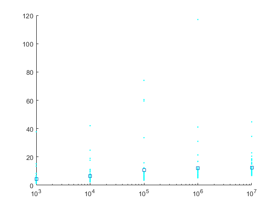
Figure 1: Sample averages of $\det(\dot{X}^{\prime}\dot{X})$
The x-axis indicates sample sizes, there are 50 simulations for each sample size. Averages across simulations for each sample size are in dark blue, their values are $4.28$, $6.63$, $10.6$, $12.1$ and $12.5$.

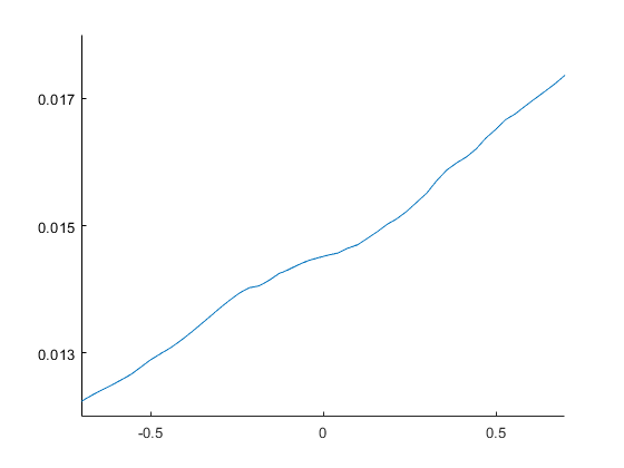
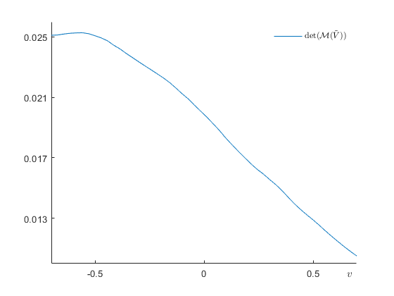
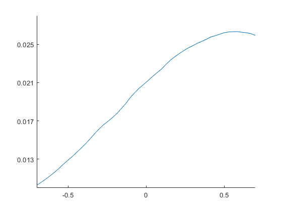
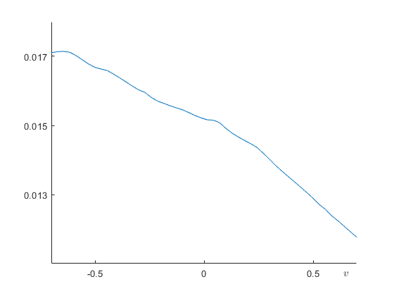
Figure 2: Variations of $\det(\mathcal{M}(\tilde{V}))$
Variations of $\det(\mathcal{M}(\tilde{V}))$ for $v\in[-0.7,0.7]$ and $\tilde{V}=(v,0.5,-0.5,0.5)$ (top left), $\tilde{V}=(-0.5,v,-0.5,0.5)$ (top right), $\tilde{V}=(-0.5,0.5,v,0.5)$ (bottom left), and $\tilde{V}=(-0.5,0.5,-0.5,v)$ (bottom right).

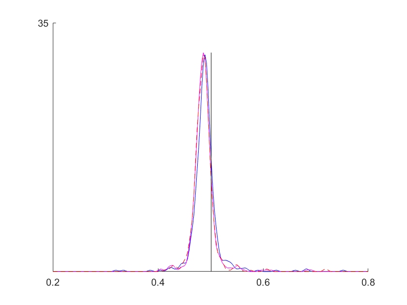
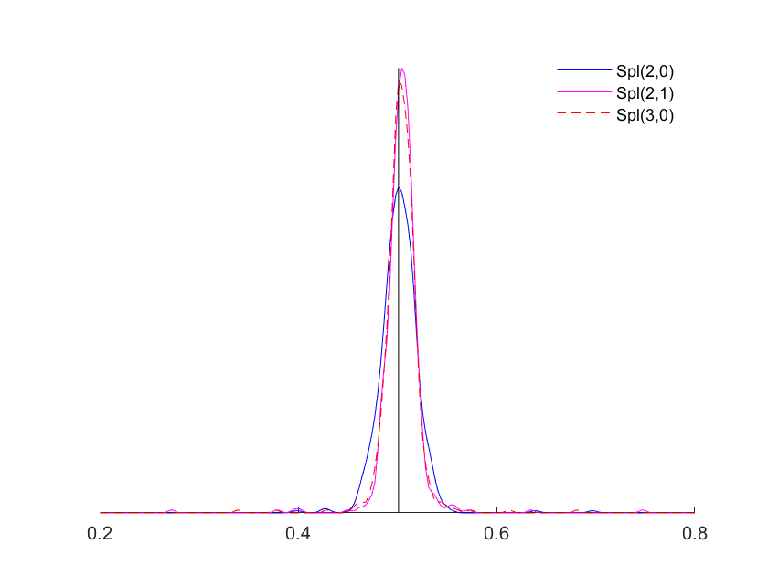
Figure 3: Density of the estimates for $\mu_{1}$
Smoothed histogram of the simulated $\hat{\mu}^{ex}$, for $c=c_{1}$ and $n=5000$. On the left hand side, $f_{t}=s_{t}$ and the right hand side $f_{t}=q_{t}$. The true value $\mathbb{E}(\mu^{ex}|\delta)$ is shown in black.

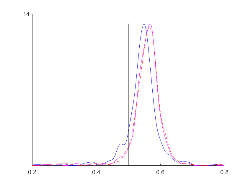
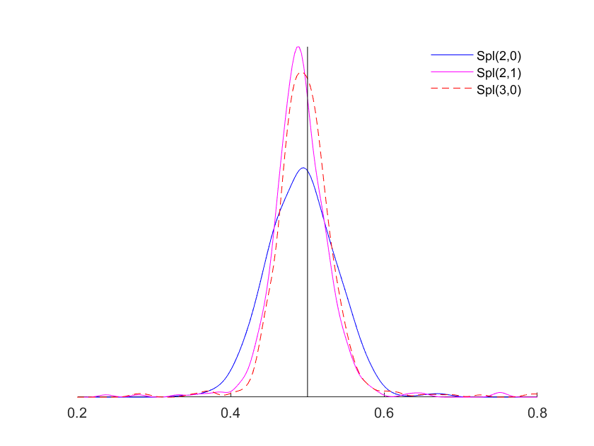
Figure 4: Density of the estimates for $\mu_{2}$
Smoothed histogram of the simulated $\hat{\mu}^{en}$, for $c=c_{1}$ and $n=5000$. On the left hand side, $f_{t}=s_{t}$ and the right hand side $f_{t}=q_{t}$. The true value $\mathbb{E}(\mu^{en}|\delta)$ is shown in black.

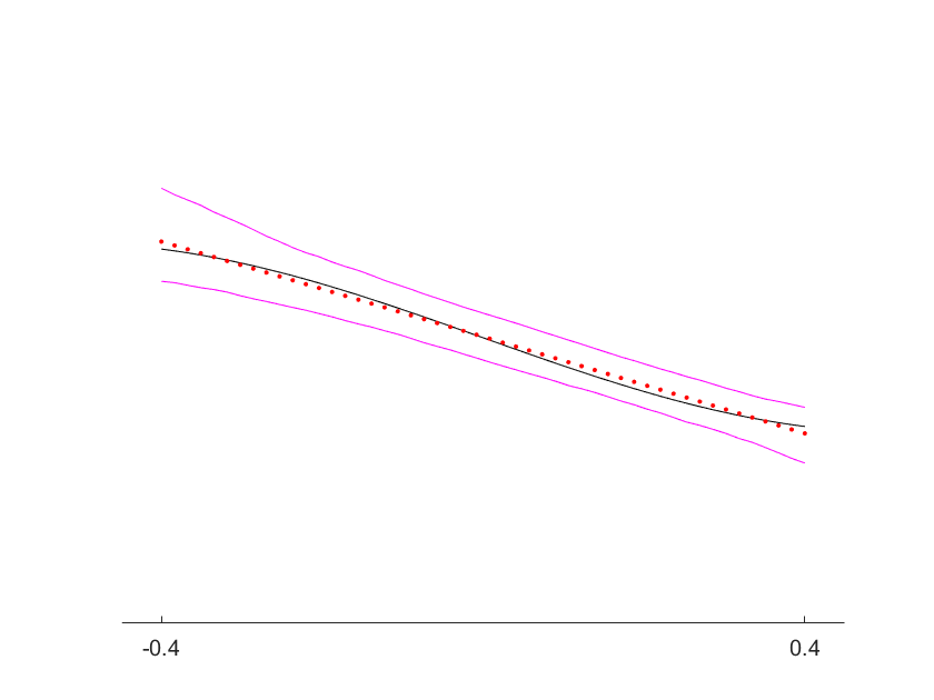
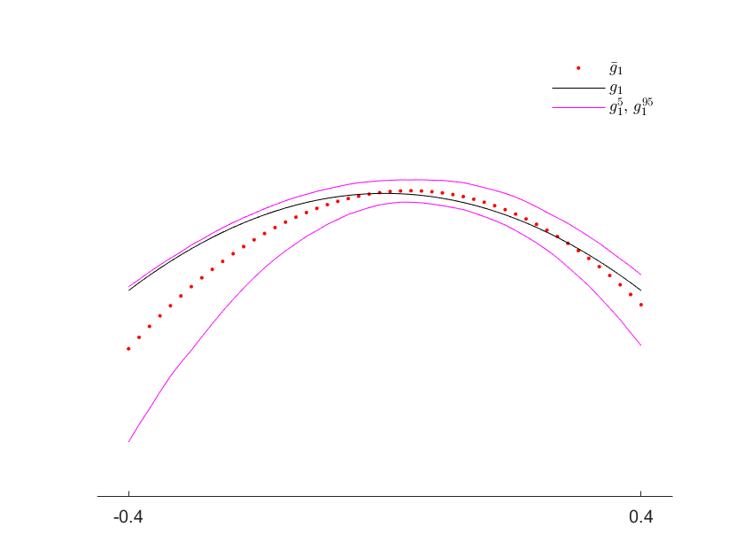
Figure 5: Nonparametric estimation of $g_{1}$
Plot of the pointwise average $\bar{g}_{1}$, the 90 percent MC confidence bands $g_{1}^{5}$ and $g_{1}^{95}$ and the true value $g_{1}$, for $c=c_{1}$ and $n=5000$. On the left hand side, $f_{t}=s_{t}$ and the right hand side $f_{t}=q_{t}$.

References

- (1)
- Abadir and Magnus (2005) Abadir, K. M. and Magnus, J. R. (2005), Matrix algebra, Vol. 1, Cambridge University Press.
- Abrevaya (2006) Abrevaya, J. (2006), ‘Estimating the effect of smoking on birth outcomes using a matched panel data approach’, Journal of Applied Econometrics 21(4), 489–519.
- Ackerberg et al. (2015) Ackerberg, D. A., Caves, K. and Frazer, G. (2015), ‘Identification properties of recent production function estimators’, Econometrica 83(6), 2411–2451.
- Ahn and Powell (1993) Ahn, H. and Powell, J. L. (1993), ‘Semiparametric estimation of censored selection models with a nonparametric selection mechanism’, Journal of Econometrics 58(1-2), 3–29.
- Ai and Chen (2003) Ai, C. and Chen, X. (2003), ‘Efficient estimation of models with conditional moment restrictions containing unknown functions’, Econometrica 71(6), 1795–1843.
- Altonji and Matzkin (2005) Altonji, J. G. and Matzkin, R. L. (2005), ‘Cross section and panel data estimators for nonseparable models with endogenous regressors’, Econometrica 73(4), 1053–1102.
- Andrews (1991) Andrews, D. W. (1991), ‘Asymptotic normality of series estimators for nonparametric and semiparametric regression models’, Econometrica: Journal of the Econometric Society pp. 307–345.
- Arellano (2003) Arellano, M. (2003), Panel data econometrics, Oxford university press.
- Arellano et al. (2017) Arellano, M., Blundell, R. and Bonhomme, S. (2017), ‘Earnings and consumption dynamics: a nonlinear panel data framework’, Econometrica 85(3), 693–734.
- Arellano and Bonhomme (2012) Arellano, M. and Bonhomme, S. (2012), ‘Identifying distributional characteristics in random coefficients panel data models’, The Review of Economic Studies 79(3), 987–1020.
- Arellano and Bonhomme (2016) Arellano, M. and Bonhomme, S. (2016), ‘Nonlinear panel data estimation via quantile regressions’, The Econometrics Journal 19(3), C61–C94.
- Arellano and Honoré (2001) Arellano, M. and Honoré, B. (2001), Panel data models: some recent developments, in ‘Handbook of econometrics’, Vol. 5, Elsevier, pp. 3229–3296.
- Arkhangelsky and Imbens (2018) Arkhangelsky, D. and Imbens, G. (2018), ‘The role of the propensity score in fixed effect models’, arXiv preprint arXiv:1807.02099 .
- Bester and Hansen (2009) Bester, C. A. and Hansen, C. (2009), ‘Identification of marginal effects in a nonparametric correlated random effects model’, Journal of Business & Economic Statistics 27(2), 235–250.
- Blundell and Powell (2003) Blundell, R. W. and Powell, J. L. (2003), Endogeneity in Nonparametric and Semiparametric Regression Models, Vol. 2 of Econometric Society Monographs, Cambridge University Press, p. 312–357.
- Blundell and Powell (2004) Blundell, R. W. and Powell, J. L. (2004), ‘Endogeneity in semiparametric binary response models’, The Review of Economic Studies 71(3), 655–679.
- Card (2001) Card, D. (2001), ‘Estimating the return to schooling: Progress on some persistent econometric problems’, Econometrica 69(5), 1127–1160.
- Chamberlain (1992) Chamberlain, G. (1992), ‘Efficiency bounds for semiparametric regression’, Econometrica 60(3), 567–596.
- Chen et al. (2005) Chen, X., Hong, H. and Tamer, E. (2005), ‘Measurement error models with auxiliary data’, The Review of Economic Studies 72(2), 343–366.
- Chen et al. (2008) Chen, X., Hong, H. and Tarozzi, A. (2008), ‘Semiparametric efficiency in gmm models with auxiliary data’, The Annals of Statistics 36(2), 808–843.
- Chen et al. (2003) Chen, X., Linton, O. and Van Keilegom, I. (2003), ‘Estimation of semiparametric models when the criterion function is not smooth’, Econometrica 71(5), 1591–1608.
- Das et al. (2003) Das, M., Newey, W. K. and Vella, F. (2003), ‘Nonparametric estimation of sample selection models’, The Review of Economic Studies 70(1), 33–58.
- D’Haultfœuille and Février (2015) D’Haultfœuille, X. and Février, P. (2015), ‘Identification of nonseparable triangular models with discrete instruments’, Econometrica 83(3), 1199–1210.
- Escanciano et al. (2016) Escanciano, J. C., Jacho-Chávez, D. and Lewbel, A. (2016), ‘Identification and estimation of semiparametric two-step models’, Quantitative Economics 7(2), 561–589.
- Escanciano et al. (2014) Escanciano, J. C., Jacho-Chávez, D. T. and Lewbel, A. (2014), ‘Uniform convergence of weighted sums of non and semiparametric residuals for estimation and testing’, Journal of Econometrics 178, 426–443.
- Evans and Ringel (1999) Evans, W. N. and Ringel, J. S. (1999), ‘Can higher cigarette taxes improve birth outcomes?’, Journal of public Economics 72(1), 135–154.
- Evdokimov (2010) Evdokimov, K. (2010), ‘Identification and estimation of a nonparametric panel data model with unobserved heterogeneity’, Department of Economics, Princeton University .
- Fernandez-Val et al. (2022) Fernandez-Val, I., Gao, W. Y., Liao, Y. and Vella, F. (2022), ‘Dynamic heterogeneous distribution regression panel models, with an application to labor income processes’, arXiv preprint arXiv:2202.04154 .
- Florens et al. (2008) Florens, J.-P., Heckman, J. J., Meghir, C. and Vytlacil, E. (2008), ‘Identification of treatment effects using control functions in models with continuous, endogenous treatment and heterogeneous effects’, Econometrica 76(5), 1191–1206.
- French (2004) French, E. (2004), ‘The labor supply response to (mismeasured but) predictable wage changes’, Review of Economics and Statistics 86(2), 602–613.
- Gollin and Udry (2021) Gollin, D. and Udry, C. (2021), ‘Heterogeneity, measurement error, and misallocation: Evidence from african agriculture’, Journal of Political Economy 129(1), 1–80.
- Graham et al. (2018) Graham, B. S., Hahn, J., Poirier, A. and Powell, J. L. (2018), ‘A quantile correlated random coefficients panel data model’, Journal of Econometrics 206(2), 305–335.
- Graham and Powell (2012) Graham, B. S. and Powell, J. L. (2012), ‘Identification and estimation of average partial effects in “irregular” correlated random coefficient panel data models’, Econometrica 80(5), 2105–2152.
- Hahn et al. (2018) Hahn, J., Liao, Z. and Ridder, G. (2018), ‘Nonparametric two-step sieve m estimation and inference’, Econometric Theory pp. 1–44.
- Hahn and Ridder (2013) Hahn, J. and Ridder, G. (2013), ‘Asymptotic variance of semiparametric estimators with generated regressors’, Econometrica 81(1), 315–340.
- Hahn and Ridder (2019) Hahn, J. and Ridder, G. (2019), ‘Three-stage semi-parametric inference: Control variables and differentiability’, Journal of econometrics 211(1), 262–293.
- Heckman and Vytlacil (1998) Heckman, J. and Vytlacil, E. (1998), ‘Instrumental variables methods for the correlated random coefficient model: Estimating the average rate of return to schooling when the return is correlated with schooling’, Journal of Human Resources pp. 974–987.
- Hoderlein and White (2012) Hoderlein, S. and White, H. (2012), ‘Nonparametric identification in nonseparable panel data models with generalized fixed effects’, Journal of Econometrics 168(2), 300–314.
- Holtz-Eakin et al. (1988) Holtz-Eakin, D., Newey, W. and Rosen, H. S. (1988), ‘Estimating vector autoregressions with panel data’, Econometrica: Journal of the econometric society pp. 1371–1395.
- Honoré and Kyriazidou (2000) Honoré, B. E. and Kyriazidou, E. (2000), ‘Panel data discrete choice models with lagged dependent variables’, Econometrica 68(4), 839–874.
- Horn and Johnson (2012) Horn, R. A. and Johnson, C. R. (2012), Matrix analysis, Cambridge university press.
- Hoxby (2000) Hoxby, C. M. (2000), ‘The effects of class size on student achievement: New evidence from population variation’, The Quarterly Journal of Economics 115(4), 1239–1285.
- Hsiao (2014) Hsiao, C. (2014), Analysis of Panel Data, Econometric Society Monographs, 3 edn, Cambridge University Press.
- Hu and Schennach (2008) Hu, Y. and Schennach, S. M. (2008), ‘Instrumental variable treatment of nonclassical measurement error models’, Econometrica 76(1), 195–216.
- Ichimura and Lee (2010) Ichimura, H. and Lee, S. (2010), ‘Characterization of the asymptotic distribution of semiparametric m-estimators’, Journal of Econometrics 159(2), 252–266.
- Imbens (2007) Imbens, G. W. (2007), ‘Nonadditive models with endogenous regressors’, Econometric Society Monographs 43, 17.
- Imbens and Newey (2009) Imbens, G. W. and Newey, W. K. (2009), ‘Identification and estimation of triangular simultaneous equations models without additivity’, Econometrica 77(5), 1481–1512.
- Jovanovic (1979) Jovanovic, B. (1979), ‘Job matching and the theory of turnover’, Journal of political economy 87(5, Part 1), 972–990.
- Kumar and Liang (2020) Kumar, A. and Liang, C.-Y. (2020), ‘Estimating taxable income responses with elasticity heterogeneity’, Journal of Public Economics 188, 104209.
- Laird and Ware (1982) Laird, N. M. and Ware, J. H. (1982), ‘Random-effects models for longitudinal data’, Biometrics pp. 963–974.
- Li (2021) Li, M. (2021), ‘A time-varying endogenous random coefficient model with an application to production functions’, arXiv preprint arXiv:2110.00982 .
- Liu et al. (2021) Liu, L., Poirier, A. and Shiu, J.-L. (2021), ‘Identification and estimation of average partial effects in semiparametric binary response panel models’, arXiv preprint arXiv:2105.12891 .
- MaCurdy (1985) MaCurdy, T. E. (1985), ‘Interpreting empirical models of labor supply in an intertemporal framework with uncertainty’, Longitudinal analysis of labor market data pp. 148–170.
- Mairesse and Griliches (1988) Mairesse, J. and Griliches, Z. (1988), ‘Heterogeneity in panel data: are there stable production functions?’.
- Mammen et al. (2016) Mammen, E., Rothe, C. and Schienle, M. (2016), ‘Semiparametric estimation with generated covariates’, Econometric Theory 32(5), 1140–1177.
- Masten and Torgovitsky (2016) Masten, M. A. and Torgovitsky, A. (2016), ‘Identification of instrumental variable correlated random coefficients models’, Review of Economics and Statistics 98(5), 1001–1005.
- Maurer et al. (2011) Maurer, J., Klein, R. and Vella, F. (2011), ‘Subjective health assessments and active labor market participation of older men: evidence from a semiparametric binary choice model with nonadditive correlated individual-specific effects’, Review of Economics and Statistics 93(3), 764–774.
- Miller (1984) Miller, R. A. (1984), ‘Job matching and occupational choice’, Journal of Political economy 92(6), 1086–1120.
- Murtazashvili and Wooldridge (2008) Murtazashvili, I. and Wooldridge, J. M. (2008), ‘Fixed effects instrumental variables estimation in correlated random coefficient panel data models’, Journal of Econometrics 142(1), 539–552.
- Murtazashvili and Wooldridge (2016) Murtazashvili, I. and Wooldridge, J. M. (2016), ‘A control function approach to estimating switching regression models with endogenous explanatory variables and endogenous switching’, Journal of Econometrics 190(2), 252–266.
- Newey (1994a) Newey, W. K. (1994a), ‘The asymptotic variance of semiparametric estimators’, Econometrica: Journal of the Econometric Society pp. 1349–1382.
- Newey (1994b) Newey, W. K. (1994b), ‘Kernel estimation of partial means and a general variance estimator’, Econometric Theory 10(2), 1–21.
- Newey (1997) Newey, W. K. (1997), ‘Convergence rates and asymptotic normality for series estimators’, Journal of econometrics 79(1), 147–168.
- Newey (2009) Newey, W. K. (2009), ‘Two-step series estimation of sample selection models’, The Econometrics Journal 12, S217–S229.
- Newey et al. (1999) Newey, W. K., Powell, J. L. and Vella, F. (1999), ‘Nonparametric estimation of triangular simultaneous equations models’, Econometrica 67(3), 565–603.
- Newey and Stouli (2018) Newey, W. K. and Stouli, S. (2018), ‘Heterogenous coefficients, discrete instruments, and identification of treatment effects’, arXiv preprint arXiv:1811.09837 .
- Newey and Stouli (2021) Newey, W. and Stouli, S. (2021), ‘Control variables, discrete instruments, and identification of structural functions’, Journal of Econometrics 222(1), 73–88.
- Pakes and Ericson (1998) Pakes, A. and Ericson, R. (1998), ‘Empirical implications of alternative models of firm dynamics’, Journal of economic theory 79(1), 1–45.
- Pesaran and Smith (1995) Pesaran, M. H. and Smith, R. (1995), ‘Estimating long-run relationships from dynamic heterogeneous panels’, Journal of econometrics 68(1), 79–113.
- Robinson (1988) Robinson, P. M. (1988), ‘Root-n-consistent semiparametric regression’, Econometrica: Journal of the Econometric Society pp. 931–954.
- Sasaki and Ura (2021) Sasaki, Y. and Ura, T. (2021), ‘Slow movers in panel data’, arXiv preprint arXiv:2110.12041 .
- Suri (2011) Suri, T. (2011), ‘Selection and comparative advantage in technology adoption’, Econometrica 79(1), 159–209.
- Swamy (1970) Swamy, P. A. (1970), ‘Efficient inference in a random coefficient regression model’, Econometrica: Journal of the Econometric Society pp. 311–323.
- Tian (2002) Tian, Y. (2002), ‘The dimension of intersection of subspaces’, Missouri Journal of Mathematical Sciences 14(2), 92–95.
- Torgovitsky (2015) Torgovitsky, A. (2015), ‘Identification of nonseparable models using instruments with small support’, Econometrica 83(3), 1185–1197.
- Verdier (2020) Verdier, V. (2020), ‘Average treatment effects for stayers with correlated random coefficient models of panel data’, Journal of Applied Econometrics 35(7), 917–939.
- Wooldridge (1995) Wooldridge, J. M. (1995), ‘Selection corrections for panel data models under conditional mean independence assumptions’, Journal of econometrics 68(1), 115–132.
- Wooldridge (1997) Wooldridge, J. M. (1997), ‘On two stage least squares estimation of the average treatment effect in a random coefficient model’, Economics letters 56(2), 129–133.
- Wooldridge (2003) Wooldridge, J. M. (2003), ‘Further results on instrumental variables estimation of average treatment effects in the correlated random coefficient model’, Economics letters 79(2), 185–191.
- Wooldridge (2005a) Wooldridge, J. M. (2005a), ‘Fixed-effects and related estimators for correlated random-coefficient and treatment-effect panel data models’, Review of Economics and Statistics 87(2), 385–390.
- Wooldridge (2005b) Wooldridge, J. M. (2005b), ‘Instrumental variables estimation with panel data’, Econometric Theory 21(4), 865–869.
- Wooldridge (2005c) Wooldridge, J. M. (2005c), Unobserved Heterogeneity and Estimation of Average Partial Effects, Cambridge University Press, p. 27–55.
- Ziliak (1997) Ziliak, J. P. (1997), ‘Efficient estimation with panel data when instruments are predetermined: an empirical comparison of moment-condition estimators’, Journal of Business & Economic Statistics 15(4), 419–431.