Chaotic diffusion for particles moving in a time dependent potential well

Abstract

The chaotic diffusion for particles moving in a time dependent potential well is described by using two different procedures: (i) via direct evolution of the mapping describing the dynamics and ; (ii) by the solution of the diffusion equation. The dynamic of the diffusing particles is made by the use of a two dimensional, nonlinear area preserving map for the variables energy and time. The phase space of the system is mixed containing both chaos, periodic regions and invariant spanning curves limiting the diffusion of the chaotic particles. The chaotic evolution for an ensemble of particles is treated as random particles motion and hence described by the diffusion equation. The boundary conditions impose that the particles can not cross the invariant spanning curves, serving as upper boundary for the diffusion, nor the lowest energy domain that is the energy the particles escape from the time moving potential well. The diffusion coefficient is determined via the equation of the mapping while the analytical solution of the diffusion equation gives the probability to find a given particle with a certain energy at a specific time. The momenta of the probability describe qualitatively the behavior of the average energy obtained by numerical simulation, which is investigated either as a function of the time as well as some of the control parameters of the problem.

I Introduction

Diffusive processes are observed in a wide variety of systems ranging from pollen diffusing from plant to plant paper1 , in medicine to the investigation of drugs delivered through the blood current paper2 , how diseases propagate in the air africa ; malaria1 ; malaria2 , population movements in European prehistory culture , pollution in atmosphere paper3 and in the oceans paper4 , percolation paper5 with the investigation of the chemical compounds being transported to the water table, memes in social media diego , the influence of the clime in pests spreading pests and many other applications from physical side paper6 ; paper7 ; paper8 turning the topic of interest to many paper9 ; paper10 ; paper11 .

In this paper we study the diffusion of chaotic orbits where particles are confined to move in a time dependent potential well paper12 ; paper13 . The physical motivation of such a potential paper14 comes from the interaction of photons with the array of atoms producing phonons in the chain leading to oscillations of the bottom part of the potential. The array is composed of infinitely many symmetric wells that can be modeled, due to the symmetry, by a single oscillating potential paper15 . The dynamic of each particle is made by the use of a two dimensional mapping given by energy of the particle and the corresponding time when it leaves the oscillating well. The oscillating part is characterized by three relevant control parameters, one gives the length of the well, other gives its depth and a third one gives the frequency of oscillation. The constant part of the potential has a parameter giving its length, which shall be considered symmetric with the time moving part. The phase space of the model is mixed and contains a set of periodic islands surrounded by a chaotic sea limited by a set of invariant spanning curves. Since the determinant of the Jacobian matrix is the unity, the particles moving in the chaotic sea can not penetrate the islands nor cross through the invariant spanning curve paper16 at the cost of violating the Liouville’s paper6 theorem. The chaotic orbits diffuse along the chaotic sea and they behave similar to random walk particles at such a region. To describe their diffusion we solve the diffusion equation paper7 imposing that the flux of particles through the lowest energy invariant spanning curve is null as well as it is null in lower part of the phase space, where the particle reaches minimal energy to move outside of the time dependent part of the potential. The initial conditions are chosen all with a fixed energy $e_{0}$ and considering an ensemble of particles with such energy but with different phases of the moving potential. The solution of the diffusion equation paper7 gives the probability to find a given particle with a specific energy in a given time. From the knowledge of the probability, we obtain their momenta as functions of the time and compare with the numerical simulations. As we shall see, the qualitative agreement of the curves describing the diffusion is remarkable showing difference at the stationary state, a behavior obtained for long enough time. As we discuss along the text, such a difference is mostly connected to the shape of the phase space where islands are present surrounded by chaotic sea. As an assumption for the solution of the diffusion equation, such islands are not taken into account paper11 and their existence change the saturation of the curves for the diffusion at long enough time. We estimate the fraction that the islands occupy in the phase space and use it to made a first order correction in the saturation of the curves as an attempt to consider the same density of points in the phase space generated by the set of equations of the mapping and that used in the solution of the diffusion equation.

This paper is organized as follows. In Section II we describe the equations of the mapping, construct the phase space and describe the estimation of the lowest energy invariant spanning curve. Section III is devoted to discuss the results for the diffusion equation. Conclusion and final remarks are drawn in Section IV.

II The model, the mapping and some dynamical properties

The dynamical model we consider consists of an ensemble of non interacting particles confined to move inside a potential well described by $V(x,t)=V_{0}(x)+V_{1}(x,t)$ where

$$V_{0}(x)=\left\{\begin{array}[]{ll}V_{0}~{}~{}~{}{\rm if}~{}~{}~{}0<x<{{b}\over{2}}~{}~{}{\rm and}~{}~{}a+{{b}\over{2}}<x<a+b\\ ~{}0~{}~{}~{}{\rm if}~{}~{}~{}{{b}\over{2}}\leq x\leq a+{{b}\over{2}}\\ \infty~{}~{}~{}{\rm if}~{}~{}~{}x\leq 0~{}~{}{\rm and}~{}~{}x\geq a+b\end{array}\right.$$

and $V_{1}(x,t)$ is written as

$$V_{1}(x,t)=\left\{\begin{array}[]{ll}~{}0~{}~{}~{}{\rm if}~{}~{}~{}x<{{b}\over{2}}~{}~{}{\rm and}~{}~{}x>a+{{b}\over{2}}\\ d\cos(\omega t)~{}~{}~{}{\rm if}~{}~{}~{}{{b}\over{2}}\leq x\leq a+{{b}\over{2}}\end{array}\right..$$

Figure 1 shows a plot of the potential.

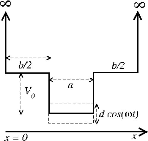
Figure 1: Sketch of the potential.

The dynamic of the particle is described by a two dimensional mapping written in terms of the energy and phase of the moving wall when it leaves the oscillating well. A careful discussion of the construction of the mapping can be found in Refs map1 ; map2 ; map3 . The expression of the mapping is given by

$$T:\left\{\begin{array}[]{ll}e_{n+1}=e_{n}+\delta[\cos(\phi_{n}+i\Delta\phi_{a})-\cos(\phi_{n})],\\ \phi_{n+1}=[\phi_{n}+i\Delta\phi_{a}+\Delta\phi_{b}]~{}~{}{\rm mod(2\pi)},\\ \end{array}\right.$$ (1)

where $e_{n}=E_{n}/V_{0}$, $\Delta\phi_{a}={{2\pi N_{c}}\over{\sqrt{e_{n}-\delta\cos(\phi_{n})}}}$ and $\Delta\phi_{b}={{2\pi N_{c}r}\over{\sqrt{e_{n+1}-1}}}$ with $r=b/a$, $\delta=d/V_{0}$ and $N_{c}={{\omega}\over{2\pi}}{{a}\over{\sqrt{2V_{0}/m}}}$. The parameter $N_{c}$ corresponds to the number of oscillations the potential well completes in the interval of time a particle travels the distance $a$ with kinetic energy $K=V_{0}$. Since it is proportional to $\omega$, increasing $N_{c}$ is equivalent to increase the driving frequency of the potential well. The variable $i$ corresponds to the smallest integer number, $i=1,2,3\ldots$ that satisfies the condition $e_{n}+\delta[\cos(\phi_{n}+i\Delta\phi_{a})-\cos(\phi_{n})]>1$ (see Ref. paper15 ; reflection1 for a discussion on the number of successive reflections in the well). Figure 2 shows a plot of the phase space for the mapping (1) considering the control parameters $r=1$, $\delta=0.5$ and $N_{c}=50$.

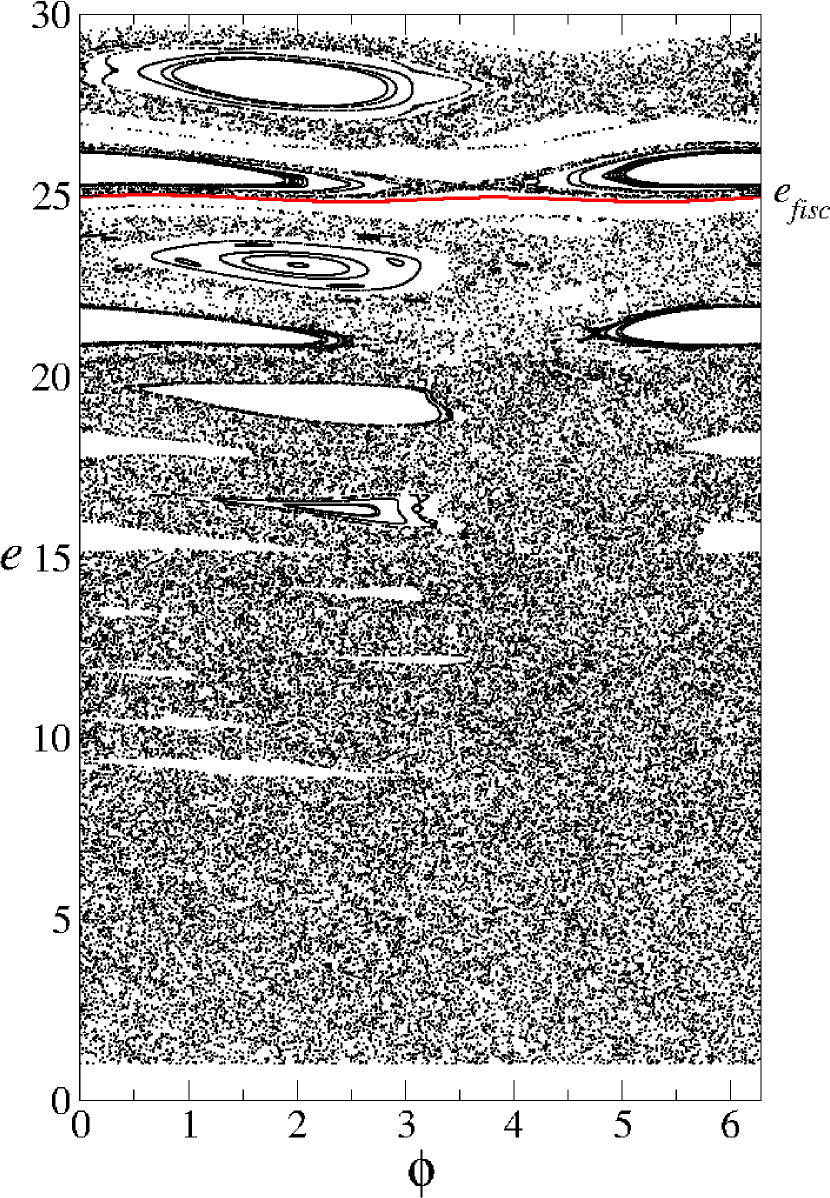
Figure 2: Plot of the phase space for mapping (1) for the parameters: $r=1$, $\delta=0.5$ and $N_{c}=50$. The continuous curve identifies the position of the lowest energy invariant spanning curve, marking the upper limit of the chaotic sea.

We see a mixed structure of the phase space containing both periodic islands, a chaotic sea that is limited by a lowest energy invariant spanning curve. Such curve works as a barrier blocking the passage of particles through it confining the chaotic sea and defining an upper bound for the diffusion. The lower part is defined by the minimal energy the particle needs to escape the moving potential well, i.e., $e_{min}=1$. Therefore, the chaotic sea is limited to the range $e\in[e_{min},e_{fisc}]$. Along this paper we choose the parameter $r=1$ that characterizes the symmetric case. The two parameters we choose to vary are $\delta$ and $N_{c}$. The first parameter, $\delta\in[0,1]$ defines the amplitude of the oscillating well while the latter is proportional to the frequency of oscillation of the moving well, hence a parameter giving how fast the movement of the time dependent potential is.

The observable we are interested in investigate and that gives the characteristics of the diffusion is defined as

$$e_{rms}(n)=\sqrt{{{1}\over{M}}\sum_{i=1}^{M}\frac{1}{n}\sum_{j=1}^{n}e^{2}_{i,j}(n)},$$ (2)

where $M$ gives the size of the ensemble of different initial phases $\phi_{0}\in[0,2\pi]$ and $n$ is the number of iterations of the map. A typical behavior of the curves of $e_{rms}~{}vs.~{}n$ is shown in Fig. 3 for the parameters $N_{c}\in[10^{1},10^{4}]$ and $\delta=0.25$ for the symmetrical case of $r=1$.

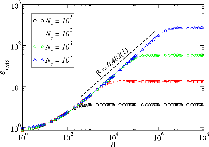
Figure 3: Plot of the curves of $e_{rms}~{}vs.~{}n$ for different values of $N_{c}\in[10^{1},10^{4}]$ and $\delta=0.25$ for the symmetrical case $r=1$.

We see from Fig. 3 that the curves of $e_{rms}$ start to growth in power law in $n$. A power law fitting of the regime of acceleration furnishes an exponent $\beta=0.482(1)$ which is very close to the exponent measured in normal diffusion for random walk particles. The saturation of the curves depends on the position of the lowest energy invariant spanning curve. Since the curves of $\lim_{n\rightarrow\infty}e_{rms}(n)$ depend on the size of the chaotic sea, the localization of the invariant spanning curves plays a major rule on the diffusion. Figure 4 shows a plot of the average energy of the lowest energy invariant spanning curve.

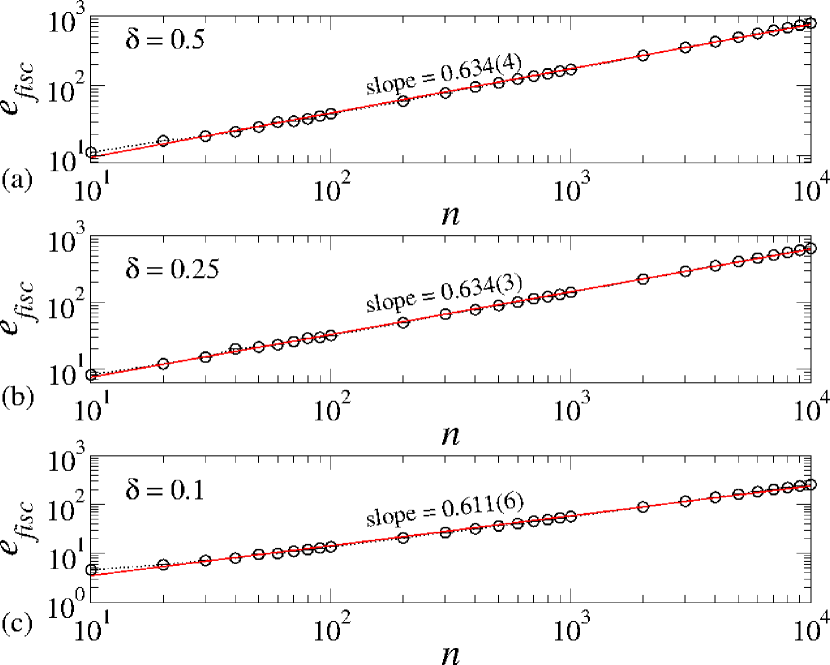
Figure 4: Plot of the average energy of the lowest energy invariant spanning curve. The parameters used were $r=1$, $N_{c}\in[10^{1},10^{4}]$ and: (a) $\delta=0.5$, (b) $\delta=0.25$ and (c) $\delta=0.1$.

The results shown in Fig. 4 are in well agreement with the ones already known from the scaling theory paper15 where the formalism is based on three scaling hypotheses juliano and from the localization of the invariant spanning curves spanning . Starting with low initial energy, it gives the ensemble of particles the chance of experience the larger diffusion as possible. At this domain of energy, the behavior of $e_{rms}(n)$ is described by: (i) for short $n$, the curves exhibit diffusion such that $e_{rms}(n)\propto n^{\beta}$, hence the particles diffuse with slope $\beta\cong 0.5$. This numerical value gives evidence that the ensemble of chaotic particles are diffusing such as random particles. (ii) For large enough $n$, the particles visit a vast part of the phase space such that the curve of $\lim_{n\rightarrow\infty}e_{rms}(n)$ approaches a regime of saturation marked by $\lim_{n\rightarrow\infty}e_{rms}(n)\propto N_{c}^{\alpha}$. The numerical value obtained for such a behavior is from the order of $2/3$, hence in agreement with the description of the invariant spanning curves spanning . The changeover from growth to the saturation is given by $n_{x}\propto N_{c}^{z}$. These scaling hypotheses allow to describe $e_{rms}$ as a homogeneous and generalized function yielding in the following scaling law $z=\alpha/\beta$. Therefore, $z\cong 4/3$. This investigation is phenomenological, so far. In the next section we provide a discussion that involves the solution of the diffusion equation paper7 . From such a solution, the momenta of the distribution are obtained and the critical exponents appear in an analytical way. As we shall see the existence of the islands affects the saturation of the curves by using the diffusion equation while compared with the direct simulations from the equations of the motion. We argue that the fraction of occupied area of chaos is a possible explanation for the difference although the qualitative description of the diffusion equation is remarkable good as compared to the one obtained from the numerical simulations of the dynamical equations.

III The diffusion equation

Since the curves of the average squared energy are well described using scaling formalism, let us now go further and discuss the chaotic diffusion by using the diffusion equation. It is written as

$${{\partial P(e,n)}\over{\partial n}}=D{{\partial^{2}P(e,n)}\over{\partial e^{2}}},$$ (3)

where $P(e,n)$ gives the probability to find a particle with energy $e\in[e_{min},e_{fisc}]$ at a given time $n$. The diffusion coefficient $D$ is obtained from the first equation of mapping (1) by using $D={{\overline{e^{2}}_{n+1}-\overline{e^{2}_{n}}}\over{2}}$. Doing the proper calculations we end up with the result that $D={{\delta^{2}}\over{2}}$.

To obtain an unique solution for Equation (3) we impose the following boundary conditions

$$\left.{{\partial P}\over{\partial e}}\right|_{e=e_{fisc},e_{min}=1}=0,$$ (4)

that guarantee no flux of particles through the invariant spanning curve at $e=e_{fisc}$ and also no flux of particle below the minimal energy $e_{min}=1$. At the initial time, all initial energies are located at $e=e_{0}$ with $e_{min}<e_{0}<e_{fisc}$ and that the probability must satisfy a delta function of the type

$$P(e,0)=\delta(e-e_{0}).$$ (5)

We solved the Equation (3) by the usual method of separation of variables. A solution that satisfies the diffusion equation is

$$P(e,n)=N_{0}e^{-c^{2}n}\left[\tilde{a}\cos\left({{ce}\over{\sqrt{D}}}\right)+\tilde{b}\sin\left({{ce}\over{\sqrt{D}}}\right)\right],$$ (6)

where $N_{0}$, $\tilde{a}$, $\tilde{b}$ and $c$ are constants to be achieved demanding that $P(e,n)$ must satisfy the boundary conditions. At $e=e_{fisc}$ we must have

$${{\tilde{a}}\over{\tilde{b}}}={{\cos\left({{ce_{fisc}}\over{\sqrt{D}}}\right)}\over{\sin\left({{ce_{fisc}}\over{\sqrt{D}}}\right)}},$$ (7)

while at $e_{min}=1$

$${{\tilde{a}}\over{\tilde{b}}}={{\cos\left({{c}\over{\sqrt{D}}}\right)}\over{\sin\left({{c}\over{\sqrt{D}}}\right)}}.$$ (8)

When matching the Equations (7) and (8), we end up with

$$c={{\sqrt{D}k\pi}\over{e_{fisc}-1}},$$ (9)

where $k=1,2,3,\ldots$.

The case $k=0$ must be treated separated and leads to $P(e,n)=\tilde{N_{0}}(E_{0}e+f)$ that must also attend to the boundary conditions with $\tilde{N_{0}}$, $E_{0}$ and $f$ constants. Incorporating the eigenvalue as well as the boundary conditions for any $k$, the probability is written as

$$P(e,n)=a_{0}+\sum_{k=1}^{\infty}\left[a_{k}\cos\left({{k\pi e}\over{e_{fisc}-1}}\right)+b_{k}\sin\left({{k\pi e}\over{e_{fisc}-1}}\right)\right]e^{{{-Dk^{2}\pi^{2}n}\over{(e_{fisc}-1)^{2}}}}.$$ (10)

The next step is then to apply the initial condition at $n=0$. To do that we notice that the delta function can be written by its Fourier series representationbutikov

$$\delta(x)={{1}\over{2\pi}}+{{1}\over{\pi}}\sum_{k=1}^{\infty}\cos(kx).$$ (11)

When we do the transformation $x={{\pi e}\over{e_{fisc}-1}}$, use the property that $\delta(ax)={{1}\over{a}}\delta(x)$ we obtain

$$\delta(e-e_{0})={{1}\over{2(e_{fisc}-1)}}+{{1}\over{(e_{fisc}-1)}}\sum_{k=1}^{\infty}\left[\cos\left({{k\pi e}\over{e_{fisc}-1}}\right)\cos\left({{k\pi e_{0}}\over{e_{fisc}-1}}\right)+\sin\left({{k\pi e}\over{e_{fisc}-1}}\right)\sin\left({{k\pi e_{0}}\over{e_{fisc}-1}}\right)\right].$$ (12)

Comparing Equations (10) and (12) at $n=0$ we obtain that the coefficients are written as

$$a_{0} = {{1}\over{2(e_{fisc}-1)}},$$ (13)

$$a_{k} = {{1}\over{(e_{fisc}-1)}}\cos\left({{k\pi e_{0}}\over{e_{fisc}-1}}\right),$$ (14)

$$b_{k} = {{1}\over{(e_{fisc}-1)}}\sin\left({{k\pi e_{0}}\over{e_{fisc}-1}}\right),$$ (15)

for $k=1,2,3,\ldots$. Using this set of coefficients, the probability given by Eq. (10) is normalized in the range $e\in[e_{min},e_{fisc}]$.

The observable we want to investigate along the chaotic sea producing the chaotic diffusion is defined as $e_{rms}(n)=\sqrt{\overline{e^{2}}(n)}$, where

$$\overline{e^{2}}(n)=\int_{e=1}^{e_{fisc}}e^{2}P(e,n)de.$$ (16)

The expression with all terms of $\overline{e^{2}}(n)$ is presented in the Appendix for the interested reader. From now we limit to consider that

$$\overline{e^{2}}(n)={{e^{3}_{fisc}-1}\over{6(e_{fisc}-1)}}+\sum_{k=1}^{\infty}{{e^{-{{Dk^{2}\pi^{2}n}\over{(e_{fisc}-1)^{2}}}}}\over{(k\pi)^{3}}}[S_{1}+S_{2}+S_{3}+S_{4}].$$ (17)

The term $e_{fisc}$ is not obtained analytically, although numerical results for different values of $\delta$ is plotted in Figure 4.

We discuss the result given in Equation (16). One notices that in the limit of $n\rightarrow\infty$, the exponential term approaches zero, lasting only the distribution for the stationary state, i.e.

$$\lim_{n\rightarrow\infty}e_{rms}(n)=\sqrt{{{e^{3}_{fisc}-1}\over{6(e_{fisc}-1)}}}.$$ (18)

We notice that for $e_{fisc}\gg 1$, $\lim_{n\rightarrow\infty}e_{rms}(n)\cong e_{fisc}/\sqrt{6}$, which is in well agreement with the results shown in Figure 4 hence confirming the saturation exponent $\alpha\cong 2/3$.

Let us now discuss the evolution of $e_{rms}$ for short $n$. Expanding the exponential term of $\sum_{k=1}^{\infty}{{e^{-{{Dk^{2}\pi^{2}n}\over{(e_{fisc}-1)^{2}}}}}\over{(k\pi)^{3}}}$ in Taylor series and considering only the first order approximation when assuming that the leading term of the summation is dominated by $k=1$, we obtain

$$e_{rms}(n)\cong\sqrt{{{e^{3}_{fisc}-1}\over{6(e_{fisc}-1)}}+{{S}\over{\pi^{3}}}-{{SD}\over{\pi(e_{fisc}-1)^{2}}}n},$$ (19)

where $S=S_{1}+S_{2}+S_{3}+S_{4}<0$ with $S_{i}$ for $i=1,2,3,4$ as show in the Appendix considering only the dominant term $k=1$. Therefore prior the saturation, the curves of $e_{rms}(n)\cong\sqrt{-{{SD}\over{\pi(e_{fisc}-1)^{2}}}n}$, hence $\beta=1/2$ as observed in the growing regime.

The regime marking the changeover from growth to the saturation can be estimated by doing $\sqrt{{{e^{3}_{fisc}-1}\over{6(e_{fisc}-1)}}+{{S}\over{\pi^{3}}}-{{SD}\over{\pi(e_{fisc}-1)^{2}}}n}=\sqrt{{{e^{3}_{fisc}-1}\over{6(e_{fisc}-1)}}}$, leading to

$$n_{x}\propto{{(e_{fisc}-1)^{2}}\over{\pi^{2}D}}.$$ (20)

Since $e_{fisc}\propto N_{c}^{\alpha}$, therefore for large $e_{fisc}$ we conclude that the critical exponent $z\cong 4/3$, as known in the literature juliano .

The behavior of $e_{rms}(n)=\sqrt{\overline{e^{2}}(n)}$ obtained from Equation (17) for different values of $N_{c}$ is shown in Figure 5.

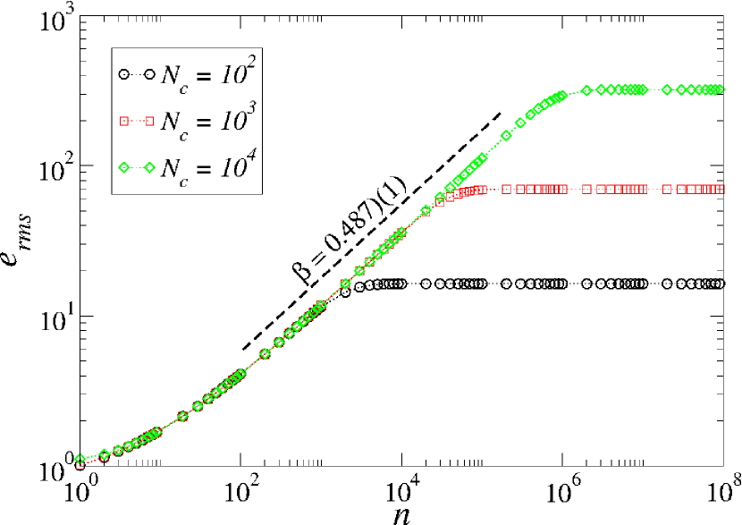
Figure 5: Plot of $e_{rms}(n)~{}vs.~{}n$ for different values of $N_{c}$, as labeled in the figure considering $r=1$ and $\delta=0.5$.

We notice that the regime of growth is mostly marked by a slope of $\beta=0.487(1)\cong 0.5$ when eventually the curves bend towards a regime of saturation as described by Eq. (18).

Let us now compare the analytical results with the numerical simulations. The better way of doing this is by plotting the curves of $e_{rms}(n)$ obtained from the different procedures in the same plot, as shown in Figure 6(a).

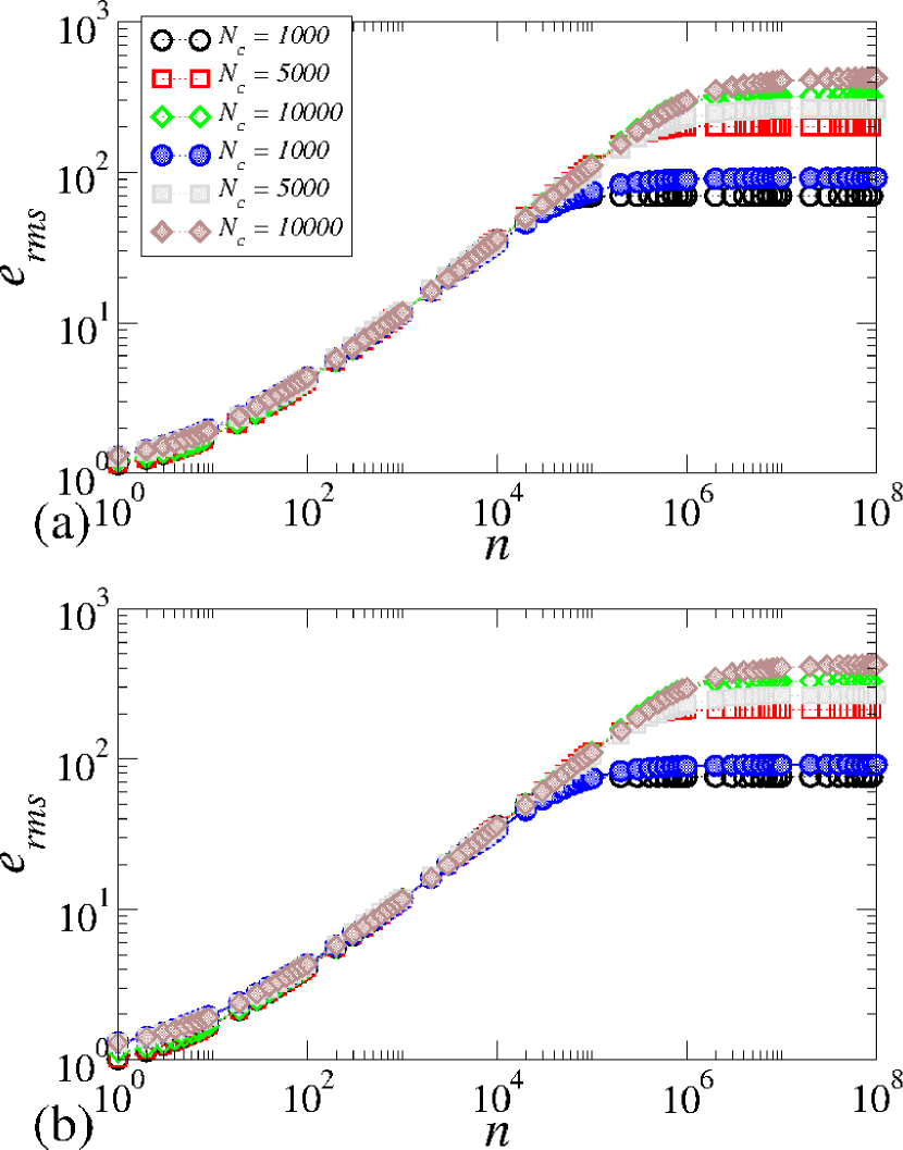
Figure 6: (a) Plot of $e_{rms}(n)~{}vs.~{}n$ for different values of $N_{c}$, as labeled in the figure considering $r=1$ and $\delta=0.5$. Filled symbols correspond to the numerical simulations while open symbols are the analytical results. (b) Same as shown in (a) but using the fraction of occupied phase space from chaotic dynamics.

The filled symbols correspond to the numerical simulations while open symbols are the analytical results. The agreement between the two procedures is remarkable good for short and intermediate values of $n$, either starting with $e_{0}\approx 1$ or larger values of $e_{0}$. The difference lies at the saturation. We now comment on such a difference. From the plot of the phase space, as seen in Figure 2, one can see the existence of the periodicity islands. Since the mapping is area preserving, a chaotic orbit can not penetrate the islands. The orbit moves around it, sometimes getting sticky in such a region and eventually moves away, never getting inside. Because of the existence of the islands, the values of the saturation do not coincide with the half value of the chaotic window. However, at the conception of the boundary conditions in the diffusion equation, we assumed that the phase space is uniformly filled and that the existence of the periodic islands is not taken into account. This may be a possible reason why the curves of $e_{rms}$ constructed from the probability obtained from the diffusion equation saturate at lower values, as compared with the results obtained from the numerical simulations.

To estimate the size of the chaotic sea in the allowed region of the phase space, we obtained the fraction of the area occupied by the chaotic sea for different values of $N_{c}$ and considering three different values of $\delta$. Figure 7 shows a plot

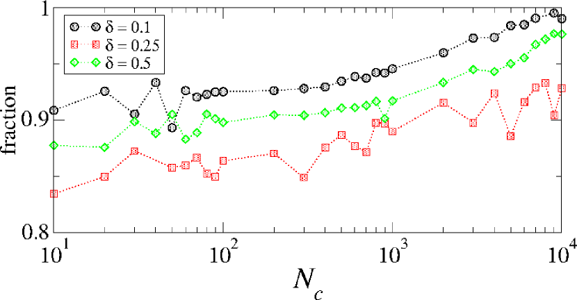
Figure 7: Plot of fraction of area filled by the chaotic sea in the chaotic region of the phase space limited at the range $e\in[e_{min},e_{fisc}]$. The parameters used were $r=1$ and $\delta=0.1$ (circle), $\delta=0.25$ (rectangle) and $\delta=0.5$ (losangle).

of the occupied area of the chaotic sea in the range $e\in[e_{min},e_{fisc}]$. Since the fraction is less than the unity, the density of points considered in the boundary conditions is different from the one assumed in the numerical simulations to that used in the solution of the diffusion equation. To have the same density of points in the phase space that takes into account the existence of the islands, the boundary conditions used in the diffusion equations would request a higher position of the invariant spanning curves. This difference in the density of points in the phase space from the one used in the solution of the diffusion equation is interpreted as being a possible reason for the curves obtained from the two different procedures saturate at distinct places. It is important to mention that such a difference was not observed in Ref. paper11 because the phase space considered there is symmetric with respect to the “action” axis in the positive and negative sides. The islands present in the positive side of $I$ in Ref. paper11 cancel the influence of the islands observed in the negative side of $I$ and such effect does not cause differences in the saturation between the theoretical point of view obtained from the solution of the diffusion equation and the numerical results, obtained directly from the dynamical equations. By using the fraction of the chaotic sea to correct the density of points in the phase space, the curves of $e_{rms}(n)$ obtained from the diffusion equation saturate closer to the ones obtained from numerical simulations, as seen in Fig. 6(b).

IV Conclusions and final remarks

As a summary, we investigate the problem of chaotic diffusion for an ensemble of non interacting particles moving inside a time dependent potential well. The dynamic of each particle is described by an area preserving mapping for the dynamical variables energy and time when the particle leaves the moving well. The phase space is mixed with particles diffusing chaotically along a limited domain given by $e\in[e_{min},e_{fisc}]$. Starting with an initial condition $e_{0}\cong 1$, the curves of $e_{rms}$ growth to start with $n$ in a power law fashion of exponent $\beta\cong 0.5$. This exponent allows to interpret chaotic diffusion similar to random walk particles. The saturation is marked by a power law $\lim_{n\rightarrow\infty}e_{rms}(n)=N_{c}^{\alpha}$ with $\alpha\cong 2/3$ in well agreement with the results known in the literature juliano . The crossover marking the changeover from growth to the saturation is $z\cong 4/3$, also in well agreement with the literature juliano . Our original contribution on this topic comes from the analytical solution of the diffusion equation, that provides a function $P(e,n)$, that is a probability to obtain a given particle with energy $e$ at a specific time $n$. The boundary conditions used imply that the particles can not cross the invariant spanning curves at $e=e_{fisc}$ nor the lowest limit of the energy $e_{min}=1$ at the cost of violating the Liouville’s theorem. The momenta of the distribution are obtained from $P(e,n)$ and compared with the numerical results. We notice a remarkable agreement of the two procedures at short and intermediate time but that the saturation for long enough time happens at different positions. The explanation is related to the existence of islands of stability in the phase space, which are taken into account direct numerical simulations and that are not considered in the solution of the diffusion equation. Although the quantitative results obtained from the two procedures differ from each other at large enough $n$, they show an incredible good agreement for short and intermediate time. The critical exponents obtained from the solution of the diffusion equation are not affected at large enough time, therefore even though the results are slightly different at large $n$, they validate the scaling theory of critical exponents obtained earlier in the literature paper15 . As perspective of the present approach we plan to investigate the chaotic diffusion in dissipative mappings including a dissipative version of the standard mapping and also time dependent billiards when particles experience inelastic collisions with the border of the billiard.

EDL thanks support from CNPq (301318/2019-0) and FAPESP (2019/14038-6), Brazilian agencies. CMK thanks to CAPES for support.

Appendix

Here we present the expression of $\overline{e^{2}}(n)$. It is obtained from $\overline{e^{2}}(n)=\int_{e=1}^{e_{fisc}}e^{2}P(e,n)de$, leading to

$$\overline{e^{2}}(n)={{e^{3}_{fisc}-1}\over{6(e_{fisc}-1)}}+\sum_{k=1}^{\infty}{{e^{-{{Dk^{2}\pi^{2}n}\over{(e_{fisc}-1)^{2}}}}}\over{(k\pi)^{3}}}[S_{1}+S_{2}+S_{3}+S_{4}]$$ (21)

where the auxiliary terms are

$$S_{1} = \cos\left({{k\pi e_{0}}\over{e_{fisc}-1}}\right)\left[\left(\pi^{2}k^{2}e^{2}_{fisc}-2(e_{fisc}-1)^{2}\right)\sin\left({{k\pi e_{fisc}}\over{e_{fisc-1}}}\right)+2\pi(e_{fisc}-1)ke_{fisc}\cos\left({{k\pi e_{fisc}}\over{e_{fisc}-1}}\right)\right],$$

$$S_{2} = \sin\left({{k\pi e_{0}}\over{e_{fisc}-1}}\right)\left[(2(e_{fisc}-1)^{2}-\pi^{2}k^{2}e^{2}_{fisc})\cos\left({{k\pi e_{fisc}}\over{e_{fisc}-1}}\right)+2\pi(e_{fisc}-1)ke_{fisc}\sin\left({{k\pi e_{fisc}}\over{e_{fisc}-1}}\right)\right],$$

$$S_{3} = -\cos\left({{k\pi e_{0}}\over{e_{fisc}-1}}\right)\left[\left(\pi^{2}k^{2}-2(e_{fisc}-1)^{2}\right)\sin\left({{k\pi}\over{e_{fisc-1}}}\right)+2\pi(e_{fisc}-1)k\cos\left({{k\pi}\over{e_{fisc}-1}}\right)\right],$$

$$S_{4} = -\sin\left({{k\pi e_{0}}\over{e_{fisc}-1}}\right)\left[(2(e_{fisc}-1)^{2}-\pi^{2}k^{2})\cos\left({{k\pi}\over{e_{fisc}-1}}\right)+2\pi(e_{fisc}-1)k\sin\left({{k\pi}\over{e_{fisc}-1}}\right)\right].$$

References

- (1) W. F. Morris, Ecology 74, 493 (1993).
- (2) K. Murase, S. Tanada, H. Mogami, M. Kawamura, M. Miyagawa, M. Yamada, H. Higashiro, A. Lio, K. Hamamoto, Medical Physics 19, 70 (1990).
- (3) S. A. El-Kafrawy et al, The Lancet Planetary Health 3, e521 (2019).
- (4) Z. Xu, Y. Zhang, IMA J. of Applied Mathematics 80, 1124 (2015).
- (5) Y. Lou, X. Q. Zhao, J. Math. Biol. 62, 543 (2011).
- (6) E. E. Harris, Evolutionary Anthropology 26, 228 (2017).
- (7) D. Popp, Journal of Environmental Economics and Management 51, 46 (2006).
- (8) R. V. Ozmidov, Diffusion of contaminants in the ocean, Springer (1990).
- (9) C. Hagedorn, E. L. Mc Coy, T. M. Rahe, J. Environ. Qual. 10, 1 (1981).
- (10) X. Qiu, D. F. M. Oliveira, A. S. Shirazi, A. Flammini, F. Menczer, Nature Human Behaviour 1, 0132 (2017).
- (11) W. S. Jo, H. Y. Kim, B. J. Kim, J. Korean Phys. Soc. 70, 108 (2017).
- (12) F. Reif, Fundamentals of statistical and thermal physics, New York: McGraw-Hill (1965).
- (13) V. Balakrishnan, Elements of nonequilibrium statistical mechanics, Ane Books India, New Delhi (2008).
- (14) R. K. Patria, Statistical Mechanics, Elsevier (2008).
- (15) E. D. Leonel, J. Penalva, R. M. N. Teixeira, R. N. Costa Filho, M. R. Silva, J. A. Oliveira, Physics Letters A 379, 1808 (2015).
- (16) A. L. P. Livorati et al, Commun. Nonlinear Sci. Numer. Simulat. 55, 225 (2018).
- (17) E. D. Leonel, C. M. Kuwana, J. Stat. Phys. 170, 69 (2018).
- (18) J. L. Mateos, J. V. José, Physica A 257, 434 (1998).
- (19) J. L. Mateos, Phys. Lett. A 256, 113 (1999).
- (20) G. A. Luna-Acosta, G. Orellana-Rivadeneyra, A. Mendoza- Galván, C. Jung, Chaos, Solitons Fractals 12, 349 (2001).
- (21) D. R. Costa, M. R. Silva, J. A. Oliveira, E. D. Leonel, Physica A 391, 3607 (2012).
- (22) A. J. Lichtenberg, M. A. Lieberman, Regular and chaotic dynamics (Appl. Math. Sci.) 38, Springer Verlag, New York (1992).
- (23) E. D. Leonel, P. V. E. McClintock, Phys. Rev. E 70, 016214 (2004).
- (24) E. D. Leonel, P. V. E. McClintock, Chaos 15, 033701 (2005).
- (25) D. R. da Costa, C. P. Dettmann, E. D. Leonel, Phys. Rev. E 83, 066211 (2011).
- (26) E. D. Leonel, J. K. L. Silva, Physica A 323, 181 (2003).
- (27) J. A. de Oliveira, R. A. Bizão, E. D. Leonel, Phys. Rev. E 81, 046212 (2010).
- (28) E. D. Leonel, J. A. de Oliveira, F. Saif, J. Phys. A 44, 302001 (2011).
- (29) E. Butkov, Mathematical Physics, Addison-Wesley Pub. Co., (1968)