Entropy rigidity for 3D conservative Anosov flows and dispersing billiards

Abstract.

Given an integer $k\geq 5$, and a $C^{k}$ Anosov flow $\Phi$ on some compact connected $3$-manifold preserving a smooth volume, we show that the measure of maximal entropy (MME) is the volume measure if and only if $\Phi$ is $C^{k-\varepsilon}$-conjugate to an algebraic flow, for $\varepsilon>0$ arbitrarily small. Besides the rigidity, we also study the entropy flexibility, and show that the metric entropy with respect to the volume measure and the topological entropy of suspension flows over Anosov diffeomorphisms on the $2$-torus achieve all possible values subject to natural normalizations. Moreover, in the case of dispersing billiards, we show that if the measure of maximal entropy is the volume measure, then the Birkhoff Normal Form of regular periodic orbits with a homoclinic intersection is linear.

1. Introduction

Anosov flows and Anosov diffeomorphisms are among the most well-understood dynamical systems, including the space of invariant measures, stable and unstable distributions and foliations, decay of correlations and other statistical properties. The topological classification of Anosov systems, especially diffeomorphisms, is well-understood in low dimensions. For flows, constructions of “exotic” Anosov flows are often built from gluing several examples of algebraic or geometric origin. Special among them are the algebraic systems, affine systems on homogeneous spaces. In the diffeomorphism case, these are automorphisms of tori and nilmanifolds. Conjecturally, up to topological conjugacy, these account for all Anosov diffeomorphisms (up to finite cover). The case of Anosov flows is quite different. Here, the algebraic models are suspensions of such diffeomorphisms and geodesic flows on negatively curved rank one symmetric spaces. There are many constructions to give new Anosov flows, all of which come from putting together geodesic flows and/or suspensions of diffeomorphisms. In particular, quite unexpected behaviors are possible, including Anosov flows on connected manifolds which are not transitive [FW], analytic Anosov flows that are not algebraic [HT], contact Anosov flows on hyperbolic manifolds that are not topologically orbit equivalent to an algebraic flow [FH], and many other constructions combining these ideas (see, e.g., [BBY]).

When classifying Anosov systems up to $C^{\infty}$ diffeomorphisms, the question becomes very different. Here, the algebraic models are believed to distinguish themselves in many ways, including regularity of dynamical distributions and thermodynamical formalism. In the case of the latter, the first such result was obtained by Katok for geodesic flows of negatively curved surfaces, where it was shown that coincidence of metric entropy with respect to Liouville measure and topological entropy implies that the surface has constant negative curvature [K1, K3]. These works lead to the following conjecture:

Conjecture 1.1 (Katok Entropy Conjecture).

Let $(M,g)$ be a connected Riemannian manifold of negative curvature, and $\Phi$ be the corresponding geodesic flow. Then $h_{\operatorname{top}}(\Phi)=h_{\mu}(\Phi)$ if and only if $(M,g)$ is a locally symmetric space.

A weaker version of this was obtained in higher dimensional geodesic flows under negative curvature assumptions by [BCG], which still highly depends on the structures coming from the geometry of the flow. Other generalizations work with broader classes of Anosov flows. Foulon [Fo] showed that in the case of a contact Anosov flow $\Phi$ on a closed three manifold, $\Phi$ is, up to finite cover, smoothly conjugate to geodesic flow of a metric of constant negative curvature on a closed surface if and only if the measure of maximal entropy is the contact volume. There, he asks the following question generalizing Conjecture 1.1:

Question 1.

Let $\Phi$ be a smooth Anosov flow on a 3-manifold which preserves a smooth volume $\mu$. If $h_{\operatorname{top}}(\Phi)=h_{\mu}(\Phi)$, is $\Phi$ smoothly conjugate to an algebraic flow?

Let us briefly compare Question 1 and Conjecture 1.1. Recall that the geodesic flow on $M$ occurs on the unit tangent bundle, $T^{1}M$, which has dimension $2\dim M-1$. Therefore, Question 1 corresponds to the case of geodesic flows on surfaces, which was proved by Katok in [K1, K3].

The low-dimensionality assumption of Question 1 is required for a theorem in this generality. It is not difficult to construct non-algebraic systems whose maximal entropy measure is a volume when the stable and unstable distributions are multidimensional. This highlights the power of assuming the dynamics is a geodesic flow and why a solution to Conjecture 1.1 would require a mixture of dynamical and geometric ideas.

By contrast, Question 1 is purely dynamical. In particular, it applies to time changes or perturbations of the Handel-Thurston flow [HT] as well as special flows over Anosov diffeomorphisms of ${\mathbb{T}}^{2}$, for which no entropy-rigidity type results were known since they do not preserve contact forms (except for very special cases, see [FH]).

We provide a positive answer to Question 1.

Theorem A.

Let $k\geq 5$ be some integer, and let $\Phi$ be a $C^{k}$ Anosov flow on a compact connected $3$-manifold $M$ such that $\Phi_{*}\mu=\mu$ for some smooth volume $\mu$. Then $h_{\operatorname{top}}(\Phi)=h_{\mu}(\Phi)$ if and only if $\Phi$ is $C^{k-\varepsilon}$-conjugate to an algebraic flow, for $\varepsilon>0$ arbitrarily small.

Moreover, we believe the theorem is true for $k\geq 2$, but technical obstructions prevent us from finding the precise boundary of required regularity. Let us emphasize that regularity is extremely important for the rigidity phenomenon. If one relaxes to the $C^{1}$ category, it is possible to produce examples of flows with quite different behaviour. Indeed, given a $C^{2}$ Axiom A flow on a compact Riemannian manifold and an attractor (see Subsection 2.1 for a definition) whose unstable distribution is $C^{1}$, Parry [Pa] describes a $C^{1}$ time change such that for the new flow, the SRB measure (invariant volume if it exists) of the attractor coincides with the measure of maximal entropy. These measures are obtained as limits of certain closed orbital measures. In particular, for any $C^{2}$ transitive Anosov flow $\Phi$ on a $3$-manifold, the unstable distribution is $C^{1}$ (see Remark 2.3), hence the synchronization procedure explained by Parry shows that $\Phi$ is $C^{1}$-orbit equivalent to a $C^{1}$ Anosov flow for which the SRB measure is equal to the measure of maximal entropy.

Conversely, recent results of Adeboye, Bray and Constantine [ABC] show that systems with more geometric structure still exhibit rigidity in low regularity. In particular, they show a version of the Katok entropy conjecture for geodesic flows on Hilbert geometries, which are only $C^{1+\alpha}$ flows.

Question 1 can be modified to remove the volume preservation assumption. Given any transitive Anosov flow, there are always two natural measures to consider (which fit into a broader class of measures called Gibbs states). One is the measure of maximal entropy, which is the unique measure $\nu$ such that $h_{\nu}(\Phi)=h_{\operatorname{top}}(\Phi)$. The other is the Sinai-Ruelle-Bowen, or SRB measure, which has its conditional measures along unstable manifolds absolutely continuous with respect to Lebesgue. It is therefore natural to consider the following:

Question 2.

Suppose that $\Phi$ is a $C^{\infty}$ transitive Anosov on a 3-manifold. If the SRB measure and MME coincide, is $\Phi$ smoothly conjugate to an algebraic flow?

Our approach is insufficient to answer Question 2, because our method relies on some special change of coordinates introduced by Hurder-Katok [HuKa] for volume-preserving Anosov flows, and on Birkhoff Normal Forms for area-preserving maps (see (1.1) below).

1.1. Outline of arguments and new techniques

The techniques used to prove Theorem A combine several ideas. We do not directly follow the approach of Foulon, who aims to construct a homogeneous structure on the manifold by using a Lie algebra of vector fields tangent to the stable and unstable distributions, together with the vector field generating the flow [Fo]. The central problem in all approaches is the regularity of dynamical distributions. Foulon requires smoothness of the strong stable and unstable distributions, which follows a posteriori from the existence of a smooth conjugacy to an algebraic model, but is often out of reach without additional assumptions, such as a smooth invariant $1$-form.

The main technical result of the paper is the smoothness of the weak foliations. For this we use an invariant of Hurder and Katok [HuKa], the Anosov class, which is an idea that can be dated back to Birkhoff and Anosov. In fact, Anosov used this idea to show the existence of examples for which the regularity of the distributions is low: it was first shown that the invariant is non-trivial, but that it must be trivial in all algebraic examples. Hurder and Katok [HuKa] then proved that vanishing of the invariant implies smoothness of the weak stable and unstable distributions. In the case of an Anosov flow obtained by suspending an Anosov diffeomorphism of the $2$-torus, they showed that it implies smooth conjugacy to an algebraic model. For more regarding the Anosov class and its connection to normal forms for hyperbolic maps, see Subsection 2.3.

For a transitive Anosov flow on some compact connected $3$-manifold, there exists a unique measure of maximal of entropy, or MME. If the MME is equal to the volume measure, we are able to show vanishing of the Anosov class. We deduce from [HuKa] that the weak foliations are smooth. This gives a weaker form of rigidity, due to Ghys [G2]: the existence of a smooth orbit equivalence to an algebraic model. This is not surprising, as taking a time change of any Anosov flow will preserve its weak foliations. With this in hand, there is one last lemma to prove: any time change of an algebraic Anosov flow for which the measure of maximal entropy is equivalent to Lebesgue is smoothly conjugate to a linear time change. This is proved in Proposition 3.11.

The difficulty in proving smoothness using local normal forms is that transverse regularity of stable foliations can’t be controlled locally. We circumvent this problem by using an orbit $h_{\infty}$ homoclinic to a reference periodic orbit $\mathcal{O}$, and a sequence $(h_{n})_{n\geq 0}$ of periodic orbits with prescribed combinatorics shadowing the orbit $h_{\infty}$. We are able to control the dynamical and differential properties of the orbits $(h_{n})_{n\geq 0}$ by choosing an exceptionally good chart (see Subsection 3.2). On the one hand, in Subsection 3.1, we show that for an Axiom A flow restricted to some basic set (see Subsection 2.1 for the definitions), the equality of the MME and of the SRB measure forces the periodic Lyapunov exponents to be equal; by controlling the periods of the orbits $(h_{n})_{n\geq 0}$, this allows us to obtain a first estimate on the Floquet multipliers of the flow for $h_{n}$, $n\geq 0$. On the other hand, by the choice of the orbits $(h_{n})_{n\geq 0}$, we can also study the asymptotics of the Floquet multipliers through the Birkhoff Normal Form of the periodic orbit $\mathcal{O}$ (see Subsection 3.2); the calculations are similar to those in [DKL]. Combining those two estimates, we show the following:

Theorem B.

Let $k\geq 5$ be an integer, and let $\Phi$ be a $C^{k}$ Anosov flow on a $3$-manifold $M$ which preserves a smooth volume $\mu$. If $h_{\operatorname{top}}(\Phi)=h_{\mu}(\Phi)$, then the Anosov class vanishes identically. Moreover, this implies strong rigidity properties:

1. the weak stable/unstable distributions of the flow $\Phi$ are of class $C^{k-3}$;

2. the flow $\Phi$ is $C^{k}$-orbit equivalent to an algebraic model.

Item (1) follows from the vanishing of the Anosov class and the work of Hurder-Katok [HuKa], while (2) follows from (1) and the work of Ghys [G2].

In order to upgrade the orbit equivalence to a smooth flow conjugacy, we use ideas similar to those in Subsection 3.3 of an unpublished paper [Ya] of Yang; indeed, the equality of the MME and of the volume measure allows us to discard bad situations such as those described in [G1]. In Subsection 3.3, we will prove:

Theorem C.

Let $\Phi_{0}$ be an Anosov flow on some $3$-manifold that is a smooth time change of an algebraic flow $\Psi_{0}$. If the measure of maximal entropy of $\Phi_{0}$ is absolutely continuous with respect to volume, then $\Phi_{0}$ is a linear time change of $\Psi_{0}$.

In other words, up to a linear time change, the periods of associated periodic orbits for the flow and the algebraic model coincide. By Livsic’s theorem, this allows us to synchronize the orbit equivalence, and produce a conjugacy between the two flows; the smoothness of this conjugacy is automatic (it follows from previous rigidity results in [dlL]). In particular, Theorem A is a consequence of Theorems B and C.

1.2. Entropy flexibility

Besides the rigidity, in Section 4, we also study the entropy flexibility for suspension Anosov flows following the program in [EK] for Anosov systems. We show that the metric entropy with respect to the volume measure and the topological entropy of suspension flows over Anosov diffeomorphisms on the $2$-torus achieve all possible values subject to two natural normalizations.

Theorem D.

Let $A\in\mathrm{SL}(2,{\mathbb{Z}})$ be a hyperbolic matrix whose induced torus automorphism has topological entropy $h>0$. Let $\mu$ be the volume measure on ${\mathbb{T}}^{2}$. Then for any $c_{\operatorname{top}}>c_{\mu}>0$ such that $c_{\mu}\leq h$, there exists a volume-preserving Anosov diffeomorphism $f\colon{\mathbb{T}}^{2}\to{\mathbb{T}}^{2}$ homotopic to $A$ and a $C^{\infty}$ function $r\colon{\mathbb{T}}^{2}\to{\mathbb{R}}^{+}$ such that $\int r\,d\mu=1$ and if $\Phi$ is the suspension flow induced by $f$ and $r$, then $h_{\operatorname{top}}(\Phi)=c_{\operatorname{top}}$ and $h_{\mu}(\Phi)=c_{\mu}$.

Theorem E.

Let $A\in\mathrm{SL}(2,{\mathbb{Z}})$ be a hyperbolic matrix whose induced torus automorphism has topological entropy $h>0$. Let $\mu$ be the volume measure on ${\mathbb{T}}^{2}$. Then for any $c_{\operatorname{top}}>c_{\mu}>0$ such that $c_{\operatorname{top}}\geq h$, there exists a volume-preserving Anosov diffeomorphism $f\colon{\mathbb{T}}^{2}\to{\mathbb{T}}^{2}$ homotopic to $A$ with maximal entropy measure $\nu$ and a $C^{\infty}$ function $r\colon{\mathbb{T}}^{2}\to{\mathbb{R}}^{+}$ such that $\int r\,d\nu=1$ and if $\Phi$ is the suspension flow induced by $f$ and $r$, then $h_{\operatorname{top}}(\Phi)=c_{\operatorname{top}}$ and $h_{\mu}(\Phi)=c_{\mu}$.

Theorem D and Theorem E are optimal – see Section 4 for the discussion on why they are optimal.

1.3. Entropy rigidity for dispersing billiards

In the last section of this paper (Section 5), we investigate the case of dispersing billiards. The dynamics of such billiards is hyperbolic; moreover, they preserve a smooth volume measure, hence they can be seen as an analogue to the conservative Anosov flows on $3$-manifolds considered previously; yet, due to the possible existence of grazing collisions, the billiard map has singularities. An orbit with no tangential collisions is called regular. As the billiards under consideration are hyperbolic, recall that for any point $x$ in a regular orbit $\mathcal{O}$ of period $p\geq 1$ of the billiard map, there exists a neighbourhood of $x$ where the $p$-th iterate of the billiard map can be conjugate through a $C^{\infty}$ volume-preserving local diffeomorphism to a unique map

(1.1) $$N\colon(\xi,\eta)\mapsto(\Delta(\xi\eta)\cdot\xi,\Delta(\xi\eta)^{-1}\cdot\eta),$$

called the Birkhoff Normal Form, where $\Delta\colon z\mapsto\sum_{k=0}^{+\infty}a_{k}z^{k}$, $|a_{0}|\in(0,1)$. For each $k\geq 0$, we call $a_{k}=a_{k}(\mathcal{O})$ the $k$-th Birkhoff invariant of $\mathcal{O}$, and we say that $N$ is linear if $a_{k}=0$, for all $k\geq 1$.

In Subsection 5.2, we study a class of open dispersing billiards satisfying a non-eclipse condition; this class has already been considered in many works ([GR, Mor, Stoy1, Stoy2, Stoy3, PS, BDKL, DKL]…). The dynamics of the billiard flow is of type Axiom A, and there exists a unique basic set (see Subsection 2.1 for the definitions). In particular, it has a unique MME and a unique SRB measure, and we show that equality of the MME with the SRB measure forces the first Birkhoff invariant of any periodic orbit to vanish.

In Subsection 5.3, we study $C^{\infty}$ Sinai billiards with finite horizon. In this case, we consider the discrete dynamics, i.e., the billiard map, which allows us to use the work of Baladi and Demers [BD]. Although the billiard map has singularities, Baladi-Demers [BD] were able to define a suitable notion of topological entropy $h_{*}$. Moreover, assuming some quantitative lower bound on $h_{*}$, they showed that there exists a unique invariant Borel probability measure $\mu_{*}$ of maximal entropy. Our result says that the equality of the MME and of the natural volume measure $\mu$ imposes strong restrictions on the local dynamics:

Theorem F.

Fix a $C^{\infty}$ Sinai billiard with finite horizon satisfying the quantitative condition in [BD] (see (5.1)). If the measure of maximal entropy $\mu_{*}$ of the billiard map is equal to the volume measure $\mu$, then for any regular periodic orbit with a homoclinic intersection, the associated Birkhoff Normal Form is linear.

In [BD], the authors show that for $\mu_{*}$ to be equal to $\mu$, it is necessary that the Lyapunov of regular periodic orbits are all equal to $h_{*}$ (see Proposition 7.13 in [BD]), and observe that no dispersing billiards with this property are known. Compared with theirs, the necessary condition we derive for Birkhoff Normal Forms is more local. Although there is some flexibility for the Birkhoff Normal Forms which can be realized – at least formally – (see for instance the work of Treschev or of Colin de Verdière [CdV, Section 5] in the convex case), the fact it is linear imposes strong geometric restrictions (by [CdV], for symmetric $2$-periodic orbits, the Birkhoff Normal Form encodes the jet of the curvature at the bouncing points), and we expect that no Sinai billiard satisfies the conclusion of Theorem F.

Acknowledgements. This paper has gone through several stages, and revisions of the author list. The last two authors would like to thank Cameron Bishop and David Hughes for their work on earlier iterations of these results, in particular related to our understanding of the Anosov class. They would also like to thank the AMS Mathematical Resarch Communities program Dynamical Systems: Smooth, Symbolic and Measurable, where several of the initial ideas and work was made on this project. The program also provided travel funds for further collaboration.

The authors would like to thank Viviane Baladi, Aaron Brown, Sylvain Crovisier, Alena Erchenko, Andrey Gogolev, Boris Hasselblatt, Carlos Matheus, Rafael Potrie, Federico Rodriguez-Hertz, Ralf Spatzier and Amie Wilkinson for discussions and encouragement on this project. Finally, we would like to acknowledge an unpublished preprint of Jiagang Yang where we learned several useful ideas for the argument in Subsection 3.3.

2. Preliminaries

2.1. General facts about hyperbolic flows

Let us first recall some classical facts about Anosov and Axiom A flows.

In the following, we fix a $C^{\infty}$ smooth compact Riemannian manifold $M$, and we consider a $C^{2}$ flow $\Phi=(\Phi^{t})_{t\in{\mathbb{R}}}$ on $M$. We denote by $X_{\Phi}=X\colon x\mapsto\frac{d}{dt}|_{t=0}\Phi^{t}(x)$ the vector field tangent to the direction of the flow. Recall that the nonwandering set $\Omega_{\Phi}=\Omega\subset M$ is the set of points $x$ such that for any open set $U\ni x$, any $T_{0}>0$, there exists $T>T_{0}$ such that $\Phi^{T}(U)\cap U\neq\emptyset$.

Definition 2.1 (Hyperbolic set).

A $\Phi$-invariant subset $\Lambda\subset M$ without fixed points is called a (uniformly) hyperbolic set if there exists a $D\Phi$-invariant splitting

$$T_{x}M=E^{s}(x)\oplus{\mathbb{R}}X(x)\oplus E^{u}(x),\qquad\forall\,x\in\Lambda,$$

where the (strong) stable bundle $E_{\Phi}^{s}=E^{s}$, resp. the (strong) unstable bundle $E_{\Phi}^{u}=E^{u}$ is uniformly contracted, resp. expanded, i.e., for some constants $C>0$, $0\leq\theta<1$, it holds

$$\|D_{x}\Phi^{t}\cdot v\| \leq C\theta^{t}\|v\|,\qquad\forall\,x\in\Lambda,\,\forall\,v\in E^{s}(x),\,\forall\,t\geq 0,$$

$$\|D_{x}\Phi^{-t}\cdot v\| \leq C\theta^{t}\|v\|,\qquad\forall\,x\in\Lambda,\,\forall\,v\in E^{u}(x),\,\forall\,t\geq 0.$$

We also denote by $E_{\Phi}^{cs}=E^{cs}$, resp. $E_{\Phi}^{cu}=E^{cu}$, the weak stable bundle $E^{cs}:=E^{s}\oplus{\mathbb{R}}X$, resp. the weak unstable bundle $E^{cu}:={\mathbb{R}}X\oplus E^{u}$.

Definition 2.2 (Anosov/Axiom A flow).

$\bullet$ A flow $\Phi\colon M\to M$ is called an Anosov flow if the entire manifold $M$ is a hyperbolic set. In this case, the stable bundle $E_{\Phi}^{s}=E^{s}$, resp. the unstable bundle $E_{\Phi}^{u}=E^{u}$ integrates to a continuous foliation $\mathcal{W}^{s}_{\Phi}=\mathcal{W}^{s}$, resp. $\mathcal{W}_{\Phi}^{u}=\mathcal{W}^{u}$, called the (strong) stable foliation, resp. the (strong) unstable foliation. Similarly, $E^{cs}$, resp. $E^{cu}$ integrates to a continuous foliation $\mathcal{W}_{\Phi}^{cs}=\mathcal{W}^{cs}$, resp. $\mathcal{W}_{\Phi}^{cu}=\mathcal{W}^{cu}$, called the weak stable foliation, resp. the weak unstable foliation. Moreover, each of these foliations is invariant under the dynamics, i.e., $\Phi^{t}(\mathcal{W}^{*}(x))=\mathcal{W}^{*}(\Phi^{t}(x))$, for all $x\in M$ and $*=s,u,cs,cu$.

$\bullet$ A flow $\Phi\colon M\to M$ is called an Axiom A flow if the nonwandering set $\Omega\subset M$ can be written as a disjoint union $\Omega=\Lambda\cup F$, where $\Lambda$ is a closed hyperbolic set where periodic orbits are dense, and $F$ is a finite union of hyperbolic fixed points.

Remark 2.3.

Let $\Phi\colon M\to M$ be a $C^{2}$ Anosov flow on some compact connected manifold $M$.

$\bullet$ In general the distributions $E_{\Phi}^{*}$, $*=s,u,cs,cu$, are only Hölder continuous, but when $\dim M=3$, Hirsch-Pugh [HP] have shown that $E_{\Phi}^{cs}$ and $E_{\Phi}^{cu}$ are of class $C^{1}$.

$\bullet$ As we will sometimes need to assume topological transitivity, let us recall that in the case under consideration, namely, when $\Phi$ is conservative, transitivity is automatic.

Theorem 2.4.

For an Axiom A flow $\Phi$ with a decomposition $\Omega=\Lambda\cup F$ as above, we have $\Lambda=\Lambda_{1}\cup\cdots\cup\Lambda_{m}$ for some integer $m\geq 1$, where for each $i\in\{1,\dots,m\}$, $\Lambda_{i}$ is a closed $\Phi$-invariant hyperbolic set such that $\Phi|_{\Lambda_{i}}$ is transitive, and $\Lambda_{i}=\cap_{t\in{\mathbb{R}}}\Phi^{t}(U_{i})$ for some open set $U_{i}\supset\Lambda_{i}$. The set $\Lambda_{i}$ is called a basic set of $\Phi$. A basic set $\Lambda_{i}$ is called an attractor if $\Lambda_{i}=\cap_{t>0}\Phi^{t}(V_{i})$ for some open set $V_{i}\supset\Lambda_{i}$.

Definition 2.5 (Algebraic flows – see Tomter [T]).

An Anosov flow $\Phi\colon M\to M$ on a $3$-dimensional compact manifold $M$ is algebraic if it is finitely covered by

1. a suspension of a hyperbolic automorphism of the $2$-torus ${\mathbb{T}}^{2}:={\mathbb{R}}^{2}/{\mathbb{Z}}^{2}$;

2. or the geodesic flow on some closed Riemannian surface of constant negative curvature, i.e., a flow on a homogeneous space $\Gamma\backslash\widetilde{\mathrm{SL}(2,{\mathbb{R}})}$ corresponding to right translations by diagonal matrices $\mathrm{diag}(e^{t},e^{-t})$, $t\in{\mathbb{R}}$, where $\widetilde{\mathrm{SL}(2,{\mathbb{R}})}$ denotes the universal cover of $\mathrm{SL}(2,{\mathbb{R}})$, and $\Gamma$ is a uniform subgroup.

2.2. Equilibrium states for Anosov/Axiom A flows

In the following, we recall some classical facts about the equilibrium states of transitive Anosov flows/Axiom A flows, following the presentation given in [C]. For simplicity, we consider the case of a $C^{2}$ transitive Anosov flow $\Phi\colon M\to M$ on some $C^{\infty}$ smooth compact Riemannian manifold, but up to some minor technical details, everything goes through as well for the restriction $\Phi|_{\Lambda}$ of some $C^{2}$ Axiom A flow $\Phi$ to some basic set $\Lambda$.

Definition 2.6 (Rectangle, proper family).

$\bullet$ A closed subset $R\subset M$ is called a rectangle if there is a small closed codimension one smooth disk $D\subset M$ transverse to the flow $\Phi$ such that $R\subset D$, and for any $x,y\in R$, the point

$$[x,y]_{R}:=D\cap\mathcal{W}_{\Phi,\mathrm{loc}}^{cs}(x)\cap\mathcal{W}_{\Phi,\mathrm{loc}}^{cu}(y)$$

exists and also belongs to $R$. A rectangle $R$ is called proper if $R=\overline{\mathrm{int}(R)}$ in the topology of $D$. For any rectangle $R$ and any $x\in R$, we let

$$\mathcal{W}_{R}^{s}(x):=R\cap\mathcal{W}_{\Phi,\mathrm{loc}}^{cs}(x),\quad\mathcal{W}_{R}^{u}(x):=R\cap\mathcal{W}_{\Phi,\mathrm{loc}}^{cu}(x).$$

$\bullet$ A finite collection of proper rectangles $\mathcal{R}=\{R_{1},\dots,R_{m}\}$, $m\geq 1$, is called a proper family of size $\epsilon>0$ if

1. $M=\{\Phi^{t}(\mathcal{S}):t\in[-\epsilon,0]\}$, where $\mathcal{S}:=R_{1}\cup\dots\cup R_{m}$;

2. $\mathrm{diam}(D_{i})<\epsilon$, for each $i=1,\dots,m$, where $D_{i}\supset R_{i}$ is a disk as above;

3. for any $i\neq j$, $D_{i}\cap\{\Phi^{t}(D_{j}):t\in[0,\epsilon]\}=\emptyset$ or $D_{j}\cap\{\Phi^{t}(D_{i}):t\in[0,\epsilon]\}=\emptyset$.

The set $\mathcal{S}$ is called a cross-section of the flow $\Phi$; it is associated with a Poincaré map $\mathcal{F}\colon\mathcal{S}\to\mathcal{S}$, where for any $x\in\mathcal{S}$, $\mathcal{F}(x)=\Phi^{\tau(x)}(x)$, the function $\tau\colon\mathcal{S}\to{\mathbb{R}}_{+}$ being the first return time on $\mathcal{S}$.

In the following, given a proper family $\mathcal{R}=\{R_{1},\dots,R_{m}\}$, $m\geq 1$, for $*=s,u$, and for any $x\in R_{i}$, $i\in\{1,\dots,m\}$, we will also set $\mathcal{W}_{\mathcal{F}}^{*}(x)=\mathcal{W}_{\mathcal{F},\mathrm{loc}}^{*}(x):=\mathcal{W}_{R_{i}}^{*}(x)$.

Definition 2.7 (Markov family).

Given $\epsilon>0$ small and $m\geq 1$, a proper family $\mathcal{R}=\{R_{1},\dots,R_{m}\}$ of size $\epsilon$, with Poincaré map $\mathcal{F}$, is called a Markov family if it satisfies the following Markov property: for any $x\in\mathrm{int}(R_{i})\cap\mathcal{F}^{-1}(\mathrm{int}(R_{j}))$, $i,j\in\{1,\dots,m\}$, it holds

$$\mathcal{W}_{R_{i}}^{s}(x)\subset\overline{\mathcal{F}^{-1}(\mathcal{W}_{R_{j}}^{s}(\mathcal{F}(x)))}\quad\text{and}\quad\overline{\mathcal{F}(\mathcal{W}_{R_{i}}^{u}(x))}\supset\mathcal{W}_{R_{j}}^{u}(\mathcal{F}(x)).$$

Theorem 2.8 (see Theorem 4.2 in [C]).

Any transitive Anosov flow has a Markov family of arbitrary small size; the same is true for the restriction of an Axiom A flow to any basic set.

Proposition 2.9 (see Proposition 4.6 in [C]).

Let $p\colon M\to{\mathbb{R}}$ be a Hölder continuous function. Then there exists a unique equilibrium state $\mu_{p}$ for the potential $p$; in other words, $\mu_{p}$ is the unique $\Phi$-invariant measure which achieves the supremum

$$P_{p}:=\sup_{\Phi_{*}\mu=\mu}\Big{(}h_{\mu}(\Phi)+\int_{M}p\,d\mu\Big{)}=h_{\mu_{p}}(\Phi)+\int_{M}p\,d\mu_{p}.$$

Here, the supremum is taken over all $\Phi$-invariant measures $\mu$ on $M$; we call $P_{p}$ the topological pressure of the potential $p$ with respect to the flow $\Phi$.

Proposition 2.10 (see Proposition 4.7 in [C], and also Proposition 4.5 in [Bo] for diffeomorphisms).

Two equilibrium states $\mu_{p_{1}}$ and $\mu_{p_{2}}$ associated to Hölder potentials $p_{1},p_{2}\colon M\to{\mathbb{R}}$ coincide if and only if for any Markov family $\mathcal{R}$, the functions

$$G_{i}\colon x\mapsto\int_{0}^{\tau(x)}p_{i}(\Phi^{t}(x))dt-P_{p_{i}}\times\tau(x),\qquad i=1,2,$$

are cohomologous on $\mathcal{S}$, where $\mathcal{S}$ denotes the cross section associated to $\mathcal{R}$, and $\tau\colon\mathcal{S}\to{\mathbb{R}}_{+}$ is the first return time on $\mathcal{S}$. In other words, there exists a Hölder continuous function $u\colon\mathcal{S}\to{\mathbb{R}}$ such that

$$G_{2}(x)-G_{1}(x)=u\circ\mathcal{F}(x)-u(x),\quad\forall\,x\in\mathcal{S},$$

where $\mathcal{F}\colon x\mapsto\Phi^{\tau(x)}(x)$ is the Poincaré map induced by $\Phi$ on $\mathcal{S}$.

As a direct corollary of Proposition 2.10, we have:

Corollary 2.11.

If two equilibrium states $\mu_{p_{1}}$ and $\mu_{p_{2}}$ associated to Hölder potentials $p_{1},p_{2}\colon M\to{\mathbb{R}}$ coincide, then for any periodic orbit $\mathcal{O}=\{\Phi^{t}(x)\}_{t\in[0,\mathcal{L}(\mathcal{O})]}$ of period $\mathcal{L}(\mathcal{O})=\mathcal{L}(x)>0$, we have

$$\int_{0}^{\mathcal{L}(\mathcal{O})}p_{1}(\Phi^{t}(x))dt-P_{p_{1}}\times\mathcal{L}(\mathcal{O})=\int_{0}^{\mathcal{L}(\mathcal{O})}p_{2}(\Phi^{t}(x))dt-P_{p_{2}}\times\mathcal{L}(\mathcal{O}).$$

Let us recall that a Sinai-Ruelle-Bowen measure, or SRB measure for short, is a $\Phi$-invariant Borel probability measure $\mu$ that is characterized by the property that $\mu$ has absolutely continuous conditional measures on unstable manifolds (see for instance [Yo] for a reference). For an Anosov flow on some compact connected manifold which preserves a smooth volume, the volume measure is the unique SRB measure. When volume is not preserved, SRB measures are the invariant measures most compatible with volume.

A measure of maximal entropy, or MME for short, is a $\Phi$-invariant probability measure $\nu$ which maximizes the metric entropy, i.e., such that $h_{\nu}(\Phi)=h_{\mathrm{top}}(\Phi)$.

Let us recall that both the SRB measure and MME can be characterized as equilibrium states (see for instance [C] for a reference):

Proposition 2.12 (SRB measure/measure of maximal entropy).

$\bullet$ There exists a unique SRB measure for the flow $\Phi$; it is the unique equilibrium state associated to the geometric potential

$$p^{u}\colon x\mapsto-\frac{d}{dt}|_{t=0}\log J^{u}_{x}(t),$$

where $J_{x}^{u}(t)$ is the Jacobian of the map $D\Phi^{t}\colon E^{u}(x)\to E^{u}(\Phi^{t}(x))$. Moreover, the pressure for this potential vanishes, i.e., $P_{p^{u}}=0$.

$\bullet$ There exists a unique MME for the flow $\Phi$; it is the unique equilibrium state for the zero potential $p=\underline{0}$. In particular, by the variational principle, the associated pressure is equal to the topological entropy, i.e., $P_{\underline{0}}=h_{\mathrm{top}}(\Phi)$.

2.3. Anosov class and Birkhoff Normal Form

In this subsection, we recall some general notions about obstructions to the regularity of the dynamical foliations of Anosov flows on $3$-manifolds, in particular, the notion of Anosov class; we follow the exposition of [HuKa].

Let $M$ some $C^{\infty}$ smooth manifold $M$ of dimension three which supports a $C^{k}$ volume-preserving Anosov flow $\Phi=(\Phi^{t})_{t\in{\mathbb{R}}}$, for some integer $k\geq 3$. As previously, we denote by $X_{\Phi}=X:=\frac{d}{dt}|_{t=0}\Phi^{t}$ the flow vector field, and we let $d\nu:=\imath_{X}\mathrm{Vol}$.

Definition 2.13 (Adapted transverse coordinates, see [HuKa]).

For some small $\varepsilon>0$, we say that a $C^{1}$ map $\Psi\colon M\times(-\varepsilon,\varepsilon)^{2}\to M$ defines $C^{k}$-adapted transverse coordinates for the flow $\Phi$ if for each $x\in M$:

1. the map $\Psi_{x}\colon(-\varepsilon,\varepsilon)^{2}\to M$, $(\xi,\eta)\mapsto\Psi(x,\xi,\eta)$ is a $C^{k}$ diffeomorphism and the vectors $\partial_{\xi}\Psi_{x}$, $\partial_{\eta}\Psi_{x}$ are uniformly transverse to $X$; in particular, $\mathcal{S}_{x}:=\Psi_{x}((-\varepsilon,\varepsilon)^{2})$ is a uniformly embedded transversal to the flow;

2. the maps $\Psi_{x}(\cdot,0)$, $\Psi_{x}(0,\cdot)$ are coordinates respectively onto the stable manifold $\mathcal{W}_{\mathcal{S}_{x}}^{s}(x)$ and the unstable manifold $\mathcal{W}_{\mathcal{S}_{x}}^{u}(x)$ at $x$ and depend in a $C^{1}$ fashion on $x$, when considered as $C^{k}$ immersions of $(-\varepsilon,\varepsilon)$ into $M$;

3. the $C^{1}$ foliation $\mathcal{W}_{\mathcal{S}_{x}}^{s}$, resp. $\mathcal{W}_{\mathcal{S}_{x}}^{u}$ obtaining by restricting the weak stable foliation $\mathcal{W}_{\Phi}^{cs}$, resp. weak unstable foliation $\mathcal{W}_{\Phi}^{cu}$ to $\mathcal{S}_{x}$ is $C^{1}$-tangent at $x$ to the linear foliation of $\mathcal{S}_{x}$ by the coordinate lines parallel to the horizontal axis, resp. vertical axis, in the coordinates provided by $\Psi_{x}$;

4. the restriction of $d\nu$ to $\mathcal{S}_{x}$ satisfies $\Psi_{x}^{*}(d\nu)=d\xi\wedge d\eta$.

Proposition 2.14 (Proposition 4.2 in [HuKa]).

For any $k\geq 3$, $C^{k-1}$-adapted transverse coordinates exist for a volume-preserving Anosov flow on a closed $3$-manifold.

Let $V$ be a vector field on $M$. For each point $x\in M$, the restriction of $V$ to $\mathcal{S}_{x}$ is projected onto $T\mathcal{S}_{x}$, and then expressed in the local coordinates as $(\xi,\eta)\mapsto(V_{x}^{1}(\xi,\eta),V_{x}^{2}(\xi,\eta))$. We denote by $V_{x}:=V(\cdot,0)$ the restriction of this vector field to the horizontal axis.

We let $\tilde{V}_{x}$ be the local vector field at $x$ along the stable manifold through $x$ obtained from $V_{x}$ by pointwise scaling so that in coordinates we have $\tilde{V}_{x}\colon z\mapsto(a_{V,x}(z),1)$. We consider the expansion of $a_{V,x}$ near $0$:

$$a_{V,x}(z)=a^{0}_{V,x}+a^{1}_{V,x}z+zb_{V,x}(z)+o(z^{2}),$$

where $a^{0}_{V,x},a^{1}_{V,x}\in{\mathbb{R}}$, and $b_{V,x}$ is continuous and vanishes at $0$.

In the following, we let $V^{*}$ be a vector field such that $a^{0}_{V^{*},x}=0$ for any $x\in M$, which corresponds to the case of the weak unstable distribution. Let $\pi_{X}\colon TM\to TM$ be the fiberwise projection map onto the subbundle of vectors orthogonal to $X$, and for any $(x,t)\in M\times{\mathbb{R}}$, let $\lambda^{*}(x,t)\in{\mathbb{R}}\setminus\{0\}$ be defined as

$$\pi_{X}\circ D\Phi^{t}(V^{*})(\Phi^{t}(x))=\lambda^{*}(x,t)V^{*}(\Phi^{t}(x)).$$

Let us recall the notions of cocycle and coboundary over a flow.

Definition 2.15 (Cocycle/coboundary).

A map $C\colon M\times{\mathbb{R}}\to{\mathbb{R}}$ is a called a $C^{1}$ cocycle over the flow $\Phi$ if it is of class $C^{1}$ and satisfies

$$C(x,t+s)=C(x,t)+C(\Phi^{t}(x),s),\quad\forall\,x\in M,\,\forall\,t,s\in{\mathbb{R}}.$$

A $C^{1}$ cocycle $B\colon M\times{\mathbb{R}}\to{\mathbb{R}}$ over $\Phi$ is a $C^{1}$ coboundary if there exists a $C^{1}$ function $u\colon M\to{\mathbb{R}}$ such that

(2.1) $$B(x,t)=u\circ\Phi^{t}(x)-u(x),\quad\forall\,x\in M,\,\forall\,t\in{\mathbb{R}}.$$

The $C^{1}$-cohomology class of a $C^{1}$ cocycle $C\colon M\times{\mathbb{R}}\to{\mathbb{R}}$ over $\Phi$ is the image of $C$ in the group of $C^{1}$ cocycles over $\Phi$ modulo the $C^{1}$ coboundaries.

Lemma 2.16 (Anosov cocycle/class, see Lemma 5.1, Proposition 5.3 in [HuKa]).

For any $(x,t)\in M\times{\mathbb{R}}$, we denote by $\tilde{V}^{*}_{x,t}$ the rescaled image of $\tilde{V}_{x}^{*}$ by the Poincaré map of $\Phi$ from $\mathcal{S}_{x}$ to $\mathcal{S}_{\Phi^{t}(x)}$, so that $\tilde{V}^{*}_{x,t}\colon z\mapsto(a_{V^{*},x,t}(z),1)$. For $|z|\ll 1$, we have

$$a_{V^{*},x,t}(z)=(\lambda^{*})^{-1}a^{1}_{V^{*},x}z+(\lambda^{*})^{-1}zb_{V^{*},x}(\lambda^{*}z)+A_{\Phi}(x,t)z^{2}+o(z^{2}),$$

where $\lambda^{*}=\lambda^{*}(x,t)\neq 0$, and $A_{\Phi}(x,t)\in{\mathbb{R}}$. Then, the map $A_{\Phi}\colon M\times{\mathbb{R}}\to{\mathbb{R}}$ is a $C^{1}$ cocycle over the flow $\Phi$, called the Anosov cocycle.

The Anosov class $[A_{\Phi}]$ is defined as the $C^{1}$-cohomology class of $A_{\Phi}$; it is independent of the choice of the Riemannian metric on $TM$ and $C^{k}$-adapted transverse coordinates.

Let us now consider the case where $x$ is a point in some periodic orbit $\mathcal{O}$ for $\Phi$ of period $\mathcal{L}(\mathcal{O})=\mathcal{L}(x)>0$. We let $\Psi$ be $C^{k}$-transverse coordinates for $\Phi$ according to Definition 2.13, and we let $\mathcal{S}_{x}$ be the associated transverse section to $\Phi$ at $x$, endowed with local coordinates $(\xi,\eta)$, the point $x$ being identified with the origin $(0,0)$. The Poincaré map $\mathcal{F}$ induced by the flow $\Phi$ on $\mathcal{S}_{x}$ is a local diffeomorphism defined in a neighbourhood of $(0,0)$, and preserves the volume $d\nu=\imath_{X}\mathrm{Vol}$. It has a saddle fixed point at $(0,0)$ with eigenvalues $0<\lambda<1<\lambda^{-1}$, and is written in coordinates as

$$\mathcal{F}\colon(\xi,\eta)\mapsto(\lambda\xi+\mathcal{F}_{1}(\xi,\eta),\lambda^{-1}\eta+\mathcal{F}_{2}(\xi,\eta)).$$

In fact, assuming that $\mathcal{S}_{x}$ is chosen sufficiently small, then for $k=\infty$, by a result of Sternberg [Ste], there exists a $C^{\infty}$ volume-preserving change of coordinates $R_{0}\colon\mathcal{S}_{x}\to{\mathbb{R}}^{2}$ which conjugates $\mathcal{F}$ to its Birkhoff Normal Form $N=R\circ\mathcal{F}\circ R^{-1}$:

$$N=N_{\Delta}\colon(\xi,\eta)\mapsto(\Delta(\xi\eta)\cdot\xi,\Delta(\xi\eta)^{-1}\cdot\eta),$$

for some (unique) function

$$\Delta\colon z\mapsto a_{0}+a_{1}z+a_{2}z^{2}+\dots,\quad\text{with }a_{0}=\lambda\neq 0.$$

The numbers $(a_{k})_{k\geq 0}=(a_{k}(\mathcal{O}))_{k\geq 0}$ are called the Birkhoff invariants or coefficients at $\mathcal{O}$ of $\mathcal{F}$.

This has later been generalized to the case of finite regularity $k\geq 3$ in several works (see for instance [GST] and [DGG]). In particular, there exists a $C^{k}$ change of coordinates $R\colon\mathcal{S}_{x}\to{\mathbb{R}}^{2}$ under which $\mathcal{F}$ takes the form

$$\mathcal{F}\colon(\xi,\eta)\mapsto(\lambda\xi+a_{1}\xi^{2}\eta+o(\xi^{2}\eta),\lambda^{-1}\eta-a_{1}\xi\eta^{2}+o(\xi\eta^{2})).$$

By a direct calculation, we have the following identity between the Anosov cocycle and the first Birkhoff invariant at $\mathcal{O}$: (see formula (16) in Hurder-Katok [HuKa])

(2.2) $$A_{\Phi}(x,\mathcal{L}(x))=\frac{1}{2}\lambda\partial_{\xi\eta\eta}\mathcal{F}_{2}(0,0)=-\frac{1}{2}\lambda^{-1}\partial_{\eta\xi\xi}\mathcal{F}_{1}(0,0)=-\lambda^{-1}a_{1}.$$

The following result of Hurder-Katok says that the Anosov class corresponds to certain obstructions to the smoothness of the weak stable/weak unstable distributions. Moreover, by Livsic’s Theorem, the Anosov class $[A_{\Phi}]$ vanishes if and only if $A_{\Phi}(x,\mathcal{L}(x))=0$ for any periodic point $x$ of period $\mathcal{L}(x)>0$. In other words, it is sufficient to consider what happens at periodic points, and in view of (2.2), the periodic obstructions can be characterized in terms of the first Birkhoff invariant.

Theorem 2.17 (Theorem 3.4, Corollary 3.5, Proposition 5.5 in [HuKa]).

Let us assume that $k\geq 5$. The following properties are equivalent:

• the Anosov class $[A_{\Phi}]$ vanishes;

• for any periodic orbit $\mathcal{O}$, the first Birkhoff invariant at $\mathcal{O}$ vanishes;

• the weak stable/weak unstable distributions $E_{\Phi}^{cs}$/$E_{\Phi}^{cu}$ are $C^{k-3}$.

Besides, by the work of Ghys, we know that high regularity of the dynamical distributions implies that the flow is orbit equivalent to an algebraic model:

Theorem 2.18 (Théorème 4.6 in [G2]).

Let $\Phi\colon M\to M$ be a $C^{k}$ Anosov flow on some $3$-manifold $M$, for some integer $k\geq 2$. If $\mathcal{W}_{\Phi}^{cu}$ and $\mathcal{W}_{\Phi}^{cs}$ are of class $C^{1,1}$, then $\Phi$ is $C^{k}$-orbit equivalent to an algebraic flow.

3. Entropy rigidity for conservative Anosov flows on $3$-manifolds

3.1. Periodic Lyapunov exponents when SRB=MME

Let $M$ be a $C^{\infty}$ smooth compact Riemannian manifold of dimension $3$. Given an integer $k\geq 2$, we consider the restriction $\Phi|_{\Lambda}$ of some $C^{k}$ Axiom A flow $\Phi\colon M\to M$ to some basic set $\Lambda\subset M$ (or a $C^{k}$ Anosov flow $\Phi$). Moreover, we assume that $\Phi_{*}\mu=\mu$ for some smooth volume measure $\mu$ (in particular, in the case where $\Phi$ is Anosov, it is transitive). Equivalently, for any periodic orbit $\mathcal{O}=\{\Phi^{t}(x)\}_{t\in[0,\mathcal{L}(\mathcal{O})]}$ of period $\mathcal{L}(\mathcal{O})=\mathcal{L}(x)>0$, the map $D_{x}\Phi^{\mathcal{L}(x)}\colon T_{x}M\to T_{x}M$ has determinant one. In particular, the Lyapunov exponent of the orbit $\mathcal{O}$ for the flow $\Phi$ is equal to

$$\mathrm{LE}(\mathcal{O})=\mathrm{LE}(x)=\frac{1}{\mathcal{L}(x)}\log J^{u}_{x}(\mathcal{L}(x)).$$

Moreover, by Proposition 2.12, there exist a unique SRB measure for $\Phi|_{\Lambda}$ (when $\Phi$ is Anosov, this SRB measure is equal to $\mu$) and a unique measure of maximal entropy (MME). Combining Corollary 2.11 and Proposition 2.12, we deduce:

Proposition 3.1.

If the SRB measure is equal to the MME, then the Lyapunov exponents of periodic orbits are constant, i.e., for any periodic orbit $\mathcal{O}$, we have

$$\mathrm{LE}(\mathcal{O})=h_{\mathrm{top}}(\Phi).$$

Equivalently, for any $x\in\mathcal{O}$, and if $\mathcal{L}(\mathcal{O})=\mathcal{L}(x)>0$ is the period of $\mathcal{O}$, it holds

(3.1) $$J^{u}_{x}(\mathcal{L}(x))=e^{h_{\mathrm{top}}(\Phi)\mathcal{L}(x)}.$$

Proof.

By Proposition 2.12, the SRB measure and the MME are respectively associated to the potentials $p^{u}$ and $\underline{0}$, and to the pressures $0$ and $h_{\mathrm{top}}(\Phi)$. We deduce from Corollary 2.11 that for any periodic orbit $\mathcal{O}=\{\Phi^{t}(x)\}_{t\in[0,\mathcal{L}(\mathcal{O})]}$ of period $\mathcal{L}(\mathcal{O})=\mathcal{L}(x)>0$, it holds $\log J^{u}_{x}(\mathcal{L}(x))=h_{\mathrm{top}}(\Phi)\mathcal{L}(x)$, which concludes. ∎

In Appendix A, we outline another approach for topologically mixing Anosov flows, based on the properties of the Bowen-Margulis measure.

3.2. Expansion of the Lyapunov exponents of periodic orbits in a horseshoe with prescribed combinatorics

Let $M$ and $\Phi$ be as in Subsection 3.1. The goal in this subsection is to derive asymptotics on the Lyapunov exponents of certain periodic orbits in the horseshoe associated to some homoclinic intersection between the weak stable and weak unstable manifolds of some reference periodic point. For this, we select a sequence of periodic orbits accumulating the given periodic point with a prescribed combinatorics.

In the following, we take a Markov family $\mathcal{R}$ for $\Phi$ associated to some cross section $\mathcal{S}$, and we denote by $\mathcal{F}$ the Poincaré map induced by $\Phi$ on $\mathcal{S}$. Let $x\in\mathcal{S}$ be a point in some periodic orbit $\mathcal{O}=\{\Phi^{t}(x)\}_{t\in[0,\mathcal{L}(\mathcal{O})]}$ of period $\mathcal{L}(\mathcal{O})=\mathcal{L}(x)>0$. We consider a point $x_{\infty}\in\mathcal{S}$ such that $x_{\infty}\in\mathcal{W}_{\Phi}^{cs}(x)\pitchfork\mathcal{W}_{\Phi}^{cu}(x)$. In particular, the orbit $h_{\infty}$ of $x_{\infty}$ is homoclinic to the periodic orbit $\mathcal{O}$. It is well-known that this tranverse homoclinic intersection generates a horseshoe which admits a symbolic coding (see for instance [HaKa, Theorem 6.5.5]). Let $\mathcal{S}_{0}\subset\mathcal{S}$ be a small neighbourhood of the periodic point $x$ encoded by the symbol $0$, and let $\mathcal{S}_{1}\subset\mathcal{S}$ be a small neighbourhood of the homoclinic point $x_{\infty}$ encoded by the symbol $1$. After possibly replacing $\mathcal{F}$ with some iterate $\mathcal{F}^{p}$, $p\geq 1$, the symbolic coding associated to $x_{\infty}$ is

$$x_{\infty}\,\longleftrightarrow\,\dots 000\underset{\begin{subarray}{c}\uparrow\end{subarray}}{1}000\dots$$

Let us select the sequence $(h_{n})_{n\geq 0}$ of periodic orbits in the horseshoe whose (periodic) symbolic coding is given by

$$h_{n}\,\longleftrightarrow\,\dots|\underbrace{0\dots 0}_{n+1}1|\underbrace{0\dots 0}_{n+1}1|\underbrace{0\dots 0}_{n+1}1|\dots$$

In particular, for each $n\geq 0$, $h_{n}$ is periodic for the Poincaré map $\mathcal{F}$, of period $n+2$.

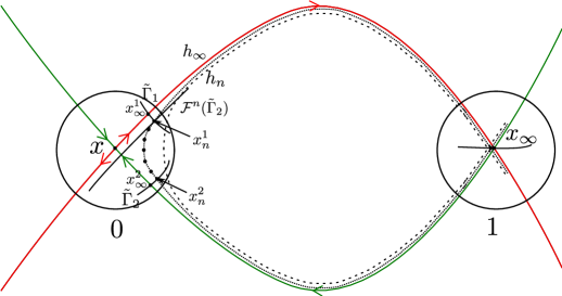
Figure 1. Selection of the periodic orbits $h_{n}$.

After going to a chart, we endow $\mathcal{S}_{0}$ with local coordinates. We denote by $x_{\infty}^{1}$, resp. $x_{\infty}^{2}$, the coordinates of the point of $h_{\infty}$ in $\mathcal{S}_{0}$ encoded by the symbolic sequence

$$x_{\infty}^{1}\,\longleftrightarrow\,\dots 000\underset{\begin{subarray}{c}\uparrow\end{subarray}}{0}10000\dots,\quad\text{resp. }x_{\infty}^{2}\,\longleftrightarrow\,\dots 00001\underset{\begin{subarray}{c}\uparrow\end{subarray}}{0}000\dots$$

Similarly, for any integer $n\geq 0$, we denote by $x_{n}^{1}$, resp. $x_{n}^{2}$, the coordinates of its periodic approximation in $h_{n}$, encoded by the symbolic sequence

$$x_{n}^{1}\,\longleftrightarrow\,\dots|0\dots 0\underset{\begin{subarray}{c}\uparrow\end{subarray}}{0}1|0\dots 01|\dots,\quad\text{resp. }x_{n}^{2}\,\longleftrightarrow\,\dots|0\dots 01|\underset{\begin{subarray}{c}\uparrow\end{subarray}}{0}0\dots 01|\dots$$

Note that the points $x_{\infty}^{1},x_{n}^{1}$, resp. $x_{\infty}^{2},x_{n}^{2}$ share the same symbolic past and future for $n$ steps, hence by hyperbolicity, they are exponentially close in phase space for $n\gg 1$ large. See Figure 1 for an illustration.

The point $x$ is a saddle fixed point under $\mathcal{F}$, with eigenvalues $0<\lambda<1<\lambda^{-1}$. The restriction of $\mathcal{F}$ to $\mathcal{S}_{0}$ is a local volume-preserving diffeomorphism. As recalled in Subsection 2.3, if $\mathcal{S}_{0}$ is chosen sufficiently small, then there exists a $C^{k}$ change of coordinates $R\colon\mathcal{S}_{0}\to{\mathbb{R}}^{2}$ under which $\mathcal{F}$ takes the form

$$N=N_{\Delta}\colon(\xi,\eta)\mapsto(\Delta(\xi\eta)\xi,\Delta(\xi\eta)^{-1}\eta),$$

for some $C^{k}$ function $\Delta\colon{\mathbb{R}}\to{\mathbb{R}}$ such that $\Delta(z)=\lambda+a_{1}z+o(z)$ for $|z|\ll 1$, where $a_{1}=a_{1}(\mathcal{O})$ is the first Birkhoff invariant at $\mathcal{O}$ of $\mathcal{F}$. For $k=\infty$, $\Delta$ is $C^{\infty}$, and $N$ is the Birkhoff Normal Form of $\mathcal{F}$.

For simplicity, in the following, we only detail the case where $k=\infty$, but the case of finite regularity $k\geq 5$ is handled similarly.

Lemma 3.2.

The conjugacy $R$ can be chosen in such a way that for all $n\gg 1$,

$$R(x_{n}^{1})=(\eta_{n},\xi_{n})\in\Gamma_{1},\qquad R(x_{n}^{2})=(\xi_{n},\eta_{n})\in\Gamma_{2},$$

where $\Gamma_{1},\Gamma_{2}$ are two smooth arcs which are mirror images of each other under the reflection with respect to the first bissectrix $\{\xi=\eta\}$.

Proof.

Let $\tilde{R}$ be any $C^{\infty}$ volume-preserving map such that $N=\tilde{R}\circ\mathcal{F}\circ(\tilde{R})^{-1}$. Inside $\mathcal{S}_{0}$, we have a foliation $\mathscr{H}$ by curves along which the motion happens, which corresponds to the preimage of the foliation by the hyperbolas $\{\xi\eta=\mathrm{cst}\}$ under $\tilde{R}$. Let us consider the square of the Poincaré map $\mathcal{F}$ restricted to a small neighbourhood $\mathcal{S}_{\infty}^{1}\subset\mathcal{S}_{0}$ of $x_{\infty}^{1}$. It follows from the definition of $x_{\infty}^{1},x_{\infty}^{2}$ that $\mathcal{F}^{2}$ maps $\mathcal{S}_{\infty}^{1}\subset\mathcal{S}_{0}$ to a small neighbourhood $\mathcal{S}_{\infty}^{2}\subset\mathcal{S}_{0}$ of $x_{\infty}^{2}$. The leaf of $\mathscr{H}$ through $x_{\infty}^{1}$ coincides with the local unstable leaf $\mathcal{W}_{\mathcal{F},\mathrm{loc}}^{u}(x_{\infty}^{1})\subset\mathcal{W}_{\mathcal{F}}^{u}(x)$, while the leaf of $\mathscr{H}$ through $x_{\infty}^{2}$ coincides with the local stable leaf $\mathcal{W}_{\mathcal{F},\mathrm{loc}}^{s}(x_{\infty}^{2})\subset\mathcal{W}_{\mathcal{F}}^{s}(x)$. In particular, locally, the leaves of the foliation $\mathscr{H}\cap\mathcal{S}_{\infty}^{1}$ are close to the unstable leaf $\mathcal{W}_{\mathcal{F},\mathrm{loc}}^{u}(x_{\infty}^{1})$, while the leaves of $\mathscr{H}\cap\mathcal{S}_{\infty}^{2}$ are close to the stable leaf $\mathcal{W}_{\mathcal{F},\mathrm{loc}}^{s}(x_{\infty}^{2})$. Besides, due to the presence of the homoclinic intersection between $\mathcal{W}_{\mathcal{F}}^{u}(x)$ and $\mathcal{W}_{\mathcal{F}}^{s}(x)$, the image under $\mathcal{F}^{2}$ of $\mathcal{W}_{\mathcal{F},\mathrm{loc}}^{u}(x_{\infty}^{1})$ intersects $\mathcal{W}_{\mathcal{F},\mathrm{loc}}^{s}(x_{\infty}^{2})$ transversally. We conclude that the foliation $\mathcal{F}^{2}(\mathscr{H}\cap\mathcal{S}_{\infty}^{1})=\{\mathcal{F}^{2}(\mathscr{H}_{t}^{1})\}_{t}$ is transverse to the foliation $\mathscr{H}\cap\mathcal{S}_{\infty}^{2}=\{\mathscr{H}_{t}^{2}\}_{t}$ provided that $\mathcal{S}_{\infty}^{1},\mathcal{S}_{\infty}^{2}$ are chosen sufficiently small, where for $|t|\ll 1$, $\mathscr{H}_{t}^{1}$ denotes the leaf of the foliation $\mathscr{H}\cap\mathcal{S}_{\infty}^{1}$ coming from the hyperbola $\{\xi\eta=t\}$, and $\mathscr{H}_{t}^{2}$ denotes the leaf of the foliation $\mathscr{H}\cap\mathcal{S}_{\infty}^{2}$ coming from the same hyperbola $\{\xi\eta=t\}$. Since the foliation $\mathscr{H}$ is smooth (it is the image under $\tilde{R}$ of the foliation $\{\xi\eta=\mathrm{cst}\}$), the locus of intersection $\{\mathcal{F}^{2}(\mathscr{H}_{t}^{1})\cap\mathscr{H}_{t}^{2}\}_{|t|\ll 1}$ is a $C^{\infty}$ curve $\tilde{\Gamma}_{2}$ containing the point $x_{\infty}^{2}$. Similarly, we denote by $\tilde{\Gamma}_{1}$ the locus of intersection of $\mathcal{F}^{-2}(\mathscr{H}_{t}^{2})$ and $\mathscr{H}_{t}^{1}$ near the point $x_{\infty}^{1}$ (see Figure 1).

Let us denote by $\hat{\Gamma}_{1}$ and $\hat{\Gamma}_{2}$ the respective images of the arcs $\tilde{\Gamma}_{1}$ and $\tilde{\Gamma}_{2}$ under $\tilde{R}$. For any $C^{\infty}$ function $D$, the map $N_{D}\colon(\xi,\eta)\mapsto(D(\xi\eta)\cdot\xi,D(\xi\eta)^{-1}\cdot\eta)$ commutes with $N$, hence $N_{D}\circ\tilde{R}$ also conjugates $\mathcal{F}$ with its Birkhoff Normal Form. By replacing $\tilde{R}$ with $N_{D}\circ\tilde{R}$ for some suitable function $D$, without loss of generality, we may assume that locally, $\hat{\Gamma}_{1}=\{(\xi,\hat{\gamma}_{1}(\xi))\}_{\xi}$, resp. $\hat{\Gamma}_{2}=\{(\xi,\hat{\gamma}_{2}(\xi))\}_{\xi}$, is a graph near $\tilde{R}(x_{\infty}^{1})=:(0,\tilde{\xi}_{\infty}^{1})$, resp. $\tilde{R}(x_{\infty}^{2})=:(\tilde{\xi}_{\infty}^{2},0)$. Let us look for $D$ such that $N_{D}(\hat{\Gamma}_{1})=\{(D(\xi\hat{\gamma}_{1}(\xi))\xi,D(\xi\hat{\gamma}_{1}(\xi))^{-1}\hat{\gamma}_{1}(\xi))\}_{\xi}$ and $N_{D}(\hat{\Gamma}_{2})=\{(D(\xi\hat{\gamma}_{2}(\xi))\xi,D(\xi\hat{\gamma}_{2}(\xi))^{-1}\hat{\gamma}_{2}(\xi))\}_{\xi}$ are mirror images of each other under the involution $\mathcal{I}_{0}\colon(\xi,\eta)\mapsto(\eta,\xi)$. As the latter preserves hyperbolas $\{\xi\eta=\mathrm{cst}\}$, this happens if and only if

$$D(\xi\hat{\gamma}_{1}(\xi))^{-1}\hat{\gamma}_{1}(\xi)=D(\hat{\xi}\hat{\gamma}_{2}(\hat{\xi}))\hat{\xi},$$

where $\hat{\xi}=\hat{\xi}(\xi)$ is the unique number such that $\hat{\xi}\hat{\gamma}_{2}(\hat{\xi})=\xi\hat{\gamma}_{1}(\xi)$. Note that for $|\xi|$ small, i.e., for $(\xi,\hat{\gamma}_{1}(\xi))$ close to $\tilde{R}(x^{1}_{\infty})=(0,\tilde{\xi}_{\infty}^{1})$, the existence of $\hat{\xi}(\xi)$ is guaranteed by the implicit function theorem. Indeed, by the transverse intersection between the stable and the unstable manifolds at $x_{\infty}^{2}$, we have $\hat{\gamma}_{2}^{\prime}(\tilde{\xi}_{\infty}^{2})\neq 0$; moreover, the map $\xi\mapsto\hat{\xi}(\xi)$ is smooth. The previous equation thus yields

$$D(\xi\hat{\gamma}_{1}(\xi))=\sqrt{\frac{\hat{\gamma}_{1}(\xi)}{\hat{\xi}(\xi)}}.$$

As $\lim_{\xi\to 0}\hat{\gamma}_{1}(\xi)=\tilde{\xi}_{\infty}^{1}\neq 0$ and $\lim_{\xi\to 0}\hat{\xi}(\xi)=\tilde{\xi}_{\infty}^{2}\neq 0$, and since $\hat{\gamma}_{1}^{\prime}(0)\neq 0$, the function $\xi\mapsto D(\xi)$ it defines is smooth near $0$, and the associated change of coordinates $R:=N_{D}\circ\tilde{R}$ satisfies the desired conditions.

Figure 2. Periodic orbits in Birkhoff coordinates.

Let $\Gamma_{1}$ and $\Gamma_{2}$ be the respective images of $\tilde{\Gamma}_{1}$ and $\tilde{\Gamma}_{2}$ under $R$. Note that for any large integer $n\gg 1$, the periodic orbit $h_{n}$ has “cyclicity” one, hence the points $x_{n}^{1},x_{n}^{2}\in h_{n}$ belong to the same curve $R^{-1}(\{\xi\eta=t_{n}\})$, for some $t_{n}\in{\mathbb{R}}$. Thus,

$$(\xi_{n},\eta_{n}):=R(x_{n}^{2})=R(\mathcal{F}^{2}(x_{n}^{1}))\in R\big{(}\mathcal{F}^{2}(\mathscr{H}_{t_{n}}^{1})\cap\mathscr{H}_{t_{n}}^{2}\big{)}=\Gamma_{2}.$$

Similarly, $R(x_{n}^{1})\in\Gamma_{1}$. As $\Gamma_{1},\Gamma_{2}$ are mirror images of each other under $(\xi,\eta)\mapsto(\eta,\xi)$, and $R(x_{n}^{1}),R(x_{n}^{2})\in\{\xi\eta=t_{n}\}$, with $t_{n}=\xi_{n}\eta_{n}$, we have $R(x_{n}^{1})=(\eta_{n},\xi_{n})$. ∎

In the following, we fix a conjugacy map $R$ as given by Lemma 3.2. We denote by $\mathcal{W}^{1}_{\infty}\subset R(\mathcal{S}_{\infty}^{1})$ the arc of the stable manifold through $R(x_{\infty}^{1})=:(0,\xi_{\infty})$, and we let $\mathcal{W}^{2}_{\infty}\subset R(\mathcal{S}_{\infty}^{2})$ be the arc of the unstable manifold through $R(x_{\infty}^{2})=:(\xi_{\infty},0)$. See Figure 2 for an illustration.

Lemma 3.3.

The arcs $\Gamma_{1}$, $\mathcal{W}^{1}_{\infty}$ and $\{(0,\xi_{\infty}+\eta):|\eta|\ll 1\}$ are pairwise transverse at $(0,\xi_{\infty})$.

Proof.

The last two arcs are transverse because they are pieces respectively of the stable and of the unstable manifold of the origin. In the following, we assume that $\Gamma_{1}=\{(\eta,\gamma(\eta)):|\eta|\ll 1\}$ is the graph of some smooth function $\gamma$ and show that it is transverse to $\mathcal{W}^{1}_{\infty}$ at $(0,\xi_{\infty})$. The other case is handled similarly.

We use the same notation as in Lemma 3.2. Recall that the arc $\Gamma_{1}$ is the locus of intersection of $\{R\circ\mathcal{F}^{-2}(\mathscr{H}_{t}^{2})\}_{t}$ and $\{R(\mathscr{H}_{t}^{1})\}_{t}$. Without loss of generality, after going to some chart, we may assume that for $|t|$ small, the foliations $\{R\circ\mathcal{F}^{-2}(\mathscr{H}_{t}^{2})\}_{t}$ and $\{R(\mathscr{H}_{t}^{1})\}_{t}$ are given by

$$R(\mathscr{H}_{t}^{1}) =\{\eta=t\},$$

$$R\circ\mathcal{F}^{-2}(\mathscr{H}_{t}^{2}) =\{(\eta,f(t,\eta)):|\eta|\ll 1\},$$

for some smooth function $f(\cdot,\cdot)$, so that $\gamma(\eta)=f(\eta,\eta)$, for $|\eta|$ small. On the one hand, the arc $\mathcal{W}_{\infty}^{1}$ coincides with the leaf $R\circ\mathcal{F}^{-2}(\mathscr{H}_{0}^{2})=\{(\eta,f(0,\eta)):|\eta|\ll 1\}$, whose tangent space at $(0,\xi_{\infty})$ is equal to

(3.2) $$\mathrm{Span}(1,\partial_{2}f(0,0)).$$

On the other hand, the tangent space to $\Gamma_{1}=\{(\eta,f(\eta,\eta)):|\eta|\ll 1\}$ at $(0,\xi_{\infty})$ is equal to

$$\mathrm{Span}(1,\partial_{1}f(0,0)+\partial_{2}f(0,0)).$$

As $\partial_{1}f(0,0)\neq 0$, we conclude that $\mathcal{W}^{1}_{\infty}$ and $\Gamma_{1}$ are transverse at $(0,\xi_{\infty})$. ∎

In the following, we denote by $\gamma_{0}+\gamma_{1}\eta+\gamma_{2}\eta^{2}+\dots$ the Taylor expansion at $0$ of the smooth function $\gamma$ whose graph is equal to $\Gamma_{1}=\{(\eta,\gamma(\eta)):|\eta|\ll 1\}$. Note that $\gamma_{0}=\xi_{\infty}$. Moreover, for any integer $n\geq 0$, we abbreviate $x_{n}^{1}=x_{n}$, and we denote by $\mathcal{L}_{n}=\mathcal{L}(x_{n})>0$ the period of $x_{n}$ for $\Phi$. We also denote by $\mathcal{L}^{(0)}=\mathcal{L}(x)>0$ the period of $x$, and we set $\lambda:=e^{-h_{\mathrm{top}}(\Phi)\mathcal{L}^{(0)}}\in(0,1)$.

Lemma 3.4.

We have the following asymptotic expansion for the periods $(\mathcal{L}_{n})_{n\geq 0}$:

$$\mathcal{L}_{n}=n\mathcal{L}^{(0)}+\mathcal{L}^{(1)}+O(\lambda^{n}),$$

for some constant $\mathcal{L}^{(1)}\in{\mathbb{R}}$.

Proof.

We refer the reader to [FMT, Lemma 4.2] for a detailed proof. Similar estimates in the case of dispersing billiards can also be found in [BDKL, Section 4].

Let us outline some of the steps of the proof. The computations are carried out by linearizing the dynamics in a neighbourhood of the saddle fixed point $x$. More precisely, we consider a cross section $\mathcal{S}$ as before and endow it with local coordinates near $x\in\mathcal{S}$. We denote by $\mathcal{F}$ the Poincaré map induced by the flow $\Phi$ on $\mathcal{S}$, and by $\tau\colon\mathcal{S}\to{\mathbb{R}}_{+}$ the first return time on $\mathcal{S}$. For any $\varepsilon>0$, there exist (see e.g. [Stow, ZZ]) a neighbourhood $\mathcal{U}\subset{\mathbb{R}}^{2}$ of $x\simeq(0,0)$, a neighbourhood $\mathcal{V}\subset{\mathbb{R}}^{2}$ of $(0,0)$, a linear isomorphism $P\in\mathrm{SL}(2,{\mathbb{R}})$, and a $C^{1,\frac{1}{2}}$-diffeomorphism $\Psi\colon\mathcal{U}\to\mathcal{V}$, such that

$$\Psi\circ\mathcal{F}\circ\Psi^{-1}=D_{\lambda},\qquad\|\Psi-P\|_{C^{1}}\leq\varepsilon,\qquad\|\Psi^{-1}-P^{-1}\|_{C^{1}}\leq\varepsilon,$$

with $D_{\lambda}:=\mathrm{diag}(\lambda,\lambda^{-1})\colon(\xi,\eta)\mapsto(\lambda\xi,\lambda^{-1}\eta)$, and

$$\Psi(z)-\Psi(z^{\prime}) =P(z-z^{\prime})+O(\max(|z|^{\frac{1}{2}},|z^{\prime}|^{\frac{1}{2}})|z-z^{\prime}|),$$

$$\Psi^{-1}(z)-\Psi^{-1}(z^{\prime}) =P^{-1}(z-z^{\prime})+O(\max(|z|^{\frac{1}{2}},|z^{\prime}|^{\frac{1}{2}})|z-z^{\prime}|).$$

As $n\to+\infty$, the points in the orbit $h_{n}$ get closer and closer to those in $h_{\infty}$. Since the orbit $h_{\infty}$ is homoclinic to $\mathcal{O}$, for $k\in{\mathbb{Z}}$, the first return time $\tau(\mathcal{F}^{k}(x_{\infty}^{1}))$ is exponentially close to $\mathcal{L}^{(0)}=\mathcal{L}(x)$ with respect to $|k|$. The total error $\mathcal{L}^{(1)}$ is obtained by adding up the discrepancies $\delta_{k}:=\tau(\mathcal{F}^{k}(x_{\infty}^{1}))-\mathcal{L}^{(0)}$ over all the points $(\mathcal{F}^{k}(x_{\infty}))_{k\in{\mathbb{Z}}}$. Thus, $\mathcal{L}_{n}-n\mathcal{L}^{(0)}-\mathcal{L}^{(1)}$ is the sum of two terms:

1. the sum $\sum_{k=-\lceil n/2\rceil}^{n+1-\lceil n/2\rceil}\tau(\mathcal{F}^{k}(x_{n}^{1}))-\tau(\mathcal{F}^{k}(x_{\infty}^{1}))$;

2. the tail $\sum_{\begin{subarray}{c}k>n+1-\lceil n/2\rceil\\ \text{or }k<-\lceil n/2\rceil\end{subarray}}\mathcal{L}^{(0)}-\tau(\mathcal{F}^{k}(x_{\infty}^{1}))$ of the series $-\sum_{k}\delta_{k}$.

In order to evaluate the first of these two terms, we need to estimate the coordinates of the points $\mathcal{F}^{k}(x_{n}^{1})$, for $k=-\lceil n/2\rceil,\dots,n+1-\lceil n/2\rceil$. Except a finite number $N\geq 0$ of them (uniform with respect to $n\geq 0$), all of these points are in the neighbourhood $\mathcal{U}$ where $\Psi$ is defined. In particular, there exist $y_{\infty}^{+},y_{\infty}^{-}\in\mathcal{V}\cap\Psi(h_{\infty})$ such that for all $n\gg 1$, there exists a point $y_{n}^{+}\in\mathcal{V}\cap\Psi(h_{n})$ whose iterates $y_{n}^{+},D_{\lambda}(y_{n}^{+}),\dots,y_{n}^{-}:=D_{\lambda}^{n+1-N}(y_{n}^{+})$ are all in $\mathcal{V}$ and such that $\lim_{n\to+\infty}y_{n}^{*}=y_{\infty}^{*}$, for $*=+,-$ (see Figure 3). By applying $\Psi^{-1}$, this allows us to estimate the difference $\tau(\mathcal{F}^{k}(x_{n}^{1}))-\tau(\mathcal{F}^{k}(x_{\infty}^{1}))$, for all $k=-\lceil n/2\rceil,\dots,n+1-\lceil n/2\rceil$. ∎

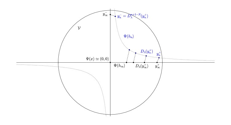
Figure 3. Linearization of the dynamics in a neighbourhood of $x\simeq(0,0)$.

The result of Proposition 3.1 can be reformulated as follows:

Lemma 3.5.

If the SRB measure is equal to the MME, then for each $n\geq 0$, the Floquet multipliers of $D\Phi_{x_{n}}^{\mathcal{L}_{n}}$ are equal to $e^{\pm h_{\mathrm{top}}(\Phi)\mathcal{L}_{n}}$.

Corollary 3.6.

If the SRB measure is equal to the MME, then as $n\to+\infty$, we get the asymptotic expansion

$$e^{\pm h_{\mathrm{top}}(\Phi)\mathcal{L}_{n}}=C_{\infty}^{\pm 1}\lambda^{\pm n}(1+O(\lambda^{n})),$$

where $C_{\infty}:=e^{h_{\mathrm{top}}(\Phi)\mathcal{L}^{(1)}}>0$.

In particular, as $\mathrm{tr}(D\mathcal{F}_{x_{n}}^{n+2})=\mathrm{tr}(D\Phi_{x_{n}}^{\mathcal{L}_{n}})-1=e^{-h_{\mathrm{top}}(\Phi)\mathcal{L}_{n}}+e^{h_{\mathrm{top}}(\Phi)\mathcal{L}_{n}}$, it holds

(3.3) $$2\cosh(\mathcal{L}_{n}\mathrm{LE}(h_{n}))=2\cosh(\mathcal{L}_{n}h_{\mathrm{top}}(\Phi))=C_{\infty}^{-1}\lambda^{-n}+O(1).$$

On the other hand, we can obtain a general expression for the Lyapunov exponents of the orbits $(h_{n})_{n\geq 0}$, which holds without any assumption on the MME with respect to the SRB measure. Let us recall that for each large integer $n\gg 1$, we denote by $(\xi_{n},\eta_{n})$ the coordinates of the point $R(x_{n}^{2})$ on $\Gamma_{2}$. By Lemma 3.2, and since $N^{n}(\xi_{n},\eta_{n})=N^{n}\circ R(x_{n}^{2})=R(x_{n}^{1})=(\eta_{n},\xi_{n})$, the pair $(\xi_{n},\eta_{n})$ is defined implicitely by the following system of equations:

$$\left\{\begin{array}[]{rcl}\xi_{n}&=&\gamma(\eta_{n}),\\ \eta_{n}&=&\Delta(\xi_{n}\eta_{n})^{n}\xi_{n}=\Delta(\gamma(\eta_{n})\eta_{n})^{n}\gamma(\eta_{n}).\end{array}\right.$$

In particular, this implies:

(3.4) $$\xi_{n}=\xi_{\infty}+O(\lambda^{n}),\quad\eta_{n}=\xi_{\infty}\lambda^{n}+O(n\lambda^{2n}).$$

Following the computations in [DKL, Lemma 4.10], we obtain:

Lemma 3.7.

As $n\to+\infty$, we have the asymptotic expansion

(3.5) $$2\cosh(\mathcal{L}_{n}\mathrm{LE}(h_{n}))=\mathrm{tr}(D\mathcal{F}_{x_{n}}^{n+2})=C_{0}\lambda^{-n}+nC_{1}a_{1}+O(1),$$

where $C_{0},C_{1}\in{\mathbb{R}}^{*}$ are nonzero constants, and $a_{1}\in{\mathbb{R}}$ is the first Birkhoff invariant at $\mathcal{O}$ of $\mathcal{F}$.

Proof.

Note that when the integer $n\gg 1$ gets large, the orbit $h_{n}$ shadows the homoclinic orbit $h_{\infty}$ very closely. Thus, as in [DKL], we can replace the dynamics of $\mathcal{F}$ near $h_{\infty}$ with that of the Birkhoff Normal Form $N$ and some gluing map $\mathcal{G}=R\circ\mathcal{F}^{2}\circ R^{-1}\colon O_{\infty}^{1}\to R(\mathcal{S}_{\infty}^{2})$ defined on an open subset $\{(0,\xi_{\infty})\}\in O_{\infty}^{1}\subset R(\mathcal{S}_{\infty}^{1})$. In particular, as the trace $\mathrm{tr}(D\mathcal{F}_{x_{n}}^{n+2})$ is invariant under the change of coordinates $R$, for any large integer $n\gg 1$, we get

$$\mathrm{tr}(D\mathcal{F}_{x_{n}}^{n+2})=\mathrm{tr}(D(N^{n}\circ\mathcal{G})_{(\eta_{n},\xi_{n})})=\mathrm{tr}(DN^{n}_{(\xi_{n},\eta_{n})}D\mathcal{G}_{(\eta_{n},\xi_{n})}).$$

Moreover, we have

$$DN^{n}_{(\xi,\eta)}=\begin{bmatrix}\Delta(\xi\eta)^{n}+n\Delta^{\prime}(\xi\eta)\Delta(\xi\eta)^{n-1}\xi\eta&n\Delta^{\prime}(\xi\eta)\Delta(\xi\eta)^{n-1}\xi^{2}\\ -n\Delta^{\prime}(\xi\eta)\Delta(\xi\eta)^{-n-1}\eta^{2}&\Delta(\xi\eta)^{-n}-n\Delta^{\prime}(\xi\eta)\Delta(\xi\eta)^{-n-1}\xi\eta\end{bmatrix}.$$

By (3.4), $\xi_{n}\eta_{n}=\xi_{\infty}^{2}\lambda^{n}+O(n\lambda^{2n})$; besides, $\Delta(\xi_{n}\eta_{n})=\lambda+a_{1}\xi_{\infty}^{2}\lambda^{n}+O(n\lambda^{2n})$, and $\Delta^{\prime}(\xi_{n}\eta_{n})=a_{1}+O(\lambda^{n})$, hence

$$DN_{(\xi_{n},\eta_{n})}^{n}=\begin{bmatrix}\lambda^{n}&0\\ 0&\lambda^{-n}\end{bmatrix}-\lambda^{-1}\xi_{\infty}^{2}a_{1}n\begin{bmatrix}-2\lambda^{2n}+O(n\lambda^{3n})&-\lambda^{n}+O(n\lambda^{2n})\\ \lambda^{n}+O(n\lambda^{2n})&2+O(n\lambda^{n})\end{bmatrix}.$$

Moreover, for $\gamma_{1}=\gamma^{\prime}(0)$, and some $g_{0}\in{\mathbb{R}}$, it holds: (see formula (4.4) in [DKL])

$$D\mathcal{G}_{(\eta_{n},\xi_{n})}=D\mathcal{G}_{(0,\xi_{\infty})}+O(\lambda^{n})=\begin{bmatrix}\gamma_{1}(2-\gamma_{1}g_{0})&\gamma_{1}g_{0}-1\\ 1-\gamma_{1}g_{0}&g_{0}\end{bmatrix}+O(\lambda^{n}).$$

We deduce that

$$\mathrm{tr}(D\mathcal{F}_{x_{n}}^{n+2}) =\mathrm{tr}\bigg{(}\begin{bmatrix}0&0\\ 0&\lambda^{-n}-2\lambda^{-1}\xi_{\infty}^{2}a_{1}n\end{bmatrix}\begin{bmatrix}\gamma_{1}(2-\gamma_{1}g_{0})&\gamma_{1}g_{0}-1\\ 1-\gamma_{1}g_{0}&g_{0}\end{bmatrix}\bigg{)}+O(1)$$

$$=g_{0}\lambda^{-n}-2\lambda^{-1}\xi_{\infty}^{2}g_{0}a_{1}n+O(1).$$

In particular, the constants $C_{0},C_{1}\in{\mathbb{R}}$ in (3.5) are given by

$$C_{0}:=g_{0},\quad C_{1}:=-2\lambda^{-1}\xi_{\infty}^{2}g_{0}.$$

Since the gluing map $\mathcal{G}$ is dynamically defined, the vector $(1,w_{1})$ tangent to $\mathcal{W}_{\infty}^{1}$ at $(0,\xi_{\infty})$ is mapped to a vector $(*,1-g_{0}(\gamma_{1}-w_{1}))$ in the stable subspace at $(\xi_{\infty},0)$, which is horizontal in our coordinate system. We deduce that $g_{0}(\gamma_{1}-w_{1})=1$, and by Lemma 3.3, $w_{1}\neq\gamma_{1}\neq\infty$, so that

(3.6) $$g_{0}=(\gamma_{1}-w_{1})^{-1}\neq 0,$$

hence $C_{0},C_{1}\neq 0$ (note that $\xi_{\infty}\neq 0$). ∎

Corollary 3.8.

If the SRB measure is equal to the MME, then for any periodic orbit $\mathcal{O}$, the first Birkhoff invariant at $\mathcal{O}$ of the Poincaré map $\mathcal{F}$ vanishes.

Proof.

We consider the periodic point $x$ as above and use the notation introduced previously. By equating the expressions obtained in (3.3) and (3.5), for $n\gg 1$, we obtain

$$2\cosh(\mathcal{L}_{n}\mathrm{LE}(h_{n}))=C_{\infty}^{-1}\lambda^{-n}+O(1)=C_{0}\lambda^{-n}+nC_{1}a_{1}+O(1).$$

Since $C_{1}\neq 0$, we deduce that $a_{1}=0$, as desired. ∎

By Theorem 2.17, we deduce:

Corollary 3.9.

If the SRB measure is equal to the MME, then the Anosov class $[A_{\Phi}]$ vanishes.

Gathering the previous observations, we thus obtain:

Corollary 3.10.

Let $k\geq 5$ be some integer, and let $\Phi$ be a volume-preserving $C^{k}$ Anosov flow on some $3$-dimensional compact connected manifold $M$.

1. If the MME of $\Phi$ is equal to the volume measure, then the weak stable/unstable distributions $E_{\Phi}^{cs}/E_{\Phi}^{cu}$ are $C^{k-3}$.

2. If the MME of $\Phi$ is equal to the volume measure, then $\Phi$ is $C^{k}$-orbit equivalent to an algebraic flow.

3. If $\Phi$ is obtained by suspending an Anosov diffeomorphism $F$ of the $2$-torus ${\mathbb{T}}^{2}$, then the MME of $\Phi$ is equal to the volume measure if and only if $F$ is $C^{k-3}$ conjugate to a linear automorphism.

Proof.

Item 1, resp. 3, follows from Corollary 3.9 and Theorem 2.17 (Theorem 3.4/Corollary 3.5 in [HuKa]), resp. Corollary 3.6 of Hurder-Katok [HuKa]. Besides, Item 2 follows from Item 1 and Theorem 2.18 (Théorème 4.6 in Ghys [G2]). ∎

3.3. From smooth orbit equivalence to smooth flow conjugacy

In this subsection, as in Corollary 3.10, let $k\geq 5$, and let $\Phi$ be a $C^{k}$ Anosov flow on some $3$-dimensional manifold $M$ which preserves a smooth volume $\mu$.

The following result explains how we can upgrade the smooth equivalence obtained in Corollary 3.10 to a smooth flow conjugacy.

Proposition 3.11.

If the MME of $\Phi$ is equal to the volume measure $\mu$, then for any $\varepsilon>0$, $\Phi$ is $C^{k-\varepsilon}$ conjugate to an algebraic flow.

Proof.

Since the MME is equal to the volume measure $\mu$, by Corollary 3.10, we know that $\mathcal{W}^{cs}_{\Phi}$ and $\mathcal{W}^{cu}_{\Phi}$ are $C^{k-3}$ foliations, and the flow $\Phi$ is orbit equivalent to an algebraic flow $\Psi$ through a $C^{k}$ map $\mathcal{H}$. Up to a linear time change, without loss of generality, we can assume that the topological entropies of $\Phi,\Psi$ coincide, i.e. $h_{\mathrm{top}}(\Phi)=h_{\mathrm{top}}(\Psi)=h>0$. Moreover, up to a $C^{k}$ conjugacy, the flow $\Phi$ can be seen as a reparametrization of the algebraic flow $\Psi$.

Let $x\in M$ be a point in some periodic orbit $\mathcal{O}$ of $\Phi$, of period $\mathcal{L}_{\Phi}(\mathcal{O})=\mathcal{L}_{\Phi}(x)>0$. The orbit $\mathcal{O}$ is also periodic for $\Psi$, of period $\mathcal{L}_{\Psi}(\mathcal{O})=\mathcal{L}_{\Psi}(x)>0$. As the MME is equal to the volume measure $\mu$, Proposition 3.1 yields

(3.7) $$J_{\Phi,x}^{u}(\mathcal{L}_{\Phi}(x))=e^{h\mathcal{L}_{\Phi}(x)},$$

where $J_{\Phi,x}^{u}(\mathcal{L}_{\Phi}(x))>1$ is the unstable Jacobian of $\Phi$ at $x$.

Similarly, for the algebraic flow $\Psi$, we have

(3.8) $$J_{\Psi,x}^{u}(\mathcal{L}_{\Psi}(x))=e^{h\mathcal{L}_{\Psi}(x)}.$$

Let us take a smooth section $\mathcal{S}_{x}$ transverse to the flows $\Phi,\Psi$ at $x$. As $\Phi$ is a smooth reparametrization of $\Psi$, the two flows induce the same Poincaré map on $\mathcal{S}_{x}$, which we denote by $\mathcal{F}$. When $\mathcal{F}$ is seen as the Poincaré map of $\Phi$, resp. $\Psi$, the eigenvalues of its differential $D\mathcal{F}_{x}$ (which are independent of the choice of the point $x$ and of the transverse section at $x$) are equal to $(J_{\Phi,x}^{u}(\mathcal{L}_{\Phi}(x)))^{\pm 1}$, resp. $(J_{\Psi,x}^{u}(\mathcal{L}_{\Psi}(x)))^{\pm 1}$, hence $J_{\Phi,x}^{u}(\mathcal{L}_{\Phi}(x))=J_{\Psi,x}^{u}(\mathcal{L}_{\Psi}(x))$. Together with (3.7) and (3.8), we conclude that for any periodic orbit $\mathcal{O}$, the associated periods for $\Phi$ and $\Psi$ are equal, i.e.,

(3.9) $$\mathcal{L}_{\Phi}(\mathcal{O})=\mathcal{L}_{\Psi}(\mathcal{O}).$$

Based on (3.9), we can produce a continuous flow conjugacy following a classical “synchronization” procedure, which we now recall.

Let us denote by $X_{\Phi}\cdot\mathcal{H}$ the derivative of $\mathcal{H}$ with respect to the flow vector field $X_{\Phi}$; then for any $x\in M$, it holds

$$X_{\Phi}\cdot\mathcal{H}(x)=w_{\mathcal{H}}(x)X_{\Psi}(\mathcal{H}(x)),$$

for some function $w_{\mathcal{H}}\colon M\to{\mathbb{R}}$ which measures the “speed” of $\mathcal{H}$ along the flow direction. By (3.9), the function $w_{\mathcal{H}}-1$ integrates to $0$ over all periodic orbits. By Livsic’s theorem (see [HaKa], Subsection 9.2), we deduce that there exists a continuous function $u\colon M\to{\mathbb{R}}$ differentiable along the direction of the flow $\Phi$ such that $w_{\mathcal{H}}-1=X_{\Phi}\cdot u$. Now, let $\mathcal{H}_{0}\colon x\mapsto\Psi^{-u(x)}\circ\mathcal{H}(x)$. Given any $x\in M$, we compute

$$w_{\mathcal{H}_{0}}(x)X_{\Psi}(\mathcal{H}_{0}(x)) =X_{\Phi}\cdot(\Psi^{-u(x)}\circ\mathcal{H})(x)$$

$$=\big{(}w_{\mathcal{H}}(x)-X_{\Phi}\cdot u(x)\big{)}X_{\Psi}(\Psi^{-u(x)}\circ\mathcal{H}(x))=X_{\Psi}(\mathcal{H}_{0}(x)),$$

i.e., $w_{\mathcal{H}_{0}}\equiv 1$. It follows that the homeomorphism $\mathcal{H}_{0}$ conjugates the flows $\Phi$ and $\Psi$:

$$\mathcal{H}_{0}\circ\Phi^{t}=\Psi^{t}\circ\mathcal{H}_{0},\quad\forall\,t\in{\mathbb{R}}.$$

Besides, the Lyapunov exponents of corresponding periodic orbits of $\Phi$ and $\Psi$ coincide (by Proposition 3.1, they are all equal to $h_{\mathrm{top}}(\Phi)=h_{\mathrm{top}}(\Psi)=h$). We conclude from a rigidity result of de la Llave (Theorem 1.1 in [dlL], see also [dlLM] where the $C^{\infty}$ case was considered) that the conjugacy $\mathcal{H}_{0}$ is in fact $C^{k-\varepsilon}$, for any $\varepsilon>0$. ∎

Let us now conclude the proof of Theorem A. Given $k\geq 5$ and a $C^{k}$ Anosov flow $\Phi$ on some three manifold preserving a smooth volume measure $\mu$, if the MME of $\Phi$ is equal to $\mu$, then Proposition 3.11 says that $\Phi$ is $C^{k-\varepsilon}$ conjugate to an algebraic flow, for any $\varepsilon>0$. Conversely, assume that $\Phi$ is a volume-preserving Anosov flow on some three manifold that is conjugate to an algebraic flow $\Psi$ through a smooth map $\mathcal{H}$. As the MME of $\Psi$ coincides with the SRB measure, and the smooth conjugacy $\mathcal{H}$ takes the MME, resp. the SRB of $\Phi$ to the MME, resp. the SRB of $\Psi$, we conclude that the MME of $\Phi$ coincides with the volume measure, as desired. ∎

4. Entropy Flexibility

Theorem A has shown that for an Anosov flow $\Phi$ on some $3$-manifold preserving a smooth volume $\mu$, $h_{\operatorname{top}}(\Phi)=h_{\mu}(\Phi)$ if and only if $\Phi$ is an algebraic flow up to smooth conjugacy. In particular, the topological entropy $h_{\operatorname{top}}(\Phi)$ and the measure-theoretic entropy $h_{\mu}(\Phi)$ for the volume measure have to be the same for algebraic flows. It is then natural to ask: what about non-algebraic flows? Here we show that the numbers of the topological entropy $h_{\operatorname{top}}(\Phi)$ and the measure-theoretic entropy $h_{\mu}(\Phi)$ with respect to the volume measure for the suspension flows over Anosov diffeomorphisms are quite flexible for non-algebraic flows.

We normalize the total volume of the suspension space to $1$ (equivalently, we normalize the integral of $r$ with respect to Lebesgue to be $1$), i.e., $\int r\,d\mu=1$. One may also think of this as finding a canonical linear time change of an arbitrary flow, and is analogous to fixing the volume of a surface when considering geodesic flows. There are three natural restrictions on $h_{\operatorname{top}}(\Phi)$ and $h_{\mu}(\Phi)$. The Pesin entropy formula and positivity of Lyapunov exponents imply that $h_{\mu}(\Phi)>0$. Moreover, the variational principle implies

$$h_{\operatorname{top}}(\Phi)\geq h_{\mu}(\Phi).$$

Finally, the Abramov formula gives

$$h_{\mu}(\Phi)=\frac{h_{\mu}(f)}{\int r\,d\mu}=h_{\mu}(f)\leq h_{\operatorname{top}}(f)=:h.$$

Here we denote by $h$ the topological entropy of the torus automorphism in the same homotopy class as $f$. Since any two Anosov diffeomorphisms in the same homotopy class are conjugated with each other [Fr], we have $h=h_{\operatorname{top}}(g)$, for any $g$ in the same homotopy class as $f$.

In this section, we shall prove Theorem D which says that the pair of values of entropy under the three natural restrictions mentioned above can all be achieved. Let $A\in\mathrm{SL}(2,{\mathbb{Z}})$ be a hyperbolic matrix whose induced torus automorphism has topological entropy $h$. Let $\mu$ be the volume measure on ${\mathbb{T}}^{2}$. Then for any $c_{\operatorname{top}}>c_{\mu}>0$ such that $c_{\mu}\leq h$, we shall find a volume-preserving Anosov diffeomorphism $f\colon{\mathbb{T}}^{2}\to{\mathbb{T}}^{2}$ homotopic to $A$ and a $C^{\infty}$ function $r\colon{\mathbb{T}}^{2}\to{\mathbb{R}}^{+}$ with integral $1$ with respect to the volume measure such that if $\Phi$ is the suspension flow induced by $f$ and $r$, then $h_{\operatorname{top}}(\Phi)=c_{\operatorname{top}}$ and $h_{\mu}(\Phi)=c_{\mu}$.

The figure to the right shows the content of Theorem D, where the horizontal axis is $h_{\mu}$ and the vertical axis is $h_{\mathrm{top}}$. The dashed area can be achieved by some suspension flow. The corner point represents the unique flow up to $C^{\infty}$ conjugacy, namely the algebraic flow. The boundaries are not achievable, with the exception of the right boundary. If we relax the regularity to $C^{1+\alpha}$ the bottom boundary is achievable.

To prove Theorem D, we shall use the following lemma, which follows immediately from the variational principle and Abramov formula.

Lemma 4.1 (Theorem 2 in [KKW]).

Suppose that $f\colon M\to M$ is an Anosov diffeomorphism of a smooth manifold, and $\Phi_{r}$ is the suspension flow of $f$ with $C^{\infty}$ roof function $r$. Then $r\mapsto h_{\operatorname{top}}(\Phi_{r})$ is continuous.

Proof of Theorem D.

We first realize the region II. By [HJJ] (see also [E]), for any $h\geq c_{\mu}>0$, there exists a volume-preserving Anosov map $f\colon{\mathbb{T}}^{2}\to{\mathbb{T}}^{2}$ of homotopy type $A$ such that $h_{\mu}(f)=c_{\mu}$. Taking the roof function $r\equiv 1$ gives the case where $c_{\operatorname{top}}=h$. Since we may homotope the roof function to a constant, it suffices to show that $h_{\operatorname{top}}(\Phi_{r})$ can be made arbitrarily large while keeping $\int r=1$, by Lemma 4.1. A similar approach also appeared in [EK]. Given $\varepsilon,\delta>0$, let $r\colon{\mathbb{R}}^{2}\to{\mathbb{R}}^{+}$ be a $C^{\infty}$ function satisfying $r\geq\delta$, $\int r\,d\mu=1$ and $r|_{{\mathbb{T}}^{2}\setminus B_{\varepsilon}(0)}\equiv\delta$. It is clear that such functions exist. Let $\sigma\colon\Sigma_{0}\to\Sigma_{0}$ be a Markov shift coding $f$, with coding map $\pi\colon\Sigma_{0}\to{\mathbb{T}}^{2}$. By choosing $\varepsilon$ sufficiently small, and a sufficient refinement of a Markov parition for $f$, we can find a subshift $\Sigma\subset\Sigma_{0}$ such that $\pi(\Sigma)\cap B_{\varepsilon}(0)=\emptyset$ and $h_{\operatorname{top}}(\sigma|_{\Sigma})>0$. This can be constructed easily symbolically by increasing the “memory” of $\Sigma_{0}$ and disallowing the blocks containing $0$, but a more geometric construction can be found in [K2, Corollary 4.3]. Hence the topological entropy of the flow is at least the topological entropy of the flow restricted to the suspension of this subshift. Since $r$ is identically $\delta$ on $\pi(\Sigma)$, $h_{\operatorname{top}}(\Phi_{r})\geq h_{\operatorname{top}}(\sigma|_{\Sigma})/\delta$. Since $\delta$ can be arbitrarily small, we get the result.

Now we consider the case where $c_{\mu}<c_{\operatorname{top}}<h$ (i.e., region I). We start by again taking an Anosov diffeomorphism $f\colon{\mathbb{T}}^{2}\to{\mathbb{T}}^{2}$ such that $h_{\mu}(f)=c_{\mu}$. If we choose the $C^{1+\alpha}$ roof function $x\mapsto\|Df_{x}|_{E^{u}_{f}}\|$ (normalized to have integral one), we obtain a flow such that $h_{\operatorname{top}}(\Phi_{r})=h_{\mu}(f)=c_{\mu}$. By perturbing $r$ to a $C^{\infty}$ roof function $C^{1}$-close to $r$ and the continuity of topological entropy, we can get a $C^{\infty}$ roof function with topological entropy arbitrarily close to $c_{\mu}$. Then taking a linear homotopy of the roof function to the constant one function gives all intermediate values. ∎

Another natural normalization for the roof function $r$ is to normalize its integral with respect to the measure of maximal entropy of the base. When normalizing with respect to the maximal entropy measure, the natural restrictions become $h_{\operatorname{top}}(\Phi)\geq h$ and $h_{\mu}(\Phi)\leq h_{\operatorname{top}}(\Phi)$. Theorem E tells us all of these numbers can be achieved.

The figure to the right shows the content of Theorem E, where the horizontal axis is $h_{\mu}$ and the vertical axis is $h_{\mathrm{top}}$. The dashed area can be achieved by some suspension flow. The corner point represents the unique flow up to $C^{\infty}$ conjugacy, namely the algebraic flow. The boundaries are not achievable, with the exception of the bottom boundary. If we relax the regularity to $C^{1+\alpha}$ the right boundary is achievable.

The proof of Theorem E is significantly more complicated. The reason is that we cannot change the value of topological entropy independently of the value of metric entropy with respect to the invariant volume. This was possible in Theorem D because the measure we normalized by was one of the measures being considered. Here, the MME for the base may not (and in most cases, will not) be the MME for the flow, so in reality, we must control three different measures on the base: the MME of the base, the invariant volume, and the measure which induces the MME of the flow. We shall use $\mu$ to refer to the volume measures and $\nu$ to indicate the corresponding maximal entropy measures. It is not surprising that we need the following lemma in the proof:

Lemma 4.2.

Fix any hyperbolic matrix $A\in\mathrm{SL}(2,{\mathbb{Z}})$, there exist $\Sigma$, a proper subshift of $A$, a Markov measure $\rho$ on $\Sigma$ with positive entropy such that for every $\delta>0$, $L>0$, there is a one-parameter family $\{f_{t}\}_{t\in[0,1]}$ of $C^{\infty}$, area-preserving Anosov diffeomorphisms continuous in the $C^{1}$ topology such that if $\pi_{t}\colon\Sigma\to{\mathbb{T}}^{2}$ is the continuously varying embedding of the subshift, then

1. $f_{0}$ is the hyperbolic toral automorphism induced by $A$;

2. $h_{\mu}(f_{1})<\delta$;

3. $\lambda_{\nu_{1}}(f_{1})>L$;

4. $\lambda_{(\pi_{1})_{*}\rho}(f_{1})<\delta$.

Proof.

Parts (i)-(iii) of the lemma are exactly the content of [E]. So we must find the subshift $\Sigma$ and measure $\rho$. By Franks-Manning [Fr], there exists a topological conjugacy between $A$ and $f_{t}$. We shall construct an embedding of subshift for $f_{1}$ and then $\Sigma$ for $f_{t}$ and moreover for $A$ will be obtained through the conjugacy. If $p$ is a periodic orbit of $A$, notice that there are associated periodic orbits of $f_{t}$ obtained through the Franks-Manning conjugacy. Let $\lambda_{p}(t)$ denote the multiplier of $p_{t}$ for $f_{t}$. We claim that there exists $p\in{\mathbb{T}}^{2}$ such that $\lambda_{p}(1)<\delta$. If this were not true, then the Lyapunov exponent of every periodic measure would converge to something at least $\delta$. Since Lebesgue measure is a Gibbs state, it can be arbitrarily well approximated by a periodic measure. This would imply that the exponent of Lebesgue measure is at least $\delta$, contradicting (ii).

Let $p$ be a periodic point such that $\lambda_{p}(1)<\delta$, and $q$ denote the period of $p$. We may without loss of generality assume that $\|D(f_{1}^{q})_{p}\|=e^{\delta^{\prime}}$, where $\delta^{\prime}<\delta$. Choose a Markov partition fine enough so that any cylinder set $C$ of length $q$ containing $p$ has $\|D(f_{1}^{q})_{x}\|<e^{2\delta^{\prime}}$ for all $x\in C$. Now, choose any Markov measure which gives the union of these cylinder sets measure $1-\frac{\delta^{\prime}}{\max\|Df_{1}\|}$, and any other cylinder set measure 0. Then the Lyapunov exponent is obtained by integrating the unstable Jacobian with respect to this measure, which will be smaller than $2\delta^{\prime}(1-\frac{\delta^{\prime}}{\max\|Df_{1}\|})+\frac{\delta^{\prime}}{\max\|Df_{1}\|}\cdot\max\|Df_{1}\|$, which is linear in $\delta^{\prime}$. Revising our choice of $\delta^{\prime}$ (to, e.g., $\delta/3$) gives the result. ∎

Lemma 4.3.

Let $\gamma>0$, $f\colon{\mathbb{T}}^{2}\to{\mathbb{T}}^{2}$ be any $C^{\infty}$ diffeomorphism not smoothly conjugate to its corresponding automorphism, and $\rho$ be an ergodic Markov measure supported on a subshift of finite type containing a fixed point $x_{0}$. Then there exists a positive $C^{\infty}$ function $q\colon{\mathbb{T}}^{2}\to{\mathbb{R}}$ such that:

• $\int q\,d\mu=1$;

• $\int q\,d\nu=1$, where $\nu$ is the measure of maximal entropy for $f$;

• $\int q\,d\rho=\gamma$.

Proof.

For convenience, we denote $\omega_{1}=\mu$, $\omega_{2}=\nu$ and $\omega_{3}=\rho$. Then the $\omega_{i}$ are linearly independent, since each $\omega_{i}$ is ergodic, $\mu$ and $\nu$ are both fully supported but singular since $f$ is not smoothly conjugate to an automorphism, and $\rho$ is supported on a Cantor set. By our assumptions, we may find some $g\colon{\mathbb{T}}^{2}\to{\mathbb{R}}$ continuous such that $g_{i}=\int g\,d\omega_{i}$ are all distinct. Let $\eta<\frac{1}{2}\min_{i\neq j}\{|g_{i}-g_{j}|\}$, and

$$U_{N,i}:=\left\{x\in{\mathbb{T}}^{2}:\left|\frac{1}{N}\sum_{k=0}^{N-1}g(f^{k}(x))-g_{i}\right|<\eta\right\}.$$

By choice of $\eta$, the $U_{N,i}$ are pairwise disjoint for every $N$. Furthermore, by the Birkhoff Ergodic theorem, $\omega_{i}(U_{N,i})\to 1$ as $N\to\infty$. Given $\alpha^{\prime}>0$, we may choose $N$ sufficiently large so that $\mu(U_{N,i})>1-\alpha^{\prime}$ (which, since $U_{N,i}\cap U_{N,j}=\emptyset$, implies that $\omega_{i}(U_{N,j})<\alpha^{\prime}$). Given $\alpha>0$, we may choose $\alpha^{\prime}$ sufficiently small (and hence $N$ sufficiently large) so that $\omega_{i}(U_{N,j})<\alpha\omega_{i}(U_{N,i})$. Note that the $U_{N,i}$ are open for every $N$. We may take nonnegative functions $\beta_{i}$ supported in $U_{N,i}$, which have integral $1$ with respect to $\omega_{i}$. By our construction, the $3\times 3$ matrix $B$ with entries $b_{ij}=\int\beta_{i}\,d\omega_{j}$ is very close to the identity. Its diagonal terms are all $1$ and its off-diagonal terms are all less than $\alpha$.

We wish to find coefficients $a_{i}$ such that if $\beta=a_{1}\beta_{1}+a_{2}\beta_{2}+a_{3}\beta_{3}$, $\int\beta\,d\mu=\int\beta\,d\nu=1-\gamma/2$ and $\int\beta\,d\rho=\gamma/2$. Such numbers are exactly $B^{-1}$ applied to the vector $(1-\gamma/2,1-\gamma/2,\gamma/2)$. Since the identity fixes this vector and $\gamma$ is fixed, any sufficiently small perturbation will also send this vector to a vector with positive entries. Thus, by choosing $\alpha$ small enough, we know that the corresponding solution has positive coefficients. Since the $\beta_{i}$ are all nonnegative, adding the constant function $\gamma/2$ to $\beta$ yields the desired function. ∎

Proof of Theorem E.

Let $f_{t}$ and $\rho$ be as in Lemma 4.2, and $q$ be chosen as described in Lemma 4.3 for $f_{1}$. Then we define a family of roof functions $r_{s,t}$ by:

• $r_{0,t}(x)\equiv 1$;

• $r_{1,t}(x):=\dfrac{\log J^{u}_{f_{t}}(x)}{\lambda_{\nu_{t}(f_{t})}}$, where $J^{u}_{f_{t}}\colon x\mapsto\|D(f_{t})_{x}|_{E^{u}_{f_{t}}}\|$ and $\nu_{t}$ is the MME of $f_{t}$;

• $r_{1/2,t}(x):=(1-t)+tq(t)$, where we describe $q(t)$ in Lemma 4.3 applied to $f_{1}$ and $\rho$;

• $r_{s,t}(x):=(1-2s)+2sr_{1/2,t}(x)$ when $s\in[0,1/2]$;

• $r_{s,t}(x):=(2-2s)r_{1/2,t}(x)+(2s-1)r_{1,t}(x)$ when $s\in[1/2,1]$.

Let $\phi_{s,t}$ denote the $C^{1+\alpha}$ flow over the base transformation $f_{t}$ with roof function $r_{s,t}$. We will show the following properties, as illustrated in Figure 4:

1. $h_{\operatorname{top}}(\phi_{0,t})=h$, $h_{\mathrm{Leb}}(\phi_{0,0})=h$, and $h_{\mathrm{Leb}}(\phi_{0,1})<\delta$;

2. $h_{\operatorname{top}}(\phi_{1,0})=h_{\mathrm{Leb}}(\phi_{1,0})=h$; $h_{\operatorname{top}}(\phi_{1,t})=h_{\mathrm{Leb}}(\phi_{1,t})$; $h_{\mathrm{Leb}}(\phi_{1,t})>L$;

3. $h_{\operatorname{top}}(\phi_{1/2,1})>L$ and $h_{\mathrm{Leb}}(\phi_{s,1})<\delta$ for all $s\in[0,1/2]$;

4. $h_{\operatorname{top}}(\phi_{s,1})>L$ for all $s\in[1/2,1]$;

5. $h_{\operatorname{top}}(\phi_{s,0})=h_{\operatorname{top}}(\phi_{1-s,0})$ and $h_{\mu}(\phi_{s,0})=h_{\mu}(\phi_{1-s,0})$ for $s\in[0,1/2]$.

Figure 4. A $2$-parameter family of flows.

Let us first see how to apply these properties. We state a topological lemma which follows from standard tools:

Lemma 4.4.

Suppose $\Omega\subset{\mathbb{R}}^{2}$ is a simply connected domain, and that $f\colon D^{2}\to{\mathbb{R}}^{2}$ satisfies $f(\mathbb{S}^{1})\cap\Omega=\emptyset$ and $f|_{\mathbb{S}^{1}}$ is not contractible as a function to ${\mathbb{R}}^{2}\setminus\Omega$. Then $f(D^{2})\supset\Omega$.

The proof is simple: notice that $f$ as a map from $D^{2}$ to ${\mathbb{R}}^{2}$ is automatically nullhomotopic since $D^{2}$ is contractible. However, if there existed a point $x_{0}\in\Omega$ that was missed by $f$, it is not difficult to see that one may use a linear homotopy so that $f$ restricted to its boundary has the same homotopy type in ${\mathbb{R}}^{2}\setminus\Omega$. Since this is assumed to be noncontractible, we get that every point of the domain $\Omega$ is hit by $f$.

Lemma 4.4 together with conditions (a)-(e) imply that the region in Figure 4 will be filled in. We simply precompose with the function defined through Figure 5. Notice that the function is not well-defined as described below, but property (e) will guarantee well-definedness after composing with $(s,t)\mapsto(h_{\mu}(\phi_{s,t}),h_{\operatorname{top}}(\phi_{s,t}))$.

Figure 5. A domain satisfying Lemma 4.4.

Since $\delta$ is arbitrarily small and $L$ is arbitrarily large, we get the theorem as claimed. The reader may notice that while the diffeomorphisms obtained are $C^{\infty}$, the roof functions are only $C^{1+\alpha}$. Perturbing the roof functions in the $C^{1}$ topology to an approximating $C^{\infty}$ function fills the interior of the region arbitrarily close to the right-hand boundary, as claimed.

We now prove claims (a)-(e). Note that (a) follows immmediately by choice of $f_{t}$ and since $h_{\operatorname{top}}(f_{t})\equiv h$ (they are topologically conjugate to the algebraic model).

For (b), notice that $\int r_{1,t}\,d\nu_{t}=1$ for all $t\in[0,1]$. Furthermore, since $r_{1,t}$ is proportional to $-\log J^{u}_{f_{t}}$, $\mu$ is the measure of maximal entropy for the flow with roof function $r_{1,t}$ and base dynamics $f_{t}$. Notice that the topological entropy is thus:

$$h_{\operatorname{top}}(\phi_{1,t})=\dfrac{h_{\mu}(f_{t})}{\int r_{1,t}\,d\nu_{t}}=\lambda_{\nu_{t}}(f_{t}).$$

Hence $h_{\operatorname{top}}(\phi_{1,1})>L$ by Lemma 4.2. Notice also that when $t=0$, $f_{0}$ is a toral automorphism and $\nu_{0}=\mu$. Hence we have $h_{\operatorname{top}}(\phi_{1,0})=h_{\mu}(\phi_{1,0})=h$.

By construction of $q$, $h_{\mu}(\phi_{s,1})=h_{\mu}(f_{1})<\delta$ for every $s\in[0,1/2]$. Furthermore, $r_{1/2,1}=q$, so $h_{\operatorname{top}}(\phi_{1/2,1})\geq h_{\rho}(f_{1})/\int q\,d\rho\geq h_{\rho}/\gamma$. Thus, by choosing $\gamma$ in Lemma 4.3 small enough we get the desired properties.

For (d), notice that $\int r_{s,1}\,d\rho$ is a convex combination of $q$ and $\lambda_{\nu_{1}}^{-1}\log J^{u}_{f_{1}}$. Both have integrals which can be made arbitrarily small, so we may bound the topological entropy of the flows $\phi_{s,1}$ from below using the metric entropy with respect to $\rho$, which is bounded below by $L$.

Finally, for (e), observe that $r_{1,0}=r_{0,0}$ since when $t=0$, $\log J^{u}_{f_{0}}\equiv\lambda_{\nu_{0}}(f_{0})$. Therefore, the base dynamics along this curve stays constant, and the roof function is a homotopy to $r_{1/2,0}$ that returns along the same path. ∎

5. Some results towards entropy rigidity for dispersing billiards

5.1. Preliminaries on dispersing billiards

In the following, we consider dispersing billiards of two types:

1. open dispersing billiard tables $\mathcal{D}:={\mathbb{R}}^{2}\setminus\bigcup^{m}_{i=1}\mathcal{O}_{i}$, for some integer $m\geq 3$, where $\mathcal{O}_{1},\dots,\mathcal{O}_{m}$ are pairwise disjoint closed domains with $C^{\infty}$ boundary having strictly positive curvature (in particular, they are stricly convex) and satisfying the non-eclipse condition, i.e., that the convex hull of any two $\mathcal{O}_{i},\mathcal{O}_{j}$, $i\neq j$, is disjoint from the remaining $m-2$ domains;

2. Sinai billiard tables $\mathcal{D}\subset{\mathbb{T}}^{2}$ given by $\mathcal{D}={\mathbb{T}}^{2}\setminus\bigcup^{m}_{i=1}\mathcal{O}_{i}$, for some integer $m\geq 1$, where $\mathcal{O}_{1},\dots,\mathcal{O}_{m}$ are pairwise disjoint closed obstacles with $C^{\infty}$ boundary having strictly positive curvature.

In either case, we refer to each of the $\mathcal{O}_{i}$’s as obstacle or scatterer. We let $\ell_{i}:=|\partial\mathcal{O}_{i}|$ be the corresponding lengths, and set ${\mathbb{T}}_{i}:={\mathbb{R}}/\ell_{i}{\mathbb{Z}}$. We also denote by $|\partial\mathcal{D}|:=\sum_{i=1}^{m}\ell_{i}$ the total perimeter of the boundary of $\mathcal{D}$.

For a fixed integer $m\geq 1$, the set of all billiard tables of type (1) or (2) will be denoted by $\mathbf{B}^{(1)}(m)$, $\mathbf{B}^{(2)}(m)$ respectively. Let $i\in\{1,2\}$ and let $\mathcal{D}\in\mathbf{B}^{(i)}(m)$. We denote by $\mathcal{O}_{1},\dots,\mathcal{O}_{m}$ the collision, and we introduce the collision space

$$\mathcal{M} =\bigcup_{i}\mathcal{M}_{i}, \mathcal{M}_{i} =\{(q,v),\ q\in\partial\mathcal{O}_{i},\ v\in{\mathbb{R}}^{2},\ \|v\|=1,\ \langle v,n\rangle\geq 0\},$$

where $n$ is the unit normal vector to $\partial\mathcal{O}_{i}$ pointing inside $\mathcal{D}$. For each $x=(q,v)\in\mathcal{M}$, $q$ is associated with the arclength parameter $s\in[0,\ell_{i}]$ for some $i\in\{1,\cdots,m\}$, and we let $\varphi\in[-\frac{\pi}{2},\frac{\pi}{2}]$ be the oriented angle between $n$ and $v$. In other words, each $\mathcal{M}_{i}$ can be seen as a cylinder ${\mathbb{T}}_{i}\times[-\frac{\pi}{2},\frac{\pi}{2}]$ endowed with coordinates $x=(s,\varphi)$.

Set $\Omega:=\{(q,v)\in\mathcal{D}\times\mathbb{S}^{1}\}$. The billiard flow $\Phi=(\Phi^{t})_{t\in{\mathbb{R}}}$ on $\Omega$ is the motion of a point particle traveling in $\mathcal{D}$ at unit speed and undergoing elastic reflections at the boundary of the scatterers (by definition, at a grazing collision, the reflection does not change the direction of the particle). A key feature is that, although the billiard flow is continuous if one identifies outgoing and incoming angles, the tangential collisions give rise to singularities in the derivative [CM]. Let

$$\mathcal{F}=\mathcal{F}(\mathcal{D})\colon\mathcal{M}\to\mathcal{M},\quad x\mapsto\Phi^{\tau(x)+0}(x)$$

be the associated billiard map, where $\tau\colon\mathcal{M}\to{\mathbb{R}}_{+}\cup\{+\infty\}$ is the first return time.

A periodic orbit is called regular if it does not experience grazing collisions. For any regular periodic orbit $\sigma=(x_{1},\cdots,x_{p})$ of period $p\geq 2$, we have $D_{x_{j}}\mathcal{F}^{p}\in\mathrm{SL}(2,{\mathbb{R}})$, for $j\in\{1,\cdots,p\}$. Due to the strict convexity of the obstacles, $D_{x_{j}}\mathcal{F}^{p}$ is hyperbolic, and we let $0<\lambda<1<\lambda^{-1}$ be its eigenvalues. The Lyapunov exponent of this orbit for the map $\mathcal{F}$ is defined as

$$\mathrm{LE}(\sigma):=-\frac{1}{p}\log\lambda>0.$$

5.2. Open dispersing billiards

We consider a table $\mathcal{D}={\mathbb{R}}^{2}\setminus\cup_{i=1}^{m}\mathcal{O}_{i}\in\mathbf{B}^{(1)}(m)$, for some integer $m\geq 3$. The nonwandering set $\Omega$ of the billiard map $\mathcal{F}$ is homeomorphic to a Cantor set, and the restriction of $\mathcal{F}$ to $\Omega$ is conjugated to a subshift of finite type associated with the transition matrix $(1-\delta_{ij})_{1\leq i,j\leq m}$, where $\delta_{ij}=1$ if $i=j$, and $\delta_{ij}=0$ otherwise. In other words, any word $(\varsigma_{j})_{j}\in\{1,\cdots,m\}^{\mathbb{Z}}$ such that $\varsigma_{j+1}\neq\varsigma_{j}$ for all $j\in{\mathbb{Z}}$ can be realized by a unique orbit, where the different symbols represent the obstacles on which the successive collisions happen. Such a word is called admissible. In particular, any periodic orbit of period $p$ (observe that necessarily $p\geq 2$) can be labeled by a periodic admissible word $\sigma^{\infty}:=\dots\sigma\sigma\sigma\dots$, for some finite word $\sigma=(\sigma_{1}\sigma_{2}\dots\sigma_{p})\in\{1,\cdots,m\}^{p}$. For more regarding this class of open dispersing billiards, we refer the reader to [BDKL].

The symbolic coding gives a convenient way to identify homoclinic orbits. Indeed, let us consider any periodic point

$$x\,\longleftrightarrow\,\dots\sigma_{p}|\sigma_{1}\dots\sigma_{p}|\underset{\begin{subarray}{c}\uparrow\end{subarray}}{\sigma_{1}}\sigma_{2}\dots\sigma_{p}|\sigma_{1}\dots\sigma_{p}|\sigma_{1}\dots$$

for some finite word $\sigma=(\sigma_{1}\sigma_{2}\dots\sigma_{p})\in\{1,\cdots,m\}^{p}$, $p\geq 2$.

Let us take a word $\tau=(\tau_{1}\tau_{2}\dots\tau_{p})\in\{1,\cdots,m\}^{p}$ such that the following word is admissible and defines a point that is homoclinic to $x$:

$$\dots\sigma_{p}|\sigma_{1}\dots\sigma_{p}|\tau_{1}\dots\tau_{p}|\underset{\begin{subarray}{c}\uparrow\end{subarray}}{\sigma_{1}}\sigma_{2}\dots\sigma_{p}|\sigma_{1}\dots\sigma_{p}|\sigma_{1}\dots$$

In particular, the dynamics of the billiard flow $\Phi$ is of type Axiom A, and the spectral decomposition is reduced to one basic set. Moreover, the nonwandering set is far from the singularities; in particular, every periodic orbit is regular. By Proposition 2.12, we know that the restriction of $\Phi$ to the nonwandering set has a unique SRB measure and a unique MME. Moreover, by Proposition 3.1, equality of the SRB measure and of the MME forces the Lyapunov exponents of periodic points to be equal. Arguing as in Subsection 3.2, thanks to Corollary 3.8, we conclude:

Theorem 5.1.

If the MME is equal to the SRB measure, then the first Birkhoff invariant of each periodic orbit vanishes, i.e., $a_{1}(\sigma)=0$, for any periodic orbit $\sigma$.

5.3. Sinai billiards

We consider a Sinai billiard table $\mathcal{D}={\mathbb{T}}^{2}\setminus\cup_{i=1}^{m}\mathcal{O}_{i}\in\mathbf{B}^{(2)}(m)$, for some integer $m\geq 1$. We assume the boundary of each scatterer $\mathcal{O}_{1},\dots,\mathcal{O}_{m}$ is of class $C^{\infty}$, and that $\mathcal{D}$ has finite horizon. As previously, we denote by $\mathcal{F}=\mathcal{F}(\mathcal{D})\colon(s,\varphi)\mapsto(s^{\prime},\varphi^{\prime})$ the billiard map. It is a local $C^{\infty}$ diffeomorphism. Let us also recall that $\mathcal{F}$ preserves a smooth invariant SRB probability measure $\mu=\frac{1}{2|\partial\mathcal{D}|}\cos\varphi\,dsd\varphi$ with respect to which the dynamics is ergodic, K-mixing, and Bernoulli.

Due to the existence of grazing collisions, the billiard map $\mathcal{F}$ has singularities, yet in [BD], Baladi and Demers are able to define a suitable notion of topological entropy $h_{*}$ for $\mathcal{F}$. They need some quantitative control on the recurrence to the set of singularities, which we recall now. Let $\varphi_{0}\in{\mathbb{R}}$ be a number close to $\pi/2$, and let $n_{0}\in{\mathbb{N}}$ be some integer; a collision is called $\varphi_{0}$-grazing if the absolute value of its angle with the normal is larger than $\varphi_{0}$. Let $s_{0}=s_{0}(\varphi_{0},n_{0})\in(0,1]$ be the smallest number such that

$$\text{any orbit of length }n_{0}\text{ has at most }s_{0}n_{0}\text{ collisions which are }\varphi_{0}\text{ grazing.}$$

The condition that the authors require in [BD] is that for a certain choice of $\varphi_{0},n_{0}$, it holds

(5.1) $$h_{*}>s_{0}\log 2.$$

In the following, we assume that (5.1) holds. Let us recall some of the main results of the work [BD]:

Theorem 5.2 (Theorem 2.4, Proposition 7.13 in [BD]).

The billiard map $\mathcal{F}$ admits a unique invariant Borel probability measure $\mu_{*}$ of maximal entropy, i.e., $h_{\mu_{*}}(\mathcal{F})=h_{*}$.

Moreover, if $\mu_{*}$ is equal to the SRB measure, i.e., $\mu_{*}=\mu$, then all the regular periodic orbits have the same Lyapunov exponent, i.e.,

(5.2) $$\mathrm{LE}(\sigma)=h_{*},\quad\text{for any regular periodic orbit }\sigma.$$

Let us note that (5.2) is the exact analogue of the result obtained in Proposition 3.1 in the case of an Axiom A flow restricted to some basic set.

Let $x$ be a point in a regular periodic orbit for the billiard map $\mathcal{F}$; replacing $\mathcal{F}$ with some iterate, without loss of generality, we may assume that $x$ is a saddle fixed point, i.e., $\mathcal{F}(x)=x$, and we denote by $0<\lambda<1<\lambda^{-1}$ the eigenvalues of $D\mathcal{F}_{x}$. Let us assume that there exists a homoclinic point $x_{\infty}\in\mathcal{W}_{\mathcal{F}}^{s}(x)\cap\mathcal{W}_{\mathcal{F}}^{u}(x)$. As in Subsection 3.2, we let $\mathcal{S}_{0}\subset\mathcal{S}$ be a small neighbourhood of the periodic point $x$ encoded by the symbol $0$, and let $\mathcal{S}_{1}\subset\mathcal{S}$ be a small neighbourhood of the homoclinic point $x_{\infty}$ encoded by the symbol $1$, so that the symbolic coding associated to $x_{\infty}$ is

$$x_{\infty}\,\longleftrightarrow\,\dots 000\underset{\begin{subarray}{c}\uparrow\end{subarray}}{1}000\dots$$

We select the sequence $(h_{n})_{n\geq 0}$ of periodic orbits in the horseshoe associated to the homoclinic intersection, whose symbolic coding is given by

(5.3) $$h_{n}\,\longleftrightarrow\,\dots|\underbrace{0\dots 0}_{n+1}1|\underbrace{0\dots 0}_{n+1}1|\underbrace{0\dots 0}_{n+1}1|\dots$$

For each integer $n\geq 0$, $h_{n}$ has period $n+2$. We denote by $x_{n}^{1}$, resp. $x_{n}^{2}$, the coordinates of its periodic approximation in $h_{n}$, encoded by the symbolic sequence

$$x_{n}^{1}\,\longleftrightarrow\,\dots|0\dots 0\underset{\begin{subarray}{c}\uparrow\end{subarray}}{0}1|0\dots 01|\dots,\quad\text{resp. }x_{n}^{2}\,\longleftrightarrow\,\dots|0\dots 01|\underset{\begin{subarray}{c}\uparrow\end{subarray}}{0}0\dots 01|\dots$$

As recalled in Subsection 2.3, if $\mathcal{S}_{0}$ is taken sufficiently small, there exists a $C^{\infty}$ volume-preserving change of coordinates $R_{0}\colon\mathcal{S}_{0}\to{\mathbb{R}}^{2}$ which conjugates $\mathcal{F}$ to its Birkhoff Normal Form $N=R\circ\mathcal{F}\circ R^{-1}$:

$$N=N_{\Delta}\colon(\xi,\eta)\mapsto(\Delta(\xi\eta)\cdot\xi,\Delta(\xi\eta)^{-1}\cdot\eta),$$

for some function $\Delta\colon z\mapsto a_{0}+a_{1}z+a_{2}z^{2}+\dots$, with $a_{0}=\lambda\neq 0$. Moreover, by Lemma 3.2, the conjugacy $R$ can be chosen in such a way that for all $n\geq 0$,

(5.4) $$R(x_{n}^{1})=(\eta_{n},\xi_{n})\in\Gamma_{1},\qquad R(x_{n}^{2})=(\xi_{n},\eta_{n})\in\Gamma_{2},$$

where $\Gamma_{1}=\{(\eta,\gamma(\eta)):|\eta|\ll 1\}$, $\Gamma_{2}=\{(\gamma(\eta),\eta):|\eta|\ll 1\}$, are two smooth arcs which are mirror images of each other under the reflection with respect to the first bissectrix $\{\xi=\eta\}$. We denote by $\gamma_{0}+\gamma_{1}\eta+\gamma_{2}\eta^{2}+\dots$ the Taylor expansion of $\gamma$ at $0$. When $n\to+\infty$, we have $(\eta_{n},\xi_{n})\to(0,\xi_{\infty})$, with $\xi_{\infty}=\gamma_{0}\neq 0$.

Let $\mathcal{G}=R\circ\mathcal{F}^{2}\circ R^{-1}$ be the gluing map from a neighbourhood of $(0,\xi_{\infty})$ to a neighbourhood of $(\xi_{\infty},0)$. For $|\eta|$ sufficiently small, according to formula (4.4) in [DKL], it holds

(5.5) $$D_{(\eta,\gamma(\eta))}\mathcal{G}=\begin{bmatrix}\gamma^{\prime}(\eta)(2-\gamma^{\prime}(\eta)g(\eta))&\gamma^{\prime}(\eta)g(\eta)-1\\ 1-\gamma^{\prime}(\eta)g(\eta)&g(\eta)\end{bmatrix},$$

for some $C^{\infty}$ function $g\colon{\mathbb{R}}\to{\mathbb{R}}$ whose Taylor expansion at $0$ is denoted by $g_{0}+g_{1}\eta+g_{2}\eta^{2}+\dots$

For each integer $n\geq 0$, we set

$$\zeta_{n}:=\xi_{n}\eta_{n},\qquad\Delta_{n}:=\Delta(\zeta_{n}),\qquad\Delta_{n}^{\prime}:=\Delta^{\prime}(\zeta_{n})\zeta_{n}.$$

As an immediate consequence of (5.3) and (5.4), we have

(5.6) $$\eta_{n}=\Delta_{n}^{n}\xi_{n}=\Delta_{n}^{n}\gamma(\eta_{n}).$$

For any integer $k\geq 0$, we introduce scaled coefficients

(5.7) $$\bar{a}_{k}:=\lambda^{-1}a_{k}\xi_{\infty}^{2k},\quad\bar{\gamma}_{k}:=\gamma_{k}\xi_{\infty}^{k-1},\quad\text{and}\quad\bar{g}_{k}:=g_{k}\xi_{\infty}^{k},$$

with $a_{0}=\lambda$ and $\gamma_{0}=\xi_{\infty}$. Note that $\bar{a}_{0}=\bar{\gamma}_{0}=1$ and $\bar{g}_{0}=g_{0}\neq 0$ (see (3.6)).

In the following, for any integer $n\gg 1$, we also let

(5.8) $$\bar{\eta}_{n}:=(\xi_{\infty}\lambda^{n})^{-1}\eta_{n}.$$

Note that (5.6) can be rewritten as

(5.9) $$\bar{\eta}_{n}=\bar{\Delta}(\lambda^{n}\bar{\eta}_{n}\bar{\gamma}(\lambda^{n}\bar{\eta}_{n}))^{n}\bar{\gamma}(\lambda^{n}\bar{\eta}_{n}),$$

where the Taylor expansions of $\bar{\Delta}$ and $\bar{\gamma}$ at $0$ are respectively given by

$$\bar{\Delta}(\eta)=1+\bar{a}_{1}\eta^{1}+\bar{a}_{2}\eta^{2}+\dots\quad\text{and}\quad\bar{\gamma}(\eta)=1+\bar{\gamma}_{1}\eta+\bar{\gamma}_{2}\eta^{2}+\dots$$

Following [DKL], the Lyapunov exponents of the periodic orbits $(h_{n})_{n\geq 0}$ can be expressed in terms of the new coordinates; the triangular structure of the following expansion follows from (5.9).

Lemma 5.3 (Lemma 4.8 and Lemma 4.20 in [DKL]).

As $n\to+\infty$, the asymptotics of the Lyapunov exponent of the periodic orbit $h_{n}$ is

(5.10) $$2\lambda^{n}\cosh((n+2)\mathrm{LE}(h_{n}))=\mathrm{I}_{n}+\lambda^{n}\mathrm{II}_{n}+\lambda^{2n}\mathrm{III}_{n},$$

where

$$\mathrm{I}_{n} :=\lambda^{n}\Delta_{n}^{-n}\big{(}1-n\Delta^{\prime}_{n}\Delta_{n}^{-1}\big{)}g(\eta_{n}),$$

$$\mathrm{II}_{n} :=2n\Delta^{\prime}_{n}\Delta_{n}^{-1}\big{(}1-\gamma^{\prime}(\eta_{n})g(\eta_{n})\big{)},$$

$$\mathrm{III}_{n} :=\lambda^{-n}\Delta_{n}^{n}\big{(}1+n\Delta^{\prime}_{n}\Delta_{n}^{-1}\big{)}\gamma^{\prime}(\eta_{n})\big{(}2-\gamma^{\prime}(\eta_{n})g(\eta_{n})\big{)}.$$

Moreover, there exists a sequence of real numbers $(L_{q,p})_{\begin{subarray}{c}p=0,\cdots,+\infty\\ q=0,\cdots,p\end{subarray}}$ such that

(5.11) $$2\lambda^{n}\cosh((n+2)\mathrm{LE}(h_{n}))=\sum_{p=0}^{+\infty}\sum_{q=0}^{p}L_{q,p}n^{q}\lambda^{np}.$$

Let us now assume that the measure of maximal entropy $\mu_{*}$ is equal to the SRB measure $\mu$. In particular, by Theorem 5.2, for any integer $n\geq 0$, we have

$$\mathrm{LE}(h_{n})=h_{*}.$$

By (5.11), we deduce that

(5.12) $$L_{q,p}=0,\quad\forall\,(q,p)\neq(0,0),(0,2),$$

while $L_{0,0}=\lambda^{-2}$ and $L_{0,2}=\lambda^{2}$.

As a consequence, we are able to conclude the proof of Theorem F:

Corollary 5.4.

If $\mu_{*}=\mu$, then the Birkhoff Normal Form $N$ is linear, i.e.,

$$a_{k}=0,\quad\forall\,k\geq 1.$$

Proof.

Assume by contradiction that $N$ is not linear, and let $k_{0}\geq 1$ be smallest such that $a_{k_{0}}\neq 0$. By (5.9), for $n\gg 1$, we have

$$\eta_{n} =\xi_{\infty}\lambda^{n}+O(n\lambda^{2n}),$$

$$\zeta_{n}=\xi_{n}\eta_{n} =\xi_{\infty}^{2}\lambda^{n}+O(n\lambda^{2n}),$$

and as $z\Delta^{\prime}(z)=k_{0}a_{k_{0}}z^{k_{0}}+O(z^{k_{0}+1})$, we also get

(5.13) $$\Delta_{n}^{\prime}=\zeta_{n}\Delta^{\prime}(\zeta_{n})=k_{0}a_{k_{0}}\xi_{\infty}^{2k_{0}}\lambda^{nk_{0}}+O(n\lambda^{n(k_{0}+1)}).$$

For any series of the form

(T) $$\sum_{k,l\geq 0}\alpha_{k,l}n^{k}\lambda^{nl},\text{ for some coefficients }(\alpha_{k,l})_{k,l\geq 0},$$

we let

$$\mathbb{P}_{1}\Big{(}\sum_{k,l\geq 0}\alpha_{k,l}n^{k}\lambda^{nl}\Big{)}:=\sum_{l\geq 0}\alpha_{1,l}n\lambda^{nl}.$$

It follows from (5.9) that $\eta_{n}$ has an expansion of the form (T) (see [DKL] for more details), and

$$\mathbb{P}_{1}(\eta_{n})=\xi_{\infty}\bar{a}_{k_{0}}n\lambda^{n(k_{0}+1)}+\text{H.O.T.}$$

Similarly, as $\Delta_{n}^{-n}=(\Delta(\zeta_{n}))^{-n}$, we obtain

$$\mathbb{P}_{1}(\Delta_{n}^{-n})=-\bar{a}_{k_{0}}n\lambda^{n(k_{0}-1)}+\text{H.O.T.}$$

Besides, by (5.13), we have

$$\mathbb{P}_{1}(n\Delta_{n}^{\prime}\Delta_{n}^{-1})=k_{0}\bar{a}_{k_{0}}n\lambda^{nk_{0}}+\text{H.O.T.}$$

If we look at (5.10), as $g_{0}\neq 0$ (by (3.6)), and because of the different weights of $\mathrm{I}_{n}$, $\mathrm{II}_{n}$ and $\mathrm{III}_{n}$ in (5.10), we obtain

$$\mathbb{P}_{1}\Big{(}2\lambda^{n}\cosh((n+2)\mathrm{LE}(h_{n}))\Big{)}=\mathbb{P}_{1}(\mathrm{I}_{n})+\text{H.O.T.}$$

$$=\lambda^{n}\Big{(}\mathbb{P}_{1}(\Delta_{n}^{-n})\cdot 1\cdot g_{0}-\lambda^{-n}\cdot\mathbb{P}_{1}(n\Delta_{n}^{\prime}\Delta_{n}^{-1})\cdot g_{0}+\lambda^{-n}\cdot 1\cdot\mathbb{P}_{1}(g_{1}\eta_{n})\Big{)}+\text{H.O.T.}$$

$$=\lambda^{n}\Big{(}-g_{0}\bar{a}_{k_{0}}n\lambda^{n(k_{0}-1)}-g_{0}k_{0}\bar{a}_{k_{0}}n\lambda^{n(k_{0}-1)}\Big{)}+\text{H.O.T.}$$

$$=-g_{0}(k_{0}+1)\bar{a}_{k_{0}}n\lambda^{nk_{0}}+\text{H.O.T.}$$

As a result, we deduce that

$$L_{1,k_{0}}=-g_{0}(k_{0}+1)\bar{a}_{k_{0}}\neq 0,$$

which contradicts (5.12). ∎

Remark 5.5.

Note that when the conclusion of Corollary 5.4 is true, some of the above expressions can be simplified. Equation (5.6) becomes

$$\eta_{n}=\lambda^{n}\gamma(\eta_{n}),$$

so that $\eta_{n}$ can be expressed only in terms of the jet of $\gamma$ at $0$. Besides, (5.10) becomes

$$\lambda^{-n-2}+\lambda^{n+2}=\lambda^{-n}g(\eta_{n})+\lambda^{n}\gamma^{\prime}(\eta_{n})\big{(}2-\gamma^{\prime}(\eta_{n})g(\eta_{n})\big{)}.$$

In particular, the Taylor expansions of $\gamma$ and $g$ at $0$ are strongly correlated.

We note the following is the natural question in view of these results, and the fact that the Birkhoff Normal Form is determined locally for periodic orbits:

Question 3.

Do there exist curves $\gamma,\delta\colon[-\varepsilon,\varepsilon]\to{\mathbb{R}}$ such that $\gamma(0)=0$, $\delta(0)=1$, $\gamma^{\prime}(0)=\delta^{\prime}(0)=0$ and $\gamma^{\prime\prime}(0)<0<\delta^{\prime\prime}(0)$ such that the $2$-periodic orbit of the local billiard between the graphs of $\gamma$ and $\delta$ has linear Birkhoff Normal Form?

A solution to this question would give a candidate for the local behavior of a “homogeneous” hyperbolic billiard. A negative answer would suggest that no such billiard exists.

Remark 5.6.

Given a periodic orbit with Birkhoff Normal Form $N$ and Birkhoff invariants $(a_{k})_{k\geq 0}$, $|a_{0}|=|\lambda|\in(0,1)$, for $(\xi,\eta)$ close to $(0,0)$, we have the expansion

$$DN_{(\xi,\eta)}=\begin{bmatrix}\lambda&0\\ 0&\lambda^{-1}\end{bmatrix}-\lambda^{-1}a_{1}\begin{bmatrix}-2\lambda\xi\eta&-\lambda\xi^{2}\\ \lambda^{-1}\eta^{2}&2\lambda^{-1}\xi\eta\end{bmatrix}+\mathrm{H.O.T.},$$

where for $\xi\eta\neq 0$, the determinant $-3\xi^{2}\eta^{2}$ of the second matrix is non-zero. In particular, $a_{1}$ vanishes if and only if the quadratic part in the expansion of $DN$ is degenerate.

In the case of a $2$-periodic orbit, one possibility to show that $a_{1}\neq 0$ would thus be to compute the quadratic part in the expansion of $D\mathcal{F}^{2}$ and show that it is non-degenerate (possibly due to the strict convexity of the obstacles).

Appendix A Bowen-Margulis measure

In this appendix, we assume that $\Phi$ is a topologically mixing smooth Anosov flow on some compact $3$-manifold $M$. Let us recall that by a result of Plante [Pl], $\Phi$ is topologically mixing if and only if $E_{\Phi}^{s}$ and $E_{\Phi}^{u}$ are not jointly integrable. As the measure of maximal entropy is unique, it is given by the construction introduced by Margulis, which we now recall. It is first done by constructing a family of measures $\nu^{cu}$ and $\nu^{s}$ defined on leaves of the unstable foliation $\mathcal{W}_{\Phi}^{u}$ and of the stable foliation $\mathcal{W}_{\Phi}^{s}$, respectively, such that:

(A.1) $$(\Phi^{t})_{*}\nu^{u}=e^{ht}\nu^{u},\qquad(\Phi^{t})_{*}\nu^{s}=e^{-ht}\nu^{s},$$

where $h:=h_{\mathrm{top}(\Phi)}>0$ is the topological entropy of $\Phi$. Moreover, $\nu^{u}$ is invariant by holonomies along the leaves of $\mathcal{W}^{s}_{\Phi}$, while $\nu^{s}$ is invariant by holonomies along the leaves of $\mathcal{W}^{u}_{\Phi}$. Notice that (A.1) allows $\nu^{u}$ and $\nu^{s}$ to be easily extended to measures $\nu^{cu}$ and $\nu^{cs}$ on leaves of the weak unstable foliation $\mathcal{W}_{\Phi}^{cu}$ and of the weak stable foliation $\mathcal{W}_{\Phi}^{cs}$, respectively.

The Bowen-Margulis measure $\mu$ of $\Phi$ on $M$ is then constructed locally using the local product structure of the manifold. That is, at $x\in M$, choose open neighbourhoods of $U(x)\subset\mathcal{W}_{\Phi}^{cu}(x)$ and $V(x)\subset\mathcal{W}_{\Phi}^{s}(x)$, so that there is a well-defined map $\varphi\colon O(x)\to M$ which gives Hölder coordinates on the local product cube $O(x):=U(x)\times V(x)\subset M$. Fix an arbitrary $y\in U(x)$. For any open set $\Omega\subset O(x)$, we let

$$\mu(\Omega):=\int_{z\in V(x)}\nu^{cu}\big{(}U(x)\times\{z\}\cap\Omega\big{)}d\nu_{y}(z),$$

where for any $\Omega^{\prime}\subset V(x)$, we set $\nu_{y}(\Omega^{\prime}):=\nu^{s}(\{y\}\times\Omega^{\prime})$. By the invariance of $\nu^{s}$ under weak unstable holonomies, the previous definition is independent of the choice of $y\in U(x)$ and defines locally the Bowen-Margulis measure $\mu=\nu^{cu}\times\nu^{s}$.

Proposition A.1.

If the measure of maximal entropy $\mu$ of $\Phi$ is absolutely continuous with respect to Lebesgue measure, then for any $x\in M$, $\nu^{cu}$ is absolutely continuous with respect to Lebesgue measure on the weak unstable leaf $\mathcal{W}_{\Phi}^{cu}(x)$. Furthermore, the density $e^{\psi}$ is Hölder continuous and smooth within the leaf $\mathcal{W}_{\Phi}^{cu}(x)$, and

(A.2) $$\psi(\Phi^{t}(y))-\psi(y)+ht=\log J^{u}_{y}(t),\quad\forall\,y\in\mathcal{W}_{\Phi}^{cu}(x),$$

where $J^{u}_{y}(t)$ is the Jacobian of the map $D\Phi^{t}|_{E_{\Phi}^{u}(y)}\colon E_{\Phi}^{u}(y)\to E_{\Phi}^{u}(\Phi^{t}(y))$.

Proof.

Fix $x\in M$ and choose a neighbourhood $O(x)=U(x)\times V(x)$ with local product structure and let $\varphi$ be coordinates on $O(x)$ as described above. Fix a point $p=\varphi(y,z)\in O(x)$. On the one hand, by the construction recalled previously,

(A.3) $$d\mu(p)=d\nu^{cu}(y)\otimes d\nu^{s}(z).$$

On the other hand, the measure $\mu$ has local product structure, hence there exists a positive Borel function $\rho\colon U(x)\times V(x)$ such that

(A.4) $$d\mu(p)=\rho(y,z)d\mu^{cu}_{x}(y)\otimes d\mu^{s}_{x}(z),$$

where $\{\mu^{cu}_{q}\}_{q\in O(x)}$, resp. $\{\mu^{s}_{q}\}_{q\in O(x)}$ is a system of conditional measures of $\mu$ for the foliation $\mathcal{W}_{\Phi}^{cu}$, resp. $\mathcal{W}_{\Phi}^{s}$. As the foliations $\mathcal{W}_{\Phi}^{cu}$ and $\mathcal{W}_{\Phi}^{s}$ are absolutely continuous, for almost every $q\in O(x)$, the conditional measure $\mu^{cu}_{q}$, resp. $\mu^{s}_{q}$ is absolutely continuous with respect to the Lebesgue measure on the leaf $\mathcal{W}_{\Phi}^{cu}(q)$, resp. $\mathcal{W}_{\Phi}^{s}(q)$. If we fix $z\in V(x)$, we deduce from (A.3)-(A.4) and the previous discussion that

(A.5) $$d\nu^{cu}(y)=e^{\psi(y)}dy,$$

where $dy$ denotes the Lebesgue measure on $U(x)\subset\mathcal{W}_{\Phi}^{s}(x)$. Applying $(\Phi^{t})_{*}$, it follows from (A.1) and (A.5) that

(A.6) $$e^{ht}d\nu^{cu}(\Phi^{t}(y))=e^{ht+\psi(\Phi^{t}(y))}dy=e^{\psi(y)}(\Phi^{t})_{*}dy=e^{\psi(y)}J^{u}_{y}(t)dy,$$

for some measurable function $\psi\colon M\to{\mathbb{R}}$, where $J^{u}_{y}(t)$ is the unstable Jacobian of $D\Phi^{t}$ at $y$. Thus, for almost every $y$, it holds

$$\psi(\Phi^{t}(y))-\psi(y)+ht=\log J^{u}_{y}(t).$$

In other words, $\psi$ is a measurable transfer function making $\log J^{u}$ cohomologous to a constant. By Livsic’s theorem, $\psi$ coincides almost everywhere with a Hölder solution which is smooth along the unstable leaves and Hölder transversally. With the upgraded regularity, we define an a priori new family of conditionals along the unstable leaves at every point. By uniqueness of the family of measures satisfying (A.1) (up to multiplicative constant), these must coincide with $\nu^{cu}$ up to fixed scalar. Therefore, $\nu^{cu}$ is absolutely continuous with smooth density. ∎

Remark A.2.

By Proposition A.1, for any periodic point $y$ of period $\mathcal{L}(y)>0$, taking $t=\mathcal{L}(y)$ in (A.2), we obtain another proof of Proposition 3.1 when $\Phi$ is topologically mixing. Conversely, if (3.1) holds for any periodic orbit, then by Livsic’s theorem, the $C^{1}$ cocycle

$$C\colon(y,t)\mapsto\log J^{u}_{y}(t)-ht$$

over $\Phi$ is a coboundary, and (A.2) follows.

References

- [1]
- [2]
- [Ab] L.M. Abramov. On the entropy of a flow, Dokl.Akad.Nauk.SSSR, 128 (1959), pp. 873–875.
- [ABC] I. Adeboye, H. Bray, D. Constantine. Entropy rigidity and Hilbert volume, Discrete Contin. Dyn. Syst. 39 (2019), no. 4, pp. 1731–1744.
- [An] D.V. Anosov. Geodesic flows on a compact Riemann manifold of negative curvature, Trudy Mat. Inst. Steklov 90 (1967).
- [BBY] F. Béguin, C. Bonatti, B. Yu. Building Anosov flows on 3-manifolds, Geom. Topol. 21 (2017), no. 3, pp. 1837–1930.
- [BD] V. Baladi, M. Demers. On the Measure of Maximal Entropy for Finite Horizon Sinai Billiard Maps, arXiv preprint, https://arxiv.org/abs/1807.02330v3.
- [BDKL] P. Bálint, J. De Simoi, V. Kaloshin, M. Leguil. Marked Length Spectrum, homoclinic orbits and the geometry of open dispersing billiards, Commun. in Math. Phys., 374(3) (2020), pp. 1531–1575.
- [BCG] G. Besson, G. Courtois, and S. Gallot. Entropies et rigidités des espaces localement symétriques de courbure strictement négative, Geom. Funct. Anal. 5 (1995), no. 5, pp. 731–799.
- [BKH] J. Bochi, A. Katok, and F. Rodriguez-Hertz. Flexibility of Lyapunov exponents, preprint.
- [Bo] R. Bowen. Equilibrium States and the Ergodic Theory of Anosov Diffeomorphisms, Lect. Notes in Mathematics vol. 470 (1975), Springer.
- [BPW] K. Burns, C. Pugh, and A. Wilkinson. Stable ergodicity and Anosov flows, Topology 39 (2000), no. 1, pp. 149–159.
- [C] N. Chernov. Invariant measures for hyperbolic dynamical systems, in Handbook of dynamical systems, Vol. 1 (2002), pp. 321–407, Elsevier Science.
- [CM] N. Chernov, R. Markarian. Chaotic Billiards, Mathematical Surveys and Monographs, 127, AMS, Providence, RI, 2006 (316 pp.).
- [CdV] Y. Colin de Verdière. Sur les longueurs des trajectoires périodiques d’un billard, in P. Dazord and N. Desolneux-Moulis (eds.), Géométrie Symplectique et de Contact : Autour du Théorème de Poincaré-Birkhoff, Travaux en Cours, Séminaire Sud-Rhodanien de Géométrie III, Herman (1984), pp. 122–139.
- [dlL] R. de la Llave. Smooth conjugacy and S-R-B measures for uniformly and non-uniformly hyperbolic systems, Commun. Math. Phys. 150 (1992), pp. 289–320.
- [dlLM] R. de la Llave, R. Moriyón. Invariants for Smooth Conjugacy of Hyperbolic Dynamical Systems. IV, Commun. Math. Phys. 116 (1988), pp. 185–192.
- [dlLMM] R. de la Llave, J. Marco, and R. Moriyón. Canonical perturbation theory of Anosov systems, and regularity results for Livsic cohomology equation, Ann. Math. 123(3) (1986), pp. 537–612.
- [deL] D. DeLatte. Nonstationary normal forms and cocycle invariants, Random Comput. Dynamics 1(2) (1992/1993), pp. 229–259.
- [DGG] A. Delshams, M.S. Gonchenko, S.V. Gonchenko. On dynamics and bifurcations of area-preserving maps with homoclinic tangencies, Nonlinearity, 28(9) (2015), pp. 3027–3071.
- [DKL] J. De Simoi, V. Kaloshin, M. Leguil. Marked Length Spectral determination of analytic chaotic billiards with axial symmetries, arXiv preprint, https://arxiv.org/abs/1905.00890v3.
- [E] A. Erchenko. Flexibility of Lyapunov exponents with respect to two classes of measures on the torus, arXiv preprint, https://arxiv.org/abs/1909.11457.
- [EK] A. Erchenko, A. Katok. Flexibility of entropies for surfaces of negative curvature, arXiv preprint, https://arxiv.org/abs/1710.00079.
- [FMT] M. Field, I. Melbourne, N. Török. Stability of mixing and rapid mixing for hyperbolic flows, Annals of Mathematics 166 (2007), pp. 269–291.
- [Fo] P. Foulon. Entropy rigidity of Anosov flows in dimension three, Ergodic Theory and Dynamical Systems 21(4) (2001), pp. 1101–1112.
- [FH] P. Foulon, B. Hasselblatt. Contact Anosov flows on hyperbolic 3-manifolds, Geom. Topol. 17 (2013), no. 2, pp. 1225–1252.
- [Fr] J. Franks. Diffeomorphisms on Tori, Trans. Amer. Math. Soc. Vol 145 (Nov., 1969) pp. 117–124.
- [FW] J. Franks, B. Williams. Anomalous Anosov flows, Global theory of dynamical systems (Proc. Internat. Conf., Northwestern Univ., Evanston, Ill., 1979), Lecture Notes in Math. 819, Springer, Berlin (1980), pp. 158–174.
- [GR] P. Gaspard, S.A. Rice. Scattering from a classically chaotic repellor, The Journal of Chemical Physics 90, 2225 (1989).
- [G1] E. Ghys. Flots d’Anosov dont les feuilletages stables sont différentiables, Annales scientifiques de l’É.N.S. 4e série, tome 20, no. 2 (1987), pp. 251–270.
- [G2] E. Ghys. Rigidité différentiable des groupes fuchsiens, Publications mathématiques de l’I.H.É.S., tome 78 (1993), pp. 163–185.
- [GST] S.V. Gonchenko, L.P. Shilnikov, D.V. Turaev. Homoclinic tangencies of arbitrarily high orders in conservative and dissipative two-dimensional maps, Nonlinearity v. 20 (2007), pp. 241–275.
- [HT] M. Handel, W. Thurston. Anosov flows on new three manifolds, Invent. Math. 59 (1980), no. 2, pp. 95–103.
- [HaKa] B. Hasselblatt and A. Katok. Introduction to the Modern Theory of Dynamical Systems (Encyclopedia of Mathematics, 54), Cambridge University Press, 1995.
- [HP] M. Hirsch and C. Pugh. Stable Manifolds and Hyperbolic Sets, Proc. Symp. Pure Math. 14, American Mathematical Society, Providence, RI, 1970, pp. 133–164.
- [HJJ] H. Hu, M. Jiang, Y. Jiang. Infimum of the metric entropy of volume-preserving Anosov systems, Discrete Contin. Dyn. Syst. 37(9) (2017), pp. 4767–4783.
- [HuKa] S. Hurder, A. Katok. Differentiability, rigidity and Godbillon-Vey classes for Anosov flows, Publications Mathématiques de l’IHÉS 72 (1990), pp. 5–61.
- [HZ] H. Hofer, E. Zehnder. Symplectic invariants and Hamiltonian dynamics, Birkhäuser, 2012.
- [K1] A. Katok. Entropy and closed geodesics, Ergodic Theory Dynam. Systems 2 (1982), no. 3-4, pp. 339–365.
- [K2] A. Katok. Lyapunov exponents, entropy and periodic orbits for diffeomorphisms, Inst. Hautes Études Sci. Publ. Math. 51 (1980), 137–173.
- [K3] A. Katok. Four applications of conformal equivalence to geometry and dynamics, Ergod. Th. & Dynam. Sys. 8 (1988), pp. 139–152.
- [KKW] A. Katok, G. Knieper, and H. Weiss. Formulas for the Derivative and Critical Points of Topological Entropy for Anosov and Geodesic flows, Commun. Math. Phys. 138 (1991), pp. 19–31.
- [L1] A.N. Livšic. Homology properties of U systems, Math.Notes 10 (1971), pp. 758–763.
- [L2] A.N. Livšic. Cohomology of dynamical systems, Math.USSR Izvestija 6 (1972), pp. 1278–1301.
- [Mor] T. Morita. The symbolic representation of billiards without boundary condition, Trans. Amer. Math.Soc. 325 (1991), pp. 819–828.
- [N] S.E. Newhouse. On codimension one Anosov diffeomorphisms, Amer. J. Math 92 (1970), pp. 761–770.
- [NT] V. Nitica and A. Török. Regularity of the transfer map for cohomologous cocycles, Ergod. Th. & Dynam. Sys. 18(5) (1998), pp. 1187–1209.
- [Pa] W. Parry. Synchronisation of Canonical Measures for Hyperbolic Attractors, Commun. Math. Phys. 106 (1986), pp. 267–275.
- [PaPo] W. Parry and M. Pollicott. Zeta functions and the periodic orbit structure of hyperbolic dynamics, Astérisque 187-188 (1990), pp. 1–268.
- [PS] V.M. Petkov, L.N. Stoyanov. Geometry of the generalized geodesic flow and inverse spectral problems, 2nd ed., John Wiley & Sons, Ltd., Chichester, 2017.
- [Pl] J.F. Plante. Anosov Flows, Amer. J. Math. 94 (1972), pp. 729–754.
- [Sad] V. Sadovskaya. Cohomology of -valued cocycles over hyperbolic systems, Discr. Cont. Dynam. Sys. 33(5) (2013), pp. 2085–2104.
- [Ste] S. Sternberg. The Structure of Local Homeomorphisms, III, American Journal of Mathematics, Vol. 81, No. 3 (Jul., 1959), pp. 578–604.
- [Stow] D. Stowe. Linearization in two dimensions, J. Differential Equations 63 (1986), pp. 183–226.
- [Stoy1] L. Stoyanov. A sharp asymptotic for the lengths of certain scattering rays in the exterior of two convex domains, Asymptotic Analysis 35(3, 4), pp. 235–255.
- [Stoy2] L. Stoyanov. An estimate from above of the number of periodic orbits for semi-dispersed billiards, Comm. Math. Phys. 124 (1989), pp. 217–227.
- [Stoy3] L. Stoyanov. Spectrum of the Ruelle operator and exponential decay of correlations for open billiard flows, Amer. J. Math. 123 (2001), pp. 715–759.
- [T] P. Tomter. Anosov flows on infra-homogeneous spaces, Global Analysis (Proc. Sympos. Pure Math., Vol. XIV, Berkeley, Calif., 1968), Amer. Math. Soc., Providence, R.I. (1968), pp. 299–327.
- [Ya] J. Yang. Entropy rigidity for three dimensional volume-preserving Anosov flows, arXiv preprint, https://arxiv.org/abs/1806.09163.
- [Yo] L.S. Young. What Are SRB Measures, and Which Dynamical Systems Have Them?, Journal of Statistical Physics, Vol. 108, nos. 5/6, September 2002, pp. 733–754.
- [ZZ] W. Zhang and W. Zhang. Sharpness for linearization of planar hyperbolic diffeomorphisms, J. Differential Equations 257 (2014), pp. 4470–4502.