Modeling tumor growth: a simple individual-based model and its analysis

Abstract.

Initiation and development of a malignant tumor is a complex phenomenon that has critical stages determining its long time behavior. This phenomenon is mathematically described by means of various models: from simple heuristic models to those employing stochastic processes. In this chapter, we discuss some aspects of such modeling by analyzing a simple individual-based model, in which tumor cells are presented as point particles drifting in $\mathbf{R}_{+}:=[0,+\infty)$ towards the origin with unit speed. At the origin, each of them splits into two new particles that instantly appear in $\mathbf{R}_{+}$ at random positions. During their drift the particles are subject to a random death before splitting. In this model, trait $x\in\mathbf{R}_{+}$ of a given cell corresponds to time to its division and the death is caused by therapeutic factors. On its base we demonstrate how to derive a condition – involving the therapy related death rate and cell cycle distribution parameters – under which the tumor size remains bounded in time, which practically means combating the disease.

1. Introduction

Understanding complex systems is a paramount interdisciplinary task of modern science. An efficient way of achieving this is modeling, which basically assumes elaborating and studying mathematical objects – both analytically and numerically. The following typical ‘definition’ provides the key attributes to such modeling: “A complex system is any system featuring a large number of interacting components (agents, processes, etc.) whose aggregate activity is nonlinear (not derivable from the summations of the activity of individual components) and typically exhibits hierarchical self-organization under selective pressures.” The mentioned aggregate activity has – broadly understood – critical points in the vicinity of which its character is drastically different. An instance is provided by the Ising model in two or more dimensions, see, e.g., [1], the equilibrium thermodynamic phases of which are multiple for each $T<T_{c}$, in contrast to the case of $T>T_{c}$ where there is only one such phase. Here $T$ and $T_{c}$ are the temperature and the critical temperature, respectively. In each of the multiple phases, there is ordering – a nonlinear activity of the kind mentioned above, not derivable from the individual behavior of single spins. It is absent in the phase existing at $T>T_{c}$. This ordering is caused by a spin-spin interaction, without which nothing like this is possible as there is only one phase at all $T>0$.

This example from equilibrium statistical physics manifests critical dependence of equilibrium states of the Ising model on the model parameters, which is irrelevant to time by the very nature of equilibrium states. There exists another type of interactions – and thus of criticality – observed in systems that develop in time. Herein, along with ‘horizontal’ interaction (dependence) between the constituents existing at a given moment of time, there can be a ‘vertical’ dependence between states at consecutive time moments. A significant example here is a system of branching entities in which each of them splits into some number of new ones. This number can also be zero meaning the death of the entity. Here criticality is related to the law of branching, not to interactions which can be absent at all. In the case of super-critical (resp. sub-critical) branching the system explodes (resp. dies out) in the long time limit.

Initiation and progression of a malignant neoplasm is a complex phenomenon that has critical stages determining its long time behavior, and hence the outcome of the disease. Its mathematical modeling is among the most actual problems of applied mathematics. Being supported by powerful computational means such modeling can essentially contribute to combating cancer – one of the most challenging scientific and social problems of modern life, see [2, 3, 4] and the literature quoted therein. Among the processes to be modeled there is the proliferation of tumor cells subject to therapeutic pressure caused by chemo- and/or radio-therapy[3, 5]. Most of the models used here are of purely phenomenological nature and operate with such aggregate parameters as tumor volume or mean number of tumor cells. They resemble classical thermodynamic models – predecessors of microscopic models of statistical physics like the Ising model mentioned above. In this context, one might name the logistic-growth and Gompertz models, as well as their more advanced versions, see [2], or those based on taking into account individual-cell parameters [2, 5, 6]. Nowadays, it is well-established that most of the processes in biological tissues – and, certainly, in malignant neoplasms – occur at random. This includes the proliferation of tumor cells by their division, where the language of branching processes is more than appropriate. With this regard, we refer the reader to the monograph [7] where one can find more on biological aspects of the problem (Chapter 2), as well as on the mathematical theory of branching (rest of the monograph).

The aim of this chapter is to illustrate the possibilities of the theory of stochastic branching phenomena in modeling proliferation of cancer cells by analyzing a simple individual-based model proposed recently in [8]. This model describes the stochastic (Markov) dynamics of a population of tumor cells in which every of its members has programmed division into two new cells after passing through a cycle of stages. The cycle length is random. At each moment of its life, a population member can die before division – also at random. If it manages to stay alive till the very end of the cycle – and thus to produce two progenies – each of these two starts its own cycle of random length. The death rate depends on the applied therapeutic pressure and is assumed the same for all cells. Its magnitude that guarantees the extinction of the tumor – or at least its boundedness in time – is the key parameter which the theory has to provide given the distribution of the cell cycle lengths is known. As we will see below, despite the model simplicity, it captures the most significant peculiarities of the stochastic dynamics of populations of cancer cells remaining after removal of the bulk tumor. Moreover, as a part, this model can be used in more advanced models which take into account further peculiarities of the described phenomenon. Note that the study of this simple model turned to be quite demanding and is based on rather sophisticated mathematical tools the details of which can be found in [8].

2. Beginnings

In this section, we provide elementary information on the biomedical aspects of the phenomenon of interest and elementary introduction to the mathematics related to the model. More details on both these subjects can be found in [7, 8].

2.1. Biomedical Aspects

Each biological substance consists of biological cells that evolve in time. The only essential evolutionary act of a unicellular organism is division into two new organisms at the end of the lifetime interval during which it goes through a sequence of stages, see Fig. 1, including also the DNA replication in the course of which the genetic information is transferred to the progenies.

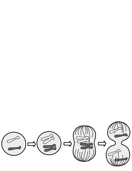
Figure 1. Cell division in eukaryotes.

It can also happen that a cell dies without division. Due to random events that occur both in and outside of a cell, its death without division as well as its lifetime span are random. In multicellular organisms, their tissues are built up with cells that constitute quite rigid structure and usually coordinate their evolution with each other, see Fig. 2.

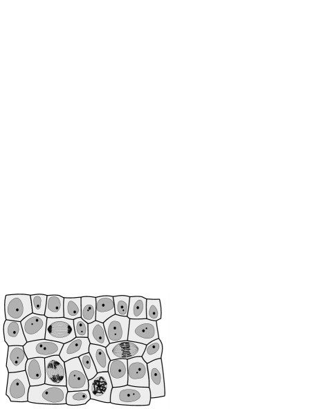
Figure 2. Cell structure of a healthy tissue.

Normally, developed organisms have more or less constant number of cells. If a cell dies, its neighbors receive the corresponding signal, and one of them undergoes division into two new cells. One of the progenies replaces the died cell, and thereby the overall balance is restored. There are two types of death: apoptosis and necrosis. The first one is a kind of programmed death of a cell that inevitably occurs to each of them. It is a part of the mechanism that controls the total number of cells in the organism. Necrosis is an accidental death that may occur, e.g., due to external factors. During the division of a cell mutations can occur. A mutation is the alteration of the nucleotide sequence of the cell genome. Mostly mutations are irrelevant and the organism functioning is unchanged. Such mutations are called neutral. Mutations in genes that regulate cell division, apoptosis, and DNA repair may cause uncontrolled cell proliferation, in the course of which the total number of cells gets bigger than usual (hyper- and dysplasia) that eventually leads to cancer. Such mutations propel the cells uncontrolled expansion and invasion [12]. ”Unlike normal cells, cancer cells ignore the usual density-dependent inhibition of growth … piling up until all nutrients are exhausted”, see Fig. 3, where the pictures going from the left present normal tissue, hyperplasia, mild dysplasia, severe dysplasia, and invasive cancer tissue, respectively. This illustrates the way of initiation of a cancer.

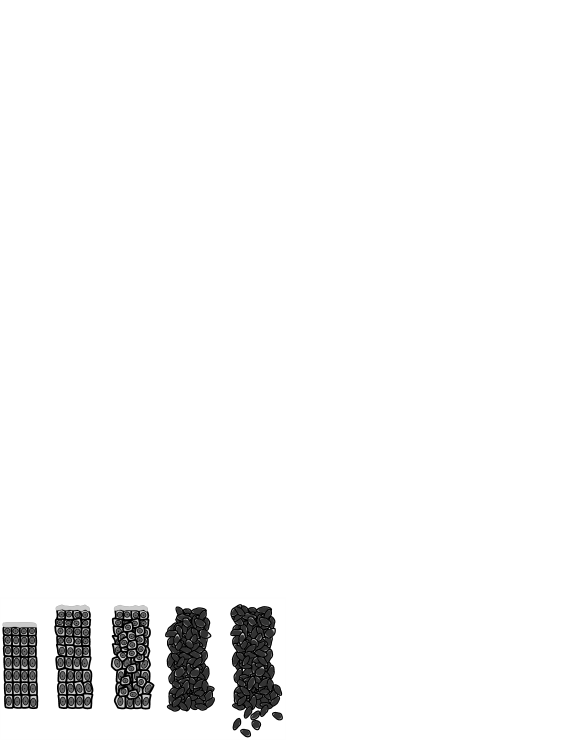
Figure 3. From normal tissue to invasive cancer.

.

2.2. Branching

Loosely speaking, branching is a process in which an entity – called a particle – produces at random a random number of offsprings. They repeat this action after some time. The state space of the process is the set of nonnegative integers $\mathbf{N}_{0}=\{0,1.\dots\}$. One of the simplest examples of branching is the Galton-Watson process, see Chapter 3 of [7]. In this case, every particle produces $k\in\mathbf{N}_{0}$ offsprings with probability $p_{k}\geq 0$ – independently of each other. The lifetime of all of the particles is the same. In view of this, one may distinguish generations in their population. Let $Z_{n}$ be the number of particles in $n$-th generation. It is a random variable with values in $\mathbf{N}_{0}$. The recurrence between the generations is obviously the following one

$$Z_{n+1}=\sum_{j=1}^{Z_{n}}X_{n,j},\qquad n\in\mathbf{N}_{0},$$ (2.1)

where $X_{n,j}$ is the number of offsprings of $j$-th member of generation $n$. By our assumption all these random variables $X_{n,j}$ are independent and identically distributed, and the event $X_{n,j}=k$ has probability $p_{k}\geq 0$, where the collection $(p_{k})_{k\in\mathbf{N}_{0}}$ is assumed given. Note that the sum in (2.1) has random number of summands, and also that $\sum_{k}p_{k}=1$. Usually, one assumes that the mean number of offsprings is finite, i.e.,

$$a:=\langle X_{n,j}\rangle=\sum_{k=0}^{\infty}kp_{k}<\infty.$$ (2.2)

If the number of particles in $n$-th generation is known, then the conditional expected number of them in the next generation is

$$\langle Z_{n+1}\rangle|_{Z_{n}}=\sum_{j=1}^{Z_{n}}\langle X_{n,j}\rangle=aZ_{n}.$$

By iterating the latter, cf. (2.1), we then get the unconditional expectation

$$\langle Z_{n}\rangle=a^{n}N_{0},$$ (2.3)

where $N_{0}$ is the (non-random) number of particles in the initial generation. The value $a=1$ is critical. For $a<1$, the branching process described by the recurrence (2.1) is sub-critical, cf. [7, page 11], in which the average number of offsprings of a particle is less than one. By (2.3) we then get $\langle Z_{n}\rangle\to 0$ as $n\to+\infty$, that means extinction of the population. For $a>1$, the branching process is super-critical, which means that $Z_{n}\to+\infty$ with high probability. Note that, for $p_{0}>0$, there may exist nonzero probability that the process dies out even in this supercritical case.

2.3. Dynamics: deterministic and stochastic

Now we turn to basic aspects of stochastic evolution. First, we introduce general notions, and then pay attention to an important feature of the stochastic counterpart.

2.3.1. Dynamical systems

Let $S$ be a nonempty set elements of which are considered as states of a given system. Such sets are called phase spaces. Usually, $S$ is endowed with mathematical attributes, such as topology and the corresponding Borel $\sigma$-field of its subsets. This allows one to define on $S$ probability measures, the set of which is denoted as $\mathcal{P}(S)$. As an example, one can keep in mind a harmonic oscillator for which $S=\mathbf{R}^{2}$ – the set of pairs $s=(q,p)$, where real $q$ and $p$ are position and momentum of the oscillator, respectively. Another example can be $S=\mathbf{N}_{0}$, see the Galton-Watson model above. In such a case, in state $n\in\mathbf{N}_{0}$ the system consists of $n$ elements, say particles. Then a (continuous time) dynamical system is a map $(t,s)\mapsto s_{t}\in S$ such that $s_{0}=s$. Here $t$ is time and $s$ is the initial state – origin of the trajectory $(s_{t})_{t\geq 0}$. Often, such trajectories are obtained by solving (if possible) differential equations, called evolution equations. For the mentioned harmonic oscillator, these equations are

$$\dot{q}_{t}=p_{t}/m,\qquad\dot{p}_{t}=-kq_{t},$$ (2.4)

where dot means time derivative and $m$ and $k$ are oscillator’s mass and rigidity, respectively. Then the trajectory $(q_{t},p_{t})$ is obtained – as the corresponding trigonometric functions – by solving (2.4). There exists another way of describing such evolutions, especially useful if the direct solving like in the case of (2.4) is impossible. It is based on the use of observables, which are suitable functions $F:S\to\mathbf{R}$. In this setting, $F(s)$ is the value of observable $F$ in state $s$ and the evolution $F\to F_{t}$ is defined by the identity $F_{t}(s)=F(s_{t})$, i.e., it is backward in this sense. In the Hamiltonian case of (2.4), the backward evolution equation is

$$\dot{F}_{t}(q,p)=\frac{\partial F_{t}(q,p)}{\partial q}\frac{\partial H(q,p)}{\partial p}-\frac{\partial F_{t}(q,p)}{\partial p}\frac{\partial H(q,p)}{\partial q},$$ (2.5)

where $H=p^{2}/2m+kq^{2}/2$ is oscillator’s Hamiltonian. Equations like (2.4), (2.5) describe deterministic evolution. To take into account random events that may occur in the system, one ought to employ probability measures $\mu\in\mathcal{P}(S)$ as system states. Then the value of observable $F$ in state $\mu$ is given by the following integral

$$\mu(F)=\int_{S}F(s)\mu(ds),$$ (2.6)

with the possibility to include point states $s\in S$ into this picture by associating them with Dirac measures $\delta_{s}$. The evolution now is a map $(t,\mu)\mapsto\mu_{t}\in\mathcal{P}(S)$, where $\mu$ is the initial state. This evolution is deterministic if $\mu=\delta_{s}$ implies $\mu_{t}=\delta_{s_{t}}$ for some $s_{t}\in S$, holding for all $t>0$. In other words, this evolution preserves the set of Dirac measures. Otherwise, it is called stochastic.

2.3.2. Honest stochastic evolutions

Now we turn to the Galton-Watson example in which $S=\mathbf{N}_{0}$. Let $\mu$ be a state on this $S$. Then it is defined by its values on singletons $\{n\}$, denoted by $\mu(n)$. That is, $\mu(n)$ is the probability of the event “the system consists of $n$ particles”. and the number $\mu(A)$ is the probability that the state of the system lies in $A\subset S$. Obviously, $\mu(S)=1$ as $\mu$ is a probability measure. In the course of evolution $(t,\mu)\mapsto\mu_{t}$, it may happen that, for some $t>0$, $\mu_{t}(S)<1$, i.e., $\mu_{t}$ fails to satisfy the mentioned condition, even if the initial state $\mu$ does. In the mentioned example, this corresponds to

$$\mu_{t}(\mathbf{N}_{0})=\sum_{n\geq 0}\mu_{t}(n)<1.$$

That is, the probability of having at time $t$ any finite number of particles is less than one, and then $1-\mu_{t}(\mathbf{N}_{0})>0$ is the probability that the system is infinite at this time, which means its explosion. Thus, the system explodes with positive probability if this occurs. This is similar to the extinction with positive probability of a supercritical branching process mentioned above. The evolution $(t,\mu)\mapsto\mu_{t}$ such that $\mu_{t}(S)=1$ for all $t>0$ is called honest. In this case, no explosion occurs. Obviously, honesty of the evolution of population of tumor cells is an extremely important aspect of the theory. Further details on honest stochastic evolutions can be found [9, 10, 11].

3. The Model

As mentioned above, we are aiming at showing the power of modeling with the help of an individual-based model[8] that describes the proliferation of tumor cells. Here “individual-based” means that the evolution of each single cell is taken into account explicitly – in contrast to phenomenological models [2, 12, 13, 14] where a population of cells is considered as a medium characterized by, e.g., density. Before introducing the model, we formulate basic principles and provide heuristic arguments intimating possible outcomes of its study.

3.1. Basic arguments

A standard approach to curing cancer can schematically be presented as follows. The main part of the bulk tumor is removed by surgery, and the remaining tumor cells are then treated by chemo- and/or radio-therapy aiming at their extinction. As the therapy can also affect healthy tissue, an essential aspect of the method is minimizing the therapeutic pressure needed to achieve the aim. The considered model is intended to describe the evolution of the remaining population of tumor cells and thus to estimate their minimal mortality that guarantees the mentioned extinction. Its construction is based on the following principles.

• The population of cells is finite. Each of its members is characterized by its lifetime (length of its cycle). The lifetimes of the cells are independent and identically distributed random variables, the common distribution of which is known. At the end of its cycle, a cell divides into two progenies.

• Each cell can die before producing progenies. The death is caused solely by the therapeutic pressure and is independent of the total number of cells. That is, we do not take into account natural death (untreated tumor cells are ‘immortal’, cf. [7, page 28]) and competition-caused mortality – essential in the bulk tumor and minor after its removal.

According to (a), the lifetime $\tau$ of a given cell is random. Assume for a while that it is deterministic and the same for all cells, that is the cells behave as in the Galton-Watson model mentioned above, with strictly positive $p_{0}$ and $p_{2}$ and $p_{k}=0$ otherwise. Clearly, $p_{0}$ is the probability of the premature death (due to therapy), and $p_{2}=1-p_{0}$. To calculate $p_{0}$ we need to choose the way of realizing the therapeutic pressure. In its simplest and most realistic version, the probability of staying alive for a given cell diminishes with constant speed $-m$, where the mortality parameter $m>0$ is assumed to be the same for all cells. Its value depends only on the therapy and (in principle) may be estimated, e.g., in vitro. According to this, the probability in question is $e^{-mt}$. At the end of the life period we have $t=\tau$; hence, $p_{2}=e^{-m\tau}$ and $p_{0}=1-e^{-m\tau}$. Then the branching parameter $a$ is, cf. (2.2),

$$a(\tau)=0\cdot(1-e^{-m\tau})+2\cdot e^{-m\tau}=2e^{-m\tau}.$$ (3.1)

Now we take into account that $\tau$ is random. Assume that its probability distribution has density (with respect to Lebesgue’s measure) given by an appropriate function $g$. Then the averaged branching parameter is

$$\langle a\rangle=\int_{0}^{+\infty}a(\tau)g(\tau)d\tau=2\int_{0}^{+\infty}e^{-m\tau}g(\tau)d\tau=2\widehat{g}(m),$$ (3.2)

where $\widehat{g}$ is the Laplace transform of $g$, see, e.g., [15]. Now the extinction condition takes the form

$$\widehat{g}(m)<\frac{1}{2}.$$ (3.3)

Since $g$ is positive and integrable, $\widehat{g}(m)$ decays to zero in a monotone way as $m\to+\infty$. At the same time, $\widehat{g}(0)=1$ due to normalization. Thus, (3.3) can be satisfied at the cost of large enough mortality. Let $m_{*}$ be the (unique) solution of the equation

$$\widehat{g}(m)=\frac{1}{2}.$$ (3.4)

Then (3.3) is satisfied for all $m>m_{*}$. For various kinds of tumor, the distribution of $\tau$ is well-studied, see [4, 16] and also [17, 18, 19]. Usually, one takes

$$g(\tau)=\frac{\tau^{k-1}e^{-\tau/\theta}}{\theta^{k}\varGamma(k)},\qquad k,\theta\in(0,+\infty),$$ (3.5)

that is the density of the $\varGamma$-distribution, cf. [17, 19] and see Fig. 4. Here $\varGamma(k)$ is Euler’s $\varGamma$-function.

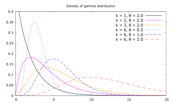
Figure 4. Density $g$ of the $\varGamma$-distributions, see (3.5), for various values of $k$ and $\theta$.

In this case,

$$\widehat{g}(m) = \frac{1}{\theta^{k}\varGamma(k)}\int_{0}^{+\infty}\tau^{k-1}\exp\left(-m\tau-\frac{\tau}{\theta}\right)d\tau$$

$$= \frac{1}{(1+m\theta)^{k}\varGamma(k)}\int_{0}^{+\infty}x^{k-1}e^{-x}dx$$

$$= (1+m\theta)^{-k},$$

and then the condition in (3.3) is satisfied for $m>m_{*}$ where

$$m_{*}=\frac{1}{\theta}\left(2^{1/k}-1\right).$$ (3.7)

3.2. Towards introducing the model

In accordance with the principles formulated above, the model in words can be described as follows. Consider a finite subset of $\mathbf{R}_{+}:=[0,+\infty)$ – a cloud of point particles. Then the coordinate $x\in\mathbf{R}_{+}$ of a particle in this cloud is considered as its time to division. The basic act of the evolution is aging – drifting towards the point $x=0$ with unit speed. That is, we assume time to division diminishes with speed one. By reaching the origin the particle divides into two new particles – progenies – that appear at random positions on the half-line $\mathbf{R}_{+}$. Thereafter, the progenies start drifting towards $x=0$. During its lifetime, i.e., before division, each particle can be removed at random with constant (mortality) rate $m>0$. Since the point states of the system are mentioned clouds, to describe them we will employ notions and methods of the theory of point processes [20].

Let $\Gamma$ denote the set of all finite subset of $\mathbf{R}_{+}$. Its elements are finite clouds mentioned above. This is the phase space of the population of tumor cells for our model. It is equipped with the weak topology which is metrizable in such a way that the corresponding metric space is separable and complete. Note that a complete characterization of the weak topology is: a sequence, $\{\gamma_{n}\}_{n\in\mathbf{N}}\subset\Gamma$, is convergent in this topology to some $\gamma\in\Gamma$ if

$$\sum_{x\in\gamma_{n}}g(x)\to\sum_{x\in\gamma}g(x),$$

that holds for all bounded continuous functions $g:\mathbf{R}_{+}\to\mathbf{R}$. Let $\mathcal{B}(\Gamma)$ be the corresponding Borel $\sigma$-field. A function, $f:\Gamma\to\mathbf{R}$, is then measurable if there exists a collection of symmetric Borel functions $f^{(n)}:\mathbf{R}^{n}_{+}\to\mathbf{R}$, $n\in\mathbf{N}$, such that

$$f(\{x_{1},\dots,x_{n}\})=f^{(n)}(x_{1},\dots,x_{n}),\qquad n\in\mathbf{N}.$$ (3.8)

We also set $f^{(0)}=f(\varnothing)$. In expressions like $\gamma\cup x$, $x\in\mathbf{R}_{+}$ we consider $x$ as a single-element configuration $\{x\}$. The Lebesgue-Poisson measure $\lambda$ on $(\Gamma,\mathcal{B}(\Gamma))$ is defined by the integrals

$$\int_{\Gamma}f(\gamma)\lambda(d\gamma)=f^{(0)}+\sum_{n=1}^{\infty}\frac{1}{n!}\int_{\mathbf{R}_{+}^{n}}f^{(n)}(x_{1},\dots,x_{n})dx_{1}\cdots dx_{n},$$ (3.9)

holding for all bounded measurable $f:\Gamma\to\mathbf{R}$. Such integrals have the following evident property

$$\int_{\Gamma}\left(\sum_{\xi\subset\gamma}f(\gamma,\xi)\right)\lambda(d\gamma)=\int_{\Gamma}\int_{\Gamma}f(\gamma\cup\xi,\xi)\lambda(d\gamma)\lambda(d\xi).$$ (3.10)

Let $\mathcal{E}$ denote the real Banach space $L^{1}(\Gamma,d\lambda)$. Its positive elements constitute the cone $\mathcal{E}^{+}$. The norm of $\mathcal{E}$ then is

$$\|f\|=\int_{\Gamma}|f(\gamma)|\lambda(d\gamma).$$ (3.11)

Hence, probability densities are elements of $\mathcal{E}^{+}$ of unit norm.

For a given $n\in\mathbf{N}$, by $\mathcal{W}^{1,1}_{n}$ we denote the standard Sobolev space[21] on $(0,+\infty)^{n}$, whereas $\mathcal{W}^{1,1}_{n,s}$ will stand for its subset consisting of all symmetric $u$, i.e., such that $u(x_{1},\dots,x_{n})=u(x_{\sigma(1)},\dots x_{\sigma(n)})$ holding for all permutations $\sigma\in\varSigma_{n}$.

Remark 3.1.

By Theorem 1, page 4 of Ref. [21] we know that each element of $\mathcal{W}^{1,1}_{n,s}$ – as an equivalence class – contains a unique (symmetric) $u:\mathbf{R}^{n}_{+}\to\mathbf{R}$ such that

• for Lebesgue-almost all $(x_{1},\dots,x_{n-1})$, the map $\mathbf{R}_{+}\ni y\mapsto u(y,x_{1}\dots,x_{n-1})$ is continuous and its restriction to $(0,+\infty)$ is absolutely continuous;

• the following holds

  $$\int_{\mathbf{R}_{+}^{n}}\left|\frac{\partial}{\partial x_{1}}u(x_{1},\dots,x_{n})\right|dx_{1}\cdots dx_{n}<\infty.$$

In the sequel, we will mean this function $u$ when speaking of a given element of $\mathcal{W}^{1,1}_{n,s}$.

Let $f$ and $f^{(n)}$ be as in (3.8), (3.9). Let also $\mathcal{W}$ be then the set of all $f$ for which $f^{(n)}\in\mathcal{W}^{1,1}_{n,s}$. Define

$$(Df)^{(n)}(x_{1},\dots,x_{n}) = \sum_{j=1}^{n}\frac{\partial}{\partial x_{j}}f^{(n)}(x_{1},\dots,x_{n})$$

$$= \frac{d}{dt}f^{(n)}(x_{1}+t,\dots,x_{n}+t)|_{t=0}.$$

This allows us to define also

$$(Df)(\gamma)=\frac{d}{dt}f(\gamma_{t})|_{t=0},$$ (3.13)

$$f(\gamma_{t})=f(\gamma)+\int_{0}^{t}(Df)(\gamma_{\tau})d\tau.$$

Note that

$$\|Df\| := \sum_{n=1}^{\infty}\frac{1}{n!}\int_{\mathbf{R}_{+}^{n}}\sum_{j=1}^{n}\left|\frac{\partial}{\partial x_{j}}f^{(n)}(x_{1},\dots,x_{n})\right|dx_{1}\cdots dx_{n}$$

$$= \sum_{n=0}^{\infty}\frac{1}{n!}\int_{\mathbf{R}_{+}^{n+1}}\left|\frac{\partial}{\partial x}f^{(n+1)}(x,x_{1},\dots,x_{n})\right|dxdx_{1}\cdots dx_{n}<\infty,$$

whenever $f\in\mathcal{W}$. The key issue in (3.2) is the convergence of the series. In (3.13), we use shifts of $\gamma\in\Gamma$. For $t\in\mathbf{R}$, we set $\gamma_{t}=\{x+t:x\in\gamma\}$. For $t>0$, this is well-defined for all $\gamma$, whereas for $t<0$ one should apply such shifts only to proper $\gamma$, i.e., such that $x+t\geq 0$ for all $x\in\gamma$.

For $f\in\mathcal{W}$, we define

$$\|f\|_{\mathcal{W}}=\|f\|+\|Df\|,$$ (3.15)

which is finite in view of (3.2), see also (3.11). It is possible to prove the following statement, see Proposition 2.2 in [8].

Proposition 3.2.

The set $\mathcal{W}$ equipped with the norm defined in (3.15) is a Banach space. Thus, the linear operator $(D,\mathcal{W})$ defined on $\mathcal{E}$ in (3.2) and (3.2) is closed.

3.3. Defining the model

In our approach, the stochastic evolution of the considered population of tumor cells is Markovian. According to the basic principles formulated above it is described by the following backward Kolmogorov equation

$$\frac{d}{dt}F_{t}=L^{*}F_{t},\qquad F_{t}|_{t=0}=F_{0},$$ (3.16)

with

$$(L^{*}F)(\gamma) = -(DF)(\gamma)+\sum_{x\in\gamma}m\left[F(\gamma\setminus x)-F(\gamma)\right]$$

$$+ \sum_{x\in\gamma}\delta(x)\int_{\mathbf{R}_{+}^{2}}G(y,z)\left[F(\gamma\setminus x\cup\{y,z\})-F(\gamma)\right]dydz,$$

where $F_{t}:\Gamma\to\mathbf{R}$ is an observable. Here (3.16) (with $L^{*}$ given in (3.3)) corresponds to the backward evolution equation (2.5) mentioned above. The first term in (3.3) describes aging – the drift of the trait “time to division” towards the origin, and thus is of gradient form. The second term describes the mortality caused by the therapy with mortality rate $m\geq 0$ – the same as in (3.1), (3.2). The last term describes the division of the cells. Therein, $\delta(x)$ is the Dirac $\delta$-function and $G(x,y)$ is the probability density of the distribution of lifetimes of the two progenies. It thus satisfies the normalization condition

$$\int_{\mathbf{R}_{+}^{2}}G(x,y)dxdy=1.$$

Obviously, $G(x,y)$ is symmetric and such that

$$g(x)=\int_{\mathbf{R}_{+}}G(x,y)dy,$$

is the same as in (3.1) and (3.2). Since the right-hand side of (3.3) contains a distribution, possible solutions of (3.16) ought to be distributions as well, which may cause essential technical problems. To avoid them one can pass to a forward Kolmogorov equation, called also Fokker-Planck equation. To this end one employs the identity

$$\int_{\Gamma}F(\gamma)(Lf)(\gamma)\lambda(d\gamma)=\int_{\Gamma}(L^{*}F)(\gamma)f(\gamma)\lambda(d\gamma),$$ (3.18)

and the rule (3.10). After some calculations it yields the Fokker-Planck equation

$$\frac{d}{dt}f_{t}=Lf_{t},\qquad f_{t}|_{t=0}=f_{0}.$$ (3.19)

Here $f_{0}$ is the probability density of the initial state $\mu_{0}$. That is,

$$\mu_{0}(d\gamma)=f_{0}(\gamma)\lambda(d\gamma),$$

where $\lambda$ is the Lebesgue-Poisson measure defined in (3.9). Likewise, $f_{t}$ is the probability density of the state $\mu_{t}$ at time $t>0$. In accordance with (3.18), the operator in (3.19) has the following form

$$(Lf)(\gamma)=(Df)(\gamma)+m\int_{\mathbf{R}_{+}}f(\gamma\cup x)dx$$ (3.20)

$$-m|\gamma|f(\gamma)+2\sum_{\{x,y\}\subset\gamma}G(x,y)f(\gamma\setminus\{x,y\}\cup 0),$$

where $|\gamma|$ is the number of points in $\gamma\in\Gamma$. Our aim is to solve (3.19) and thereby to describe the evolution of the population. Regarding $G$ we will assume the following. For $\beta>0$, we define

$$\psi_{\beta}(x)=\frac{1}{(1+x)^{\beta}},\qquad x\geq 0.$$

Then the cell cycle distribution is such that the probability density $G$ satisfies the condition: there exist $b>0$ and $\beta\geq 3$ such that, for all $x,y\geq 0$, the following holds

$$G(x,y)\leq b\left[\psi_{\beta+1}(x)\psi_{\beta}(y)+\psi_{\beta}(x)\psi_{\beta+1}(y)\right].$$ (3.21)

The equation in (3.19) should be considered in the Banach space $\mathcal{E}$ introduced above. The usual way of studying such evolution equations is to use strongly continuous semigroups of bounded linear operators in such spaces[22, 23, 24]. To this end, one has to define $L$ as an unbounded linear operator in $\mathcal{E}$, which includes also defining its domain. We begin this by writing

$$L=A+B=A+B_{1}+B_{2},$$ (3.22)

$$(Af)(\gamma)=(Df)(\gamma)-m|\gamma|f(\gamma),$$

$$(B_{1}f)(\gamma)=2\sum_{\{x,y\}\subset\gamma}G(x,y)f(\gamma\setminus\{x,y\}\cup 0),$$

$$(B_{2}f)(\gamma)=m\int_{\mathbf{R}_{+}}f(\gamma\cup x)dx.$$

Note that both $B_{i}$ are positive. Without treatment tumor cells would certainly proliferate ad infinitum. In view of this, from now on we assume that the mortality rate $m$ is strictly positive, and then set

$$h_{m}(\gamma)=1+m|\gamma|.$$ (3.23)

Recall that $|\gamma|$ denotes the number of points in $\gamma$. Along with the space $\mathcal{E}$ we also use the following weighted Banach space $\mathcal{E}_{m}=L^{1}(\Gamma,h_{m}d\lambda)$ equipped with the norm

$$\|f\|_{m}=\int_{\Gamma}|f(\gamma)|h_{m}(\gamma)\lambda(d\gamma).$$ (3.24)

By (3.24) and then by (3.22), (3.23) one gets

$$\|B_{2}f\|\leq\|f\|_{m}.$$ (3.25)

For positive $f\in\mathcal{W}$, by means of (3.10) one can produce the following calculations

$$\|B_{1}f\| = 2\int_{\Gamma}\left(\sum_{\{x,y\}\subset\gamma}G(x,y)f(\gamma\setminus\{x,y\}\cup 0)\right)\lambda(d\gamma)$$

$$= \int_{\Gamma}\left(\sum_{x\in\gamma}\sum_{y\in\gamma\setminus x}G(x,y)f(\gamma\setminus\{x,y\}\cup 0)\right)\lambda(d\gamma)$$

$$= \int_{\Gamma}\left(\int_{\mathbf{R}{+}}\sum_{y\in\gamma}G(x,y)f(\gamma\setminus y\cup 0)dx\right)\lambda(d\gamma)$$

$$= \int_{\Gamma}\left(\int_{\mathbf{R}_{+}^{2}}G(x,y)dxdy\right)f(\gamma\cup 0)\lambda(d\gamma)=\|Df\|.$$

That is, $B_{1}$ and $D$ can be defined on $\mathcal{W}\subset\mathcal{E}$. Keeping this and (3.25) in mind we set

$$\mathcal{D}(A)=\mathcal{W}\cap\mathcal{E}_{m},\qquad\mathcal{D}^{+}(A)=\mathcal{D}(A)\cap\mathcal{E}^{+}.$$ (3.27)

By (3.25) and (3.3) we then conclude that

$$B:\mathcal{D}(A)\to\mathcal{E}.$$

3.4. The result

Along with $h_{m}$ defined in (3.23) we use

$$w_{\sigma,\alpha}(\gamma)=1+\sigma|\gamma|+\sum_{x\in\gamma}e^{-\alpha x},\qquad\gamma\in\Gamma,$$ (3.28)

with some positive $\sigma$ and $\alpha$. Define, cf. (3.24),

$$\|f\|_{\alpha,\sigma}=\int_{\Gamma}|f(\gamma)|w_{\sigma,\alpha}(\gamma)\lambda(d\gamma).$$ (3.29)

Recall that we assume (3.21) holding with $\beta\geq 3$ and $b>0$. Keeping this in mind we then set

$$m_{0}=\left\{\begin{array}[]{ll}\frac{(\beta-1)(b-\beta)}{2\beta-5},&{\rm if}\ \ b>\beta;\\[11.38092pt] 0&{\rm otherwise}.\end{array}\right.$$ (3.30)

Along with this parameter we also introduce

$$m_{1}=\max\{m_{0};m_{*}\},$$ (3.31)

where $m_{*}$ is defined in (3.4). In the case of $\varGamma$-distributions, it is given in (3.1) and (3.7).

Let us now make precise in which sense we are going to solve the Cauchy problem in (3.19). By its classical solution, cf. Chapter 4 in [23], with $f_{0}\in\mathcal{D}(L)$ we understand a function $t\mapsto f_{t}\in\overline{\mathcal{D}(A)}\subset\mathcal{E}$ which is: (a) continuously differentiable at all $t\geq 0$; (b) such that both equalities in (3.19) are satisfied. Here $\overline{\mathcal{D}(A)}$ denotes the domain of the closure of $L=A+B$, which is the closure of $\mathcal{D}(A)$ in the graph norm. Then the main statement describing the evolution of the considered population of tumor cells reads as follows, see Theorem 2.7 in [8].

Theorem 3.3.

Assume that (3.21) holds with some $\beta\geq 3$ and $b>0$. Then, for each $m>m_{0}$ (defined in (3.30)) and $f_{0}\in\mathcal{D}^{+}_{1}(A):=\{f\in\mathcal{D}^{+}(A):\|f\|=1\}$, see (3.27), the Fokker-Planck equation (3.19) has a unique classical positive solution $f_{t}$ such that $\|f_{t}\|=1$. Furthermore, for $m>m_{1}$ defined in (3.31), there exists $\sigma>0$ for which $\|f_{t}\|_{\alpha,\sigma}\leq\|f_{0}\|_{\alpha,\sigma}$ holding for all $t>0$.

The meaning of this mathematical statement will be discussed in the concluding part of the chapter.

3.5. Sketch of the proof

The proof of Theorem 3.3 is based on a version of the perturbation theory for generators of stochastic semigroups [24]. Its details are similar to those of the proof of the corresponding statement in [8]. Here we just outline its main steps. One begins by proving that, for each $\varepsilon>0$, the operator

$$L_{\varepsilon}:=A+\varepsilon B,$$

see (3.22), with domain $\mathcal{D}(L_{\varepsilon})=\mathcal{D}(L)$ defined in (3.27), is the generator of a substochastic semigroup $S_{\varepsilon}=\{S_{\varepsilon}(t)\}_{t\geq 0}$. Here ‘substochastic’ means that it is positive, i.e., $S(t):\mathcal{E}^{+}\to\mathcal{E}^{+}$, and such that $\|S_{\varepsilon}(t)f\|\leq\|f\|$, holding for all $t>0$. According to [24], $L$ as given in (3.22) is the generator of a positive semigroup $S=\{S(t)\}_{t\geq 0}$ that is obtained from $S_{\varepsilon}$ in the limit $\varepsilon\to 0$. Then the unique solution of (3.19) is obtained in the form

$$f_{t}=S(t)f_{0}.$$ (3.32)

However, the limiting semigroup $S$ may be only substochastic – not stochastic, and hence the evolution $f_{0}\to f_{t}=S(t)f_{0}$ may be dishonest. The proof of its honesty – based on the condition $m>m_{0}$, see (3.30) – is then conducted by means of a result of [10]. The proof of the second part is conducted with the help of methods of [24] by which we show that the semigroup $S$ preserves the norm of $f$ defined in (3.29) whenever $m>m_{1}$. That is, under the latter condition one has

$$\|S(t)f_{0}\|_{\alpha,\sigma}\leq\|f_{0}\|_{\alpha,\sigma},$$

holding for all $t>0$ and some $\alpha$ and $\sigma$. By (3.32) this yields the property in question.

3.6. Concluding remarks

First of all we make some comments on the results of Theorem 3.3. By this statement the expected number of cells at time $t$ is

$$N(t)=\int_{\Gamma}|\gamma|f_{t}(\gamma)\lambda(d\gamma),$$

where $|\gamma|$ stands for the number of points in $\gamma$. By (3.28) and (3.29) we then conclude that

$$N(t)\leq\sigma^{-1}\|f_{t}\|_{\alpha,\sigma}\leq\sigma^{-1}\|f_{0}\|_{\alpha,\sigma},$$

holding for all $t>0$ and $m>m_{1}$. Then a therapeutic outcome of Theorem 3.3 is that the number of tumor cells will not increase in time whenever the latter condition is satisfied. This may determine the minimal level of the therapeutic pressure needed to achieve this goal. Second, we note that the fulfilment of the condition $m>m_{0}$ guarantees that the evolution $f_{0}\to f_{t}$ is honest since $f_{t}$ is positive and $\|f_{t}\|=1$. If $m_{0}=0$, which is the case if $b\leq\sigma$, then the condition $m>m_{1}$ coincides with that in (3.3). Hence, in this case the heuristic arguments leading to (3.3) give the same answer as the microscopic modeling resulting in Theorem 3.3. One cannot exclude, however, that the evolution $f_{0}\to f_{t}$ fails to be honest for $m\in(m_{*},m_{0}]$ if $m_{0}>m_{*}$. In this case, the individual-based modeling yields a more precise result that is unaccessible by heuristic theories. Note also that $b$ takes into account possible dependence between the siblings cycle lengths, totally ignored in the heuristic deduction of (3.3).

Finally, the model defined by $L$ introduced in (3.20) can be modified to take into account the following aspects: (a) variability of the distribution of the lifetimes of offsprings; (b) variability of the death rate $m$. Aspect (a) means that the density function $G$ of a cell may be different from that of her daughters. This can be realized by adding an additional trait $y\in Y$ with a suitable set $Y$. The change of this trait might then be related to mutations. Aspect (b) means dependence of $m$ on $y$ that takes into account, e.g., drug resistance acquired in the course of mutations. In the mathematics, introducing $y$ will correspond to passing from single $x$ to compound traits $(x,y)$, and thus to dealing with marked configurations, see [25] and the papers quoted therein. We plan to study this model in a forthcoming work.

References

- [1] Yu. Kozitsky, Mathematical theory of the Ising model and its generalizations: an introduction, in Order, disorder and criticality, Advanced problems of Phase Transitions Theory, Vol. 1, by Yu. Holovatch (ed.), World Scientific (Singapore, 2004), pp. 1–66.
- [2] S. Benzekry , C. Lamont, A. Beheshti, A. Tracz, J. M. L. Ebos, L. Hlatky and Ph. Hahnfeldt, Classical mathematical models for description and prediction of experimental tumor growth, PLOS, Comput. Biology 10(8), e1003800 - 19 pp (2014).
- [3] M. J. Kim, R. J. Gillies and K. A. Rejniak, Current advances in mathematical modeling of anti-cancer drug penetration into tumor tissues, Front. Oncol. 3, 278 - 10 pp. (2013).
- [4] A. Swierniak, M. Kimmel and J. Smieja, Mathematical modeling as a tool for planning anticancer therapy, European Journal of Pharmacology 625, 108–121 (2009).
- [5] D. Drasdo and S. Höhme, A single-cell-based model of tumor growth in vitro: monolayers and spheroids, Phys. Biol. 2(3) , 133–147 (2005).
- [6] P. Chen, B. Li and X. Feng, A cell-based model for analyzing growth and invasion of tumor spheroids, Sci. China Technol. Sci. 62(8), 1341–1348 (2019).
- [7] M. Kimmel and D. E. Axelrod, Branching Processes in Biology. Springer, New York, (2002).
- [8] Yu. Kozitsky, Stochastic branching at the edge: Individual-based modeling of tumor cell proliferation, arxiv:1910.12962, (2019).
- [9] L. Arlotti, B. Lods, M. Mokhtar-Kharroubi, On perturbed substochastic semigroups in abstract state spaces, Z. Anal. Anwend. 30, 457–495, (2011).
- [10] M. Mokhtar-Kharroubi, New generation theorems in transport theory, Afr. Math. 22, 153–176, (2011).
- [11] G. E. H. Reuter, Denumerable Markov processes and the associated contraction semigroups on , Acta Math. 97, 1–46, (1957).
- [12] J. Evan and K. Vousden, Proliferation, cell cycle and apoptosis in cancer, Nature 411, 342–348 (2001).
- [13] J. L. Lebowitz and S. I. Rubinow, A theory for the age and generation time distribution of a microbial population, J. Math. Biology. 1(1), 17–36 (1974).
- [14] M. Rotenberg, Transport theory for growing cell populations, J. Theor. Biol. 103, 181–199, (1983).
- [15] G. Doetsch, Introduction to the Theory and Application of the Laplace Transformation. Springer, Berlin Heidelberg (1974).
- [16] M. Dolbniak, M. Kimmel and S. Smieja, Modeling epigenetic regulation of PRC1 protein accumulation in the cell cyclem, Biology Direct 10 62, 15 pp, (2015).
- [17] P. Gabriel, S. P. Garbett, V. Quaranta, D. R. Tyson and G. F. Webb, The contribution of age structure to cell population responses to targeted therapeutics, J. Theor. Biol. 311, 19–27, (2012).
- [18] D. R. Tyson, S. P. Garbett, P. L. Frick and V. Quaranta, Fractional proliferation: a method to deconvolve cell population dynamics from single-cell data, Nature Methods 9, 923–928, (2012).
- [19] Ch. A. Yates, M. J. Ford and R. L. Mort, Multi-stage representation of cell proliferation as a Markov process, Bull. Math. Biol. 79, 2905–2928, (2017).
- [20] D. J. Daley and D. Vere-Jones, An Introduction to the Theory of Point Processes. Vol. I. Elementary Theory and Methods. Second edition. Probability and its Applications (New York). Springer-Verlag, New York, (2003).
- [21] V. Maz’ya, Sobolev Spaces with Applications to Elliptic Partial Differential Equations. Second, revised and augmented edition. Grundlehren der Mathematischen Wissenschaften, 342. Springer, Heidelberg, (2011).
- [22] J. Banasiak and L. Arlotti, Perturbations of Positive Semigroups with Applications. Springer Monographs in Mathematics. Springer-Verlag London, Ltd., London, (2006).
- [23] A. Pazy, Semigroups of Linear Operators and Applications to Partial Differential Equations. Second edition. Applied Mathematical Sciences, 44. Springer-Verlag, New York Inc, (1983).
- [24] H. R. Thieme and J. Voigt, Stochastic semigroups: their construction by perturbation and approximation, in Positivity IV – Theory and Applications, by M. R. Weber and J. Voigt (eds.), Tech. Univ. Dresden (Dresden, 2006), pp. 135–146.
- [25] D. Jasińska and Yu. Kozitsky, Dynamics of an infinite age-structured particle system, arxiv:2001.06706, (2020).