Abstract

Predicting the number of coauthors for researchers contributes to understanding the development of team science. However, it is an elusive task due to diversity in the collaboration patterns of researchers. This study provides a learning model for the dynamics of this variable; the parameters are learned from empirical data that consist of the number of publications and the number of coauthors at given time intervals. The model is based on relationship between the annual number of new coauthors and time given an annual number of publications, the relationship between the annual number of publications and time given a historical number of publications, and Lotka’s law. The assumptions of the model are validated by applying it on the high-quality dblp dataset. The effectiveness of the model is tested on the dataset by satisfactory fittings on the evolutionary trend of the number of coauthors for researchers, the distribution of this variable, and the occurrence probability of collaboration events. Due to its regression nature, the model has the potential to be extended to assess the confidence level of the prediction results and thus has applicability to other empirical research.

Keywords: Coauthorship, Publication productivity, Data modelling.

Introduction

A growing trend of collaboration has emerged in current scientific research. This trend is reflected in increasingly active coauthorship among researchers as solitary authorship diminishes in prevalence[1]. Coauthorship has attracted much attention, with analyses of perspectives ranging from contribution[2, 3], population[4], discipline[5, 7, 6], country[9, 8], and multination[11, 12, 10, 13], to the connection with citations[14, 15]. The emerging field known as team science draws on diverse disciplinary perspectives to understand the processes and outcomes of scientific collaboration. Team work has been shown to have a large citation impact[16, 17], transdisciplinary outcomes[18], and high publication productivity[19]. Uzzi et al indicated that publications with three or more authors showed an increased frequency of “tail novelty” (which is a publication’s 10th-percentile $z$ score for its journal pairings) over the solo-author rate[20]. They used regression methods to analyze the relationship between the number of citations of a publication and the number of its authors, and found that publications produced by larger teams were associated with a higher citation impact. Wu et al found that the character of publications produced by large teams differs from that of small teams in terms of development versus disruption[21]. The number of coauthors is related to the team size. For example, more than 70% of researchers in the empirical dataset considered here belong to one team (see Appendix A). Therefore, the prediction has the potential to propose auxiliary measures for teams’ innovation, impact, and research character.

A previous study showed that the assembly mechanisms of a research team determine the structure of coauthorship networks[22, 23]. Much attention has been paid to these networks, and research has been concentrated on coauthor distribution[24, 25, 26], followed by structure[27, 28, 29], clustering[30], homophily[31, 32], and applications, e.g., name disambiguation[33]. Researchers have established a range of models, from preference attachment to cooperative game theory[34, 35, 36], to explore possible mechanisms for the evolution of the networks created by coauthorship. Most of these models generate a constant number of links for each new node, which is far from the reality. To simulate coauthorship networks at full scale, we need to know the extent to which researchers collaborate. Therefore, a method of predicting the number of coauthors is needed.

Researchers have explored possible factors that increase or decrease the number of new coauthors, such as the institutional prestige[37], self-organization[38], geography[39], discipline or interdiscipline[40], and academic reputation of researchers[41]. Knowledge of the correlated factors helps to predict the number of coauthors for a given researcher. However, factor analysis in social systems cannot exhaust all possible factors, as the considered factors would be correlated. For example, prestigious institutions that possess famous researchers can attract researchers to collaborate, which in part leads to multi-university collaborations[42]. Some have of the identified correlations between the considered factors and response variables may be caused by unconsidered factors or by the correlations between the considered factors, which are called spurious correlations. Therefore, analyzing factors individually is not recommended in statistical analysis. Accordingly, a multivariate statistical model to predict the number of coauthors is needed.

To choose suitable statistical models, we need to know the detailed features of the distributions of response variables and the mechanisms thereof. Coauthors appear in the process of producing publications; thus, there is a need to predict publication productivity. The number of publications of a researcher can be explained by an inhomogeneous Poisson process[43]. A model of piecewise Poisson regression has been proposed to predict the number of publications[44]. Its limitation regarding the prediction for highly productive researchers is solved by utilizing Lotka’s law[45]. Based on the high-quality dblp dataset, the effectiveness of these models has been tested by satisfactory fittings on the distribution and the evolutionary trend of the number of publications for researchers, as well as the occurrence probability of publication events.

This study proposes a learning model to utilize multiple factors to predict the number of coauthors for researchers. Three factors are used as a beginning, namely, time, the historical number of publications, and the historical number of coauthors. The piecewise Poisson regression on the training datasets extracted from the dblp dataset, given an annual number of publication, shows a significant correlation between the annual number of new coauthors of a researcher and time. However, the annual number of new coauthors does not follow a Poisson distribution. Therefore, using the piecewise Poisson regression and the predicted annual number of publications can provide only preliminary results for the number of coauthors. The results are modified by the formulae that address the cumulative advantage of attracting coauthors in terms of the historical number of coauthors. The hyperparameters of the formulae are determined by a genetic algorithm for a good fit to validation datasets. The effectiveness of the model is displayed by a good fit to the test datasets in terms of the evolutionary trend of the number of coauthors, the distribution of this variable, and the occurrence probability of collaboration events.

This paper is organized as follows. The model and its motivation are described in Sections 2, 3. The empirical data and experiments are described in Section 4. The results are discussed and conclusions drawn in Section 5.

Motivation

The relationship among time, the number of publications and coauthors

A positive correlation between the number of publications of a researcher and the number of his or her coauthors has been found in several empirical datasets[43], and is also found in the dataset analyzed here (see Appendix A). Correlation does not indicate causality, and arguments exist on whether scientific collaboration has a positive effect on publishing productivity. Lee et al found that the number of coauthors is not a significant predictor of the number of publications[46]. However, Ductor showed that after controlling for endogenous coauthorship formation, unobservable heterogeneity, and time, the effect of intellectual collaboration on the number of an individual’s publications becomes positive[47]. Therefore, our model does not include the correlation.

The analysis on the dblp dataset shows that given an annual number of publications, the annual number of a researcher’s new coauthors significantly correlates to time. Therefore, the annual number of new coauthors can be predicted when the future annual number of publications is known. A previous model can predict the latter variable[45], which makes it possible to predict the former variable. Note that the analysis on the dblp dataset shows that the annual number of new coauthors does not significantly correlate to time when considering all individuals or individuals with the same historical number of publications. Therefore, the annual number of publications is utilized in our model as a middle variable.

The distribution of the number of coauthors

In our study, the coauthor distribution of a group of researchers refers to the distribution of the number of a researcher’s coauthors. To choose a suitable regression model, we need to know the distribution features of the response variables and the mechanisms that generate these features. The number of coauthors of a researcher, as a response variable, is in part dependent on his or her number of publications. Previous studies on several empirical datasets have shown that the distribution of the number of a researcher’s publications is characterized by a trichotomy, comprising a generalized Poisson head, a power-law midsection, and an exponential cutoff[43]. The trichotomy can be derived from a range of “coin-flipping” behaviors, in which the probability of observing “heads” is dependent on events already observed [48].

The event of producing a publication can be regarded as an analogy of observing “heads”. The probability of publishing is also affected by previous events, and research experiences accumulated in the process of producing publications. This is a cumulative advantage that also exists in the analyzed dblp dataset (see Appendix A). It is displayed as a transition from the generated Poisson head to the power-law midsection. The aging of researchers’ creativity operates against the cumulative advantage, and is displayed as the transition from the power-law midsection to the exponential cutoff.

Lotka’s law applies to in empirical datasets[49]; that is, many researchers have only one publication. Meanwhile, the number of authors of a publication mainly follows a generalized Poisson distribution[50], thus inducing the generalized Poisson parts of coauthor distributions. An increase in the number of publications is associated with an increase in coauthors, which induces the power-law midsection and exponential cutoff of coauthor distributions. The analysis reveals the inhomogeneous Poisson character of coauthors appearing, which is a key point of our prediction model.

The annual number of a researcher’s new coauthors also depends on his or her historical number of coauthors, which is a cumulative advantage that exists in the analyzed dataset (see Appendix A). The effect of the cumulative advantage would be nonsignificant over a short time interval, e.g., a year. At each year $y$, researchers are partitioned into $M\times W$ subsets, where subset $(m,w)$ contains the researchers with $m$ publications at $y$ and $w$ historical coauthors before $y$. This partition diminishes the diversity of researchers in terms of their historical number of coauthors and annual number of publications, and can reveal the Poisson character of coauthor distributions (see Section 4). However, some of these subsets are too small to use regression. Therefore, this study proposed a method to deal the inhomogeneous Poisson process of coauthors appearing for the relatively large subsets that consist of researchers with the same annual number of publications.

The model

Model terms

Consider the researchers who produced publications at two intervals $[T_{0},T_{1}]$ and $[T_{1},T_{2}]$. Partition the second one into $J$ intervals with cutpoints $T_{1}=t_{0}<t_{1}<\cdots<t_{J}=T_{2}$. The half-closed interval $(t_{j-1},t_{j}]$ is referred to as the $j$-th time interval, where $j=1,2,...,J$. Consider the researchers who produced $m$ publications at the $j$-th time interval. Let $\xi_{mj}$ be the average number of new coauthors of these researchers at the $j$-th time interval. Let $\zeta_{mj}$ be the new coauthor number of each of these researchers at the $j$-th time interval.

Consider the researchers who produced $i$ publications at the time interval $[T_{0},t_{j-1}]$. Let $\eta_{ij}$ be the average number of these researchers’ publications produced at the $j$-th time interval. Let $\lambda_{ij}$ be the number of publications of each of these researchers at the $j$-th time interval.

A training dataset is used to fit the parameters of the regression formulae in the model. Then, the fitted model with different hyperparameters is used to predict the response variables for the observations in a validation dataset, with the aim of identifying the hyperparameters that can provide a better fit. Finally, test datasets are used to provide an evaluation of a final model in the aspects of the coauthor distribution of researchers, the evolutionary trend of their number of coauthors, and the occurrence probability of collaboration events.

Training

The parameters of the model are obtained by two piecewise Poisson models and a log-log model based on a training dataset. Consider a training dataset consisting of the researchers who produced publications at the time interval $[T_{0},t_{L-1}]$ and their publications at the time interval $[T_{0},t_{L}]$.

Firstly, treating the index $i$ of $\lambda_{ij}$ as a dummy index, we assumed $\lambda_{i1}>0$ and

$$\lambda_{ij}=\lambda_{i1}\mathrm{e}^{{\beta_{i}}({t}_{j}-t_{1})},$$ (1)

where $\beta_{i}$ is the effect of time ${t}_{j}$. Taking logs in Eq. (1) obtains

$$\log\lambda_{ij}=\alpha_{i}+\beta_{i}(t_{j}-t_{1}),$$ (2)

where $\alpha_{i}=\log\lambda_{i1}$. For the majority of researchers who produced $i$ publications at $[T_{0},t_{j-1}]$, their number of the publications produced at a following short time interval $(t_{j-1},t_{j}]$ follows a Poisson distribution[45]. Therefore, for each $i\in\{1,2,...,I\}$, Eq. (2) is the formula of a one-variable Poisson model[51].

Secondly, treating the index $j$ of $\lambda_{ij}$ as a dummy index, we assumed $\lambda_{1j}>0$ and

$$\lambda_{ij}=\lambda_{1j}i^{\nu_{j}},$$ (3)

where $\nu_{j}$ tunes the effect of $i$ on $\lambda_{ij}$. The form of Eq. (3) is based on Lotka’s law[45]. Taking logs in Eq. (3) obtains

$$\log\lambda_{ij}=\mu_{j}+\nu_{j}\log i,$$ (4)

where $\mu_{j}=\log\lambda_{1j}$. For each $j\in\{1,2,...,J\}$, Eq. (4) is the formula of a log-log model.

Thirdly, treating the index $m$ of $\zeta_{mj}$ as a dummy index, we assumed $\zeta_{m1}>0$ and

$$\zeta_{mj}=\zeta_{m1}\mathrm{e}^{{\varepsilon_{m}}({t}_{j}-t_{1})},$$ (5)

where $\varepsilon_{m}$ tunes the effect of time $t_{j}$ on $\zeta_{mj}$. Taking logs in Eq. (5) obtains

$$\log\zeta_{mj}=\epsilon_{m}+\varepsilon_{m}(t_{j}-t_{1}),$$ (6)

where $\epsilon_{m}=\log\zeta_{m1}$.

The fraction of productive researchers and that of the researchers with many coauthors are small, whereas regression needs enough data. Therefore, when calculating $\eta_{ij}$, we only considered the researchers of the training dataset whose number of publications at $[T_{0},t_{j-1}]$ is no more than a given integer $K$. When calculating $\xi_{mj}$, we only considered the researchers of the training dataset, whose number of publications at $(t_{j-1},t_{j}]$ is no more than a given integer $M$. Algorithms 1 and 2 are provided to calculate the six parameters in above formulae based on a training dataset.

Algorithm 1 Calculating the matrix $(\lambda_{ij})_{I\times J}$.

0:    the matrix $(\eta_{ij})_{K\times L}$.

0:    

  the matrix $(\lambda_{ij})_{I\times J}$.

  for $i$ from $1$ to $K$ do

     replace the $\lambda_{ij}$ in Eq. (2) by $\eta_{ij}$ for $j=1,...,L$;

     calculate $\alpha_{i}$ and $\beta_{i}$ by the linear regression;

     let $\lambda_{ij}=\mathrm{e}^{\alpha_{i}+{\beta_{i}}({t}_{j}-t_{1})}$ for $j=1,...,J$;

  end for

  for $j$ from $1$ to $L$ do

     replace the $\lambda_{ij}$ in Eq. (4) by $\eta_{ij}$ for $i=1,...,K$;

     calculate $\mu_{j}$ and $\nu_{j}$ by the linear regression;

     let $\lambda_{ij}=\mathrm{e}^{\mu_{j}}i^{\nu_{j}}$ for $i=K+1,...,I$;

  end for

  for $i$ from $K+1$ to $I$ do

     replace the $\lambda_{ij}$ in Eq. (2) by $\mathrm{e}^{\mu_{j}}i^{\nu_{j}}$ for $j=1,...,L$;

     calculate $\alpha_{i}$ and $\beta_{i}$ by the linear regression;

  end for

  for $j$ from $L+1$ to $J$ do

     replace $\lambda_{ij}$ in Eq. (4) by $\mathrm{e}^{\alpha_{i}+{\beta_{i}}({t}_{j}-t_{1})}$ for $i=1,...,K$;

     calculate $\mu_{j}$ and $\nu_{j}$ by the linear regression;

  end for

  let $\lambda_{ij}=(\mathrm{e}^{\alpha_{i}+{\beta_{i}}({t}_{j}-t_{1})}+\mathrm{e}^{\mu_{j}}i^{\nu_{j}})/2$ for $i=K+1,...,I$ and $j=L+1,...,J$.

Algorithm 2 Calculating the matrix $(\zeta_{mj})_{M\times J}$.

0:    the matrix $(\xi_{mj})_{M\times L}$.

0:    

  the matrix $(\zeta_{mj})_{M\times J}$.

  for $m$ from $1$ to $M$ do

     replace the $\zeta_{mj}$ in Eq. (7) by $\xi_{mj}$ for $j=1,...,L$;

     calculate $\tau_{m}$ and $\upsilon_{m}$ by the linear regression;

     let $\zeta_{mj}=\mathrm{e}^{\upsilon_{m}+{\tau_{m}}({t}_{j}-t_{1})}$ for $j=1,...,J$.

  end for

Note that the training dataset would not contain enough productive researchers. It would cause that the parameter $K$ is much smaller than the largest number publications $I$ that the model can predict. In this case, the model will give bad prediction results to productive researchers.

Validating

The hyperparameters of the model are obtained based on a validation dataset. Eq. (6) is the formula of a Poisson model. However, the number of coauthors at the $j$-th time interval of a researcher in the considered dataset (who produced $m$ publication at that time interval) did not follow a Poisson distribution (see Section 4). Therefore, the value of $(\zeta_{mj})_{M\times J}$ calculated by a Poisson model should be modified. Consider a validation dataset consisting of the researchers who produced publications at the time interval $[t_{U},t_{U+1})$. Consider their annual number of publications at $[T_{0},t_{V}]$, where $t_{U}<t_{V}$.

Consider a researcher $s$ in the validation dataset. Consider the series of his or her number of coauthors and that of publications $(k_{s}(t_{U}),...,k_{s}(t_{V}))$ and $(h_{s}(t_{U}),...,h_{s}(t_{V}))$, where $k_{s}(t_{l})$ and $h_{s}(t_{l})$ are the number of his or her coauthors and the number of his or her publications at $[T_{0},t_{l}]$ ($t_{U}\leq t_{l}\leq t_{V}$). The formula of his or her $\zeta_{mj}$ is modified as

$$(\tilde{\zeta}_{mj})_{s}=\begin{cases}\upsilon{\zeta}_{mj},&\text{if $k_{s}(t_{j-1})=0$},\\ \upsilon k_{s}(t_{j-1})^{\tau}{\zeta}_{mj},&\text{if $k_{s}(t_{j-1})>0$},\end{cases}$$ (7)

where $\upsilon$ and $\tau>0$. The formulae in Eq. (7) express the cumulative advantage of attracting new coauthors on researchers’ historical number of coauthors.

In the training process, $\upsilon=1$ and $\tau=0$. Choosing different values of $\upsilon$ and $\tau$ will obtain different prediction results; thus they can be regarded as hyperparameters. The explicit formulae of $\upsilon$ and $\tau$ cannot be obtained; thus Algorithm 3 is proposed to calculate them for a good fitting to the validation dataset, which is a genetic algorithm.

Algorithm 3 Calculating the hyperparameters in Eq. (7).

0:    the series $(k_{s}(t_{U}),...,k_{s}(t_{V}))$ and $(h_{s}(t_{U}),...,h_{s}(t_{V}))$ of any researcher $s$ in the validation dataset; the matrix $(\zeta_{mj})_{M\times J}$;the parameters $n_{k}$ ($k=0,..,3$) and intervals $L_{l}$ ($l=0,...,2$).

0:  the first chromosome.

  initialize a randomly generated population of $n_{0}$ chromosomes: $(\tau,\upsilon)\in L_{0}\times L_{1}$;

  repeat

     //create chromosomes: crossover

     repeat

         select a pair of parent chromosomes ($\tau_{1}$, $\upsilon_{1}$) and ($\tau_{2}$, $\upsilon_{2}$) randomly;

         generate a random number $r\in[0,1]$;

         generate a chromosome ($r\tau_{1}+(1-r)\tau_{2}$, $r\upsilon_{1}+(1-r)\upsilon_{2}$);

     until  $n_{1}$ times

     //create chromosomes: mutation

     repeat

         select a chromosome ($\tau$, $\upsilon$) randomly;

         generate two random numbers $r_{1},r_{2}\in L_{2}$;

         generate a chromosome ($\tau+r_{1}$, $\upsilon+r_{2}$);

     until  $n_{2}$ times

     let $\Delta h_{s}(t_{l})=h_{s}(t_{l})-h_{s}(t_{l-1})$ and $\Delta k_{s}(t_{l})=k_{s}(t_{l})-k_{s}(t_{l-1})$;

     calculate fitness: $f(\tau,\upsilon)=\sum_{s,l}\big{|}({\tilde{\zeta}}_{\Delta h_{s}(t_{l})t_{l}})_{s}-\Delta k_{s}(t_{l})\big{|}$,;

     select the first $n_{0}$ chromosomes $\in L_{0}\times L_{1}$ according to the ascending order of fitness.

  until  $n_{3}$ times

Testing

Consider a test dataset consisting of the researchers who produced publications at the time interval $[t_{X},t_{X+1})$, the historical number of their publications and the number of their coauthors at the time interval $[T_{0},t_{X}]$, the annual number of their publications and the number of their new coauthors at the time interval $[t_{Y},t_{Z}]$, where $t_{X}<t_{Y}<t_{Z}\leq t_{J}$. Due to the data-size requirement of using regression, we only predicted the number of coauthors for the researchers with annual number of publications no more than $M$ and historical number of publications no more than a given integer $I_{1}$.

Note that the annual number of new coauthors depends on the annual number of publications and the number of new coauthors in each publication, namely two random variables. This is modelled by Algorithm 4. Due to its regression nature, this algorithm cannot predict the exact number of publications for an individual, but can be suitable for a group of researchers.

Algorithm 4 Predicting the number of publications and that of coauthors for researchers.

0:    the $h_{s}(t_{X})$ and $k_{s}(t_{X})$ of any researcher $s$ in a test dataset; the matrixes $(\lambda_{ij})_{I\times J}$ and $(\zeta_{mj})_{M\times J}$; the hyperparameters $\upsilon$ and $\tau$.

0:    the $h_{s}(t_{Z})$ and $k_{s}(t_{Z})$ of any researcher $s$.

  for  each researcher $s$ do

     initialize $h=h_{s}(t_{X})$ and $k=k_{s}(t_{X})$;

     for $l$ from $X+1$ to $Z$ do

        sample an integer $r$ from Pois$(\lambda_{hl})$;

        sample an integer $u$ from Pois$((\tilde{\zeta}_{rl})_{s})$;

        let $h=h+r$ and $k=k+u$;

     end for

     let $h_{s}(t_{Z})=h$ and $k_{s}(t_{Z})=k$.

  end for

Results

Empirical data

The training, validation, and test datasets of our study are extracted from the dblp dataset (Table 1), in which the publications with more than 80 authors have been filtered. Sets 1 and 2 are used to extract the historical number of publications for the researchers in Sets 3 and 4. Set 5 is used as a training dataset, Set 6 is used as a validation dataset, and Sets 7 and 8 are used to test the prediction results for the researchers in Sets 3 and 4. These datasets consist of 220,344 publications in 1,586 journals and conference proceedings that were produced by 328,690 researchers from 1951 to 2018. Due to the size of the analyzed datasets, the proposed model is applicable at least to researchers in computer science.

Table 1: Considered subsets of the dblp dataset.

Dataset	$a$	$b$	$c$	$d$	$e$	$f$
Set 1	1951–1994	180,45	18,398	319	1.558	1.528
Set 2	1951–2000	38,149	35,643	542	1.571	1.681
Set 3	1994	2,903	1,922	146	1.137	1.718
Set 4	2000	5,741	3,600	257	1.184	1.888
Set 5	1985–2009	97,321	75,338	964	1.591	2.055
Set 6	2000–2009	73,642	48,991	874	1.480	2.224
Set 7	1995–2018	316,212	201,946	1,538	1.754	2.746
Set 8	2001–2018	301,741	184,701	1,495	1.733	2.831

The index $a$: the time interval of data, $b$: the number of researchers, $c$: the number of publications, $d$: the number of journals, $e$: the average number of publications of researchers, $f$: the average number of authors of publications.

The parameters of the training dataset Set 5 are $I=180$, $J=33$, $K=42$, $L=24$, $M=12$, $T_{0}=1951$, $T_{1}=t_{0}=1985$, $t_{L}=2009$, and $t_{J}=T_{2}=2018$. In detail, it consists of the researchers who have publications at $[T_{0},t_{L-1}]$ and their annual number of publications at $[T_{0},t_{L}]$. Due to the low bound of data size of using regression, we only consider the researchers with no more than $K$ publications and those with no more than $M$ publications at $(t_{0},t_{L}]$. Algorithms 1 and 2 are provided to calculate $(\lambda_{ij})_{I\times J}$ and $(\zeta_{mj})_{M\times J}$ based on the matrixes $(\eta_{ij})_{K\times L}$ and $(\xi_{mj})_{M\times L}$ that are calculated on the basis of the training dataset.

The parameters of validation dataset (Set 6) and the test dataset (Set 4) used here are $t_{U}=t_{X}=2000$, $t_{V}=2009$, $t_{Y}=2010$, and $t_{Z}=2018$. In detail, the validation dataset consists of the researchers who have publications at the time interval $(t_{U-1},t_{U}]$ and their annual number of publications at $[T_{0},t_{V}]$. It is used to calculate the hyperparameters $\upsilon$ and $\tau$ by Algorithm 3 with the parameters: $n_{0}=400$, $n_{1}=0.6n_{0}$, $n_{2}=0.3n_{0}$, $n_{3}=500$, $L_{0}=[0.6,1.0]$, $L_{1}=(0.0,0.4]$, and $L_{2}=[-0.01,0.01]$. The results are $\upsilon=0.603$ and $\tau=0.321$.

The test dataset consists of the researchers who produced publications at $[t_{X},t_{X+1})$ and the annual number of their publications and the number of their new coauthors at $[t_{Y},t_{Z}]$. We predicted the two variables only for 99.96% of the researchers in Set 4, who have no more than $I_{1}=40$ publications at $[T_{0},t_{X}]$ and no more than $M=12$ annual publications at $[t_{X},t_{Z}]$.

The reasonability of the model assumptions

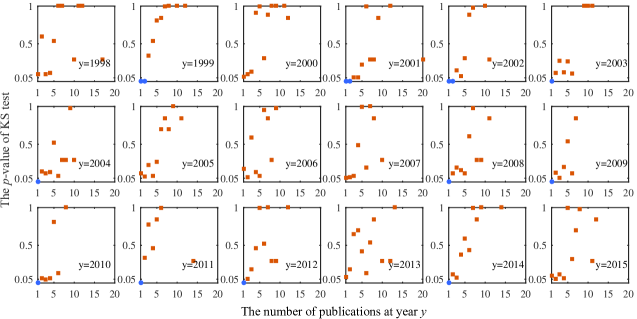
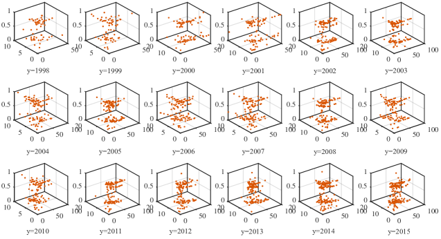
First, we showed the reasonability of modifying $(\zeta_{mj})_{M\times J}$. We partitioned the researchers of the training dataset into subsets according to their number of publications in a given year. The Kolmogorov-Smirnov (KS) test rejected the null hypothesis that the coauthor distributions of some large subsets (with 1 or 2 annual publications) are Poisson distributions (Fig. 1). Diminishing the diversity in researchers’ historical number of coauthors reveals the Poisson character of the coauthor distributions. The KS test cannot reject the null hypothesis that the coauthor distributions of researchers with the same annual number of publications and historical number of coauthors are Poisson distributions (Fig. 2). Therefore, it is necessary to modify $(\zeta_{mj})_{M\times J}$ to express the cumulative advantage of the historical number of coauthors, which gives the reasonability of the formulae in Eq. (7).

Figure 1: The $p$-value of the KS test with the hypothesis that a random variable follows a Poisson distribution. The panels show the results of the KS test on the number of coauthors of a researcher with $m$ publications in year $y$, where $m=1,...,20$. If the $p$-value$\leq 0.05$, the test rejects the hypothesis (blue circles); otherwise, it cannot reject the hypothesis (red squares).

Figure 2: Eliminating the diversities in the historical number of coauthors and the annual number of publications induces Poisson distributions. Consider the researchers with $m$ publications (upper right direction) in year $y$ and with $l$ coauthors before $y$ (upper left direction). If the $p$-value$\leq 0.05$ (vertical direction), the KS test rejects the hypothesis that the number of coauthors of that researcher follows a Poisson distribution (blue squares); otherwise, it cannot reject the hypothesis (red circles).

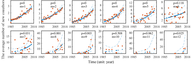
Secondly, we showed the significance of the regression results on the training dataset. The $\chi^{2}$ test indicates that $\eta_{ij}$ significantly correlates to $i$ given $j$, and to $j$ given ${i}$[45]. The $\chi^{2}$ test indicates that $\xi_{mj}$ significantly correlates to $t_{j}$ given $m$ from $1$ to $9$ except $6$ (see the $p$-value in Fig. 3). The researchers with that $m$ account for $99.68\%$ of the researchers in the training dataset. These significant correlations guarantee the effectiveness of utilizing regression methods to calculate $(\lambda_{ij})_{I\times J}$ and $(\zeta_{mj})_{M\times J}$.

Figure 3: The relationship between $\xi_{mj}$ and $t_{j}$ given $m$. Consider the researchers with $m$ publications at $(t_{j-1},t_{j}]$. The panels show the average number of new coauthors of these researchers at $(t_{j-1},t_{j}]$ ($\xi_{mj}$, red squares), the predicted results by the Poisson regression ($\zeta_{mj}$, blue dots), and the confidence intervals of the regression (dashed lines). When $p<0.05$, the $\chi^{2}$ test rejects the null hypothesis that the regression coefficient of time is equal to zero.

Evolutionary trend of the number of coauthors

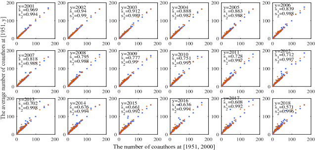
Consider the tested researchers who have $k$ coauthors at the time interval $[T_{0},t_{X}]$. Let $n(k,t_{j})$ be the average number of these researchers’ new coauthors arriving at the time interval $(t_{j-1},t_{j}]$, and $m(k,t_{j})$ be that predicted by the model. Fig. 4 shows the trends of $n(k,t_{j})$ and $m(k,t_{j})$ on $k$ at each year $t_{j}$ from $2001$ to $2018$.

The correlation of the trends is measured by the Pearson correlation coefficient[52] on individual level ($s_{1}$: calculated based on the list of researchers’ number of coauthors and that of their predicted one) and that on group level ($s_{2}$: sort the lists, and then calculate the coefficient). The value of $s_{1}$ decreases over time, whereas that of $s_{2}$ keeps high. It indicates that the model is unapplicable to the long-time prediction for individuals, but can be applicable for a group of researchers.

Figure 4: Fittings on the evolution of the number of researchers’ coauthors. Consider the tested researchers who have $k$ coauthors at $[1951,2000]$, where $k=1,...,200$. The panels show the average number of coauthors of these researchers at $[1951,y]$ ($n(k,y)$, red dots) and the predicted number ($m(k,y)$, blue lines). Index $s_{1}$ is the Pearson correlation coefficient calculated based on the list of researchers’ number of coauthors and their predicted number. Index $s_{2}$ is this coefficient based on the sorted lists.

Coauthor distributions

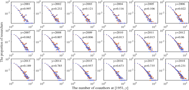
We compared the coauthor distribution of the tested researchers at $[T_{0},y]$ with the predicted distribution, where $y=2001,...,2018$. Fig. 5 shows that a fat tail emerges in the evolution of the ground-truth distribution and in that of the predicted distribution. This shows that our model can capture the fat-tail phenomenon. The KS test rejects that some of the compared distributions are the same (see the $p$-value in Fig. 5), although there is a coincidence in their heads. This indicates that the prediction precision for researchers with many coauthors needs to be improved.

Figure 5: Fittings on coauthor distributions. The panels show the coauthor distribution of the tested researchers at time interval $[1951,y]$ (red circles) and the predicted distribution (blue squares). When $p>0.05$, the KS test cannot reject the null hypothesis that the two distributions are the same.

Collaboration events

The above two experiments focus on the prediction precision of our model over a long time interval. The following experiment is designed to test the precision over a short time interval, namely, the next year. The model can provide the probability of the researcher $s$ having new coauthors in the next time interval $(t_{l-1},t_{l}]$:

$$p_{s}(t_{l})=1-\mathrm{e}^{-\lambda_{h_{s}(t_{l-1})t_{l}}}-\sum^{M}_{x=1}\frac{x^{\lambda_{h_{s}(t_{l-1})t_{l}}}}{x!}\mathrm{e}^{-\lambda_{h_{s}(t_{l-1})t_{l}}}\mathrm{e}^{-(\tilde{\zeta}_{xt_{l}})_{s}}.$$ (8)

The area under the curve (AUC) of the receiver operating characteristic is used to measure the prediction precision. Count the times that a researcher did (did not) collaborate with new coauthors in the next time interval, the probability is larger (smaller) than 0.5. Denote the counts by $m_{1}$ and $m_{2}$ respectively. Count the times that the probability is 0.5, and denote the count by $m_{3}$. Denote the number of tested researchers by $m$. Then,

$$\mathrm{AUC}=\frac{m_{1}+m_{2}+0.5m_{3}}{m}.$$ (9)

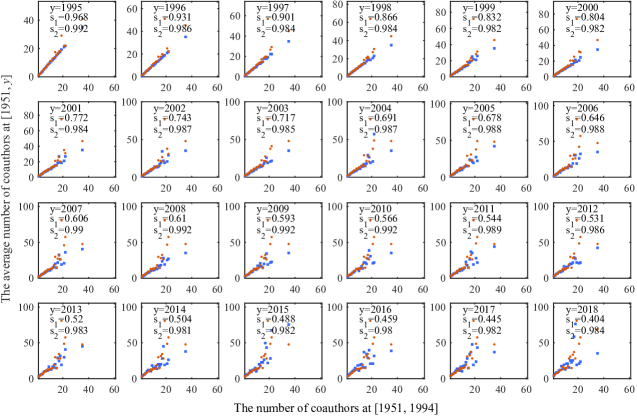
Fig. 6 shows that the AUC value is high for researchers with a small historical number of publications. This indicates that the model can provide a satisfactory prediction for the collaboration events of researchers with low productivity. It also indicates that there is no regularity of collaborations that can be revealed by our model for highly productive researchers, which indicates a direction for improving of the model. Due to the vast number of low productivity researchers, the AUC value is high for all of the tested researchers.

Figure 6: The precision of predicting collaboration events. The red dots show the AUC of predicting the collaboration events at year $y$ for the tested researchers who produced $i$ publications at $[1951,y-1]$, where $i=1,...,50$. The index AUC is calculated based on all of the tested researchers.

Discussion and conclusions

A learning model is proposed to predict the number of coauthors for researchers. Its practicability is tested on the dblp dataset, and its effectiveness is exhibited by the satisfactory fittings on the evolutionary trend of the number of coauthors for researchers, the distribution of this variable, and the occurrence probability of collaboration events. Note that our model cannot provide an exact prediction for an individual. However, due to its nature of regression, it can still be of use in its ability to provide a satisfactory prediction for a group of randomly selected researchers on average.

The parameters of our model are learned from a training dataset, the methods of which can be generalized to determine the parameters for models of coauthorship networks or other network models. The hyperparameters of our model are used to modify the intermediate results given by regression. The formulae of modification express the cumulative advantage of attracting coauthors on the historical number of coauthors, which enables our model to directly predict the number of coauthors generated by an inhomogeneous Poisson process.

The model provides a platform to utilize multiple factors by substituting them in the right side of Eqs. (2,4,6). A limitation of the results is that only three factors are used, namely, time, the historical number of publications, and the historical number of coauthors. Analyzing massive data to track the scientific careers of researchers would help to advance our understanding of how collaboration patterns evolve. The career stage of a researcher is worth considering as an influencing factor. It would be interesting to input the rank of the institutions to which researchers belong, the number of affiliations of past coauthors, the academic age, and reputation of researchers.

Appendix A: Evidence to support the motivation

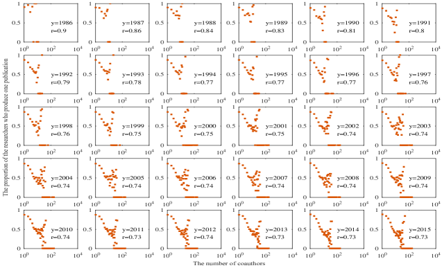
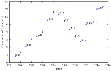
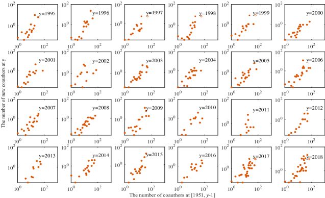
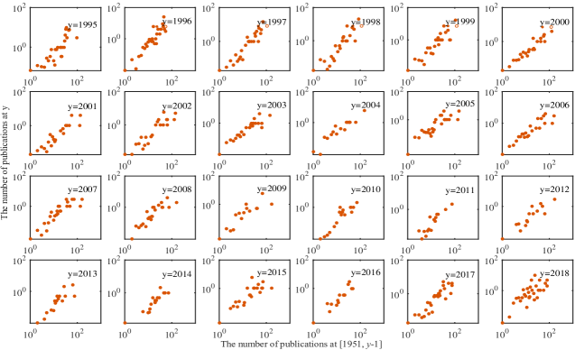
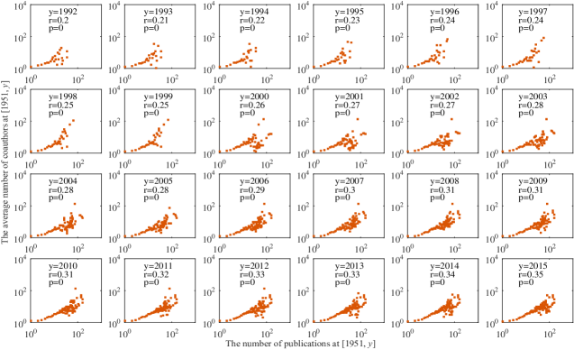
Fig. 7 shows the proportion of researchers who produced only one publication in the considered dataset. The sample size influences the $p$-value of the KS test[54]: it can be larger than $0.05$ in a large sample and smaller than $0.05$ in a small sample. Fig. 8 shows that the sample sizes of the tests shown in Fig. 2 are not very large. Fig. 9 shows the cumulative advantage of attracting new coauthors on researchers’ historical number of coauthors. Fig. 10 shows the cumulative advantage of producing new publications on researchers’ historical number of coauthors. Fig. 11 shows the positive correlation between the number of publications of a researcher and his or her number of coauthors.

Figure 7: The proportion of researchers who produced only one publication in the considered dataset. The panels show that the proportion $r$ is more than 70% in each year.

Figure 8: The largest sample size of the KS test shown in Fig. 2 for each year. The panel shows the size of the largest group of researchers with $m$ publications at year $y$ and with $l$ coauthors at $[1951,y-1]$ for any possible $(m,l)$.

Figure 9: The cumulative advantage of attracting new coauthors. The panels show the average number of new coauthors appearing in year $y$ of researchers whose number of coauthors at $[1951,y-1]$ are the same.

Figure 10: The cumulative advantage of producing publications. The panels show the average number of publications in year $y$ of researchers whose number of publications at $[1951,y-1]$ are the same.

Figure 11: The correlation between the number of publications and the number of coauthors. Consider the researchers who produced publications at $[1951,y]$, where $y=1992,...,2005$. The panels show the average number of coauthors at $[1951,y]$ of researchers who have the same number of publications at $[1951,y]$. The Spearman correlation coefficient $r$ is significantly larger than $0$, $p$-value$<0.05$.

Appendix B: The inapplicability of autoregressive models

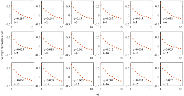
In statistics, autoregressive models specify that the response variable depends linearly on its previous values with a stochastic term. The advantage of those models is that they do not require much information; only the self-variable series is needed. If the autocorrelation coefficients of the response variable series are smaller than 0.5, then autoregressive models are not suitable for the prediction task. The autocorrelation coefficient of ${\boldsymbol{y}}=(y_{1},...,y_{T})$ with lag $l$ is defined as

$$r_{l}=\frac{\sum^{T-l}_{t=1}(y_{t}-\bar{\boldsymbol{y}})(y_{t+l}-\bar{\boldsymbol{y}})}{\sum^{T}_{t=1}(y_{t}-\bar{\boldsymbol{y}})^{2}},$$ (10)

where $l<T$, and $\bar{\boldsymbol{y}}$ is the mean of ${\boldsymbol{y}}$’s elements[53].

Consider a researcher $s$ in test dataset Set 4. Consider his or her series of the number of coauthors ${\boldsymbol{k}}_{s}=(k_{s}(t_{U}),...,k_{s}(t_{V}))$, where $k_{s}(t_{l})$ is his or her number of coauthors at $[T_{0},t_{l}]$ for $t_{U}\leq t_{l}\leq t_{V}$. Substitute the series into Eq. (10), and calculate the autocorrelation coefficients. Fig. 12 shows that these coefficients with a lag $>1$ are almost all smaller than 0.5. Therefore, an individual’s historical number of coauthors is not sufficient to predict his or her future number of coauthors. This finding indicates that the autoregressive models may not be suitable for the prediction of the number of coauthors.

Figure 12: Autocorrelation coefficients of the time series on the cumulative number of coauthors. Let $k_{s}(t_{j})$ be the number of coauthors of researcher $s$ at time interval $[1951,t_{j}]$. Consider the time series ${k}_{s}=(k_{s}(t_{X}),...,k_{s}(t_{Z}))$, where $t_{X}=2000$, and $t_{Z}=2018$. The panels show the average autocorrelation coefficients of this time series over the group of researchers in Set 4 who have $i$ coauthors at $[1951,2000]$. Index $q$ is group proportion.

Appendix C: An other example

The training and validation datasets here are Sets 5 and 6. The parameters of the test dataset (Set 3) are $t_{X}=1994$, $t_{Y}=2010$, and $t_{Z}=2018$. We only predicted the publications for 99.98% of the researchers in Set 3 who have no more than $60$ publications at the time interval $[T_{0},t_{X}]$ and no more than $12$ annual publications at $[t_{X},t_{Z}]$. Figs. 13-15 show the prediction results of our model.

Figure 13: Fittings on the evolution of the number of coauthors for researchers. Consider the tested researchers who have $k$ coauthors at $[1951,1994]$, where $k=1,...,60$. The panels show the average number of coauthors for these researchers at $[1951,y]$ ($n(k,y)$, red dots) and the predicted number ($m(k,y)$, blue lines). Index $s_{1}$ is the Pearson correlation coefficient calculated based on the list of researchers’ number of coauthors and the list of their predicted number. Index $s_{2}$ is this coefficient based on the sorted lists.

Figure 14: Fittings on coauthor distributions. The panels show the coauthor distribution of the tested researchers at time interval $[1951,y]$ (red circles) and the predicted one (blue squares). When $p>0.05$, the KS test cannot reject the hypothesis that the compared distributions are the same.

Figure 15: The precision of predicting collaboration events. The red dots show the AUC of predicting the collaboration events at year $y$ for the tested researchers who produced $i$ publications at $[1951,y-1]$, where $i=1,...,50$. Index AUC is calculated based on all of the tested researchers.

References

- 1. Committee on the Science of Team Science. Enhancing the Effectiveness of Team Science (National Academies Press, Washington DC, 2015).
- 2. Corrêa JREA, Silva FN, Costa LDF, Amancio DR (2017) Patterns of authors contribution in scientific manuscripts. J Informetr, 11(2), 498-510.
- 3. Lu C, Zhang Y, Ahn YY, Ding Y, Zhang C, Ma D (2019). Co-contributorship network and division of labor in individual scientific collaborations. J Assoc Inf Sci Technol, DOI: 10.1002/asi.24321.
- 4. Li F, Miao Y, Yang C (2015) How do alumni faculty behave in research collaboration? An analysis of Chang Jiang Scholars in China. Res Policy, 44(2), 438-450.
- 5. Moody J (2004) The strucutre of a social science collaboration network: disciplinery cohesion form 1963 to 1999. Am Sociol Rev, 69(2): 213-238.
- 6. Xie Z, Li M, Li JP, Duan XJ, Ouyang ZZ (2018) Feature analysis of multidisciplinary scientific collaboration patterns based on PNAS. EPJ Data Science, 7: 5.
- 7. Wagner CS, Leydesdorff L (2005) Network structure, self-organization, and the growth of international collaboration in science. Res Policy, 34(10): 1608-1618.
- 8. Katz JS (1994) Geographical proximity and scientific collaboration. Scientometrics, 31(1), 31-43.
- 9. Perc C (2010) Growth and structure of Slovenia’s scientific collaboration network. J Informetr, 4: 475-482.
- 10. Leclerc M, Gagné J (1994) International scientific cooperation: The continentalization of science. Scientometrics, 31(3), 261-292.
- 11. Russell JM (1995) The increasing role of international cooperation in science and technology research in Mexico. Scientometrics, 34(1), 45-61.
- 12. Glänzel W, Schubert A, Czerwon HJ (1999) A bibliometric analysis of international scientific cooperation of the European Union (1985-1995). Scientometrics, 45(2), 185-202.
- 13. Gomez I, Fernández MT, Sebastian J (1999) Analysis of the structure of international scientific cooperation networks through bibliometric indicators. Scientometrics, 44(3), 441-457.
- 14. Narin F, Stevens K, Whitlow ES (1991) Scientific co-operation in Europe and the citation of multinationally authored papers. Scientometrics, 21(3), 313-323.
- 15. Khor KA, Yu LG (2016) Influence of international co-authorship on the research citation impact of young universities. Scientometrics, 107(3), 1095-1110.
- 16. Wuchty S, Jones BF, Uzzi B (2007) The increasing dominance of teams in production of knowledge. Science, 316(5827), 1036-1039.
- 17. Valderas JM (2007) Why do team-authored papers get cited more?. Science, 317(5844), 1496-1498.
- 18. Vogel AL, Stipelman BA, Hall KL, Nebeling L, Stokols D, Spruijt-Metz D (2014) Pioneering the transdisciplinary team science approach: Lessons learned from National Cancer Institute grantees. J Tran Med Epid, 2(2).
- 19. Hall KL, Stokols D, Stipelman BA, Vogel AL, Feng A, Masimore B et al (2012). Assessing the value of team science: a study comparing center-and investigator-initiated grants. Am J Prev Med 42(2), 157-163.
- 20. Uzzi B, Mukherjee S, Stringer M, Jones B (2013) Atypical combinations and scientific impact. Science, 342(6157), 468-472.
- 21. Wu L, Wang D, Evans JA (2019) Large teams develop and small teams disrupt science and technology. Nature, 566, 378-382.
- 22. Newman M (2004) Coauthorship networks and patterns of scientific collaboration. Proc Natl Acad Sci USA, 101: 5200-5205.
- 23. Guimerá R, Uzzi B, Spiro J, Amaral LAN (2005) Team assembly mechanisms determine collaboration network structure and team performance. Science, 308, 697-702.
- 24. Barabási AL, Jeong H, Néda Z, Ravasz E, Schubert A, Vicsek T (2002) Evolution of the social network of scientific collaborations. Physica A, 311(3-4), 590-614.
- 25. Xie Z, Ouyang ZZ, Li JP (2016) A geometric graph model for coauthorship networks. J Informetr, 10: 299-311.
- 26. Xie Z, Xie ZL, Li M, Li JP, Yi DY (2017) Modeling the coevolution between citations and coauthorship of scientific papers. Scientometrics, 112: 483-507.
- 27. Newman M (2001) Scientific collaboration networks. I. network construction and fundamental results. Phys Rev E, 64: 016131.
- 28. Newman M (2001) Scientific collaboration networks. II. shortest paths, weighted networks, and centrality. Phys Rev E, 64: 016132.
- 29. Newman M (2001) The structure of scientific collaboration networks. Proc Natl Acad Sci USA, 98: 404-409.
- 30. Newman M (2001) Clustering and preferential attachment in growing networks. Phys Rev E, 64(2): 025102.
- 31. Newman M (2002) Assortative mixing in networks. Phys Rev Lett, 89: 208701.
- 32. Zhang C, Bu Y, Ding Y, Xu J (2018) Understanding scientific collaboration: Homophily, transitivity, and preferential attachment. J Assoc Inf Sci Technol, 69(1), 72-86.
- 33. Amancio DR, Oliveira Jr, ON, Costa LDF (2012) On the use of topological features and hierarchical characterization for disambiguating names in collaborative networks. Europhys Lett, 99(4), 48002.
- 34. Santos FC, Pacheco JM (2005) Scale-free networks provide a unifying framework for the emergence of cooperation. Phys Rev Lett, 95(9): 098104.
- 35. Perc M (2014) The Matthew effect in empirical data. J R Soc Interface, 11: 20140378.
- 36. Xie Z, Li JP, Li M (2018) Exploring cooperative game mechanisms of scientific coauthorship networks. Complexity, 9173186.
- 37. Hunter L, Leahey E (2008) Collaborative research in sociology: trends and contributing factors. Am Sociol, 39, 290-306.
- 38. Melin, G. (2000) Pragmatism and self-organization: Research collaboration on the individual level. Research policy, 29(1), 31-40.
- 39. Hoekman J, Frenken K, Tijssen RJ (2010) Research collaboration at a distance: Changing spatial patterns of scientific collaboration within Europe. Research policy, 39(5), 662-673.
- 40. Van Rijnsoever FJ, Hessels LK (2011) Factors associated with disciplinary and interdisciplinary research collaboration. Research policy, 40(3), 463-472.
- 41. Qi M, Zeng A, Li M, Fan Y, Di Z (2017) Standing on the shoulders of giants: the effect of outstanding scientists on young collaborators’ careers. Scientometrics, 111(3), 1839-1850.
- 42. Jones BF, Wuchty S, Uzzi B (2008) Multi-university research teams: shifting impact, geography, and stratification in science. Science, 322, 1259-1262.
- 43. Xie Z (2019) A cooperative game model for the multimodality of coauthorship networks, Scientometrics, 121(1), 503-519.
- 44. Xie Z (2019) Predicting publication productivity for researchers: a piecewise Poisson model. arXiv:1908.07564.
- 45. Xie Z (2019) Predicting publication productivity for researchers: a latent variable model, arxiv:1910.02507.
- 46. Lee S, Bozeman B (2005) The impact of research collaboration on scientific productivity. Soc Stud Sci 35: 673-702.
- 47. Ductor L (2015) Does co-authorship lead to higher academic productivity? Oxford B Econ Stat, 77(3), 385-407.
- 48. Consul PC, Jain GC (1973) A generalization of the Poisson distribution. Technometrics, 15(4), 791-799.
- 49. Lotka AJ (1926) The frequency distribution of scientific productivity. J Wash Acad Sci, 16(12), 317-323.
- 50. Xie Z, Ouyang ZZ, Li JP, Dong EM, Yi DY (2018) Modelling transition phenomena of scientific coauthorship networks. J Assoc Inf Sci Technol 69(2): 305-317.
- 51. Nelder JA, Wedderburn RW (1972) Generalized linear models. J R Stat Soc Ser A-G, 135(3), 370-384.
- 52. Hollander M, Wolfe DA (1973) Nonparametric Statistical Methods. Wiley.
- 53. Box GE, Jenkins GM, Reinsel GC, Ljung GM (2015) Time series analysis: forecasting and control. John Wiley & Sons.
- 54. Moore DS, McCabe GP, Craig BA (2014) Introduction to the Practice of Statistics. W. H. Freeman.