Self-Supervised Light Field Reconstruction Using Shearlet Transform and
Cycle Consistency

Abstract

The image-based rendering approach using Shearlet Transform (ST) is one of the state-of-the-art Densely-Sampled Light Field (DSLF) reconstruction methods. It reconstructs Epipolar-Plane Images (EPIs) in image domain via an iterative regularization algorithm restoring their coefficients in shearlet domain. Consequently, the ST method tends to be slow because of the time spent on domain transformations for dozens of iterations. To overcome this limitation, this letter proposes a novel self-supervised DSLF reconstruction method, CycleST, which applies ST and cycle consistency to DSLF reconstruction. Specifically, CycleST is composed of an encoder-decoder network and a residual learning strategy that restore the shearlet coefficients of densely-sampled EPIs using EPI reconstruction and cycle consistency losses. Besides, CycleST is a self-supervised approach that can be trained solely on Sparsely-Sampled Light Fields (SSLFs) with small disparity ranges ($\leqslant$ 8 pixels). Experimental results of DSLF reconstruction on SSLFs with large disparity ranges (16 - 32 pixels) from two challenging real-world light field datasets demonstrate the effectiveness and efficiency of the proposed CycleST method. Furthermore, CycleST achieves $\thicksim$ 9x speedup over ST, at least.

I Introduction

Densely-Sampled Light Field (DSLF) is a discrete 4D representation for the light rays from the scene encoded by two parallel planes, namely image plane and camera plane, where the disparity ranges between neighboring views are less or equal to one pixel. The DSLF has a wide range of applications, such as synthetic aperture imaging, depth estimation, segmentation and visual odometry [1]. Besides, the DSLF-based contents can be rendered on VR [2], 3DTV [3] and holographic [4] systems. A DSLF in real-world environment is extremely difficult to capture, due to the hardware limitations of the modern light field acquisition systems that can in most cases only capture Sparsely-Sampled Light Fields (SSLFs), where the disparity range between views is more than one pixel. Therefore, real-world DSLFs are typically reconstructed from real-world SSLFs using computational imaging approaches.

Related work. Video frame interpolation methods can be adapted to solve the DSLF reconstruction problem because a 3D SSLF can be treated as a virtual video sequence. Niklaus et al. have proposed Separable Convolution (SepConv), a learning-based video frame synthesis method using spatially adaptive kernels [5]. Bao et al. have proposed a Depth-Aware video frame INterpolation (DAIN) algorithm that leverages optical flow, local interpolation kernels, depth maps and contextual features [6]. Xu et al. have improved the linear models adopted in Liner Video Interpolation (LVI) methods [7, 8] and proposed the Quadratic Video Interpolation (QVI) approach considering the acceleration information in videos [9, 10, 11]. Gao and Koch were the first to extend SepConv for DSLF reconstruction by proposing Parallax-Interpolation Adaptive Separable Convolution (PIASC) [12]. More recently, Gao et al. have developed a learning-based DSLF reconstruction method, i.e. Deep Residual Shearlet Transform (DRST) [13], for coefficient restoration in the shearlet domain of densely-sampled Epipolar-Plane Images (EPIs) based on the conventional image-based rendering techniques [14, 15] using Shearlet Transform (ST) [16, 17, 18].

As for DSLF reconstruction on large-disparity-range (16 - 32 pixels) SSLFs of complex scenes, the aforementioned state-of-the-art video frame interpolation methods tend to fail. To tackle this problem, a novel self-supervised DSLF reconstruction method, CycleST, is proposed by leveraging shearlet transform and cycle consistency [19], also used by recent video frame interpolation methods [20, 21]. In particular, since several DSLFs with different angular resolutions can be reconstructed from the same input SSLF, the cycle consistency is the technique that guarantees these DSLFs have similar reconstruction results w.r.t. the same angular positions.

We summarize the main contributions of this letter as below:

• The proposed CycleST fully leverages the deep convolutional network with cycle consistency loss in shearlet domain to perform EPI inpainting in image domain.

• CycleST is fully self-supervised and trained solely on synthetic SSLFs with small disparity ranges ($\leqslant$ 8 pixels);

• Experimental results on challenging real-world SSLFs with large disparity ranges (16 - 32 pixels) demonstrate the superiority of CycleST over ST for DSLF reconstruction in terms of accuracy and efficiency ($>$ 8.9x speedup).

II Methodology

II-A Preliminaries

II-A1 Symbols and notations

The symbols and notations used by this letter are elaborated in Table I. As can be seen in the table, the target DSLF $\mathcal{D}$ to be reconstructed from the input SSLF $\mathcal{S}$ has the same spatial resolution ($m\times l$) but different angular resolutions. Specifically, on the one hand, the angular resolution of $\mathcal{D}$, i.e. $\dot{n}$, is dependent on that of $\mathcal{S}$, i.e. $n$, and the sampling interval $\tau$ specified by the user such that $\dot{n}=\big{(}(n-1)\tau+1\big{)}$. On the other hand, $\tau$ relies on the disparity range $d_{\mathrm{range}}^{\mathcal{S}}$ of $\mathcal{S}$, i.e. $\tau\geqslant d_{\mathrm{range}}^{\mathcal{S}}$. Since this paper aims to enhance the angular resolution of any input $\mathcal{S}$ with large disparity ranges ($16<d_{\mathrm{range}}^{\mathcal{S}}\leqslant 32$ pixels), we fix $\tau$ to 32. Both $\mathcal{S}$ and $\mathcal{D}$ can be regarded as sets of EPIs, i.e. $\mathcal{S}=\{\varepsilon_{i}|1\leqslant i\leqslant l\}$ and $\mathcal{D}=\{\zeta_{i}|1\leqslant i\leqslant l\}$. It is obvious that $\varepsilon_{i}$ and $\zeta_{i}$ have different heights because of the different angular resolutions. Due to the lack of DSLF datasets, in this letter for the CycleST network training we utilize the available community-supported SSLF datasets with small disparity ranges ($\leqslant$ 8 pixels). Let $\mathcal{S}^{\prime}=\{\epsilon_{i}|1\leqslant i\leqslant l\}$ denote one of these training SSLFs, where $d_{\mathrm{range}}^{\mathcal{S}^{\prime}}\leqslant 8$ pixels and $\epsilon_{i}\in\mathbb{R}^{m\times n^{\prime}\times 3}$. The sampling interval from $\mathcal{D}$ to $\mathcal{S}^{\prime}$ is represented by $\tau^{\prime}$, where $\tau^{\prime}\geqslant d_{\mathrm{range}}^{\mathcal{S}^{\prime}}$. Here, we fix $\tau^{\prime}$ to 8. This letter studies how to reconstruct densely-sampled $\mathcal{D}$ from large-disparity-range $\mathcal{S}$ using a deep neural network trained solely on small-disparity-range $\mathcal{S}^{\prime}$ in a self-supervised fashion.

Table I: Symbols and notations.

Symbol	Name	Description
$m\times l$	Spatial resolution of $\mathcal{S}$, $\mathcal{S}^{\prime}$ and $\mathcal{D}$	width $\times$ height
$n$, $n^{\prime}$, $\dot{n}$	Angular resolutions of $\mathcal{S}$, $\mathcal{S}^{\prime}$ and $\mathcal{D}$
$\varepsilon_{i}$	Sparsely-sampled EPI (SSEPI)	$\varepsilon_{i}\in\mathbb{R}^{m\times n\times 3}$
$\epsilon_{i}$	SSEPI (for training)	$\epsilon_{i}\in\mathbb{R}^{m\times n^{\prime}\times 3}$
$\zeta_{i}$	Densely-sampled EPI	$\zeta_{i}\in\mathbb{R}^{m\times\dot{n}\times 3}$
$\mathcal{S}$	Large-disparity-range SSLF	$\mathcal{S}=\{\varepsilon_{i}|1\leqslant i\leqslant l\}$
	($16<\mathrm{disp}(\mathcal{S})\leqslant 32$ pixels)
$\mathcal{S}^{\prime}$	Small-disparity-range SSLF (for training)	$\mathcal{S}^{\prime}=\{\epsilon_{i}|1\leqslant i\leqslant l\}$
	($1<\mathrm{disp}(\mathcal{S}^{\prime})\leqslant 8$ pixels)
$\mathcal{D}$	Target DSLF to be reconstructed from $\mathcal{S}$	$\mathcal{D}=\{\zeta_{i}|1\leqslant i\leqslant l\}$
	($\mathrm{disp}(\mathcal{D})\leqslant 1$ pixel)
$d_{\min}^{\mathcal{S}}$	Minimum disparity of $\mathcal{S}$	$d_{\min}^{\mathcal{S}}=\mathrm{min}\big{(}\mathrm{disp}(\mathcal{S})\big{)}$
$d_{\max}^{\mathcal{S}}$	Maximum disparity of $\mathcal{S}$	$d_{\max}^{\mathcal{S}}=\mathrm{max}\big{(}\mathrm{disp}(\mathcal{S})\big{)}$
$d_{\mathrm{range}}^{\mathcal{S}}$	Disparity range of $\mathcal{S}$	$d_{\mathrm{range}}^{\mathcal{S}}=\big{(}d_{\max}^{\mathcal{S}}-d_{\min}^{\mathcal{S}}\big{)}$
$\tau$	Sampling interval ($\mathcal{D}\rightarrow\mathcal{S}$)	$\tau=\frac{\dot{n}-1}{n-1}=32$
$\tau^{\prime}$	Sampling interval ($\mathcal{D}\rightarrow\mathcal{S}^{\prime}$)	$\tau^{\prime}=\frac{\dot{n}-1}{n^{\prime}-1}=8$

II-A2 Shearlet Transform (ST)

ST is originally proposed in [22, 23, 24] and extended by Vagharshakyan et al. for DSLF reconstruction [16, 17, 18], where an elaborately-tailored shearlet system with $\xi$ scales is developed for the angular resolution enhancement of any input $\mathcal{S}$ with two requirements: (i) $d_{\min}^{\mathcal{S}}\geqslant 0$ and (ii) $d_{\max}^{\mathcal{S}}\leqslant\tau$. The number of scales, i.e. $\xi$, is determined by the sampling interval $\tau$ as $\xi={\lceil\log_{2}{\tau\rceil}}$. The constructed $\xi$-scale shearlet system is used by shearlet analysis transform $\mathcal{SH}:\mathbb{R}^{\gamma\times\gamma}\rightarrow\mathbb{R}^{\gamma\times\gamma\times\eta}$ and shearlet synthesis transform $\mathcal{SH}^{*}:\mathbb{R}^{\gamma\times\gamma\times\eta}\rightarrow\mathbb{R}^{\gamma\times\gamma}$, where $\gamma\times\gamma$ represents the size of a shearlet filter and $\eta=(2^{\xi+1}+\xi-1)$ denotes the number of shearlets. For $\tau=32$, $\xi=5$ and $\eta=68$. Moreover, as suggested in [16], for $\tau=32$, a good choice for $\gamma$ is $\gamma=255$.

II-B CycleST

To resolve the challenging DSLF reconstruction problem for large-disparity-range SSLFs using small-disparity-range SSLF data only, we propose a novel self-supervised method that leverages a residual learning-based convolutional network with EPI reconstruction and cycle consistency losses to restore EPI coefficients in shearlet domain. The proposed approach is referred to as CycleST and consists of five steps, namely (i) pre-shearing, (ii) random cropping, (iii) remapping, (iv) sparse regularization and (v) post-shearing. It is worth remarking that steps (i), (ii), (iii) and (iv) belong to the self-supervised training part of CycleST and steps (i), (iii), (iv) and (v) constitute the prediction part of CycleST. The details of these five steps are described as following.

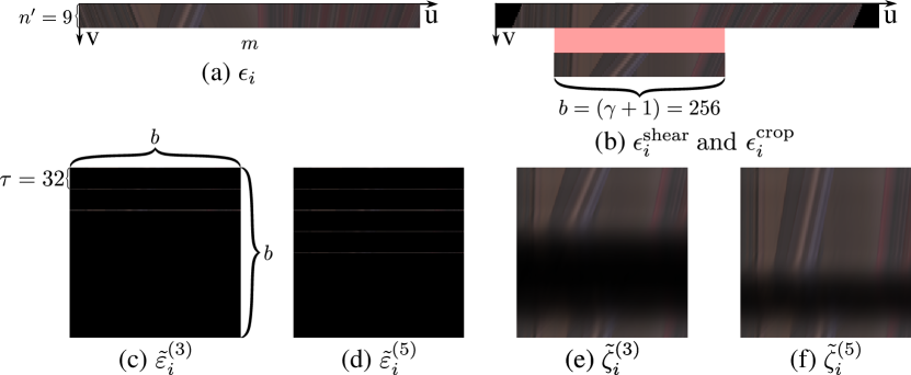
Figure 1: Illustration of the preparation of training data for CycleST. An EPI $\epsilon_{i}$ of the training SSLF $\mathcal{S}^{\prime}$ is presented in (a). In (b), the top row shows $\epsilon^{\mathrm{shear}}_{i}$, i.e. the result of the pre-shearing operation on $\epsilon_{i}$, and the bottom row shows $\epsilon^{\mathrm{crop}}_{i}$, which is the result of the random cropping step on $\epsilon^{\mathrm{shear}}_{i}$. The remapped EPIs $\tilde{\varepsilon}_{i}^{(3)}$ and $\tilde{\varepsilon}_{i}^{(5)}$ from $\epsilon^{\mathrm{crop}}_{i}$ are exhibited in (c) and (d), respectively. The corresponding reconstruction results of the sparse regularization step, i.e. $\tilde{\zeta}_{i}^{(3)}$ and $\tilde{\zeta}_{i}^{(5)}$, are displayed in (e) and (f), respectively.

II-B1 Pre-shearing

To satisfy the two requirements of the elaborately-tailored shearlet system explained in Section II-A2, a pre-shearing operation is designed to change the disparities of the input training SSLF $\mathcal{S}^{\prime}$ using a shearing parameter $\rho^{\mathcal{S}^{\prime}}$, where $\Big{(}d_{\min}^{\mathcal{S}^{\prime}}-\big{(}\tau^{\prime}-d_{\mathrm{range}}^{\mathcal{S}^{\prime}}\big{)}\Big{)}\leqslant\rho^{\mathcal{S}^{\prime}}\leqslant d_{\min}^{\mathcal{S}^{\prime}}$. To be precise, each row $v$ of $\epsilon_{i}$ is sheared by $(n^{\prime}-v)\rho^{\mathcal{S}^{\prime}}$ pixels, where $1\leqslant v\leqslant n^{\prime}$. One of the EPIs of the training SSLF $\mathcal{S}^{\prime}$, i.e. $\epsilon_{i}$, is displayed in Fig. 1 (a). The sheared $\epsilon_{i}$ is represented by $\epsilon^{\mathrm{shear}}_{i}$ as illustrated in Fig. 1 (b).

II-B2 Random cropping

To augment the number of training samples, a random cropping operation is leveraged to randomly cut an EPI $\epsilon_{i}^{\mathrm{crop}}$ from the above generated $\epsilon^{\mathrm{shear}}_{i}$ with a smaller width $b=(\gamma+1)=256$ pixels. Note that this operation does not crop any black border region of $\epsilon^{\mathrm{shear}}_{i}$. An example of the random cropping results is shown in Fig. 1 (b).

II-B3 Remapping

To achieve self-supervision for CycleST, the rows of the cropped EPI $\epsilon_{i}^{\mathrm{crop}}$ are rearranged with zero-padding between neighboring rows, producing EPIs $\tilde{\varepsilon}_{i}^{(t)}$, i.e.

$$\tilde{\varepsilon}_{i}^{(t)}\Big{(}1:\tau:\big{(}(t-1)\tau+1\big{)}\Big{)}=\epsilon_{i}^{\mathrm{crop}}\Big{(}1:\tfrac{n^{\prime}-1}{t-1}:n^{\prime}\Big{)}\,,$$ (1)

where $\tilde{\varepsilon}_{i}^{(t)}\in\mathbb{R}^{b\times b\times 3}$. As shown in Fig. 1 (c) and (d), two different EPIs, i.e. $\tilde{\varepsilon}_{i}^{(3)}$ and $\tilde{\varepsilon}_{i}^{(5)}$, are generated for each $\epsilon_{i}^{\mathrm{crop}}$, so that the cycle consistency information from them can be leveraged in the next sparse regularization step.

Figure 2: Architecture of the deep convolutional network of CycleST, referred to as $\mathcal{R}(\cdot)$. Based on the U-Net architecture [25] and residual learning strategy [26], $\mathcal{R}(\cdot)$ refines the shearlet coefficients of $\tilde{\varepsilon}_{i}^{(t)}$ in shearlet domain to produce inpainted $\tilde{\zeta}_{i}^{(t)}$ in image domain.

II-B4 Sparse regularization

The remapped EPI $\tilde{\varepsilon}_{i}^{(t)}$ is then converted into shearlet coefficients via the shearlet analysis transform $\mathcal{SH}(\cdot)$. The sparse regularization step is essentially refining these coefficients in shearlet domain to fulfill image inpainting on $\tilde{\varepsilon}_{i}^{(t)}$ in image domain. To this end, the state-of-the-art deep learning techniques are exploited. In particular, a deep network using cycle consistency loss with self-supervision setup is designed for the reconstruction of the shearlet coefficients. The details of the network architecture and loss function of CycleST network are described as below.

Network architecture. As shown in Fig. 2, a residual convolutional network, based on the architectures of U-Net [25] and the generator network of CycleGAN [19], is adapted to perform the reconstruction of shearlet coefficients. The input data are $\tilde{\varepsilon}_{i}^{(t)}$, $t\in\{3,5\}$, in image domain, which can be converted into coefficients $\mathcal{SH}\Big{(}\tilde{\varepsilon}_{i}^{(t)}\Big{)}$ with $\eta=68$ channels in shearlet domain. These coefficients are then fed to the encoder-decoder network of CycleST, represented by $\mathcal{R}(\cdot)$, to predict the residuals for the input coefficients, i.e. $\mathcal{R}\Big{(}\mathcal{SH}\big{(}\tilde{\varepsilon}_{i}^{(t)}\big{)}\Big{)}$. The encoder component of $\mathcal{R}(\cdot)$ has four hierarchies, of which each is composed of one $3\times 3$ convolution, one Leaky ReLU and one average pooling layers. The decoder part also has four hierarchies. Each one consists of the same convolution and Leaky ReLU layers as that of the encoder, but a bilinear upsampling layer instead of the pooling layer. The skip connections concatenate the outputs of last three hierarchies of both encoder and decoder. It can also be seen that the last layer of $\mathcal{R}(\cdot)$ is only a $1\times 1$ convolution layer, without Leaky ReLU placed behind it. Following the residual learning strategy [26], the predicted coefficient residuals $\mathcal{R}\Big{(}\mathcal{SH}\big{(}\tilde{\varepsilon}_{i}^{(t)}\big{)}\Big{)}$ are merged with $\mathcal{SH}\Big{(}\tilde{\varepsilon}_{i}^{(t)}\Big{)}$ via an element-wise addition operation. The output data of CycleST network are the corresponding densely-sampled EPIs $\tilde{\zeta}_{i}^{(t)}$, $t\in\{3,5\}$, which can be written as below:

$$\tilde{\zeta}_{i}^{(t)}=\mathcal{SH}^{*}\bigg{(}\mathcal{SH}\Big{(}\tilde{\varepsilon}_{i}^{(t)}\Big{)}+\mathcal{R}\Big{(}\mathcal{SH}\big{(}\tilde{\varepsilon}_{i}^{(t)}\big{)}\Big{)}\bigg{)}\,.$$ (2)

Loss function. Two kinds of losses are considered in the loss function of CycleST network, i.e. the EPI reconstruction loss $\mathcal{L}_{\mathrm{s}}(t)$ and cycle consistency loss $\mathcal{L}_{\mathrm{cyc}}$. Both of them employ $\ell_{1}$ norm, since recent research indicates that $\ell_{1}$ norm is superior over $\ell_{2}$ norm for learning-based view synthesis and image inpainting tasks [5, 27, 28]. The overall loss function $\mathcal{L}$ is a linear combination of $\mathcal{L}_{\mathrm{s}}(t)$, $t\in\{3,5\}$, and $\mathcal{L}_{\mathrm{cyc}}$, i.e.

$$\mathcal{L}=\mathcal{L}_{\mathrm{s}}(3)+\mathcal{L}_{\mathrm{s}}(5)+\lambda\mathcal{L}_{\mathrm{cyc}}\,.$$ (3)

The EPI reconstruction loss $\mathcal{L}_{\mathrm{s}}(t)$ measures the reconstruction errors between ground-truth sparsely-sampled $\epsilon_{i}^{\mathrm{crop}}$ and predicted densely-sampled $\tilde{\zeta}^{(t)}$ in a self-supervised manner:

$$\mathcal{L}_{\mathrm{s}}(t)=\left\lVert\tilde{\zeta}_{i}^{(t)}\Big{(}1:\tfrac{(t-1)\tau}{n^{\prime}-1}:\big{(}(t-1)\tau+1\big{)}\Big{)}-\epsilon_{i}^{\mathrm{crop}}\right\rVert_{1}.$$ (4)

The cycle consistency loss $\mathcal{L}_{\mathrm{cyc}}$ calculates the reconstruction differences between the predicted $\tilde{\zeta}^{(3)}$ and $\tilde{\zeta}^{(5)}$:

$$\mathcal{L}_{\mathrm{cyc}}=\left\lVert\tilde{\zeta}_{i}^{(3)}\Big{(}1:(2\tau+1)\Big{)}-\tilde{\zeta}_{i}^{(5)}\Big{(}1:2:(4\tau+1)\Big{)}\right\rVert_{1}.$$ (5)

Finally, $\lambda$ is empirically set to 2.

II-B5 Post-shearing

The post-shearing operation is only used in the inference phase of CycleST. In terms of using CycleST for reconstructing $\mathcal{D}$ from $\mathcal{S}$, the input $\mathcal{S}$ has been sheared with parameter $\rho^{\mathcal{S}}$ in the pre-shearing stage. The post-shearing step compensates this through the same shearing operation on $\tilde{\zeta}_{i}^{(n)}$ with a new shearing parameter $-\frac{\rho^{\mathcal{S}}}{\tau}$. The sheared $\tilde{\zeta}_{i}^{(n)}$ is then cut by only keeping the top $\big{(}(n-1)\tau+1\big{)}$ rows of it to produce $\zeta_{i}$ of the target $\mathcal{D}$. It is suggested that $\rho^{\mathcal{S}}=d_{\min}^{\mathcal{S}}$.

Table II: Details about the training and evaluation datasets.

3D light fields	$m$	$l$	$n^{\prime}$	$\ddot{n}$	$\delta$	n	$\dot{n}$
$\mathcal{S}^{\prime}_{j}$, $1\leqslant j\leqslant 78$	512	512	9	-	-	-	-
$\Psi^{1}_{j}$, $1\leqslant j\leqslant 9$	1280	720	-	97	16	7	193
$\Psi^{2}_{j}$, $j\in\{1,2\}$	960	720	-	97	16	7	193
$\Psi^{2}_{j}$, $j\in\{3,4\}$	960	720	-	97	32	4	97

III Experiments

III-A Experimental Settings

III-A1 Training dataset

The Inria synthetic light field datasets contains 39 synthetic 4D SSLFs with disparities from -4 to 4 pixels [29], satisfying the requirement $d_{\mathrm{range}}^{\mathcal{S}^{\prime}}\leqslant 8$ pixels in Section II-A1 for the training SSLF $\mathcal{S}^{\prime}$. These 4D SSLFs have the same angular resolution $9\times 9$ and spatial resolution $512\times 512$ pixels. We only pick the 5-th row and 5-th column 3D SSLFs from each synthetic 4D SSLF. Therefore, the training data of CycleST consists of $\mathcal{S}^{\prime}_{j}$, $1\leqslant j\leqslant 78$, $l=512$, $m=512$ and $n^{\prime}=9$. The pre-shearing operation in Section II-B1 is repeated three times for each $\mathcal{S}^{\prime}_{j}$ with different shearing parameters $\rho^{\mathcal{S}^{\prime}_{j}}\in\Big{\{}\Big{(}d_{\min}^{\mathcal{S}^{\prime}_{j}}-\big{(}\tau^{\prime}-d_{\mathrm{range}}^{\mathcal{S}^{\prime}_{j}}\big{)}\Big{)},\Big{(}d_{\min}^{\mathcal{S}^{\prime}_{j}}-0.5\cdot\big{(}\tau^{\prime}-d_{\mathrm{range}}^{\mathcal{S}^{\prime}_{j}}\big{)}\Big{)},d_{\min}^{\mathcal{S}^{\prime}_{j}}\Big{\}}$. As a result, the number of the generated $\epsilon^{\mathrm{crop}}_{i}$ for each training epoch is $78\times 3\times l=119,808$.

III-A2 Evaluation Datasets

Since there are few public real-world DSLF datasets, two evaluation datasets of light fields with tiny disparity ranges ($\leqslant$ 2 pixels) are considered for the performance evaluation of different DSLF reconstruction methods. The Evaluation Dataset 1 (ED1) is the tailored High Density Camera Array (HDCA) dataset [30] using the same cutting and scaling strategy as in [13]. Consequently, nine tiny-disparity-range light fields $\Psi^{1}_{j}$, $1\leqslant j\leqslant 9$, form ED1 with the same spatial resolution ($m\times l=1280\times 720$ pixels) and angular resolution ($\ddot{n}=97$). For each $\Psi^{1}_{j}$, an input SSLF $\mathcal{S}^{1}_{j}$ can be produced using an interpolation rate $\delta=16$. As a result, the angular resolution of $\mathcal{S}^{1}_{j}$ is $n=\big{(}\frac{\ddot{n}-1}{\delta}+1\big{)}=7$. The target $\mathcal{D}^{1}_{j}$ to be reconstructed from $\mathcal{S}^{1}_{j}$ has angular resolution $\dot{n}=193$. The MPI light field archive contains two tiny-disparity-range light fields (‘bikes’ and ‘workshop’) and two DSLFs (‘mannequin’ and ‘living room’) [31], which constitute the Evaluation Dataset 2 (ED2), i.e. $\Psi^{2}_{j}$, $1\leqslant j\leqslant 4$. The spatial and angular resolutions of each $\Psi^{2}_{j}$ is $m=960$, $l=720$ and $\ddot{n}=97$. For the tiny-disparity-range $\Psi^{2}_{j}$, $j\in\{1,2\}$, the interpolation rate $\delta$ is set to 16, such that $n=7$ and $\dot{n}=193$. Regarding the densely-sampled $\Psi^{2}_{j}$, $j\in\{3,4\}$, the interpolation rate $\delta$ is set to the same as $\tau=32$, such that $n=4$ and $\dot{n}=97$. The angular and spatial resolutions of the training and evaluation datasets are also summarized in Table II. The minimum disparity and disparity range of $\mathcal{S}^{1}_{j}$ and $\mathcal{S}^{2}_{j}$ are exhibited in Table III and Table IV, respectively.

III-A3 Implementation details

The weights of all the filters of the CycleST network $\mathcal{R}(\cdot)$ are initialized by means of the He normal initializer [32]. The AdaMax optimizer [33] is employed to train the model for 12 epochs on an Nvidia GeForce RTX 2080 Ti GPU for around 33 hours. The learning rate is gradually reduced from $10^{-3}$ to $10^{-5}$ using an exponential decay schedule during the first four epochs and then fixed to $10^{-5}$ for the rest eight epochs. The mini-batch for each training step is composed of two different samples $\epsilon_{i}^{\mathrm{crop}}$ shown in Fig. 1 (b). The number of the trainable parameters of $\mathcal{R}(\cdot)$ is around 1.4 M. The implementation of ST is from [34].

Table III: Disparity estimation, minimum and average per-view PSNR results (in dB) for the performance evaluation of different light field reconstruction methods on ED1. The best two results are highlighted in red and blue colors.

$j$	Disparity (pix)		Minimum PSNR / Average PSNR (dB)
	$d_{\min}^{\mathcal{S}^{1}_{j}}$	$d_{\mathrm{range}}^{\mathcal{S}^{1}_{j}}$	SepConv ($\mathcal{L}_{1}$) [5]	PIASC ($\mathcal{L}_{1}$) [12]	DAIN [6]	LVI [9]	QVI [9]	ST [17]	DRST [13]	CycleST
1	25	19	19.988 / 21.769	19.978 / 21.760	29.042 / 32.664	32.382 / 33.397	32.164 / 33.475	32.133 / 35.185	32.452 / 35.027	34.288 / 35.918
2	27	22	20.777 / 23.978	20.782 / 24.015	22.563 / 24.516	24.828 / 26.073	24.854 / 26.090	25.877 / 27.953	23.811 / 25.512	25.409 / 26.712
3	28	27	24.081 / 26.969	24.089 / 27.013	25.077 / 27.794	27.940 / 29.660	28.292 / 29.724	26.672 / 29.403	26.725 / 28.622	28.614 / 30.841
4	25	30	24.648 / 28.486	24.660 / 28.584	27.125 / 28.765	28.482 / 30.225	28.552 / 30.115	29.153 / 32.639	29.162 / 31.179	29.320 / 31.470
5	25	29	26.942 / 29.060	26.954 / 29.135	28.330 / 29.739	30.129 / 31.095	30.361 / 31.173	30.780 / 33.111	30.737 / 31.637	31.177 / 31.913
6	25	29	26.965 / 29.620	26.977 / 29.692	31.003 / 34.817	32.588 / 34.198	31.796 / 34.126	33.853 / 36.354	34.118 / 36.712	36.006 / 37.513
7	26	17	21.223 / 24.750	21.224 / 24.784	22.645 / 24.718	24.488 / 26.202	24.760 / 26.252	25.458 / 27.876	24.458 / 26.423	25.428 / 27.024
8	28	21	21.152 / 24.309	21.158 / 24.360	22.320 / 24.633	24.627 / 26.122	24.724 / 25.974	26.137 / 28.451	24.500 / 26.549	26.301 / 28.046
9	28	27	26.455 / 29.750	26.468 / 29.839	26.791 / 30.658	30.451 / 31.636	30.829 / 32.069	29.721 / 32.252	29.169 / 31.513	31.745 / 33.963

Table IV: Disparity estimation, minimum and average per-view PSNR results (in dB) for the performance evaluation of different light field reconstruction methods on ED2. The best two results are highlighted in red and blue colors.

$j$	Disparity (pix)		Minimum PSNR / Average PSNR (dB)
	$d_{\min}^{\mathcal{S}^{2}_{j}}$	$d_{\mathrm{range}}^{\mathcal{S}^{2}_{j}}$	SepConv ($\mathcal{L}_{1}$) [5]	PIASC ($\mathcal{L}_{1}$) [12]	DAIN [6]	LVI [9]	QVI [9]	ST [17]	DRST [13]	CycleST
1	-14	23.5	30.611 / 32.994	30.845 / 33.012	29.625 / 31.032	29.449 / 31.470	29.752 / 31.548	29.932 / 32.804	29.775 / 31.712	29.845 / 31.645
2	-6.5	23	34.155 / 37.138	34.324 / 37.363	33.186 / 34.341	34.013 / 35.254	34.300 / 35.410	33.911 / 37.286	34.107 / 35.887	34.773 / 36.138
3	-15	29	31.571 / 34.117	31.662 / 34.290	31.789 / 32.964	30.806 / 32.710	31.071 / 33.008	30.849 / 33.610	31.513 / 33.775	31.453 / 33.615
4	-12	28	37.106 / 41.760	37.371 / 42.797	37.198 / 40.341	36.849 / 39.368	36.793 / 39.616	36.069 / 40.104	36.444 / 40.415	36.924 / 40.610

III-B Results and analysis

The proposed CycleST method is compared with the state-of-the-art video frame interpolation approaches, i.e. SepConv ($\mathcal{L}_{1}$) [5], DAIN [6], LVI [9], QVI [9], and DSLF reconstruction methods, i.e. PIASC ($\mathcal{L}_{1}$) [12], ST [17], DRST [13], on the above two evaluation datasets. The performance of all the algorithms is compared using their minimum and average per-view PSNR values on each evaluation light field. The ED1 has nine evaluation light fields from nine different complex scenes containing many repetitive-pattern objects. The performance results on ED1 are exhibited in Table III. It can be seen from this table that all the results of CycleST are either the best or the second best, suggesting that the proposed method can effectively handle the DSLF reconstruction on SSLFs with repetitive patterns and large disparity ranges. The ED2 has four evaluation light fields from four different scenes that are less complex than those of ED1. Specifically, the scenes of ED2 have no repetitive-pattern objects and less occlusions compared with ED1. The DSLF reconstruction results of all the methods on ED2 are presented in Table IV. As can be seen from the table, CycleST achieves the best minimum PSNR result on $\Psi^{2}_{2}$. In addition, it can also be seen that all the results of PIASC are either the best or the second best; however, in Table III, the results of PIASC and SepConv on ED1 are significantly worse than the other baseline approaches. This implies that the kernel-based PIASC and SepConv are not as robust as CycleST for DSLF reconstruction, since they may fail in DSLF reconstruction on large-disparity-range SSLFs with repetitive patterns and complex occlusions. Moreover, the proposed CycleST method outperforms the flow-based QVI and LVI on ED1 and ED2 w.r.t. minimum and average PSNRs. Finally, since CycleST and DRST are developed based on ST, the computation time of all these three methods is compared in Table V. It can be seen from the table that CycleST is at least 8.9 times faster than ST and 2.1 times faster than DRST.

Table V: The average computation time and speedup over ST of reconstructing $\zeta_{i}$ from a sparsely-sampled $\varepsilon_{i}\in\mathbb{R}^{m\times n\times 3}$.

m	n	ST [17]	DRST [13]	CycleST
1280	7	3324 ms (1.0 x)	742 ms (4.5 x)	275 ms (12.1 x)
960	7	2257 ms (1.0 x)	598 ms (3.8 x)	253 ms (8.9 x)
960	4	1792 ms (1.0 x)	365 ms (4.9 x)	177 ms (10.1 x)

IV Conclusion

This letter has presented a novel self-supervised DSLF reconstruction method, CycleST, which refines the shearlet coefficients of the densely-sampled EPIs in shearlet domain to perform the inpainting of them in image domain. The proposed CycleST takes full advantage of the shearlet transform, encoder-decoder network with residual learning strategy and two types of loss functions, i.e. the EPI reconstruction and cycle consistency losses. Besides, CycleST is trained in a self-supervised fashion solely on synthetic SSLFs with small disparity ranges. Experimental results on two real-world evaluation datasets demonstrate that CycleST is extremely effective for DSLF reconstruction on SSLFs with large disparity ranges (16 - 32 pixels), complex occlusions and repetitive patterns. Moreover, CycleST achieves $\sim$ 9x speedup over ST, at least.

References

- [1] G. Wu, B. Masia, A. Jarabo, Y. Zhang, L. Wang, Q. Dai, T. Chai, and Y. Liu, “Light field image processing: An overview,” IEEE J-STSP, vol. 11, no. 7, pp. 926–954, 2017.
- [2] J. Yu, “A light-field journey to virtual reality,” IEEE MultiMedia, vol. 24, no. 2, pp. 104–112, 2017.
- [3] A. Smolic, “3D video and free viewpoint video - from capture to display,” Pattern Recognition, vol. 44, no. 9, pp. 1958–1968, 2011.
- [4] T. Agocs, T. Balogh, T. Forgacs, F. Bettio, E. Gobbetti, G. Zanetti, and E. Bouvier, “A large scale interactive holographic display,” in IEEE VR, 2006, pp. 311–311.
- [5] S. Niklaus, L. Mai, and F. Liu, “Video frame interpolation via adaptive separable convolution,” in ICCV, 2017, pp. 261–270.
- [6] W. Bao, W.-S. Lai, C. Ma, X. Zhang, Z. Gao, and M.-H. Yang, “Depth-aware video frame interpolation,” in CVPR, 2019, pp. 3703–3712.
- [7] H. Jiang, D. Sun, V. Jampani, M.-H. Yang, E. Learned-Miller, and J. Kautz, “Super SloMo: High quality estimation of multiple intermediate frames for video interpolation,” in CVPR, 2018, pp. 9000–9008.
- [8] Z. Liu, R. Yeh, X. Tang, Y. Liu, and A. Agarwala, “Video frame synthesis using deep voxel flow,” in ICCV, 2017, pp. 4473–4481.
- [9] X. Xu, S. Li, W. Sun, Q. Yin, and M.-H. Yang, “Quadratic video interpolation,” in NeurIPS, 2019, pp. 1645–1654.
- [10] S. Li, X. Xu, Z. Pan, and W. Sun, “Quadratic video interpolation for VTSR challenge,” in ICCV Workshops, 2019, pp. 3427–3431.
- [11] S. Nah, S. Son, R. Timofte, K. M. Lee et al., “AIM 2019 challenge on video temporal super-resolution: methods and results,” in ICCV Workshops, 2019, pp. 3388–3398.
- [12] Y. Gao and R. Koch, “Parallax view generation for static scenes using parallax-interpolation adaptive separable convolution,” in ICME Workshops, 2018, pp. 1–4.
- [13] Y. Gao, R. Bregovic, R. Koch, and A. Gotchev, “DRST: Deep residual shearlet transform for densely-sampled light field reconstruction,” arXiv preprint arXiv:2003.08865, 2020.
- [14] H.-Y. Shum, S.-C. Chan, and S.-B. Kang, Image-based rendering. Springer Science+Business Media, 2007.
- [15] H.-Y. Shum, S.-B. Kang, and S.-C. Chan, “Survey of image-based representations and compression techniques,” IEEE TCSVT, vol. 13, no. 11, pp. 1020–1037, 2003.
- [16] S. Vagharshakyan, R. Bregovic, and A. Gotchev, “Light field reconstruction using shearlet transform,” IEEE TPAMI, vol. 40, no. 1, pp. 133–147, 2018.
- [17] ——, “Accelerated shearlet-domain light field reconstruction,” IEEE J-STSP, vol. 11, no. 7, pp. 1082–1091, 2017.
- [18] ——, “Image based rendering technique via sparse representation in shearlet domain,” in ICIP, 2015, pp. 1379–1383.
- [19] J.-Y. Zhu, T. Park, P. Isola, and A. A. Efros, “Unpaired image-to-image translation using cycle-consistent adversarial networks,” in ICCV, 2017, pp. 2223–2232.
- [20] F. A. Reda, D. Sun, A. Dundar, M. Shoeybi, G. Liu, K. J. Shih, A. Tao, J. Kautz, and B. Catanzaro, “Unsupervised video interpolation using cycle consistency,” in ICCV, 2019, pp. 892–900.
- [21] Y.-L. Liu, Y.-T. Liao, Y.-Y. Lin, and Y.-Y. Chuang, “Deep video frame interpolation using cyclic frame generation,” in AAAI, vol. 33, 2019, pp. 8794–8802.
- [22] G. Kutyniok, W.-Q. Lim, and R. Reisenhofer, “Shearlab 3D: Faithful digital shearlet transforms based on compactly supported shearlets,” ACM Transactions on Mathematical Software (TOMS), vol. 42, no. 1, 2016.
- [23] G. Kutyniok, M. Shahram, and X. Zhuang, “Shearlab: A rational design of a digital parabolic scaling algorithm,” SIAM Journal on Imaging Sciences, vol. 5, no. 4, pp. 1291–1332, 2012.
- [24] G. Kutyniok and D. Labate, Shearlets: Multiscale analysis for multivariate data. Springer Science+Business Media, 2012.
- [25] O. Ronneberger, P. Fischer, and T. Brox, “U-Net: Convolutional networks for biomedical image segmentation,” in MICCAI, 2015, pp. 234–241.
- [26] K. He, X. Zhang, S. Ren, and J. Sun, “Deep residual learning for image recognition,” in CVPR, 2016, pp. 770–778.
- [27] S. Niklaus, L. Mai, and F. Liu, “Video frame interpolation via adaptive convolution,” in CVPR, 2017, pp. 2270–2279.
- [28] J. Yu, Z. Lin, J. Yang, X. Shen, X. Lu, and T. S. Huang, “Free-form image inpainting with gated convolution,” in ICCV, 2019, pp. 4471–4480.
- [29] J. Shi, X. Jiang, and C. Guillemot, “A framework for learning depth from a flexible subset of dense and sparse light field views,” IEEE TIP, vol. 28, no. 12, pp. 5867–5880, 2019.
- [30] M. Ziegler, R. op het Veld, J. Keinert, and F. Zilly, “Acquisition system for dense lightfield of large scenes,” in 3DTV-CON, 2017, pp. 1–4.
- [31] V. K. Adhikarla, M. Vinkler, D. Sumin, R. K. Mantiuk, K. Myszkowski, H.-P. Seidel, and P. Didyk, “Towards a quality metric for dense light fields,” in CVPR, 2017, pp. 58–67.
- [32] K. He, X. Zhang, S. Ren, and J. Sun, “Delving deep into rectifiers: Surpassing human-level performance on imagenet classification,” in ICCV, 2015, pp. 1026–1034.
- [33] D. P. Kingma and J. Ba, “Adam: A method for stochastic optimization,” arXiv preprint arXiv:1412.6980, 2014.
- [34] Y. Gao, R. Koch, R. Bregovic, and A. Gotchev, “Light field reconstruction using shearlet transform in tensorflow,” in ICME Workshops, 2019, pp. 612–612.