Improving Irregularly Sampled Time Series Learning with Dense Descriptors of Time

Abstract

Supervised learning with irregularly sampled time series have been a challenge to Machine Learning methods due to the obstacle of dealing with irregular time intervals. Some papers introduced recently recurrent neural network models that deals with irregularity, but most of them rely on complex mechanisms to achieve a better performance. This work propose a novel method to represent timestamps (hours or dates) as dense vectors using sinusoidal functions, called Time Embeddings. As a data input method it and can be applied to most machine learning models. The method was evaluated with two predictive tasks from MIMIC III, a dataset of irregularly sampled time series of electronic health records. Our tests showed an improvement to LSTM-based and classical machine learning models, specially with very irregular data.

1 Introduction

An irregularly (or unevenly) sampled time series is a sequence of samples with irregular time intervals between observations. This class of data add a time sparsity factor when the intervals between observations are large. Most machine learning methods do not have time comprehension, this means they only consider observation order. This makes it harder to learn time dependencies found in time series problems. To solve this problem recent work propose models that are able to deal with such irregularity (Lipton et al., 2016, Bahadori & Lipton, 2019, Che et al., 2018, Shukla & Marlin, 2018), but they often rely on complex mechanisms to represent irregularity or to impute missing data.

In this paper, we introduce a novel way to represent time as a dense vector representation, which is able to improve the expressiveness of irregularly sampled data, we call it Time Embeddings (TEs). The proposed method is based on sinusoidal functions discretized to create a continuous representation of time. TEs can make a model capable of estimating time intervals between observations, and they do so without the addition of any trainable parameters.

We evaluate the method with a publicly available real-world dataset of irregularly sampled electronic health records called MIMIC-III (Johnson et al., 2016). The tests were made with two tasks: a classification task (in-hospital mortality prediction) and a regression (length of stay).

To evaluate the impact of time representation in the data expressiveness we used LSTM and Self-Attentive LSTM models. Both are common RNN models that have been reported to achieve great performance in several time series classification problems, and specifically with the MIMIC-III dataset (Lipton et al., 2016, Shukla & Marlin, 2018, Bahadori & Lipton, 2019, Zhang et al., 2018). We also evaluated simpler models such as linear and logistic regression and a shallow Multi Layer Perceptron. All models were evaluated with and without TEs to asses possible improvements.

2 Related Work

The problem in focus of this work is how can a machine learning method learn representations from irregularly sampled data. Irregularity is found in many different areas, as electronic health records (Yadav et al., 2018), climate science (Schulz & Stattegger, 1997), ecology (Clark & Bjørnstad, 2004), and astronomy (Scargle, 1982).

Some works deal with irregularity as a missing data problem. With time axis discretization into fixed non-overlapping intervals, those with no observations are then said to contain missing values. This approach was taken by Marlin et al. (2012), and Lipton et al. (2016). Lipton showed how binary indicators of missingness and observation time delta can improve Recurrent Neural Network based models better than imputation, even with the sparsity of binary masks.

Despite the improvement an issue about these methods is missing the potential of how the observation time can be informative Little & Rubin (2019). More recently Shukla & Marlin (2018) introduced a neural network model capable to learning how to interpolate missing data and avoid time discretization, by turning a irregularly sampled time series into a regular one. Bahadori & Lipton (2019) also proposed a method to improve discretization by doing a data augmentation based on temporal-clustering.

Another approach is to make complex models capable of dealing with irregularities. The work of Che et al. (2018) describes a GRU (Gated Recurrent Unit) model called GRU-D. It makes use of binary missing indicators and observation time delta as an input data and incorporates them into GRU gates to control a decay rate of missing data. Bang et al. proposed a similar method using LSTM cell states to improve the decay concept.

The concept proposed in this work is similar to Lipton et al. (2016) and Che et al. (2018), as they propose the use of an additional input to describe observation time deltas. But instead of using time intervals we are proposing a way to describe the exact time moment using continuous cyclic functions. This way it is possible to calculate with a linear operation the time between any two irregular observations without the need of a cumulative sum over all intermediate data, also avoiding fixed-length time discretization and interpolation noise. Another difference is that Time Embeddings are dense representations that avoid unnecessary sparsity from missingness masking.

3 Methodology

3.1 Positional Embeddings

The concept of Positional Embeddings (PE) was first introduced at Gehring et al. (2017) where the author used vectors to represent word positions in a sentence. It was initially proposed to improve Convolutional Neural Network ability to handle temporal data. As a CNN do not consider order the PE was introducing numerical representation of order into embedding latent space.

The Transformer (Vaswani et al., 2017) network brought back the PE to improve a neural network based only on attention modules. The model had the same issue with order modeling as it contains no recurrence, they propose a set of sinusoidal functions discretized by each relative input position.

$$\begin{aligned} PE_{(pos,2i)}=sin(pos/10000^{2i/d_{model}})\end{aligned}$$ (1)

$$\begin{aligned} PE_{(pos,2i+1)}=cos(pos/10000^{2i/d_{model}})\end{aligned}$$ (2)

The equations described above have a $pos$ variable to indicate position, $i$ the dimension and $d_{model}$ is the dimension of original embedding space. This way each dimension corresponds to a sinusoidal and the model is able to learn relative positions, as argued by the authors "since for any fixed offset $k$, $PE_{pos+k)}$ can be represented as a linear function of $PE_{pos)}$" (Vaswani et al., 2017). The total dimensions of the positional embedding is defined by $d_{model}$. Each wavelength form a geometric progression from $2\pi$ to $10000\cdot\pi$. The biggest wavelength defines the maximum number of inputs, if a position is higher than $10000$, it will start to be redundant.

3.2 Time Embeddings

Inspired by Transformer position representation we propose a positional embedding for irregular positions. As Vaswani et al. (2017) discretize sinusoidal functions based on positions, it is possible to discretize it based on irregular hour times or dates. Applying these time descriptors to a irregularly sample series can make the own data be time representative.

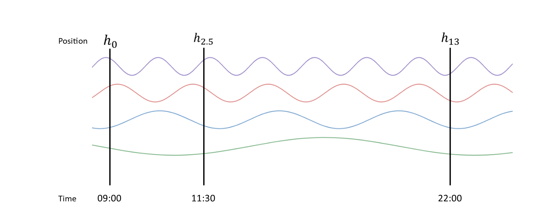
Figure 1: Sinusoidal functions discretization by time positions

$$\begin{aligned} TE_{(time,2i)}=sin(time/maxtime^{2i/d_{TE}})\end{aligned}$$ (3)

$$\begin{aligned} TE_{(time,2i+1)}=cos(time/maxtime^{2i/d_{TE}})\end{aligned}$$ (4)

To do it we redefine the equations based on irregular timestamps. Instead of a position indicator there is a $time$ variable, which is continuous. The dimension of TEs ($d_{TE}$) can parameterized and a $maxtime$ defines a maximum time that can be represented.

The relation between maximum time and TE dimension can be a limiting factor, as the maximum time increase the distance between TEs becomes smaller. To avoid this problem it is possible to increase TE dimensionality or set a reasonable maximum time.

The main pros of using TEs can be summarized as:

• Do not need any optimizable parameter, making it a model-free choice to deal with irregularity.

• Time delta can be linearly computed between two TEs, possibly improving long term dependencies recognition.

• All TEs have the same norm, avoiding big values as it is possible to happen with time delta descriptors when interval between observations are big.

4 Experiments

We evaluate the proposed algorithms on two benchmark tasks: in-hospital mortality and length of stay prediction. Booth tasks with the publicly available MIMIC-III dataset (Johnson et al., 2016). The following section we will briefly describe the data acquisition and prepossessing used, followed by the test results and discussion.

4.1 Dataset and training details

To assess the method performance we used the MIMIC-III benchmark dataset following the benchmark defined by Harutyunyan et al. (2017; 2019). With the available code we extracted sequences from in-hospital stays with first $48$ hours and split into training and testing set. This results in a dataset with $17,903$ training samples and $3,236$ test samples for in-hospital mortality after 48 hours task and $35,344/6,225$ for length of stay after 24 hours.

The dataset contains 18 variables with real values and five categorical. We did our own normalization of real variables to zero mean and unit variance, categorical variables are represented with one-hot encoding. At the length of stay task we also change labels from hours to days to avoid large outputs, to report results we change it back to hours.

To make the dataset even more irregular we removed randomly part of observed test data. By doing this we artificially create bigger time gaps to re-evaluate the models with an increased irregularity.

All models was trained with PyTorch (Paszke et al., 2017) on a P100, with batch size of 100 and AdamW (Loshchilov & Hutter, 2019) optimizer with amsgrad (Reddi et al., 2019). We performed a five fold cross-validation with 10 runs on each fold. The model with best validation performance (AUC for in-hospital mortality and Mean Absolute Error for length of stay) was selected to compose the average performance for test set. We report the mean and standard error of evaluation measures in test set.

4.2 Baselines and tests

To have a baseline we compared TEs primarily with binary masking with time interval indicators, as reported to have a good performance with RNNs in (Lipton et al., 2016). It was compared with the proposed method with a regular LSTM (Gers et al., 1999) and a Self-Attentive LSTM (Lin et al., 2017), as RNNs are reported to achieve best results with the evaluated tasks (Lipton et al., 2016, Shukla & Marlin, 2018, Bahadori & Lipton, 2019).

TEs was tested with dimension ($d_{TE}$) of 32 and maximum time of 48 hours. As binary masking dimension and concatenated TE increase input dimension we adjusted the LSTM hidden size to keep close the number of parameters of as describe at Table 1.

All neural models are connected to a 3 layers Multi-Layer Perceptron (MLP) with 32, 32, and 16 neurons. The last layers is a two neurons softmax for in-hospital mortality and one linear, with ReLU, for length of stay.

Table 1: Recurrent models compared and parameter count

Model	Alias	h	Nº of params
Vanilla LSTM	LSTM	34	15.5k
LSTM with Binary Masking	BM + LSTM	22	15.5k
LSTM with TE concatenated	catTE + LSTM	26	15.5k
Self-Attentive LSTM	SA-LSTM	32	15.5k
Self-Attentive LSTM with Binary Masking	BM SA-LSTM	22	15.5k
Self-Attentive LSTM with TE added	addTE + SA-LSTM	32	15.5k

The Self Attention was implemented as introduced in (Lin et al., 2017) with the only difference of using uni-directional LSTMs. The attention size ($d_{a}$) was 32 and the number of attentions ($r$) was 8. We also used the penalization term of $C=1^{-4}$

As the MIMIC III data are composed by multivariated series and we assume that Time Embeddings (TEs) should not be combined directly. So, we propose to use TEs in two different ways, as additional inputs, replacing missing mask, and as a latent space transformation, by adding TEs to the RNN output hidden state.

Figure 2: a) Additive model b) Concatenated model

To have also a baseline of non-recurrent models and assess the TE effect on them, we tested a four layer MLP and Linear/Logistic regression (linear for length of stay and logistic for in-hospital mortality task).

4.3 Results

Results for in-hospital mortality shows that self-attention seems to deteriorate the vanilla LSTM performance, but when added the TEs it got improved sufficiently to surpass it and achieve our better average result.

In the length of stay task TEs achieved better results, especially with bigger gaps at the reduced data test. TEs improved LSTM average error, but a slight worse explained variance, were binary masking had a better performance.

At Figure 3 and 4 we can see the performance of models when we randomly remove observed data from 100% to 10%. With length of stay task the LSTM with TE concatenated have a overall smaller absolute error than vanilla LSTM, being surpassed only by the binary mask. At in-hospital mortality we see a similar performance with TE SA-LSTM and LSTM with binary masking.

With non-recurrent models it is possible to observe how TEs does not rely on recurrence. It improved both linear/logistic regression and MLP.

Table 2: Results of Mean Absolute Error (MAE), Root Mean Squared Error (RMSE) and Explained Variance (EV) for length of stay task and Area Under ROC-Curve (AUC-ROC) and Average Precision (AP) for in-hospital mortality task. All results are in mean(standard deviation) format

Model	24h Length-of-Stay				48h In-hospital Mortality
	MAE	RMSE	EV		AUC-ROC	AP
Lin.R/Log.R	65.829(2.001)	133.178(2.777)	0.040(0.034)		0.783(0.003)	0.357(0.357)
BM + Lin.R/Log.R	68.343(2.453)	127.579(2.044)	0.104(0.029)		0.804(0.003)	0.369(0.369))
catTE + Lin.R/Log.R	69.585(0.870)	129.484(1.220)	0.077(0.017)		0.794(0.005)	0.359(0.359)
MLP	64.983(1.695)	137.949(14.440)	-0.053(0.236)		0.807(0.002)	0.374(0.374))
BM + MLP	63.181(3.120)	125.888(0.781)	0.133(0.007)		0.804(0.004)	0.365(0.365))
catTE + MLP	64.154(1.734)	129.259(2.115)	0.090(0.019)		0.805(0.003)	0.355(0.355))
LSTM	62.597(0.957)	122.284(0.266)	0.174(0.004)		0.855(0.002)	0.481(0.481)
BM + LSTM	61.666(0.702)	121.899(0.442)	0.180(0.006)		0.854(0.004)	0.485(0.485)
catTE + LSTM	62.354(0.686)	123.253(0.155)	0.164(0.002))		0.846(0.004)	0.476(0.476)
SA-LSTM	63.353(0.715)	122.976(0.215)	0.167(0.003)		0.851(0.005)	0.448(0.448)
BM + SA-LSTM	61.955(0.460)	121.667(0.089)	0.185(0.001)		0.854(0.006)	0.454(0.454))
addTE + SA-LSTM	62.591(0.321)	122.325(0.475)	0.173(0.006)		0.856(0.003)	0.482(0.482)

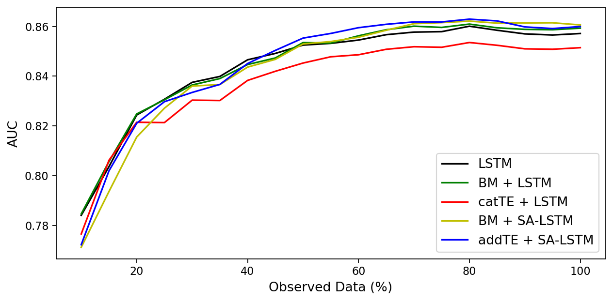
(a) AUC-ROC

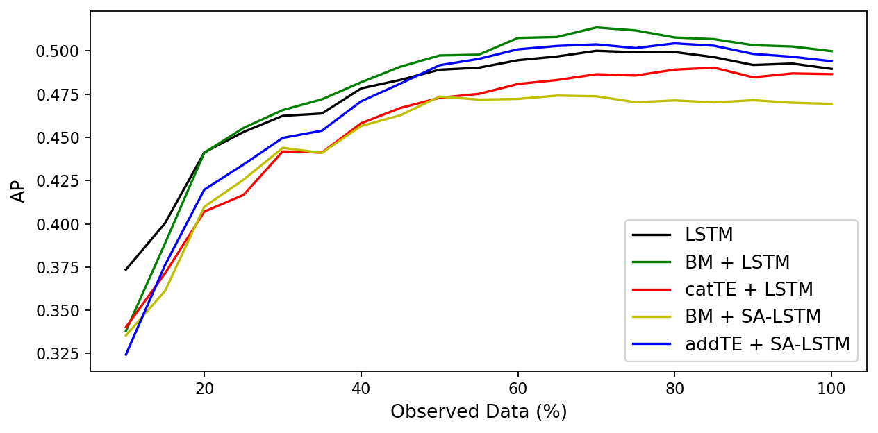
(b) Average Precision

Figure 3: Evaluation of models at in-hospital mortality with observed data from 10% to 100%

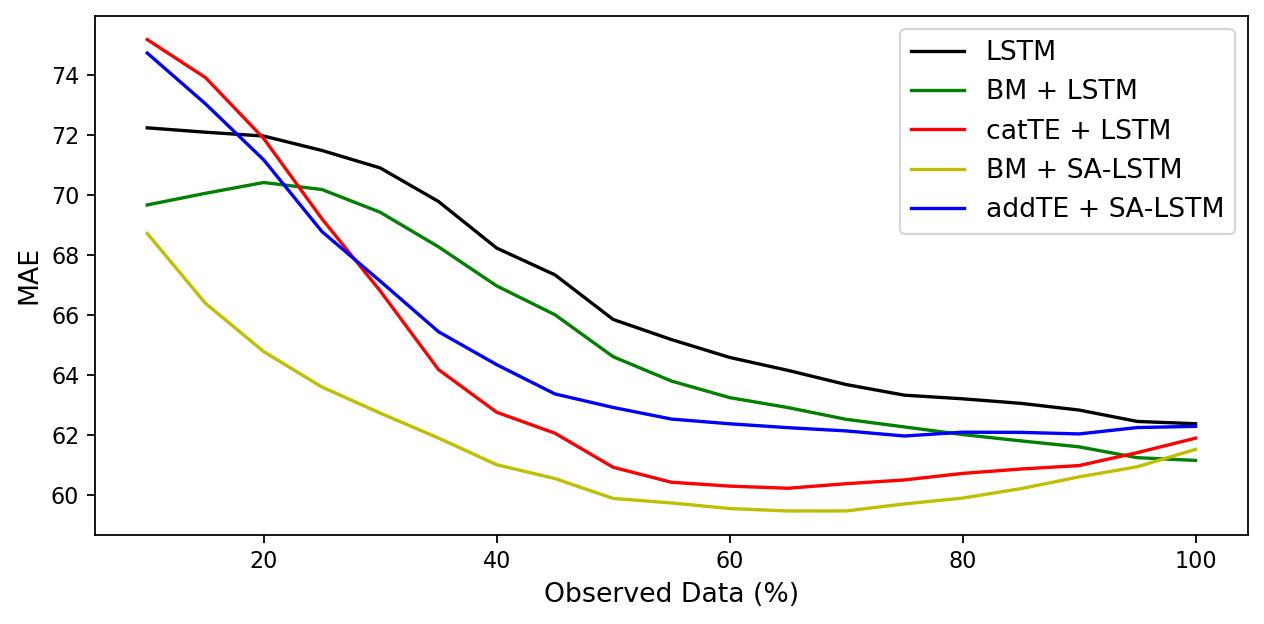
(a) Mean Absolute Error

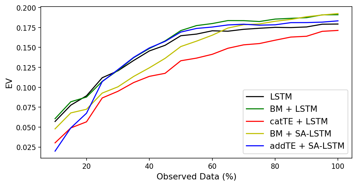
(b) Explained Variance

Figure 4: Evaluation of models at length of stay with observed data from 10% to 100%

5 Conclusions

This paper propose a novel method to represent hour time or dates as dense vectors to improve irregularly sampled time series. It was evaluated with two different approaches and evaluated in two tasks from the MIMIC III dataset. Our method showed some improvement with most models tested, including recurrent neural networks and classic machine learning methods.

Despite being outperformed by binary masking in some tests we believe TEs can still be an viable option. Specially to very irregular time series and high dimensional data, were TEs can be applied by addition without increasing the input dimensionality.

6 Future Work

We see a promising future for the method proposed. We expect to extend it to improve other types of irregular time-continuous data and also evaluate how can TE improve recent models proposed for irregularly time series, like the GRU-D (Che et al., 2018), interpolation networks (Shukla & Marlin, 2018) and Temporal-Clustering Regularization (Bahadori & Lipton, 2019). The code for TEs results reported will be publicly available in the future.

References

- Bahadori & Lipton (2019) Mohammad Taha Bahadori and Zachary Chase Lipton. Temporal-clustering invariance in irregular healthcare time series. arXiv preprint arXiv:1904.12206, 2019.
- (2) Seo-Jin Bang, Yuchuan Wang, and Yang Yang. Phased-lstm based predictive model for longitudinal ehr data with missing values.
- Che et al. (2018) Zhengping Che, Sanjay Purushotham, Kyunghyun Cho, David Sontag, and Yan Liu. Recurrent neural networks for multivariate time series with missing values. Scientific reports, 8(1):6085, 2018.
- Clark & Bjørnstad (2004) James S Clark and Ottar N Bjørnstad. Population time series: process variability, observation errors, missing values, lags, and hidden states. Ecology, 85(11):3140–3150, 2004.
- Gehring et al. (2017) Jonas Gehring, Michael Auli, David Grangier, Denis Yarats, and Yann N. Dauphin. Convolutional sequence to sequence learning. CoRR, abs/1705.03122, 2017. URL http://arxiv.org/abs/1705.03122.
- Gers et al. (1999) Felix A Gers, Jürgen Schmidhuber, and Fred Cummins. Learning to forget: Continual prediction with lstm. 1999.
- Harutyunyan et al. (2017) Hrayr Harutyunyan, Hrant Khachatrian, David C Kale, Greg Ver Steeg, and Aram Galstyan. Multitask learning and benchmarking with clinical time series data. arXiv preprint arXiv:1703.07771, 2017.
- Harutyunyan et al. (2019) Hrayr Harutyunyan, Hrant Khachatrian, David C Kale, Greg Ver Steeg, and Aram Galstyan. Multitask learning and benchmarking with clinical time series data. Scientific data, 6(1):96, 2019.
- Johnson et al. (2016) Alistair EW Johnson, Tom J Pollard, Lu Shen, H Lehman Li-wei, Mengling Feng, Mohammad Ghassemi, Benjamin Moody, Peter Szolovits, Leo Anthony Celi, and Roger G Mark. Mimic-iii, a freely accessible critical care database. Scientific data, 3:160035, 2016.
- Lin et al. (2017) Zhouhan Lin, Minwei Feng, Cicero Nogueira dos Santos, Mo Yu, Bing Xiang, Bowen Zhou, and Yoshua Bengio. A structured self-attentive sentence embedding. arXiv preprint arXiv:1703.03130, 2017.
- Lipton et al. (2016) Zachary C Lipton, David C Kale, and Randall Wetzel. Modeling missing data in clinical time series with rnns. arXiv preprint arXiv:1606.04130, 2016.
- Little & Rubin (2019) Roderick JA Little and Donald B Rubin. Statistical analysis with missing data, volume 793. John Wiley & Sons, 2019.
- Loshchilov & Hutter (2019) Ilya Loshchilov and Frank Hutter. Decoupled weight decay regularization. In International Conference on Learning Representations, 2019. URL https://openreview.net/forum?id=Bkg6RiCqY7.
- Marlin et al. (2012) Benjamin M Marlin, David C Kale, Robinder G Khemani, and Randall C Wetzel. Unsupervised pattern discovery in electronic health care data using probabilistic clustering models. In Proceedings of the 2nd ACM SIGHIT international health informatics symposium, pp. 389–398. ACM, 2012.
- Paszke et al. (2017) Adam Paszke, Sam Gross, Soumith Chintala, Gregory Chanan, Edward Yang, Zachary DeVito, Zeming Lin, Alban Desmaison, Luca Antiga, and Adam Lerer. Automatic differentiation in pytorch. In NIPS-W, 2017.
- Reddi et al. (2019) Sashank J Reddi, Satyen Kale, and Sanjiv Kumar. On the convergence of adam and beyond. arXiv preprint arXiv:1904.09237, 2019.
- Scargle (1982) Jeffrey D Scargle. Studies in astronomical time series analysis. ii-statistical aspects of spectral analysis of unevenly spaced data. The Astrophysical Journal, 263:835–853, 1982.
- Schulz & Stattegger (1997) Michael Schulz and Karl Stattegger. Spectrum: Spectral analysis of unevenly spaced paleoclimatic time series. Computers & Geosciences, 23(9):929–945, 1997.
- Shukla & Marlin (2018) Satya Narayan Shukla and Benjamin Marlin. Interpolation-prediction networks for irregularly sampled time series. 2018.
- Vaswani et al. (2017) Ashish Vaswani, Noam Shazeer, Niki Parmar, Jakob Uszkoreit, Llion Jones, Aidan N. Gomez, Lukasz Kaiser, and Illia Polosukhin. Attention is all you need. CoRR, abs/1706.03762, 2017. URL http://arxiv.org/abs/1706.03762.
- Yadav et al. (2018) Pranjul Yadav, Michael Steinbach, Vipin Kumar, and Gyorgy Simon. Mining electronic health records (ehrs): a survey. ACM Computing Surveys (CSUR), 50(6):85, 2018.
- Zhang et al. (2018) Jinghe Zhang, Kamran Kowsari, James H Harrison, Jennifer M Lobo, and Laura E Barnes. Patient2vec: A personalized interpretable deep representation of the longitudinal electronic health record. IEEE Access, 6:65333–65346, 2018.