BetheSF: Efficient computation of the exact tagged-particle propagator in single-file systems via the Bethe eigenspectrum

Abstract

Single-file diffusion is a paradigm for strongly correlated classical stochastic many-body dynamics and has widespread applications in soft condensed matter and biophysics. However, exact results for single-file systems are sparse and limited to the simplest scenarios. We present an algorithm for computing the non-Markovian time-dependent conditional probability density function of a tagged-particle in a single-file of $N$ particles diffusing in a confining external potential. The algorithm implements an eigenexpansion of the full interacting many-body problem obtained by means of the coordinate Bethe ansatz. While formally exact, the Bethe eigenspectrum involves the generation and evaluation of permutations, which becomes unfeasible for single-files with an increasing number of particles $N$. Here we exploit the underlying exchange symmetries between the particles to the left and to the right of the tagged-particle and show that it is possible to reduce the complexity of the algorithm from the worst case scenario $\mathcal{O}(N!)$ down to $\mathcal{O}(N)$. A C++ code to calculate the non-Markovian probability density function using this algorithm is provided. Solutions for simple model potentials are readily implemented incl. single-file diffusion in a flat and a ’tilted’ box, as well as in a parabolic potential. Notably, the program allows for implementations of solutions in arbitrary external potentials under the condition that the user can supply solutions to the respective single-particle eigenspectra.

PROGRAM SUMMARY

Program Title: BetheSF
Licensing provisions: MIT
Programming language: C++ (C++17 support required)
Supplementary material: makefile, README, SingleFileBluePrint.hpp
Nature of problem:
Diffusive single-files are mathematical models of effectively one-dimensional strongly correlated many-body systems. While the dynamics of the full system is Markovian, the diffusion of a tracer-particle in a single-file is an example of non-Markovian and anomalous diffusion. The many-body Fokker-Planck equation governing the system’s dynamics can be solved using the coordinate Bethe ansatz. A naïve implementation of such a solution runs in non-polynomial time since it requires the generation of permutations of the elements of a multiset.
Solution method:
In this paper we show how, exploiting the exchange symmetries of the system, it is possible to reduce the complexity of the algorithm to evaluate the solution, using a permutation-generation algorithm, from $\mathcal{O}(N!)$ in the worst case scenario to $\mathcal{O}(N)$ in the best case scenario, which corresponds to tagging the first or the last particle, where $N$ stands for the number of particles in the single-file.
Additional comments including Restrictions and Unusual features: The code may overflow for large single-files $N\geq 170$. All the benchmarks ran on the following CPU: Intel Xeon E3-1270 v2 3.50 GHz 4 cores. The compiler used is g++ 7.3.1 (SUSE Linux) with the optimization -O3 turned on. The code to produce all the data in the figures is included in the files: figure1.cpp, figure2.cpp, figure3.cpp, figure4a.cpp and figure4b.cpp.

1 Introduction

Single-file diffusion refers to the dynamics of one-dimensional systems composed of identical hard-core particles, that is, to many-particle diffusion subject to non-crossing boundary conditions. Diffusive single-file models are a paradigm for the stochastic dynamics of classical strongly correlated many-body systems. As such they have been studied extensively both theoretically (see e.g. [1, 2, 3, 4, 5, 6, 7, 8, 9, 10]) as well as experimentally ([11, 12, 13]). Single-file diffusion underlies the dynamics in biological channels [14], molecular search processes of transcription factors in gene regulation [15], transport in zeolites [16, 17] and superionic conductors [18], and diverse phenomena in soft matter systems [19].

Whereas the dynamics of the entire $N$-particle single-file is Markovian, the typically observed “tagged-particle” diffusion – the projection of the many-body dynamics onto the motion of a single tracer particle – is strongly non-Markovian [10]. Namely, by focusing on a tagged-particle alone, the $N-1$ remaining so-called latent degrees of freedom (i.e. the coordinates of the remaining particles) that become coarse-grained out, relax on exactly the same time scale as the tagged particle [10]. This renders single-file diffusion somewhat special as compared to other physical examples probing low-dimensional projections, such as for example the dynamics of individual protein molecules [20] involving degrees freedom with relaxation times that span several orders of magnitude in time [21]. As there are no “fast” degrees of freedom in a single-file, low-dimensional projections give rise to strong memory effects, i.e. the Markov property is said to be strongly broken. In other words, the dynamics of a tagged-particle is fundamentally different (by extent as well as duration) from the adiabatic, Markovian approximation of the dynamics of a single particle diffusing in a potential of mean force created if the remaining particles were to relax to equilibrium instantaneously [10].

Tagged-particle diffusion in a single-file is also a representative toy model for diffusion in so-called crowded systems, in particular when the dynamics is effectively one-dimensional and anomalous [22], i.e. when the mean squared displacement of a particle $\langle(x(t)-x(0))^{2}\rangle\propto t^{\alpha}$ (where $\langle\cdot\rangle$ denotes the average over an ensemble of trajectories) is not linear in time as in the case of (normal) Brownian motion (i.e. $\alpha_{\rm Brown}=1$) but scales sub-linearly with $\alpha=1/2$, which is referred to as subdiffusion [23]. The theoretical analysis of tagged-particle dynamics has been carried out by several different techniques: the so-called “reflection principle“ applicable to single-files with both finite and infinite number of elements [4], Jepsen mapping for the central particle in a finite [5] or infinite single-file [24], the so-called momentum Bethe ansatz for a finite single-file [7], harmonization techniques for infinite single-files [8], etc.

Here, we focus on the propagator (or the ”non-Markovian Green’s function“) of a tagged-particle in a finite single-file of $N$ particles diffusing in an arbitrary confining potential, that is, the conditional probability density function to find the tagged-particle at position $x$ at a time $\tau$ assuming that at $\tau=0$ it was at $x_{0}$, while the positions of the remaining $N-1$ particles were drawn from the equilibrium distribution compatible with the initial position of the tagged-particle. In the past few years a number of detailed analyses of ensemble- [7, 10] and time- [9, 10] averaged physical observables have been carried out focusing on the motion of a tagged-particle in a single-file, which provided a generic, conceptual insight into the emergence of memory in projection-induced non-Markovian dynamics.

In our previous work [9, 10] we determined the propagator exactly by means of the coordinate Bethe ansatz (CBA) [25]. The power of the CBA lies in the fact that it diagonalizes the many-body Fokker-Planck operator that governs the dynamics of the single-file. In other words, it expresses the dynamics of the full $N$-body system in a given potential in terms of a complete set of eigenfunctions and corresponding eigenvalues, which describe exactly how the system relaxes to equilibrium in terms of irreducible collective relaxation modes on different time-scales. By projecting these collective modes onto the motion of a tagged-particle we were able to disentangle the microscopic, collective origin of subdiffusion and memory in tagged-particle dynamics in simple confining potentials [9, 10, 26].

However, the implementation of the analytical results obtained by the CBA poses a computational challenge since it involves an algorithm whose complexity is non-polynomial in $N$. Here we present an efficient algorithm (that in some cases runs in polynomial time) for evaluating the tagged-particle propagator that exploits the exchange-symmetry of the problem. We also present a C++ code to perform such a computation for selected examples. The code is easily extendable to other potentials.

Notably, a common alternative method to analyze tagged-particle dynamics in finite single-files is to perform Brownian Dynamics computer simulations. To do so efficient algorithms have been designed based on the Gillespie algorithm[6], on the Ermak algorithm [27] or on the Verlet algorithm [28]. Nevertheless, these algorithms may still suffer from time- and space- discretization artifacts since they only provide an approximate solution to the problem. Moreover, they do not readily reveal the collective relaxation eigenmodes, nor do they establish how these affect tagged-particle motion. In addition, the computational cost of such Brownian Dynamics simulations is much larger than the one of the present algorithm (for a comparison see Section 5).

2 Problem and solution by means of the coordinate Bethe ansatz

The evolution of the (Markovian) probability density function of a diffusive single-file of $N$ particles in the over-damped regime under the influence of an external force $F(x)=-\partial_{x}U(x)$, $G(\mathbf{x},\tau|\mathbf{x}_{0})$, evolving from an initial condition $G(\mathbf{x},0|\mathbf{x}_{0})=\delta(\mathbf{x}-\mathbf{x}_{0})$ is described by the Fokker-Planck equation

$$\left[\partial_{\tau}-\sum_{i=1}^{N}\left(D\partial_{x_{i}}^{2}-\mu\partial_{x_{i}}F(x_{i})\right)\right]G(\mathbf{x},\tau|\mathbf{x}_{0}) = 0,$$

$$\left(\partial_{x_{i+1}}-\partial_{x_{i}}\right)G(\mathbf{x},\tau,\mathbf{x}_{0})\left|{}_{x_{i+1}=x_{i}}\right. = 0,\quad\forall i,$$ (1)

where $D$ is the diffusion coefficient, $\mu=D/k_{\mathrm{B}}T$ is the mobility given by the fluctuation-dissipation theorem, and $\delta(\mathbf{x}-\mathbf{x}_{0})=\prod_{i=1}^{N}\delta(x_{i}-x_{0i})$. Eq. (1) is accompanied by appropriate external boundary conditions for the first and last particle of the single-file. Here we will only consider so-called natural (’zero probability at infinity’, i.e. $\lim_{|\mathbf{x}|\to\infty}G(\mathbf{x},\tau|\mathbf{x}_{0})=0$) or reflecting (’zero flux’) boundary conditions, which are selected according to the specific nature of the external potential $U(x)$. We will assume that $U(x)$ is sufficiently confining to assure that the eigenspectrum of the generator $\hat{L}_{N}\equiv\sum_{i=1}^{N}[D\partial_{x_{i}}^{2}-\mu\partial_{x_{i}}F(x_{i})]$ is discrete [29]. In Eq. (1) we assumed that each particle experiences the same external force $F(x)$ and throughout we will assume that $D$ is equal for all particles. Note that the corresponding over-damped (Itô) Langevin equation that describes individual trajectories of the single-file and would be integrated numerically in a Brownian Dynamics simulation reads

$$dx_{i}(t)=\mu F(x_{i}(t))dt+\sqrt{2D}dW^{i}_{t},\,\langle dW_{t}\rangle=0,\,\langle dW^{i}_{t}dW^{j}_{t^{\prime}}\rangle=\delta_{ij}\delta(t-t^{\prime})dt,\forall i,$$ (2)

where $dW_{t}$ is an increment of the Wiener process (Gaussian white noise), whereby we must enforce that particles remain ordered at all times, i.e. $x_{i}(t)\leq x_{i+1}(t),\forall i,t$.

The boundary value problem in Eq. (1) can be solved exactly by means of the coordinate Bethe ansatz [25], which requires that we (only) know the eigenexpansion of the single-particle Green’s function. That is, we are required to solve the following single-particle Fokker-Planck equation with the same external boundary conditions

$$(\partial_{\tau}-\hat{L}_{1})\Gamma(x_{i},\tau|x_{0i})=0$$ (3)

with initial condition $\Gamma(x_{i},0|x_{0i})=\delta(x_{i}-x_{0i})$, which can be conveniently expressed by means of a (bi)spectral expansion

$$\Gamma(x_{i},\tau|x_{0i})=\sum_{k=0}^{\infty}\psi_{k_{i}}^{R}(x_{i})\psi_{k_{i}}^{L}(x_{0i})\mathrm{e}^{-\lambda_{k_{i}}\tau},$$ (4)

where $-\lambda_{k_{i}}<0,\forall i>0$ and $\lambda_{0}=0$ are the eigenvalues, and $\psi_{k_{i}}^{L/R}(x)$ are respectively the $k_{i}$th left and the right eigenfunction of the operator $\hat{L}_{1}$, which form a complete bi-orthonormal basis. Here we assume detailed balance to be obeyed and hence $\psi_{l}^{R}(x)\propto\mathrm{e}^{-\beta U(x)}\psi_{l}^{L}(x)$ [30], where $\beta=1/(k_{B}T)$ is the inverse of the thermal energy. The solution to the many-body Fokker-Planck equation can be written as

$$G(\mathbf{x},\tau|\mathbf{x}_{0})=\sum_{\mathbf{k}}\Psi_{\mathbf{k}}^{R}(\mathbf{x})\Psi_{\mathbf{k}}^{L}(\mathbf{x}_{0})\mathrm{e}^{-\Lambda_{\mathbf{k}}\tau}.$$ (5)

The many-body eigenvalue $\mathbf{k}$ corresponds to a multiset containing the $N$ natural numbers $\{k_{1},k_{2},\cdots,k_{N}\}$ and $\mathbf{0}$ denotes the unique ground state of the many-body system in which each single-particle eigenvalue is equal to zero. Each pair of many-body eigenvalues and eigenfunctions satisfies the eigenvalue problem

$$\hat{L}_{N}\Psi_{\mathbf{k}}^{R}=\Lambda_{\mathbf{k}}\Psi_{\mathbf{k}}^{R}.$$ (6)

The Bethe ansatz solution postulates that the right eigenfunction has the following form

$$\Psi_{\mathbf{k}}^{R}=\hat{O}_{\mathbf{x}}\sum_{\{\mathbf{k}\}}\prod_{i=1}^{N}c_{i}\psi_{k_{i}}^{R}(x_{i});$$ (7)

where $\sum_{\{\mathbf{k}\}}$ denotes the sum over all the possible permutations of the multiset $\mathbf{k}$ (see A) and $\hat{O}_{\mathbf{x}}$ denotes the particle-ordering operator defined as

$$\hat{O}_{\mathbf{x}}\equiv\prod_{i=2}^{N}\Theta(x_{i}-x_{i-1}),$$ (8)

where $\Theta(x)$ denotes the Heaviside step function.

The $N$ constants $\{c_{i}\}$ and the many-body eigenvalue are fixed imposing the $N-1$ internal boundary conditions in Eq. (1) alongside the pair of external boundary conditions. This leads to the many-body eigenvalue

$$\Lambda_{\mathbf{k}}=\sum_{i=1}^{N}\lambda_{k_{i}},$$ (9)

and in the case of zero-flux boundary conditions all $c_{i}$ turn out to be equal to one. Finally, a proper orthonormalization between left and right many-body eigenfunctions must be assured, for example

$$\Psi_{\mathbf{k}}^{L/R}(\mathbf{x})=\mathcal{N}^{-1/2}\hat{O}_{\mathbf{x}}\sum_{\{\mathbf{k}\}}\prod_{i=1}^{N}\psi_{k_{i}}^{L/R}(x_{i}),$$ (10)

where the normalization factor $\mathcal{N}$ is equal to the number of permutations of the multiset $\mathbf{k}$ (see A).

Here we are interested in the non-Markovian Green’s function referring to the propagation of a tagged-particle starting from a fixed initial condition $x_{0i}$ while the remaining particles are drawn from those equilibrium configurations that are compatible with the initial condition of the tagged-particle [10]

$$\mathcal{G}(x_{i},\tau|x_{0i})=V_{\mathbf{0}\mathbf{0}}^{-1}(x_{0i})\sum_{\mathbf{k}}V_{\mathbf{0}\mathbf{k}}(x_{i})V_{\mathbf{k}\mathbf{0}}(x_{0i})\mathrm{e}^{-\Lambda_{\mathbf{k}}\tau},$$ (11)

where the ’overlap elements’ are defined as

$$V_{\mathbf{k}\mathbf{l}}(z)=\int d\mathbf{x}\delta(z-x_{i})\Psi_{\mathbf{k}}^{L}(\mathbf{x})\Psi_{\mathbf{l}}^{R}(\mathbf{x}),$$ (12)

and $\delta(x)$ is Dirac’s delta. In the specific case of equilibrated initial conditions for background particles only the special cases

$$V_{\mathbf{k}\mathbf{0}}(z) = \int d\mathbf{x}\delta(z-x_{i})\Psi_{\mathbf{k}}^{L}(\mathbf{x})\Psi_{\mathbf{0}}^{R}(\mathbf{x}),$$

$$V_{\mathbf{0}\mathbf{k}}(z) = \int d\mathbf{x}\delta(z-x_{i})\Psi_{\mathbf{0}}^{L}(\mathbf{x})\Psi_{\mathbf{k}}^{R}(\mathbf{x})$$ (13)

are important. Note that any numerical implementation of Eq. (11) involves a truncation at some maximal eigenvalue $\Lambda_{\mathbf{M}}$. The ordering operator allows us to evaluate the integrals (13) as nested integrals, i.e.

$$\mathop{\mathrlap{\int}{\,}n}_{a}^{b}f(\mathbf{x})d\mathbf{x}=\int_{a}^{b}dx_{1}\int_{x_{1}}^{b}dx_{2}\cdots\int_{x_{N-2}}^{b}dx_{N-1}\int_{x_{N-1}}^{b}dx_{N}f(\mathbf{x}).$$ (14)

Since by construction the integrand is invariant under exchange of the $\{x_{i}\}$ coordinates we can take advantage of the so-called extended phase-space integration [31] and greatly simplify the multi-dimensional nested integral to a product of one-dimensional integrals

$$\mathop{\mathrlap{\int}{\,}n}_{a}^{b}f(\mathbf{x})\delta(z-x_{i})d\mathbf{x}=\left(\prod_{j=1}^{i-1}\int_{a}^{z}dx_{j}\right)\left(\prod_{j=i+1}^{N}\int_{z}^{b}dx_{j}\right)\frac{f(x_{i}=z,\{x_{j},j\neq i\})}{N_{L}!N_{R}!},$$ (15)

where $a$ and $b$ are the lower and upper boundary of the domain, respectively, and $N_{L}$($N_{R}$) is the number of particles to the left(right) of the tagged one. These last two equations allow us the write Eq. (12) as

$$V_{\mathbf{k}\mathbf{l}}(z)=\frac{m_{\mathbf{l}}}{N_{L}!N_{R}!}\sum_{\{\mathbf{k}\}}\sum_{\{\mathbf{l}\}}T_{i}(z)\prod_{j=1}^{i-1}L_{j}(z)\prod_{j=i+1}^{N}R_{j}(z),$$ (16)

where $m_{\mathbf{l}}$ is the multiplicity of the multiset $\mathbf{l}$ defined in A and we have introduced the auxiliary functions

$$T_{i}(z)=\psi^{L}_{k_{i}}(z)\psi^{R}_{l_{i}}(z),$$ (17a)

$$L_{j}(z)=\int_{a}^{z}dx\psi^{L}_{k_{j}}(x)\psi^{R}_{l_{j}}(x),$$ (17b)

$$R_{j}(z)=\int_{z}^{b}dx\psi^{L}_{k_{j}}(x)\psi^{R}_{l_{j}}(x).$$ (17c)

Once substituted into Eq. (11) Eqs. (16-17c) deliver the tagged particle propagator sought for.

3 Avoiding permutations

Algorithm 1 Calculate $V_{\mathbf{k}\mathbf{l}}(z)$

1:.

• $\mathbf{k},\mathbf{l}$ multisets;

• $z\in\mathbb{R},a\leq z\leq b$;

• functions: $T_{i}(z),L_{j}(z),R_{j}(z)$;

• a function to generate all the permutation of multiset $P(\mathbf{k})$;

• a function to calculate the number of permutation of a multiset: $\mathcal{N}_{\mathbf{k}}$;

• a function to generate all the $t$-combinations of a multiset $C(\mathbf{k},t)$;

• a function to compute the multiset difference $\mathbf{k}\setminus\mathbf{l}$;

• a function to create the largest set from a multiset $\tilde{k}=S(\mathbf{k})$;

2:calculate $\mathcal{N}_{\mathbf{k}}$ and $\mathcal{N}_{\mathbf{l}}$ and pick the multiset with the smallest number of permutations (let us assume it is $\mathbf{l}$);

3:initialize $s\leftarrow 0$;

4:for all $\mathbf{l}^{*}\in P(\mathbf{l})$ do

5:     create the multiset of pairs $\mathbf{p}=\{\{k_{1},l^{*}_{1}\},\cdots,\{k_{N},l^{*}_{N}\}\}$;

6:     $\tilde{u}\leftarrow S(\mathbf{p})$;

7:     for $u\in\tilde{u}$ do

8:         $\mathbf{r}\leftarrow\mathbf{p}\setminus u$;

9:         $t\leftarrow\mathrm{min}(N_{L},N_{R})$;

10:         initialize $s_{1}\leftarrow 0$;

11:         for all $\mathbf{s}\in C(\mathbf{r},t)$ do

12:              $\mathbf{d}\leftarrow\mathbf{r}\setminus\mathbf{s}$

13:              if $t=N_{L}$ then

14:                  $a\leftarrow T_{i}(z)\prod_{j\in\mathbf{s}}L_{j}(z)\prod_{j\in\mathbf{d}}R_{j}(z)$;

15:              else

16:                  $a\leftarrow T_{i}(z)\prod_{j\in\mathbf{d}}L_{j}(z)\prod_{j\in\mathbf{s}}R_{j}(z)$

17:              end if

18:              $s_{1}+=\mathcal{N}_{\mathbf{s}}\mathcal{N}_{\mathbf{d}}a$;

19:         end for

20:         $s+=s_{1}$;

21:     end for

22:end for

23:return $\frac{m_{\mathbf{l}}}{N_{L}!N_{R}!}s$.

Although the extended phase-space integration (cf Eqs. (12) and  (16)) substantially simplifies the integrals involved in the computation of the tagged particle propagator we still need to sum over all the permutations of $\mathbf{l}$ and $\mathbf{k}$ in Eq. (16). A brute force (or naïve) approach is thus not feasible, not even for rather small single-files since we need to evaluate the products $V_{\mathbf{0}\mathbf{k}}(x_{i})V_{\mathbf{k}\mathbf{0}}(x_{0i})$ in Eq. (11) up to $2\times N!$ times in the worst case scenario for a calculation involving only the Green’s function; and for a general element $V_{\mathbf{l}\mathbf{k}}$ up to $(N!)^{2}$.

The main contribution of this paper is Algorithm 1 that reduces the number of terms in the Bethe ansatz solution entering Eq. (16) that need to be computed explicitly. Namely, since the full single-file diffusion model is symmetric with respect to the exchange of particles many terms arising from the permutations of the eigennumbers of the multisets in Eq. (16) happen to be identical. Algorithm 1 counts how many terms are equal and computes only those that are unique, and does so only once. These unique terms are then multiplied by their respective multiplicity and summed up to yield the result Eq. (11). Algorithm 1 thereby avoids going through the large number of equivalent permutations of the multisets in the sum with the larger number of terms between $\sum_{\{\mathbf{k}\}}$ and $\sum_{\{\mathbf{l}\}}$ in Eq. (16). In the specific case of the tagged-particle Green’s function defined in Eq. (11), where one of the two multisets $\{\mathbf{k}\},\{\mathbf{l}\}$ corresponds to the ground state (having only one permutation), the algorithm in fact avoids permutations entirely.

More precisely (i.e. for a general $V_{\mathbf{k}\mathbf{l}}(x_{i})$), the algorithm first generates all permutations of the multiset having the smallest number of permutations $P(\mathbf{l})$ (for sake of simplicity let us assume that this is the multiset $\mathbf{l}$ with $\mathcal{N}_{\mathbf{l}}$ distinct permutations). Then, for each of these permutations a multiset of pairs is created: $\mathbf{p}=\{\{k_{1},l^{*}_{1}\},\cdots,\{k_{N},l^{*}_{N}\}\}$. The function $S(\mathbf{p})$ selects the largest possible set from $\mathbf{p}$ and generates for each element $u$ of the resulting set the ’difference multiset’: $\mathbf{r}=\mathbf{p}\setminus u$. In the following it determines $t=\mathrm{min}(N_{L},N_{R})$ and all the $t-$combinations of $\mathbf{r}$ are generated via $C(\mathbf{r},t)$ (note that $t$ here does not refer to time). For each of these combinations $\mathbf{s}$ the complementary multiset $\mathbf{d}=\mathbf{r}\setminus\mathbf{s}$ is created and the number of permutations of $\mathbf{s}$ and $\mathbf{d}$ is computed. Finally, the products in Eq. (16) are calculated (where $u$ is the pair of eigennumbers belonging to the tagged-particle) and accounted for their multiplicity.

In summary, our algorithm exploits the fact that the extended phase-space integration allows us to ignore the ordering of the particles to the left and to the right of the tagged-particle, respectively. A consequence of this symmetry is that several terms that appear in Eq. (16) are identical. Therefore, we can substitute the permutations of one multiset in Eq. (16) with all its combinations that are not tied to any ordering by definition. This makes the algorithm more efficient. A pseudocode-implementation is presented in Algorithm 1 and an explicit flowchart is depicted in Fig. 1. The reduction of the computational time achieved by our algorithm compared to a naïve implementation is presented in Fig. 2.

Figure 1: The flowchart of Algorithm 1. The steps #13 and #15 are not reported for spatial constraints and can be found in the explanation of the algorithm.

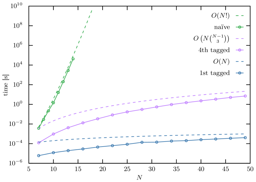
Figure 2: Computational time (in seconds) required to calculate $V_{\mathbf{k}\mathbf{0}}$ for a single-file confined to a flat box depending on the number of particles in the single-file $N$; the $\mathbf{k}$-multiset has been chosen to represent the worst case scenario, i.e. $\mathbf{k}=\{1,2,\cdots,N\}$. The green line corresponds to the running time of the naïve implementation for comparison (which does not depend on which particle is tagged), while the blue and purple lines depict the running time of our program tagging the first and fourth particle, respectively. Dashed lines depict the computational complexity for the various cases.

Computational complexity of Algorithm 1

The computational complexity of the algorithm can be derived by following its flow (see Fig. 1). For the sake of simplicity we will (only initially) assume that the multiset $\mathbf{l}$ has only one possible permutation. Let $\mathcal{U}$ be the number of unique elements belonging to the multiset $\mathbf{k}$. Then for each unique element $u\in\mathbf{k}$ we need to iterate over all the $t$-combinations of the multiset $\mathbf{k}\setminus u$, where $t=\mathrm{min}(N_{L},N_{R})$. The number of these combinations is given by the function $\mathcal{M}(N-1,t)$ – an algorithm describing and computing this function is presented in A. Hence, the complexity of the algorithm is given by $\mathcal{O}(\mathcal{U}\cdot\mathcal{M}(N-1,\mathrm{min}(N_{L},N_{R}))$. In the worst-case scenario, in which all the elements of $\mathbf{k}$ are different, the complexity is $\mathcal{O}\left(N\cdot\binom{N-1}{\mathrm{min}(N_{L},N_{R})}\right)$. However, even in this worst case scenario the algorithm scales linearly $\mathcal{O}(N)$ in the number of particles if we tag the first or the last particle (see Fig. 2). In the general case when $\mathbf{l}\neq\mathbf{0}$, i.e. the one in which $\mathbf{l}$ admits more permutations (which, however, is not required for evaluating Eq. (11)), the complexity deteriorates fast since the evaluation of all permutations of $\mathbf{l}$ must be considered; the computational complexity in this case is $\mathcal{O}(\mathcal{N}_{\mathbf{l}}\cdot\mathcal{U}\cdot\mathcal{M}(N-1,\mathrm{min}(N_{L},N_{R}))$, where $\mathcal{N}_{\mathbf{l}}$ is the number of permutations with repetitions of $\mathbf{l}$ and we assume that $\mathcal{N}_{\mathbf{l}}\leq\mathcal{N}_{\mathbf{k}}$.

4 Implementation

The main goal of the code attached to this article is to compute the Green’s function of any tagged-particle in a single-file of $N$ elements given a potential $U(x)$. For this reason we opt for an object-oriented approach that allows the user to easily extend the code to incorporate any potential satisfying the constraints on $\hat{L}_{N}$. The code defines the abstract base class: classSingleFile (in SingleFile.hpp) responsible for the interface and for the functions that are responsible for the computation of the overlap elements (Eq. (16)). Conversely, all functions directly related to some specific potential $U(x)$ are private pure abstract base functions and must be implemented by the user in a derived class.

In our codebase we provide three different derived classes:
class SingleFileFlat : public SingleFile;,
class SingleFileOnSlope : public SingleFile;,
class SingleFileHarmonic : public SingleFile; in the header file SingleFileDerived.hpp, covering several different ’canonical’ cases of single-file systems.

The base class

The base class class SingleFile provides a common interface to all single-file systems. It contains the following functions: the equilibrium probability density function virtual double eq_prob(constdouble x) const;,
the two-point joint density
double joint2dens(const double x, const double t, const doublex0);
and the Green’s function
double green_function(const double x, const double t, const doublex0);
for a specific tagged-particle implementing the analytical solution in Eq. (11). The function evaluating the equilibrium probability density function of a tagged-particle, i.e. $\mathcal{G}_{\mathrm{eq}}(x_{i})=\lim_{t\to\infty}\mathcal{G}(x_{i},\tau|x_{0i})$, is virtual since for a given potential $U(x)$ it often has a relatively simple form. In addition, naïve implementations directly computing all permutations have also been defined in the interface: double joint2dens_naive(const double x, const double t, const double x0);
and double green_function_naive(const double x, const double t, const double x0);.
These two functions call the function
double Vkl_element_naive(std::vector<int>& k_vec, std::vector<int>& l_vec, const double x) const;
that implements slavishly Eq. (12). Finally, the interface of the class is completed by several tiny functions that allow changing the parameters of an instance of the class, like the tagged-particle or the diffusion coefficient $D$.

The base class is also responsible for the internal machinery to use our fast algorithm implementing (among its private members):
doubleVkl_element(std::vector<int>& k_vec, std::vector<int>& l_vec, constdouble x) const;;
and its specialized versions, defined by default in its terms:
virtual double V0k_element(std::vector<int>& k_vec, const double x)const; and
virtual double Vk0_element(std::vector<int>& k_vec, const double x)const;.

These specialized versions are made virtual to allow a derived class to override them if they require special settings (one such example is the single-file in a linear potential). The declarations and definitions of these functions can be found in the files SingleFile.hpp and SingleFile.cpp. Our algorithm computes the $t$-combinations of a multiset and this feature is provided by the friend class template<typename T>class UCombinations; that implements (in the file combinations.hpp) a classical algorithm given in [32]. We use std::next_permutation for the computation of permutations. Finally, this base abstract class defines the private members responsible for the calculation of the single-particle eigenvalues and for the evaluation of Eqs. (17c). These are pure virtual functions since they depend on the specific external potential, and hence they must be implemented by the derived class. Finally, the pure virtual function virtual int eigenfunction_condition(const int i)const=0;
defines the rule to initialize the private member
std::vector<std::vector<int>>eigenfunction_store; that contains (row-wise) all the multisets considered in the evaluation of Eq. (5) for a given specific potential $U(x)$. For this reason the derived class is responsible for initializing this last member (in its constructor, for example). We provide the protected function void eigenfunction_store_init(); to initialize this data structure (details are given below). However, the user may implement a different way to initialize the container as well, for example by importing it from an existing file.

The derived classes

Three types of analytically solvable potentials: $U(x)=0$, $U(x)=gx$ and $U(x)=\gamma x^{2}/2$, are implemented ($g,\gamma$ being real and positive). These implementations assume that the positions of non-tagged-particles are drawn from their respective equilibrium distributions conditioned on the initial position of the tagged-particle. The many-body Bethe eigenvalues for these models are given by

$$\Lambda_{\mathbf{k}} = \sum_{i=1}^{N}D\pi^{2}k_{i}^{2},$$ (18)

$$\Lambda_{\mathbf{k}} = \sum_{i=1}^{N}(1-\delta_{k_{i},0})\left(D\pi^{2}k_{i}^{2}+\frac{g^{2}}{4D}\right),$$ (19)

$$\Lambda_{\mathbf{k}} = \sum_{i=1}^{N}\gamma k_{i},$$ (20)

for $U(x)=0$, $U(x)=gx$ and $U(x)=\gamma x^{2}/2$ respectively. In the files SingleFileDerived.hpp and SingleFileDerived.cpp the functions related to single-particle solutions (further details are given in B) that enter the Bethe-ansatz solution in Eq. (16) are implemented as overridden private member functions of the derived classes. The function
double lambda_single(const int n) const; calculates the single-particle eigenvalue while the functions
double tagged(const int lambda_k, const int lambda_l, const double x) const;
double lefttagged(const int lambda_k, const int lambda_l, const double x) const override;
double righttagged(const int lambda_k, const int lambda_l, const double x) const override;
implement respectively $T_{i}$, $L_{i}$ and $R_{i}$ defined in Eq. (17c). These last four functions must be implemented following the template in SingleFileBluePrint.hpp if the user wishes to implement a solution for a different potential $U(x)$. In our implementation the constructor of a derived class takes a parameter int max_many_eig$\equiv M$. This positive parameter is proportional to the maximum eigenvalues we want to consider in the implementation of Eq. (11).

Note that by fixing the largest eigenvalue $\Lambda_{\mathbf{M}}$ we consider in the computation of the Green’s function in Eq. (11) we implicitly determine the shortest time-scale for which the solution is reliable, i.e. the solution is exact for times $\tau\gtrsim 1/\Lambda_{\mathbf{M}}$ [33, 34]. Since the eigenspectra of single-file systems are always degenerate, once fixed $M$ is used to select the multisets $\mathbf{k}$ (each of them uniquely identifies an eigenfunction) that must be considered in Eq. (11). However, the rule for selecting allowed multisets is system dependent; in the case of the flat and linear potentials (cf. Eqs. (18) and (19)) we can only accept multisets satisfying $\sum_{i=1}^{N}k_{i}^{2}\leq M$, and for the harmonic potential (Eq. (20)) only those satisfying $\sum_{i=1}^{N}k_{i}\leq M$ are allowed. These constraints must be implemented in the pure abstract function
virtual int eigenfunction_condition(const int i) const=0;.

According to this function the constructors of our derived classes fill
std::vector<std::vector<int>> eigenfunction_store; using a slightly modified implementation of a classical algorithm for computing integer partitions found in [32], which takes into account the possibility that one (or more) of the $k_{i}$ can be equal to $0$. This implementation is provided in the friend class classIntegerPartitions; in the file IntegerPartitions.hpp. The number of integer partitions (see A for an example) generated by this algorithm is the sum of all the possible bounded compositions of $N$ numbers such that their sum is between $0$ and $M$. The number of bounded composition of $N$ elements summing to $M$ (see e.g. Eq. (9) alongside the specific values of $\lambda_{k_{i}}$ given in Appendix B) is equivalent to the $N$-combinations of multiset in which all the numbers between $0$ and $M$ appear at most $N$ times [32]. The function virtualint eigenfunction_condition(const int i) const=0; then selects from those only the allowed ones. All these steps are wrapped in the aforementioned void eigenfunction_store_init(); function. The function virtualint eigenfunction_condition(const int i) const=0; must be implemented by the user in a new derived class implementing a different potential.

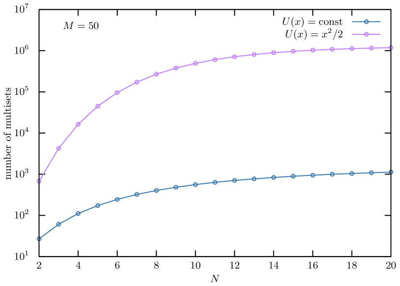
Figure 3: The number of multisets that must be considered assuming max_many_eig$\equiv M=50$ for the single-file in a flat (blue line) or in a harmonic (purple line) potential.

In Fig. 3 we show how many multisets must be considered for the convergence of the sum on a time-scale $\tau\gtrsim 1/\Lambda_{\mathbf{M}}$. Since these multisets are saved in std::vector<std::vector<int>> eigenfunction_store;, the size of this data structure prescribes the memory requirements of our program. The program saves these values to allow for a flexible way to compute the non-Markovian Green’s function (11) for the same system when tagging a different particle without the need to re-compute the necessary multisets. Though this number can become huge for some systems, for example in the case of the harmonic potential, it has been proved that for regular Sturm-Liouville problems the eigenvalues scale quadratically for large $k_{i}$ [35]. Since often also non-regular Sturm-Liouville problems on a infinite domain are treated numerically using truncation methods [36] our choice to save these numbers to enhance the flexibility and readability of the code is justified. Nevertheless, it would be equally possible not to save the necessary multisets and instead do all calculations on-the-fly.

Moreover, according to the specific properties of the Fokker-Planck operator $\hat{L}_{N}$ we sometimes find that $V_{\mathbf{k}\mathbf{0}}(x)=V_{\mathbf{0}\mathbf{k}}(x)$. A a result both functions can be implemented in terms of a single function responsible for $V_{\mathbf{k}\mathbf{l}}(x)$ without the necessity of code duplication. However, for the single-file in a linear potential this is not the case [10]. For this reason the functions for calculating the ’overlaps’ (i.e. Eqs. (12)) with the ground state are virtual, such that they can be implemented without re-factoring the code. In our implementation of class SingleFileOnSlope; the function Vk0_element is overridden with a marginally faster version to take into account the asymmetry of the single-file in a linear potential.

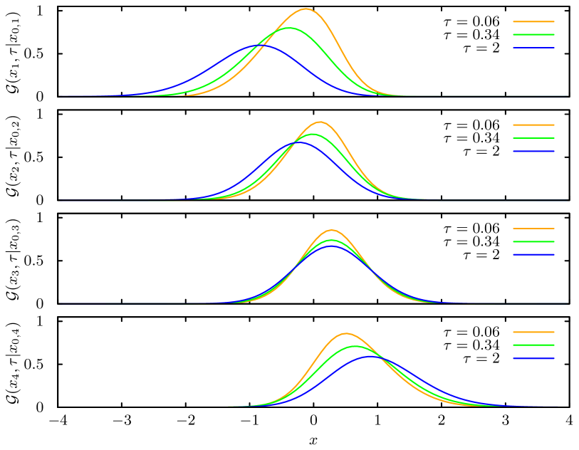
Figure 4: The tagged-particle Green’s function for different particles of a single-file of $4$ particles in a harmonic potential $U(x)=x^{2}/2$ at different times (the relaxation time is $\sim\lambda_{1}^{-1}=1$). Each particle’s initial position is $x_{0}=0.305$ assuming that all the other particles are in their respective equilibrium conditioned on the position of the tagged-particle.

In order to illustrate our final result we depict in Fig. 4 the computed Green’s function for a single-file of $4$ particles in a harmonic potential $U(x)=x^{2}/2$.

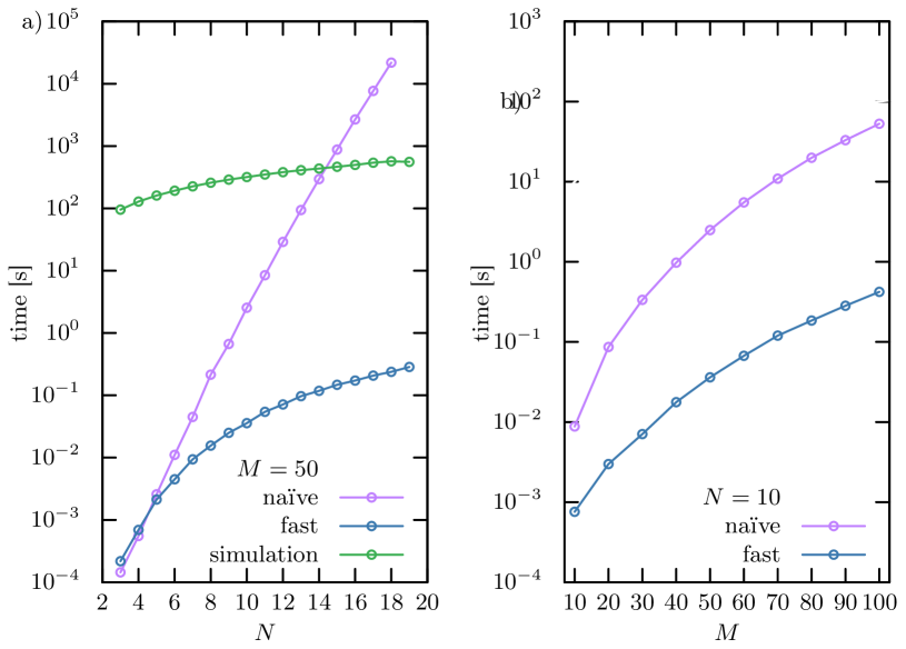
Figure 5: Computational time for calculating the tagged-particle Green’s function, in one specific space-time point a single-file in a flat potential. We compare our algorithm (blue lines) with the naïve implementation (purple lines) to a Brownian Dynamics simulation of $10^{4}$ trajectories with $2\times 10^{4}$ integration-steps of length $10^{-3}$ using Algorithm 2. In a) we fix the max many-body eigenvalue and tag the central particle while in b) we fix the total number of particles of the single-file and tag the fifth particle. For both plots the time to calculate all the available multisets in Eq. (5) has not been taken into account since it is the same the naïve and efficient implementations of the CBA solution.

Exceptions

Two classes for managing exceptions:
class NotImplementedException : public std::logic_error; and
class NotAllowedParameters : public std::logic_error; are included in the code base. The former allows to write a partially implemented derived class, while the latter just throws in the case that an ill-posed parameter is provided. All exceptions throw without any attempt to catch them.

Parallelization

By construction the evaluation of Eq. (5) for different $x,\tau$ and $x_{0}$ is parallelizable. A non-trivial parallelization may be achieved implementing a reduction for Eq. (5). However, for many systems (see Fig. 3) the number of terms in the sum is relatively small and a parallel approach is unnecessary unless the single-file is very big and/or we are interested in very small time-scales. The present code does not support parallelization and thread-safety is not guaranteed.

5 Comparison with Brownian Dynamics simulations

A fair comparison between our algorithm implementing a solution based on Eq. (11) and a Brownian Dynamics simulation integrating the Langevin equation (2) numerically is somewhat tricky. The reason is that the computational effort of a Brownian Dynamics simulation grows “forward” in time, while the eigenexpansion solution becomes challenging “backward” in time. In the former case the longer the time-scale we are interested in the more integration steps we must perform, while if we are interested in shorter time-scales a smaller integration time-step must be used. In the implementation of the Bethe ansazt solution in Eq. (11) we need to consider more and more terms in the sum over Bethe eigenvalues $\Lambda_{\mathbf{k}}$ in order to obtain reliable results for shorter time-scales. In contrast, essentially only two terms (i.e. the ground state $\Lambda_{\mathbf{0}}$ and the first excited state $\Lambda_{\mathbf{1}}$) are required if we are interested only in the long-time dynamics, i.e. $t>1/\Lambda_{\mathbf{1}}$.

In Algorithm 2 we present a convenient method to simulate single-file diffusion based on the Jepsen mapping [2]. The key step is the sorting of the particles’ positions (step 6) that allows avoiding a costly chain of if statements required to implement non-crossing conditions. To perform this step we use the sorting routine std::sort included in the C++ standard library. A comparison of this algorithm with the analytical solution can be found in [9].

Algorithm 2 Brownian Dynamics simulation of a single-file

1:.

• number of particles $N$;

• time-step $\Delta t$, final time $t_{f}$, list of sampling times $t_{s}$;

• number of trajectories $N_{t}$;

• the initial position of the tagged-particle $x_{0}$;

• a function to update a histogram.

2:for $i$=1:$N_{t}$ do

3:     $t\leftarrow 0$;

4:     Generate the initial position for the $N-1$ particle from their equilibrium distribution conditioned on the position of the tagged-particle $x_{0}$;

5:     while $t\leq t_{f}$ do

6:         Integrate the Langevin equation (using a Euler-Mayurama scheme for example) of $N$ independent particles using the time-step $\Delta t$;

7:         Sort in ascending order the particles’ positions to satisfy the non-crossing condition;

8:         if  $t\in t_{s}$ then

9:              Update the histogram containing the Green’s function of the tagged-particle;

10:         end if

11:         $t+=\Delta t$;

12:     end while

13:end for

14:return the histogram;

In Fig. 5 we present the computational time required to evaluate the Green’s function in a single point in space and time fixing either the maximum eigenvalue (panel a) or the number of particles (panel b). In the left panel we also plot the time required to compute the tagged-particle Green’s function of the single-file in a flat potential for different number of particles $N$ by means of a Brownian Dynamics simulation. We simulate $10^{4}$ trajectories with a time-step of $10^{-3}$ until time $t_{f}=20\approx 2/\Lambda_{\mathbf{1}}$ to ensure that the final equilibrium distribution is reached. Using these parameters the statistical error of the simulation is $\sim 5\%-10\%$ using $10^{4}$ trajectories and $1\%-2\%$ if instead we generate $10^{5}$ trajectories, in agreement with the Gaussian central limit theorem. Note that since we are considering enough terms in the series expansion (11) the analytic solution may be reliably considered to be exact on the time-scale of interest. Because the error of the Brownian Dynamics simulation can be reduced by increasing the number of independent trajectories, $N_{\rm traj}$, and since Algorithm 2 scales linearly with $N_{\rm traj}$, it is easy to extrapolate from Fig. 5 the computational effort required to obtain more accurate results.

Conversely, if we are interested only in short time-scales we must carry out the numerical integration of Eq. (2) for a small number (say $\sim 100$) of steps and thereby obtain better results (and with less computational effort) than the analytic solution. This is so because the analytical solution suffers from the Runge-phenomenon for short times, since we are approaching a delta-function distribution. However, such very short time-scales are less interesting since the tagged-particle behaves like a free-particle for times shorter the the average collision-time with neighboring particles [7]. For the same reason a smaller integration time-step must also be taken to capture all the non-trivial physics in a Brownian Dynamics simulation if we consider a single-file with a large number of particles $N$. In addition, if the Green’s function of the tagged-particle is peaked, the binning of the histogram in the analysis of simulations must be made sufficiently small, which imposes additional constraints on the integration time-step in order to obtain reliable results.

6 Conclusions

We presented an efficient numerical implementation of the exact coordinate Bethe ansatz solution of the non-Markovian tagged-particle propagator in a single-file in a general confining potential. Motivated by the fact that the Bethe eigenspectrum solution nominally carries a large computational cost when the number of particles is large we developed an efficient algorithm, which enables investigations of tagged-particle diffusion on a broad span of time-scales and for various numbers of particles. Our code exploits exchange symmetries in order to reduce the number of combinatorial operations. One of the main advantages of the Bethe ansatz solution, aside from the fact that it provides an exact solution of the problem and that it ties the tagged-particle dynamics to many-body relaxation eigenmodes, is that it is easy to generalize to take into account for any confining external potential or initial condition. For this reason we provide a header file SingleFileBluePrint.hpp that allows an easy extension of our codebase. With this goal in mind the expressiveness and the tools of modern C++ were used to achieve modularity and simplicity of use. The code can be easily extended in order to allow for a calculation of other key quantities related to the non-Markovian dynamics of a tagged-particle, e.g. the mean square displacement [31] as well as local-time statistics and other local additive functionals of tagged-particle trajectories [9, 10].

Appendix A Combinantorics

Permutations

Let $\mathbf{k}$ be a multiset of $N$ elements. Let $r_{i}$ denote the multiplicity of each of the $m$ distinct elements of $\mathbf{k}$ such that $\sum_{i=1}^{m}r_{i}=N$. Then the number of distinct permutations of this multiset is

$$\binom{N}{r_{1},r_{2},\cdots,r_{m}}=\frac{N!}{\prod_{i=1}^{m}r_{i}!}.$$ (21)

The denominator of Eq. (21) is what we call the multiplicity $m_{\mathbf{k}}$ of the multiset $\mathbf{k}$. For example, the distinct permutations of $\{1,1,2,3\}$ are: $\{\{1,1,2,3\}$, $\{1,1,3,2\}$, $\{1,2,1,3\}$, $\{1,2,3,1\}$, $\{1,3,1,2\}$, $\{1,3,2,1\}$,$\{2,1,1,3\}$, $\{2,1,3,1\}$, $\{2,3,1,1\}$, $\{3,1,1,2\}$, $\{3,1,2,1\}$, $\{3,2,1,1\}\}$.

$t$-combinations

The problems of enumerating and computing the combinations of a multiset can be mapped to the equivalent bounded composition problems [32]. James Bernoulli in 1713 enumerated them for the first time, observing that the number of the $t$-combinations of a multiset $\mathbf{k}$ with $m$ distinct elements, where each of them is contained $r_{m}$ times, is equal to the $t$-th coefficient of the polynomial $P_{\mathbf{k}}(z)$:

$$P_{\mathbf{k}}(z)=\prod_{i=1}^{m}p_{i}(z)$$ (22)

$$p_{i}(z)=\sum_{j=0}^{r_{i}}z^{j}.$$ (23)

For example the $2$-combinations of $\{1,1,1,2,3\}$ are: $\{\{1,1\}$, $\{1,2\}$, $\{1,3\}$, $\{2,3\}\}$.

Integer partitions

We refer to the integer partition of a number $N$ in $m$ parts as the number of ways in which $N$ can be expressed as a sum of all the numbers smaller or equal to itself. For example for $N=4$ and $m=4$: $\{0,0,0,4\}$,$\{0,0,1,3\}$,$\{0,0,2,2\}$,$\{0,1,1,2\}$,$\{1,1,1,1\}$.

Appendix B Single-particle eigenspectra

The dynamics of a single Brownian particle in a unit box in a constant potential with reflecting external boundary conditions is governed by the Sturm-Liouville problem

$$(\partial_{\tau}-D\partial^{2}_{x})\Gamma(x,\tau|x_{0})=0,$$

$$\partial_{x}\Gamma|_{x=0}=\partial_{x}\Gamma|_{x=1}=0$$ (24)

with the initial condition $\Gamma(x,0|x_{0})=\delta(x-x_{0})$. The corresponding Green’s function can be expressed in terms of a spectral expansion

$$\Gamma(x,\tau|x_{0})=\sum_{k}\psi^{R}_{k}(x)\psi^{L}_{k}(x_{0})\mathrm{e}^{-\lambda_{k}\tau},$$ (25)

where

$$\psi^{L}_{0}(x)=\psi^{R}_{0}(x)=1,$$ (26)

$$\psi^{L}_{k}(x)=\psi^{R}_{k}(x)=\sqrt{2}\cos(k\pi x),$$ (27)

$$\lambda_{k}=k^{2}\pi^{2}.$$ (28)

On the other hand, if we add a linear potential the corresponding Fokker-Planck equation for the Green’s function becomes

$$(\partial_{\tau}-D\partial^{2}_{x}-g\partial_{x})\Gamma(x,\tau|x_{0})=0,$$ (29)

with initial condition $\Gamma(x,0|x_{0})=\delta(x-x_{0})$, and the eigenexpansion is given by

$$\lambda_{0}=0,$$ (30)

$$\lambda_{k}=Dk^{2}\pi^{2}+\frac{g^{2}}{4D},$$ (31)

$$\psi^{L}_{0}(x)=1,$$ (32)

$$\psi^{L}_{k}(x)=\displaystyle{\frac{\mathrm{e}^{\frac{gx}{2D}}}{\sqrt{1/2+2Dk^{2}\pi^{2}/g^{2}}}}(\sin(k\pi x)-2Dk\pi\cos(k\pi x)/g),$$ (33)

$$\psi^{R}_{0}(x)=\displaystyle{\frac{g}{D}\frac{\mathrm{e}^{-\frac{gx}{D}}}{1-\mathrm{e}^{-\frac{g}{D}}}},$$ (34)

$$\psi^{R}_{k}(x)=\displaystyle{\frac{\mathrm{e}^{-\frac{gx}{2D}}}{\sqrt{1/2+2Dk^{2}\pi^{2}/g^{2}}}}(\sin(k\pi x)-2Dk\pi\cos(k\pi x)/g).$$ (35)

Finally for an Ornstein-Uhlenbeck process with natural boundary conditions (i.e. $\lim_{|x|\to\infty}\Gamma(x,\tau|x_{0})=0$) the Green’s function is given by

$$(\partial_{\tau}-D\partial^{2}_{x}-\gamma\partial_{x}x)\Gamma(x,\tau|x_{0})=0,$$ (37)

with initial condition $\Gamma(x,0|x_{0})=\delta(x-x_{0})$ and eigenexpansion

$$\psi^{L}_{k}(x)=\displaystyle{\frac{1}{\sqrt{2^{k}k!}}}H_{k}(x\sqrt{\gamma/2D})$$ (38)

$$\psi^{R}_{k}(x)=\displaystyle{\sqrt{\frac{\gamma}{2\pi D}}}\mathrm{e}^{-\frac{\gamma x^{2}}{2D}}\psi^{L}_{k}(x)$$ (39)

$$\lambda_{k}=\gamma k,$$ (40)

where $H_{k}(x)$ denotes the $k$th “physicist’s” Hermite polynomial [37].

References

- [1] T. E. Harris, Diffusion with “collisions” between particles, Journal of Applied Probability 2 (2) (1965) 323–338. doi:10.2307/3212197.
-
[2]
D. W. Jepsen, Dynamics of
a Simple Many‐Body System of Hard Rods, Journal of
Mathematical Physics 6 (3) (1965) 405–413.
doi:10.1063/1.1704288.
URL http://aip.scitation.org/doi/10.1063/1.1704288 -
[3]
H. van Beijeren,
Fluctuations in the
motions of mass and of patterns in one-dimensional driven diffusive systems,
J Stat Phys 63 (1-2) (1991) 47–58.
doi:10.1007/BF01026591.
URL http://link.springer.com/10.1007/BF01026591 -
[4]
C. Rödenbeck, J. Kärger, K. Hahn,
Calculating exact
propagators in single-file systems via the reflection principle, Phys. Rev.
E 57 (4) (1998) 4382–4397.
doi:10.1103/PhysRevE.57.4382.
URL https://link.aps.org/doi/10.1103/PhysRevE.57.4382 -
[5]
E. Barkai, R. Silbey,
Theory of
Single File Diffusion in a Force Field, Phys. Rev. Lett. 102 (5)
(2009) 050602.
doi:10.1103/PhysRevLett.102.050602.
URL https://link.aps.org/doi/10.1103/PhysRevLett.102.050602 -
[6]
T. Ambjörnsson, L. Lizana, M. A. Lomholt, R. J. Silbey,
Single-file dynamics
with different diffusion constants, J. Chem. Phys. 129 (18) (2008) 185106.
doi:10.1063/1.3009853.
URL https://aip.scitation.org/doi/10.1063/1.3009853 -
[7]
L. Lizana, T. Ambjörnsson,
Single-File
Diffusion in a Box, Phys. Rev. Lett. 100 (20) (2008) 200601.
doi:10.1103/PhysRevLett.100.200601.
URL https://link.aps.org/doi/10.1103/PhysRevLett.100.200601 -
[8]
L. Lizana, T. Ambjörnsson, A. Taloni, E. Barkai, M. A. Lomholt,
Foundation of
fractional Langevin equation: Harmonization of a many-body problem,
Phys. Rev. E 81 (5) (2010) 051118.
doi:10.1103/PhysRevE.81.051118.
URL https://link.aps.org/doi/10.1103/PhysRevE.81.051118 - [9] A. Lapolla, A. Godec, Unfolding tagged particle histories in single-file diffusion: exact single- and two-tag local times beyond large deviation theory, New J. Phys. 20 (11) (2018) 113021.
-
[10]
A. Lapolla, A. Godec,
Manifestations
of Projection-Induced Memory: General Theory and the Tilted
Single File, Front. Phys. 7.
doi:10.3389/fphy.2019.00182.
URL https://www.frontiersin.org/articles/10.3389/fphy.2019.00182/full -
[11]
C. Lutz, M. Kollmann, C. Bechinger,
Single-File
Diffusion of Colloids in One-Dimensional Channels, Phys. Rev.
Lett. 93 (2) (2004) 026001.
doi:10.1103/PhysRevLett.93.026001.
URL https://link.aps.org/doi/10.1103/PhysRevLett.93.026001 -
[12]
B. Lin, M. Meron, B. Cui, S. A. Rice, H. Diamant,
From Random
Walk to Single-File Diffusion, Phys. Rev. Lett. 94 (21) (2005)
216001.
doi:10.1103/PhysRevLett.94.216001.
URL https://link.aps.org/doi/10.1103/PhysRevLett.94.216001 -
[13]
E. Locatelli, M. Pierno, F. Baldovin, E. Orlandini, Y. Tan, S. Pagliara,
Single-File
Escape of Colloidal Particles from Microfluidic Channels, Phys.
Rev. Lett. 117 (3) (2016) 038001.
doi:10.1103/PhysRevLett.117.038001.
URL https://link.aps.org/doi/10.1103/PhysRevLett.117.038001 -
[14]
G. Hummer, J. C. Rasaiah, J. P. Noworyta,
Water conduction through the
hydrophobic channel of a carbon nanotube, Nature 414 (6860) (2001) 188–190.
doi:10.1038/35102535.
URL http://www.nature.com/articles/35102535 - [15] S. Ahlberg, T. Ambjörnsson, L. Lizana, Many-body effects on tracer particle diffusion with applications for single-protein dynamics on DNA, New Journal of Physics 17 (4) (2015) 043036. doi:10.1088/1367-2630/17/4/043036.
-
[16]
T. Chou, D. Lohse,
Entropy-Driven
Pumping in Zeolites and Biological Channels, Phys. Rev. Lett.
82 (17) (1999) 3552–3555.
doi:10.1103/PhysRevLett.82.3552.
URL https://link.aps.org/doi/10.1103/PhysRevLett.82.3552 - [17] J. Kärger, D. M. Ruthven, Diffusion in zeolites and other microporous solids, A Wiley Interscience publication, Wiley, New York, 1992, oCLC: 22451684.
-
[18]
P. M. Richards, Theory
of one-dimensional hopping conductivity and diffusion, Phys. Rev. B 16 (4)
(1977) 1393–1409.
doi:10.1103/PhysRevB.16.1393.
URL https://link.aps.org/doi/10.1103/PhysRevB.16.1393 -
[19]
A. Taloni, O. Flomenbom, R. Castañeda-Priego, F. Marchesoni,
Single file dynamics in soft
materials, Soft Matter 13 (6) (2017) 1096–1106.
doi:10.1039/C6SM02570F.
URL http://xlink.rsc.org/?DOI=C6SM02570F -
[20]
X. Hu, L. Hong, M. Dean Smith, T. Neusius, X. Cheng, J. Smith,
The dynamics of single protein
molecules is non-equilibrium and self-similar over thirteen decades in time,
Nat. Phys. 12 (2) (2015) 171–174.
doi:10.1038/nphys3553.
URL http://dx.doi.org/10.1038/nphys3553 -
[21]
K. Henzler-Wildman, D. Kern,
Dynamic personalities of
proteins, Nature 450 (7172) (2007) 964–972.
doi:10.1038/nature06522.
URL http://www.nature.com/articles/nature06522 -
[22]
G.-W. Li, O. G. Berg, J. Elf,
Effects of macromolecular
crowding and DNA looping on gene regulation kinetics, Nat. Phys. 5 (4)
(2009) 294–297.
doi:10.1038/nphys1222.
URL http://www.nature.com/articles/nphys1222 -
[23]
E. Barkai, R. Silbey,
Diffusion of
tagged particle in an exclusion process, Phys. Rev. E 81 (4) (2010) 041129.
doi:10.1103/PhysRevE.81.041129.
URL https://link.aps.org/doi/10.1103/PhysRevE.81.041129 -
[24]
N. Leibovich, E. Barkai,
Everlasting effect
of initial conditions on single-file diffusion, Phys. Rev. E 88 (3) (2013)
032107.
doi:10.1103/PhysRevE.88.032107.
URL https://link.aps.org/doi/10.1103/PhysRevE.88.032107 - [25] Korepin, V E, Bogoliubov, N M, Izergin, A G, Quantum Inverse Scattering Method and Correlation Functions, Cambridge Monographs on Mathematical Physics, Cambridge University Press, 1997.
- [26] A. Lapolla, A. Godec, Faster uphill relaxation in equidistant temperature quenches (2020). arXiv:2002.08237.
-
[27]
S. Herrera-Velarde, R. Castañeda-Priego,
Superparamagnetic
colloids confined in narrow corrugated substrates, Phys. Rev. E 77 (4)
(2008) 041407.
doi:10.1103/PhysRevE.77.041407.
URL https://link.aps.org/doi/10.1103/PhysRevE.77.041407 -
[28]
S. Herrera-Velarde, G. Pérez-Angel, R. Castañeda-Priego,
One-dimensional Gaussian-core
fluid: ordering and crossover from normal diffusion to single-file dynamics,
Soft Matter 12 (44) (2016) 9047–9057.
doi:10.1039/C6SM01558A.
URL http://xlink.rsc.org/?DOI=C6SM01558A - [29] L. Chupin, Fokker-Planck equation in bounded domain, Ann. inst. Fourier 60 (1) (2010) 217–255. doi:10.5802/aif.2521.
-
[30]
J. Kurchan, Six out of equilibrium
lectures, arXiv:0901.1271 [cond-mat]ArXiv: 0901.1271.
URL http://arxiv.org/abs/0901.1271 -
[31]
L. Lizana, T. Ambjörnsson,
Diffusion of
finite-sized hard-core interacting particles in a one-dimensional box:
Tagged particle dynamics, Phys. Rev. E 80 (5) (2009) 051103.
doi:10.1103/PhysRevE.80.051103.
URL https://link.aps.org/doi/10.1103/PhysRevE.80.051103 - [32] D. E. Knuth, The Art of Computer Programming, 4th Edition, Vol. 4a, Addison-Wesley, 2013.
- [33] Gardiner, C.W., Handbook of Stochastic Methods for Physics, Chemistry and Natural Sciences, 2nd Edition, Springer-Verlag, 1985.
-
[34]
H. Risken, T. Frank, The
Fokker-Planck Equation: Methods of Solution and Applications,
2nd Edition, Springer Series in Synergetics, Springer-Verlag, Berlin
Heidelberg, 1996.
doi:10.1007/978-3-642-61544-3.
URL https://www.springer.com/gp/book/9783540615309 -
[35]
H. Hochstadt,
Asymptotic
estimates for the Sturm-Liouville spectrum, Commun. Pur. Aappl. Math.
14 (4) (1961) 749–764.
doi:10.1002/cpa.3160140408.
URL https://onlinelibrary.wiley.com/doi/abs/10.1002/cpa.3160140408 - [36] J. P. Boyd, Chebyshev and Fourier Spectral Methods, Dover, New York, 2001.
- [37] Abramowitz, Milton and Stegun, Irene A., Handbook of Mathematical Functions with Formulas, Graphs, and Mathematical Tables, ninth dover printing, tenth gpo printing Edition, Dover, New York, 1964.