Computational Complexity of the $\alpha$-Ham-Sandwich Problem

Abstract

The classic Ham-Sandwich theorem states that for any $d$ measurable sets in $\mathbb{R}^{d}$, there is a hyperplane that bisects them simultaneously. An extension by Bárány, Hubard, and Jerónimo  [DCG 2008] states that if the sets are convex and well-separated, then for any given $\alpha_{1},\dots,\alpha_{d}\in[0,1]$, there is a unique oriented hyperplane that cuts off a respective fraction $\alpha_{1},\dots,\alpha_{d}$ from each set. Steiger and Zhao [DCG 2010] proved a discrete analogue of this theorem, which we call the $\alpha$-Ham-Sandwich theorem. They gave an algorithm to find the hyperplane in time $O(n(\log n)^{d-3})$, where $n$ is the total number of input points. The computational complexity of this search problem in high dimensions is open, quite unlike the complexity of the Ham-Sandwich problem, which is now known to be $\mathsf{PPA}$-complete (Filos-Ratsikas and Goldberg [STOC 2019]).

Recently, Fearley, Gordon, Mehta, and Savani [ICALP 2019] introduced a new sub-class of $\mathsf{CLS}$ (Continuous Local Search) called Unique End-of-Potential Line ($\mathsf{UEOPL}$). This class captures problems in $\mathsf{CLS}$ that have unique solutions. We show that for the $\alpha$-Ham-Sandwich theorem, the search problem of finding the dividing hyperplane lies in $\mathsf{UEOPL}$. This gives the first non-trivial containment of the problem in a complexity class and places it in the company of classic search problems such as finding the fixed point of a contraction map, the unique sink orientation problem and the $P$-matrix linear complementarity problem.

1 Introduction

Motivation and related work.

The Ham-Sandwich Theorem [ST42] is a classic result about partitioning sets in high dimensions: for any $d$ measurable sets $S_{1},\dots,S_{d}\subset\mathbb{R}^{d}$ in $d$ dimensions, there is an oriented hyperplane $H$ that simultaneously bisects $S_{1},\dots,S_{d}$. More precisely, if $H^{+},H^{-}$ are the closed half-spaces bounded by $H$, then for $i=1,\dots,d$, the measure of $S_{i}\cap H^{+}$ equals the measure of $S_{i}\cap H^{-}$. The traditional proof goes through the Borsuk-Ulam Theorem [Mat03]. The Ham-Sandwich Theorem is a cornerstone of geometry and topology, and it has found applications in other areas of mathematics, e.g., for the study of majority rule voting and the analysis of the stability of bicameral legislatures in social choice theory [CM84].

Let $[n]=\{1,\dots,n\}$. The discrete Ham-Sandwich Theorem [Mat03, LMS94] states that for any $d$ finite point sets $P_{1},\dots,P_{d}\subset\mathbb{R}^{d}$ in $d$ dimensions, there is an oriented hyperplane $H$ such that $H$ bisects each $P_{i}$, i.e., for $i\in[d]$, we have $\min\{|P_{i}\cap H^{+}|,|P_{i}\cap H^{-}|\}\geq\left\lceil|P_{i}|/2\right\rceil$. We denote the associated search problem as Ham-Sandwich. Lo, Matoušek, and Steiger [LMS94] gave an $n^{O(d)}$-time algorithm for Ham-Sandwich. They also provided a linear-time algorithm for points in $\mathbb{R}^{3}$, under additional constraints.

There are many alternative and more general variants of both the continuous and the discrete Ham-Sandwich Theorem. For example, Bárány and Matoušek [BM01] derived a version where measures in the plane can be divided into any (possibly different) ratios by fans instead of hyperplanes (lines). A discrete variant of this result was given by Bereg [Ber05]. Schnider [Sch19a] studied a generalization in higher dimensions. Recently Barba, Pilz, and Schnider [BPS19] showed that four measures in the plane can be bisected with two lines. Zivaljević and Vrećica [ZV90] proved a result that interpolates between the Ham-Sandwich Theorem and the Centerpoint Theorem [Rad46], of which there is also a no-dimensional version [CM20]. Schnider [Sch19b] presented a generalization based on this result among others.

Here, we focus on a version that allows for dividing the sets into arbitrary given ratios instead of simply bisecting them. The sets $S_{1},\dots,S_{d}\subset\mathbb{R}^{d}$ are well-separated if every selection of them can be strictly separated from the others by a hyperplane. Bárány, Hubard, and Jerónimo [BHJ08] showed that if $S_{1},\dots,S_{d}$ are well-separated and convex, then for any given reals $\alpha_{1},\dots,\alpha_{d}\in[0,1]$, there is a unique hyperplane that divides $S_{1},\dots,S_{d}$ in the ratios $\alpha_{1},\dots,\alpha_{d}$, respectively. Their proof goes through Brouwer’s Fixed Point Theorem. Steiger and Zhao [SZ10] formulated a discrete version. In this setup, $S_{1},\dots,S_{d}$ are finite point sets. Again, we need that the (convex hulls of the) $S_{i}$ are well-separated. Additionally, we require that the $S_{i}$ follow a weak version of general position. Let $\alpha_{1},\dots,\alpha_{d}\in\mathbb{N}$ be $d$ integers with $1\leq\alpha_{i}\leq|S_{i}|$, for $i\in[d]$. Then, there is a unique oriented hyperplane $H$ that passes through one point from each $S_{i}$ and has $|H^{+}\cap S_{i}|=\alpha_{i}$, for $i\in[d]$ [SZ10]. In other words, $H$ simultaneously cuts off $\alpha_{i}$ points from $S_{i}$, for $i\in[d]$. This statement does not necessarily hold if the sets are not well-separated, see Figure 1 for an example.

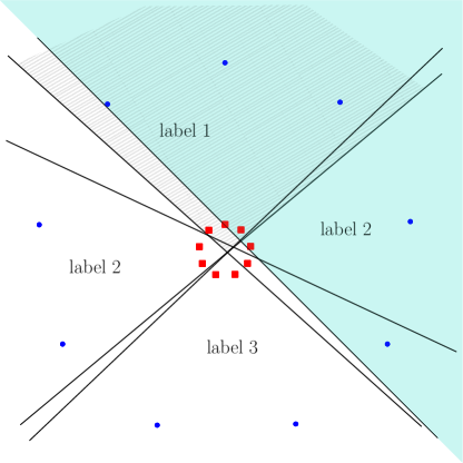
Figure 1: The red (square) and the blue (round) point sets are not well-separated. Every halfplane that contains three red points must contain at least five blue points. Thus, there is no halfplane that contains exactly three red and three blue points.

Steiger and Zhao called their result the Generalized Ham-Sandwich Theorem, yet it is not a strict generalization of the classic Ham-Sandwich Theorem. Their result requires that the point sets obey well-separation and weak general position, while the classic theorem always holds without these assumptions. Therefore, we call this result the $\alpha$-Ham-Sandwich theorem, for a clearer distinction. Set $n=\sum_{i\in[d]}|S_{i}|$. Steiger and Zhao gave an algorithm that computes the dividing hyperplane in $O\left(n(\log n)^{d-3}\right)$ time, which is exponential in $d$. Later, Bereg [Ber12] improved this algorithm to achieve a running time of $n2^{O(d)}$, which is linear in $n$ but still exponential in $d$. We denote the associated computational search problem of finding the dividing hyperplane as Alpha-HS.

No polynomial algorithms are known for Ham-Sandwich and for Alpha-HS if the dimension is not fixed, and the notion of approximation is also not well-explored. Despite their superficial similarity, it is not immediately apparent whether the two problems are comparable in terms of their complexity. Due to the additional requirements on an input for Alpha-HS, an instance of Ham-Sandwich may not be reducible to Alpha-HS in general.

Since a dividing hyperplane for Alpha-HS is guaranteed to exist if the sets satisfy the conditions of well-separation and (weak) general position, Alpha-HS is a total search problem. In general, such problems are modelled by the complexity class $\mathsf{TFNP}$ (Total Function Nondeterministic Polynomial) of $\mathsf{NP}$-search problems that always admit a solution. Two popular subclasses of $\mathsf{TFNP}$, originally defined by Papadimitriou [Pap94], are $\mathsf{PPA}$ (Polynomial Parity Argument) its sub-class $\mathsf{PPAD}$. These classes contain total search problems where the existence of a solution is based on a parity argument in an undirected or in a directed graph, respectively. Another sub-class of $\mathsf{TFNP}$ is $\mathsf{PLS}$ (polynomial local search). It models total search problems where the solutions can be obtained as minima in a local search process, while the number of steps in the local search may be exponential in the input size. The class $\mathsf{PLS}$ was introduced by Johnson, Papadimitriou, and Yannakakis [JPY88]. A noteworthy sub-class of $\mathsf{PPAD}\cap\mathsf{PLS}$ is $\mathsf{CLS}$ (continuous local search) [DP11]. It models similar local search problems over a continuous domain using a continuous potential function.

Up to very recently, these complexity classes have mostly been studied in the context of algorithmic game theory. However, there have been increasing efforts towards mapping the complexity landscape of existence theorems in high-dimensional discrete geometry. Computing an approximate solution for the search problem associated with the Borsuk-Ulam Theorem is in $\mathsf{PPA}$. In fact, this problem is complete for this class. The discrete analogue of the Borsuk-Ulam Theorem, Tucker’s Lemma [Tuc46], is also $\mathsf{PPA}$-complete [ABB20]. Therefore, since the traditional proof of the Ham-Sandwich Theorem goes through the Borsuk-Ulam Theorem, it follows that Ham-Sandwich lies in $\mathsf{PPA}$. In fact, Filos-Ratsikas and Goldberg [FRG19] recently showed that Ham-Sandwich is complete for $\mathsf{PPA}$. The (presumably smaller) class $\mathsf{PPAD}$ is associated with fixed-point type problems: computing an approximate Brouwer fixed point is a prototypical complete problem for $\mathsf{PPAD}$. The discrete analogue of Brouwer’s Fixed Point Theorem, Sperner’s Lemma, is also complete for $\mathsf{PPAD}$. In a celebrated result, the relevance of $\mathsf{PPAD}$ for algorithmic game theory was made clear when it turned out that computing a Nash-equilibrium in a two player game is $\mathsf{PPAD}$-complete [CDT09]. In discrete geometry, finding a solution to the Colorful Carathéodory problem [Bár82] was shown to lie in the intersection $\mathsf{PPAD}\cap\mathsf{PLS}$ [MMSS17, MS18]. This further implies that finding a Tverberg partition (and computing a centerpoint) also lies in the intersection [Tve66, Sar92, LGMM19]. The problem of computing the (unique) fixed point of a contraction map is known to lie in $\mathsf{CLS}$ [DP11].

Recently, at ICALP 2019, Fearley, Gordon, Mehta, and Savani defined a sub-class of $\mathsf{CLS}$ that represents a family of total search problems with unique solutions [FGMS19]. They named the class Unique End of Potential Line ($\mathsf{UEOPL}$) and defined it through the canonical complete problem UniqueEOPL. This problem is modelled as a directed graph. There are polynomially-sized Boolean circuits that compute the successor and predecessor of each node, and a potential value that always increases on a directed path. There is supposed to be only a single vertex with no predecessor (start of line). Under these conditions, there is a unique path in the graph that ends on a vertex (called end of line) with the highest potential along the path. This vertex is the solution to UniqueEOPL. Since the uniqueness of the solution is guaranteed only under certain assumptions, such a formulation is called a promise problem. Since there seems to be no efficient way to verify the assumptions, the authors allow two possible outcomes of the search algorithm: either report a correct solution, or provide any solution that was found to be in violation of the assumptions. This formulation turns UniqueEOPL into a non-promise problem and places it in $\mathsf{TFNP}$, since a correct solution is bound to exist when there are no violations, and otherwise a violation can be reported as a solution. Fearley et al. [FGMS19] also introduced the concept of a promise-preserving reduction between two problems $A$ and $B$, such that if an instance of $A$ has no violations, then the reduced instance of $B$ is also free of violations. This notion is particularly meaningful for non-promise problems.

Contributions.

We provide the first non-trivial containment in a complexity class for the $\alpha$-Ham-Sandwich problem by locating it in $\mathsf{UEOPL}$. More precisely, we formulate Alpha-HS as a non-promise problem in which we allow for both valid solutions representing the correct dividing hyperplane, as well as violations accounting for the lack of well-separation and/or (weak) general position of the input point sets. A precise formulation of the problem is given in Definition 4 in Section 2. We then show a promise-preserving reduction from Alpha-HS to UniqueEOPL. This implies that Alpha-HS lies in $\mathsf{UEOPL}$, and hence in $\mathsf{CLS}\subseteq\mathsf{PPAD}\cap\mathsf{PLS}$. See Figure 2 for a pictorial description.

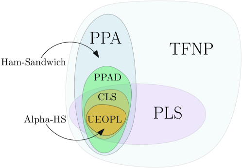
Figure 2: The hierarchy of complexity classes.

It is not surprising to discover that Alpha-HS lies in $\mathsf{PPAD}$, since the proof of the continuous version in [BHJ08] was based on Brouwer’s Fixed Point Theorem. The observation that it also lies in $\mathsf{PLS}$ is new and noteworthy, putting Alpha-HS into the reach of local search algorithms. In contrast, given our current understanding of total search problems, it is unlikely that the problem Ham-Sandwich would be in $\mathsf{PLS}$.

Since Alpha-HS lies in $\mathsf{PPAD}\subseteq\mathsf{PPA}$, it is computationally easier than Ham-Sandwich, which is $\mathsf{PPA}$-complete. This implies the existence of a polynomial-time reduction from Alpha-HS to Ham-Sandwich. A reduction in the other direction is unlikely. It thus turns out that well-separation brings down the complexity of the problem by a significant amount.

Often, problems in $\mathsf{TFNP}$ come in the guise of a polynomial-size Boolean circuit with some property. In contrast, Alpha-HS is a purely geometric problem that has no circuit in its problem definition. This is the second problem in $\mathsf{UEOPL}$ apart from the $P$-Matrix Linear complementarity problem and one of the few in $\mathsf{CLS}$ that does not have a description in terms of circuits.

Our local-search formulation is based on the intuition of rotating a hyperplane until we reach the desired solution. We essentially start with a hyperplane that is tangent to the convex hull of each input set, and we deterministically rotate the hyperplane until it hits a new point. This rotation can be continued whenever the hyperplane hits a new point, until we reach the correct dividing hyperplane. In other words, we can follow a local-search argument to find the solution. We show that this sequence of rotations can be modelled as a canonical path in a grid graph, and we give a potential function that guides the rotation and always increases along this path. Every violation of well-separation and (weak) general position can destroy this path. Furthermore, no efficient methods to verify these two assumptions are known. This poses a major challenge in handling the violations. One of our main technical contributions is to handle the violation solutions concisely.

An alternative approach would have been to look at the dual space of points where we get an arrangement of hyperplanes. The dividing hyperplane could then be found by looking at the correct level sets of the arrangement. However, this approach has the problem that the orientations of the hyperplanes in the original space and the dual space are not consistent. This complicates the arguments on the level sets, so we found it more convenient to use our notion of rotating hyperplanes. We show that we can maintain a consistent orientation throughout the rotation, and an inconsistent rotation is detected as a violation of the promise.

Outline of the paper.

We discuss the background about the $\alpha$-Ham-sandwich Theorem and UniqueEOPL in Section 2. In Section 3, we describe our instance of Alpha-HS and give an overview of the reduction and violation-handling. The technical details of the reduction are presented in Section 4 and Section 5. We conclude in Section 6.

2 Preliminaries

2.1 The $\bm{\alpha}$-Ham-Sandwich problem

For conciseness, we describe the discrete version of $\alpha$-Ham-Sandwich Theorem [SZ10] here. The continuous version [BHJ08] follows a similar formulation.

Let $P_{1},\dots,P_{d}\subset\mathbb{R}^{d}$ be a collection of $d$ finite point sets. Let $n_{1},\dots,n_{d}$ denote the sizes of $P_{1},\dots,P_{d}$, respectively. For each $i\in[d]$ we say that the point set $P_{i}$ represents a unique color and let $P:=P_{1}\cup\dots\cup P_{d}$ denote the union of all the points. A set of points $\{p_{1},\dots,p_{m}\}$ is said to be colorful if there are no two points $p_{i},p_{j}$ both from the same color. Indeed a colorful point set can have size at most $d$.

Weak general position.

We say that $P$ has very weak general position [SZ10], if for every choice of points $x_{1}\in P_{1},\dots,x_{d}\in P_{d}$, the affine hull of the set $\{x_{1},\dots,x_{d}\}$ is a $(d-1)$-flat and does not contain any other point of $P$. This definition is sufficient for the result of Steiger and Zhao, where they simply call it as weak general position. Of course, this definition of weak general position has no restriction on sets $\{x_{1},\dots,x_{d}\}$ that contain multiple points from the same color. To simplify our proofs we need a slightly stronger form of general position. We say that $P$ has weak general position if the above restriction also applies to sets having exactly $d-1$ colors. That means, each color may contribute at most one point to the set, except perhaps one color which is allowed to contribute two points. A certificate for checking violations of weak general position is a set of $d+1$ points whose affine hull has dimension at most $d-1$, with at least $d-1$ colors in the set. Testing whether a planar point set is in general position can be shown to be $\mathsf{NP}$-Hard, using the result in [FKNN17]. It is easy to see that when $d=2$, weak general position is equivalent to general position.

Well-separation.

The point set $P$ is said to be well-separated [SZ10, BHJ08], if for every choice of points $y_{1}\in\mathrm{conv}(P_{i_{1}}),\dots,y_{k}\in\mathrm{conv}(P_{i_{k}})$, where $i_{1},\dots,i_{k}$ are distinct indices and $1\leq k\leq d+1$, the affine hull of $\{y_{1},\dots,y_{k}\}$ is a $(k-1)$-flat. An equivalent definition is as follows: $P$ is well-separated if and only if for every disjoint pair of index sets $I,J\subset[d]$, there is hyperplane that separates the set $\{\cup_{i\in I}P_{i}\}$ from the set $\{\cup_{j\in J}P_{j}\}$ strictly. Formally:

Lemma 1.

Let $y_{1},\dots,y_{d}$ be a colorful set of points in the corresponding $\mathrm{conv}(P_{i})$. The affine hull of $y_{1},\dots,y_{d}$ has dimension $d-2$ or less if and only if there is a partition of $[d]$ into index sets $I,J$ such that $\mathrm{conv}\left(\{\cup_{i\in I}P_{i}\}\right)\cap\mathrm{conv}\left(\{\cup_{j\in J}P_{j}\}\right)\neq\emptyset$.

Given such a colorful set, the partition of $[d]$ can be computed in $\mathrm{poly}(n,d)$ time. Vice-versa, given such a partition, the colorful set can be computed in $\mathrm{poly}(n,d)$ time.

Proof.

First we prove the reverse implication: we are given $y_{1},\dots,y_{d}$, and the affine hull has dimension at most $d-2$. By Radon’s theorem [Rad21] there is a partition of $y_{1},\dots,y_{d}$ into two sets $\{y_{i_{1}},\dots,y_{i_{m}}\}$ and $\{y_{j_{1}},\dots,y_{j_{d-m}}\}$ such that their convex hulls intersect in some point $z\in\mathbb{R}^{d}$. Then for the sets $I=\{i_{1},\dots,i_{m}\},J=\{j_{1},\dots,j_{d-m}\}$, we have that $z\in\mathrm{conv}(\{\cup_{i\in I}P_{i}\})\cap\mathrm{conv}(\{\cup_{j\in J}P_{j}\})$. Furthermore, the Radon partition (and hence the partition of $[d]$) can be computed in $O(d^{3})$ time by solving a system of linear equations [Mat02]. This proves the first part of the claim.

For the other direction, we first use linear programming to find a point $z$ in the intersection of $\mathrm{conv}(\{\cup_{i\in I}P_{i}\})$ and $\mathrm{conv}(\{\cup_{j\in J}P_{j}\})$. Using Carathéodory’s Theorem [Car07], there exists a subset $Q=\{p_{1},\ldots,p_{d+1}\}\subset\{\cup_{i\in I}P_{i}\}$ of $d+1$ points such that $z\in\mathrm{conv}(Q)$. Let $c_{1}$ be the number of colors in $Q$. We shrink $Q$ so that it contains one point from the convex hull of each color. Since $\mathrm{conv}(Q)$ is a $d$-simplex, $\mathrm{conv}(Q)$ contains an edge for every pair of points $(p_{i},p_{j})$. For $(p_{i},p_{j})$ with the same color $t$, we shrink the edge $(p_{i},p_{j})$ to a point $x_{t}\in\mathrm{conv}(P_{t})$ such that $z$ stays inside $\mathrm{conv}\left(Q\cup\{x_{t}\}\setminus\{p_{i},p_{j}\}\right)$. In this process $Q:=Q\cup\{x_{t}\}\setminus\{p_{i},p_{j}\}$ shrinks to a $(d-1)$-simplex. We repeat this process until all points of $Q$ with color $t$ are shrunk to a single point. We continue this process for the remaining colors, ending at a simplex $S_{1}$ of dimension $c_{1}-1$. We apply the same procedure for $z\in\mathrm{conv}(\{\cup_{j\in J}P_{j}\})$ to obtain another simplex $S_{2}$ of dimension $c_{2}-1$. Since $z\in S_{1}\cap S_{2}$, the lowest dimension of a flat containing $S_{1}$ and $S_{2}$ is at most $c_{1}+c_{2}-2\leq d-2$. For each color not in $S_{1}$ and $S_{2}$, we select an arbitrary point for each, then $S_{1}$, $S_{2}$ and the chosen points span a $(d-2)$-flat. $Q$ can be computed in polynomial time [LGMM19, Mat02] along with the other steps in the construction. Therefore, the colorful set can be computed in polynomial time, proving our claim. ∎

A certificate for checking violations of well-separation is a colorful set $\{x_{1},\dots,x_{d}\}$ whose affine hull has dimension at most $d-2$. Another certificate is a partition $I,J\subset[d]$ such that the convex hulls of the indexed sets are not separable. Due to Lemma 1, both certificates are equivalent and either can be converted to the other in polynomial time. To the best of our knowledge, the complexity of testing well-separation is unknown.

Given any set of positive integers $\{\alpha_{1},\dots,\alpha_{d}\}$ satisfying $1\leq\alpha_{i}\leq n_{i}$, $i\in[d]$, an $(\alpha_{1},\dots,\alpha_{d})$-cut is an oriented hyperplane $H$ that contains one point from each color and satisfies $|H^{+}\cap P_{i}|=\alpha_{i}$ for $i\in[d]$, where $H^{+}$ is the closed positive half-space defined by $H$.

Theorem 2 ($\alpha$-Ham-Sandwich Theorem [SZ10]).

Let $P_{1},\ldots,P_{d}$ be finite, well-separated point sets in $\mathbb{R}^{d}$. Let $\alpha=(\alpha_{1},\dots,\alpha_{d})$ be a vector, where $\alpha_{i}\in[n_{i}]$ for $i\in[d]$.

1. If an $\alpha$-cut exists, then it is unique.

2. If $P$ has weak general position, then a cut exists for each choice of $\alpha$, $\alpha_{i}\in[n_{i}]$.

That means, every colorful $d$-tuple of $P$ corresponds to exactly one $\alpha$-vector. Steiger and Zhao [SZ10] also presented an algorithm to compute the cut in $O(n(\log n)^{d-3})$ time, where $n=\sum_{i=1}^{d}n_{i}$. The algorithm proceeds inductively in dimension and employs a prune-and-search technique. Bereg [Ber12] improved the pruning step to improve the runtime to $n2^{O(d)}$.

2.2 Unique End of Potential Line

We briefly explain the Unique end of potential line problem that was introduced in [FGMS19]. More details about the problem and the associated class can be found in the above reference.

Definition 3 (from[FGMS19]).

Let $n,m$ be positive integers. The input consists of

• a pair of Boolean circuits $\mathbb{S},\mathbb{P}:\{0,1\}^{n}\rightarrow\{0,1\}^{n}$ such that $\mathbb{P}(0^{n})=0^{n}\neq\mathbb{S}(0^{n})$, and

• a Boolean circuit $\mathbb{V}:\{0,1\}^{n}\rightarrow\{0,1,\ldots,2^{m}-1\}$ such that $\mathbb{V}(0^{n})=0$,

each circuit having $\mathrm{poly}(n,m)$ size. The UniqueEOPL problem is to report one of the following:

1. A point $v\in\{0,1\}^{n}$ such that $\mathbb{P}(\mathbb{S}(v))\neq v$.

1. A point $v\in\{0,1\}^{n}$ such that $\mathbb{S}(v)\neq v$, $\mathbb{P}(\mathbb{S}(v))=v$, and $\mathbb{V}(\mathbb{S}(v))-\mathbb{V}(v)\leq 0$.

2. A point $v\in\{0,1\}^{n}$ such that $\mathbb{S}(\mathbb{P}(v))\neq v\neq 0^{n}$.

3. Two points $v,u\in\{0,1\}^{n}$ such that $v\neq u$, $\mathbb{S}(v)\neq v$, $\mathbb{S}(u)\neq u$, and either $\mathbb{V}(v)=\mathbb{V}(u)$ or $\mathbb{V}(v)<\mathbb{V}(u)<\mathbb{V}(\mathbb{S}(v))$.

The problem defines a graph $G$ with up to $2^{n}$ vertices. Informally, $\mathbb{S}(\cdot),\mathbb{P}(\cdot),\mathbb{V}(\cdot)$ represent the successor, predecessor and potential functions that act on each vertex in $G$. The in-degree and out-degree of each vertex is at most one. There is an edge from vertex $u$ to vertex $v$ if and only if $\mathbb{S}(u)=v$, $\mathbb{P}(v)=u$ and $\mathbb{V}(u)<\mathbb{V}(v)$. Thus, $G$ is a directed acyclic path graph (line) along which the potential strictly increases. The condition $\mathbb{S}(\mathbb{P}(x))\neq x$ means that $x$ is the start of the line, $\mathbb{P}(\mathbb{S}(x))\neq x$ means that $x$ is the end of the line, and $\mathbb{P}(\mathbb{S}(x))=x$ occurs when $x$ is neither. The vertex $0^{n}$ is a given start of the line in $G$.

(U1) is a solution representing the end of a line. (UV1), (UV2) and (UV3) are violations. (UV1) gives a vertex $v$ that is not the end of line, and the potential of $\mathbb{S}(v)$ is not strictly larger than that of $v$, which is a violation of our assumption that the potential increases strictly along the line. (UV2) gives a vertex that is the start of a line, but is not $0^{n}$. (UV3) shows that $G$ has more than one line, which is witnessed by the fact that $v$ and $u$ cannot lie on the same line if they have the same potential, or if the potential of $u$ is sandwiched between that of $v$ and the successor of $v$. Under the promise that there are no violations, $G$ is a single line starting at $0^{n}$ and ending at a vertex that is the unique solution. UniqueEOPL is formulated in the non-promise setting, placing it in the class $\mathsf{TFNP}$.

The complexity class $\mathsf{UEOPL}$ represents the class of problems that can be reduced in polynomial time to UniqueEOPL. This has been shown to lie in $\mathsf{CLS}$ in [FGMS19] and contains three classical problems: finding the fixed point of a contraction map, solving the P-Matrix Linear complementarity problem, and finding the unique sink of a directed graph (with arbitrary edge orientations) on the 1-skeleton of a hypercube.

A notion of promise-preserving reductions is also defined in [FGMS19]. Let $X$ and $Y$ be two problems both having a formulation that allows for valid and violation solutions. A reduction from $X$ to $Y$ is said to be promise-preserving, if whenever it is promised that $X$ has no violations, then the reduced instance of $Y$ also has no violations. Thus a promise-preserving reduction to UniqueEOPL would mean that whenever the original problem is free of violations, then the reduced instance always has a single line that ends at a valid solution.

2.3 Formulating the search problem

We formalize the search problem for $\alpha$-Ham-Sandwich in a non-promise setting:

Definition 4 (Alpha-HS).

Given $d$ finite sets of points $P=P_{1}\cup\ldots\cup P_{d}$ in $\mathbb{R}^{d}$ and a vector $(\alpha_{1},\ldots,\alpha_{d})$ of positive integers such that $\alpha_{i}\leq|P_{i}|$ for all $i\in[d]$, the Alpha-HS problem is to find one of the following:

1. An $(\alpha_{1},\ldots,\alpha_{d})$-cut.

1. A subset of $P$ of size $d+1$ and at least $d-1$ colors that lies on a hyperplane.

2. A disjoint pair of sets $I,J\subset[d]$ such that $\mathrm{conv}(\{\cup_{i\in I}P_{i}\})\cap\mathrm{conv}(\{\cup_{j\in J}P_{j}\})\neq\emptyset$.

Here a solution of type (G1) corresponds to a solution representing a valid cut, while solutions of type (GV1) and (GV2) refer to violations of weak general position and well-separation, respectively. From Theorem 2 we see that a valid solution is guaranteed if no violations are presented, which shows that Alpha-HS is a total search problem.

3 Alpha-HS is in UEOPL

In this section we describe our instance of Alpha-HS in more detail and briefly outline a reduction to UniqueEOPL.

Setup.

The input consists of $d$ finite point sets $P_{1},\dots,P_{d}\subset\mathbb{R}^{d}$ each representing a unique color, of sizes $n_{1},\dots,n_{d}$, respectively, and a vector of integers $\alpha=(\alpha_{1},\dots,\alpha_{d})$ such that $\alpha_{i}\in[n_{i}]$ for each $i\in[d]$. Let $k$ denote the number of coordinates of $\alpha$ that are not equal to one. Without loss of generality, we assume that $\{\alpha_{1},\dots,\alpha_{k}\}$ are the non-unit entries in $\alpha$. Let $P$ denote the union $P_{1}\cup\dots\cup P_{d}$. For each $i\in[d]$ we define an arbitrary order $\prec_{i}$ on $P_{i}$. Concatenating the orders $\prec_{1},\prec_{2},\dots,\prec_{d}$ in sequence gives a global order $\prec$ on $P$. That means, $p\prec q$ if $p\in P_{i},q\in P_{j}$ and $i<j$ or $p,q\in P_{j}$ and $p\prec_{j}q$.

We follow the notation of [SZ10] to define the orientation of a hyperplane in $\mathbb{R}^{d}$ that has a non-empty intersection with each convex hull of $P_{i}$. For any hyperplane $H$ passing via $\{x_{1}\in\mathrm{conv}(P_{1}),\dots,x_{d}\in\mathrm{conv}(P_{d})\}$, the normal is the unit vector $\hat{n}\in\mathbb{R}^{d}$ that satisfies $\langle x_{i},\hat{n}\rangle=t$ for some fixed $t\in\mathbb{R}$ and each $i\in[d]$, and

$$\mathrm{det}\begin{vmatrix}x_{1}&x_{2}&\dots&x_{d}&\hat{n}\\ 1&1&\dots&1&0\end{vmatrix}>0.$$

The positive and negative half-spaces of $H$ are defined accordingly. In [BHJ08, Proposition 2], the authors show that the choice of $\hat{n}$ does not depend on the choice of $x_{i}\in\mathrm{conv}(P_{i})$ for any $i$, if the colors are well-separated. Notice that if the colors are not well-separated, then the dimension of the affine hull of $\{x_{1},\ldots,x_{d}\}$ may be less than $d-1$. This makes the value of the determinant above to be zero, so the orientation is not well-defined.

We call a hyperplane colorful if it passes through exactly $d$ colorful points $p_{1},\dots,p_{d}\subset P$. Otherwise, we call the hyperplane non-colorful. There is a natural orientation for colorful hyperplanes using the definition above. In order to define an orientation for non-colorful hyperplanes, one needs additional points from the convex hulls of unused colors on the hyperplane. Let $H^{\prime}$ denote a hyperplane that passes through points of $(d-1)$ colors. Let $P_{j}$ denote the missing color in $H^{\prime}$. To define an orientation for $H^{\prime}$, we choose a point from $\mathrm{conv}(P_{j})$ that lies on $H^{\prime}$ as follows. We collect the points of $P_{j}$ on each side of $H^{\prime}$, and choose the highest ranked points under the order $\prec_{j}$. Let these points on opposite sides of $H^{\prime}$ be denoted by $x$ and $y$. Let $z$ denote the intersection of the line segment $xy$ with $H^{\prime}$. By convexity, $z$ is a point in $\mathrm{conv}(P_{j})$, so we choose $z$ to define the orientation of $H^{\prime}$. The intersection point $z$ does not change if $x$ and $y$ are interchanged, giving a valid definition of orientation for $H^{\prime}$. We can also extend this construction to define orientations for hyperplanes containing points from less than $d-1$ colors, but for our purpose this definition suffices. The $\alpha$-vector of any oriented hyperplane $H$ is a $d$-tuple $(\alpha_{1},\dots,\alpha_{d})$ of integers where $\alpha_{i}$ is the number of points of $P_{i}$ in the closed halfspace $H^{+}$ for $i\in[d]$.

3.1 An overview of the reduction

We give a short overview of the ideas used in the reduction from Alpha-HS to UniqueEOPL. The details are technical and we defer them to Section 5. We encourage the interested reader to go through the details of our reduction.

Our intuition is based on rotating a colorful hyperplane $H$ to another colorful hyperplane $H^{\prime}$ through a sequence of local changes of the points on the hyperplanes such that the $\alpha$-vector of $H^{\prime}$ increases in some coordinate by one from that of $H$. We next define the rotation operation in a little more detail. An anchor is a colorful $(d-1)$-tuple of $P$ which spans a $(d-2)$-flat. The following procedure takes as input an anchor $R$ and some point $p\in P\setminus R$ and determines the next hyperplane obtained by a rotation. The output is $(R^{\prime},p^{\prime})$, where $R^{\prime}$ is an anchor and $p^{\prime}\in P\setminus R^{\prime}$ is some point.

Procedure $(R^{\prime},p^{\prime})=NextRotate(R,p)$

1. Let $H$ denote the hyperplane defined by $R\cup\{p\}$ and $t_{1}$ be the missing color in $R$.

2. If the orientation of $H$ is not well-defined, report a violation of weak general position and well-separation.

3. Let $P^{+}_{t_{1}}$ be the subset of $P_{t_{1}}$ that lies in the closed halfspace $H^{+}$ and $P^{-}_{t_{1}}$ be the subset of $P_{t_{1}}$ that lies in the open halfspace $H^{-}$. Let $x\in P^{+}_{t_{1}}$ be the highest ranked point according to the order $\prec_{t_{1}}$ and $y\in P^{-}_{t_{1}}$ be the highest ranked point according to $\prec_{t_{1}}$.

4. If $p$ has color $t_{1}$ and $|P^{+}_{t_{1}}|=n_{t_{1}}$, report out of range.

5. We rotate $H$ around the anchor $R$ in a direction such that the hyperplane is moving away from $x$ along the segment $xy$ until it hits some point $q\in P$.

6. If the hyperplane hits multiple points at the same time, report a violation of weak general position.

7. If $p^{\prime}$ is not color $t_{1}$, set $R^{\prime}:=R\cup\{q\}\setminus\{r\}$ and $p^{\prime}=r$, where $r$ is a point in $R$ with the same color as $p^{\prime}$. Otherwise, set $R^{\prime}=R$ and $p^{\prime}=q$.

8. Return $(R^{\prime},p^{\prime})$.

Figure 3 shows an application of this procedure, rotating $H_{0}$ to $H_{4}$ through $H_{1},H_{2},H_{3}$.

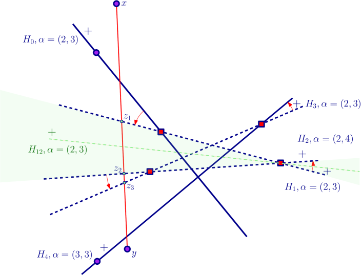
Figure 3: An example showing a sequence of rotations from $H_{0}$ to $H_{4}$ through $H_{1},H_{2},H_{3}$. Purple (disk) is the first color and red (square) is the second color. This sequence represents a path between two vertices in the UniqueEOPL graph that is generated in the reduction. The double-wedge is shaded and its angular bisector $H_{12}$ has the desired $\alpha$-vector.

This rotation function can be interpreted as a function that assigns each hyperplane to the next hyperplane. The set of colorful hyperplanes can be interpreted as vertices in a graph with the rotation function determining the connectivity of the graph.

Canonical path.

Each colorful hyperplane $H$ is incident to a colorful set of $d$ points. This set of points defines $d$ possible anchors, and each anchor can be used to rotate $H$ in a different fashion. To define a unique sequence of rotations, we pick a specific order as follows: first, we assume that the colorful hyperplane $H$ whose $\alpha$-vector is $(1,\ldots,1)$ is given (we show later how this assumption can be removed). We start at $H$ and pick the anchor that excludes the first color, then apply a sequence of rotations until we hit another colorful hyperplane with $\alpha$-vector $(2,1,\ldots,1)$. Similarly, we move to a colorful hyperplane with $\alpha$-vector $(3,1,\ldots,1)$ and so on until we reach $(\alpha_{1},1,\ldots,1)$. Then, we repeat this for the other colors in order to reach $(\alpha_{1},\alpha_{2},1,\ldots,1)$ and so on until we reach the target $\alpha$-vector. This pattern of $\alpha$-vectors helps in defining a potential function that strictly increases along the path. We can encode this sequence of rotations as a unique path in the UniqueEOPL instance, and we call it canonical path.

A natural way to define the UniqueEOPL graph would be to consider hyperplanes as the vertices in the graph. However, this leads to complications. Figure 3 shows a rotation from $H_{0}$ to $H_{4}$, with $\alpha$-vectors $(2,3)$ and $(3,3)$ respectively. During the rotation, we encounter a hyperplane $H_{2}$ for which its $\alpha$-vector is $(2,4)$, which differs from our desired sequence of $(2,3),\dots,(2,3),(3,3)$. This makes it difficult to define a potential function in the graph that strictly increases along the path $v_{H_{0}},\dots,v_{H_{4}}$ where $v_{H_{i}}$ is the vertex representing hyperplane $H_{i}$. One way to alleviate this problem is to not use $H_{i}$ as a vertex directly, but the double-wedge that is traced out by the rotation from $H_{i}$ to $H_{i+1}$. If the $\alpha$-vector is now measured using the hyperplane that bisects the double-wedge, then we get the desired sequence of $(2,3),\dots,(2,3),(3,3)$. See Figure 3 for an example.

With additional overhead, the rotation function can be extended to double-wedges. This in turn also leads to a neighborhood graph where the vertices are the double-wedges and the rotations can be used to define the edges. The graph is connected and has a grid-like structure that may be of independent interest. To simplify the exposition, we postpone the description of double-wedges and the associated graph to Section 4.

Distance parameter and potential function.

The $\alpha$-vector is not sufficient to define the potential function, since the sequence of rotations between two colorful hyperplanes may have the same $\alpha$-vector. For instance, the bisectors of the rotations in $H_{0},\dots,H_{3}$ in Figure 3 all have the same $\alpha$-vector. Hence, we need an additional measurement in order to determine the direction of rotation that increases the $\alpha$-vector.

Similar to how we define the orientation for a non-colorful hyperplane, let $H$ denote a hyperplane that passes through points of $(d-1)$ colors. Let $P_{j}$ denote the missing color in $H$. Let $x,y\in P_{j}$ be the highest ranked points under $\prec_{j}$ in $H^{+}$ and $H^{-}$ respectively. Let $z$ denote the intersection of $xy$ and $H$. We define a distance parameter called dist-value of $H$ to be the distance $\|x-z\|$. In Figure 3, we can see that rotating from $H_{0}$ to $H_{4}$ sweeps the segment $xy$ in one direction, with the dist-value of the hyperplanes increasing strictly. This is sufficient to break ties and hence determine the correct direction of rotation. The precise statement is given in Lemma 6. We can extend this definition to the domain of double-wedges. We define a potential value for each vertex on the canonical path in UniqueEOPL using the sum of weighed components of $\alpha$-vector and dist-value for the tie-breaker.

Correctness.

We show that if there are no violations, we can always apply Procedure $NextRotate$ to increment the $\alpha$-vector until we find the desired solution, which implies that the canonical path exists. If the input satisfies weak general position, we can see that the rotating hyperplane always hits a unique point in Step $5$, which may be swapped to form a new anchor in Step $7$.

The well-separation condition guarantees that the potential function always increases along the rotation. Let $H_{1},H_{2}$ denote a pair of hyperplanes that are the input and output of Procedure $NextRotate$ respectively. Let $H$ denote any intermediate hyperplane during the rotation from $H_{1}$ to $H_{2}$ through the common anchor. Let $P_{j}$ be the color missing from the anchor and $x$ be the highest ranked point under $\prec_{j}$ in $H_{1}^{+}$. We say that the orientation of $H_{2}$ (resp. $H$) is consistent with that of $H_{1}$ if $x\in H_{2}^{+}$ (resp. $x\in H^{+}$). Lemma 5 shows that the orientations are always consistent when $H_{1}$ and $H_{2}$ are non-colorful hyperplanes even without the assumption of well-separation.

Lemma 5 (consistency of orientation).

Assume that weak general position holds. Let $H_{1},H_{2}$ be the input and output of Procedure $NextRotate$ respectively. Let $H$ denote any intermediate hyperplane within the rotation. The orientations of $H_{1}$ (resp. $H_{2}$) and $H$ are consistent when $H_{1}$ (resp. $H_{2}$) is a non-colorful hyperplane.

Proof.

Since $H_{1}$ is a non-colorful hyperplane, let $P_{j}$ denote the color missing from $H_{1}$. $H_{1}$ and $H$ give the same partition of $P_{j}$ into two sets because the continuous rotation from $H_{1}$ to $H$ does not hit any point in $P_{j}$. Let $x$ and $y$ be the highest ranked points under $\prec_{j}$ in each set. Since we have weak general position, the segment $xy$ cannot pass through the anchor of the rotation so that the orientations of $H_{1}$ and $H$ are well-defined by the $(d-1)$ colored points in the anchor and the intersections of the hyperplanes with the segment $xy$. Thus, the determinant defining the normal of the rotating hyperplane from $H_{1}$ to $H$ for the orientation is always non-zero. Since the intersection of the rotating hyperplane from $H_{1}$ to $H$ and the segment $xy$ moves continuously along $xy$, by a continuity argument, the normal of the hyperplane does not flip during the rotation. Without loss of generality, assume that $x\in H_{1}^{+}$. This implies that $x$ is always in the positive half-space of $H$ and hence $H$ has a consistent orientation as $H_{1}$. The same proof holds for $H_{2}$. ∎

Next, we show that the dist-value is strictly increasing for all the intermediate hyperplanes in the sequence of rotations from one colorful hyperplane to another colorful hyperplane.

Lemma 6.

Assume that weak general position holds. Let $H_{0}$ be a colorful hyperplane and $H_{k}$ be the first colorful hyperplane obtained by a sequence of rotations by Procedure $NextRotate$. We denote $H_{1},\ldots,H_{k-1}$ be the non-colorful hyperplanes obtained from the above sequence of rotations. The dist-values of $H_{1},\ldots,H_{k-1}$ is strictly increasing.

Proof.

Let $P_{j}$ denote the color missing from $H_{1}$. Then, $H_{2},\ldots,H_{k-1}$ all miss the color $P_{j}$, otherwise $H_{k}$ is not the first colorful hyperplane obtained by the rotations. Therefore, each $H_{i}$ gives the same partition of $P_{j}$ into two sets for $i=1,\ldots,k-1$ because the continuous rotations from $H_{1}$ to $H_{k-1}$ does not hit any point in $P_{j}$. Let $x$ and $y$ be the highest ranked points under $\prec_{j}$ in each set. Without loss of generality, assume that $x\in H_{1}^{+}$. Since $H_{1},\ldots,H_{k-1}$ are non-colorful hyperplanes, by Lemma 5, the consistent of the orientation can carry from $H_{1}$ to $H_{2}$ and so on. Then we have $x\in H_{1}^{+},\dots,x\in H_{k-1}^{+}$ and $y\in H_{1}^{-},\dots,y\in H_{k-1}^{-}$. Let $z_{1}=xy\cap H_{1},\dots,z_{k-1}=xy\cap H_{k-1}$. According to Step $5$ of Procedure $NextRotate$, each rotation is performed by moving away from $x$ along the segment $xy$. Hence we have $\|x-z_{1}\|<\|x-z_{2}\|<\dots<\|x-z_{k-1}\|$. ∎

The last step for proving that the potential function always increases along the canonical path is to show that the $\alpha$-vector increases in some coordinate from one colorful hyperplane to another colorful hyperplane through Procedure $NextRotate$. This requires the assumption of well-separation. Lemma 7 shows that if the orientations of $H_{1},H_{2}$ and $H$ are inconsistent, then well-separation is violated. By the contrapositive, if well-separation is satisfied, then all hyperplanes in the rotation always give consistent orientations. Then, it implies that rotating from a colorful hyperplane $H_{0}$ to another colorful hyperplane $H_{k}$ through a sequence of non-colorful hyperplanes that miss color $P_{j}$, we have $H_{0}^{+}\cap P_{j}\subset H_{k}^{+}\cap P_{j}$ and $H_{k}$ contains one additional point in $P_{j}$ that is hit by the last rotation. Therefore, $\alpha_{j}$ is increased by $1$ and other $\alpha_{i}$s keep the same value because of the way we swap the point of repeated color with the one in the anchor and the direction of rotation.

Lemma 7.

Assume that weak general position holds. Let $H_{1},H_{2}$ be the input and output of Procedure $NextRotate$ respectively. Let $R$ denote the anchor of the rotation from $H_{1}$ to $H_{2}$, and $P_{j}$ denote the color missing from $R$. Let $H$ denote any intermediate hyperplane within the rotation. If the orientations of $H_{1}$ (resp. $H_{2}$) and $H$ are inconsistent, then $H_{1}$ (resp. $H_{2}$) is a colorful hyperplane and we can find a colorful set $R\cup\{x^{\prime}\}$ lying in a $(d-2)$-flat where $x^{\prime}\in\mathrm{conv}(P_{j})$, in $O(d^{3})$ arithmetic operations. The set $R\cup\{x^{\prime}\}$ witnesses the violation of well-separation.

Proof.

Since the orientations of $H_{1}$ and $H$ are inconsistent, $H_{1}$ must be a colorful hyperplane by Lemma 5. Therefore, the point in $H_{1}$ that is not in the anchor is in $P_{j}$, denoted by $p$.

Let $x$ and $y$ be the points defined in Lemma 5 such that $x,y\in P_{j}$, and $x$ and $y$ are on different sides of $H_{1}$ and $H$. The $(d-2)$-flat containing $R$ separates $H_{1}$ and $H$ into two $(d-1)$-dimensional half-subspaces each. Let $H^{+}_{1,R}$ and $H^{+}_{R}$ be the half-subspaces intersecting with $xy$ on $H_{1}$ and $H$ respectively, and let us denote the intersection points by $z_{p}$ and $z$, respectively. The opposite half-subspaces are denoted by $H^{-}_{1,R}$ and $H^{-}_{R}$, respectively. By definition of the orientation for non-colorful hyperplanes, the orientation of $H$ is defined by $R\cup\{z\}$. Although the orientation of $H_{1}$ is defined by $R\cup\{p\}$, if we consider the determinant defining the orientation using $R\cup\{z_{p}\}$, it gives an orientation consistent with that of $H$. Therefore, it must be that $p\in H^{-}_{1,R}$. Then, we can see that the line segment $pz_{p}$ intersects the $(d-2)$-flat of $R$. We can compute $z_{p}$ and also the intersection point $x^{\prime}$ of $pz_{p}$ and the $(d-2)$-flat of $R$ by solving systems of linear equations with $d$ equations and $d$ variables in $O(d^{3})$ arithmetic operations. Since $x^{\prime}\in\mathrm{conv}(P_{j})$, $R\cup\{x^{\prime}\}$ is a colorful set contained in the $(d-2)$-flat of $R$. ∎

In order to guarantee that there is no other path in UniqueEOPL apart from the canonical path, we introduce self-loops for vertices that are not on the canonical path. The detailed proof is given in Lemma 17 that if there are no violations, then the reduced instance of UniqueEOPL only gives a (U1) solution, which readily translates to a (G1) solution, so our reduction is promise-preserving, and this can be done in polynomial time.

Since we do not know the hyperplane with $\alpha$-vector $(1,\dots,1)$ in advance, we split the problem into two sub-problems: in the first we start with any colorful hyperplane. We reverse the direction of the canonical path determined by the potential and construct an Alpha-HS instance for which the vertex with $\alpha$-vector $(1,\dots,1)$ is the solution. In the second, we use this vertex as the input to the main Alpha-HS instance. If the input is free of violations, then both sub-problems give valid solutions and together they answer the original question.

Handling violations.

The reduction maps violations of Alpha-HS to those of the UniqueEOPL instance, and certificates for the violations can be recovered from additional processing. When a violation of weak general position is witnessed on a vertex that lies on the canonical path, a hyperplane incident to $d$ colors may contain additional points. This in turn implies that some $\alpha$-cut is missing, so that the correct solution for the target may not exist. In addition, the (highest-ranked) points $x,y$ from the missing color that we choose to define the orientation of a non-colorful hyperplane may form a segment $xy$ that passes through the $(d-2)$-flat spanned by the anchor. In that case the orientation of the hyperplane is not well-defined. In the reduction, these problematic vertices are removed from the canonical path, thereby creating some additional starting points and end points in the reduced instance. These violations can be captured by (U1) with a wrong $\alpha$-vector or (UV2). Furthermore, the hyperplanes that contains the degenerate point sets could be represented by different choices of anchors and a additional point on the plane. Each such pair represents a vertex in the reduced instance. We join these vertices in the form of a cycle in the UniqueEOPL instance with all vertices having the same potential value, so that the violations can also be captured by (UV1) and (UV3).

When a violation of well-separation is witnessed on a vertex on the canonical path, the orientations of the two hyperplanes paired by Procedure $NextRotate$ may be inconsistent, which may not guarantee that the $\alpha$-vector is incremented in one component by one (See Figure 4). Hence, the canonical path is split into two paths that can be captured by (UV2). Furthermore, a violation of well-separation also creates multiple colorful hyperplanes with the same $\alpha$-vector (See Figure 4, left). Two vertices in the UniqueEOPL graph with the same potential value, which could correspond to some colorful or non-colorful hyperplanes, can be reported by (UV3). We show that this gives a certificate of violation of well-separation in the following lemmata, where $m_{0}$ is the number of bits used to represent each coordinate of points of $P$.

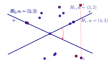
Figure 4: The examples show two sets of points that are not well-separated. Purple (circle) represents the first color and red (square) represents the second color. In both examples the rotation procedure does not increase the $\alpha$-vector. Both examples show that the orientation of the hyperplane may be flipped after the rotation, so the resulting $\alpha$-vector can go wrong.

Lemma 8.

Given two colorful hyperplanes $H_{p}$, $H_{q}$ with the same $\alpha$-vector, we can find a colorful set $\{x_{1}\in\mathrm{conv}(P_{1}),\ldots,x_{d}\in\mathrm{conv}(P_{d})\}$ that lies on a $(d-2)$-flat in $\mathrm{poly}(n,d,m_{0})$ time.

Proof.

Let $p_{1}\in P_{1},\ldots,p_{d}\in P_{d}$ denote the colorful points on $H_{p}$ and $q_{1}\in P_{1},\ldots,q_{d}\in P_{d}$ denote the colorful points on $H_{q}$. Throughout this proof, we consider $H^{+}$ to be a closed halfspace while $H^{-}$ is an open halfspace. We prove the claim by induction on the dimension $d$.

For the base case $d=2$, we have three different cases to consider depending on which cells out of $H_{p}^{-}\cap H_{q}^{+},H_{p}^{+}\cap H_{q}^{+},H_{p}^{+}\cap H_{q}^{-},H_{p}^{-}\cap H_{q}^{-}$ contain the segments $p_{1}q_{1}$ and $p_{2}q_{2}$. If the open segments $p_{1}q_{1}$ and $p_{2}q_{2}$ lie in either $H_{p}^{+}\cap H_{q}^{+}$ or $H_{p}^{-}\cap H_{q}^{-}$, then we can apply the same argument as in Lemma 19 to find a point $y$ that lies in $\mathrm{conv}(P_{1})\cap\mathrm{conv}(P_{2})$. In particular, $y$ could be the intersection point of $p_{1}q_{1}$ and $p_{2}q_{2}$ (see Figure 11(a)).

Without loss of generality, suppose that the open segment $p_{1}q_{1}\in H_{p}^{-}\cap H_{q}^{+}$. Since $p_{1}\in H_{p}^{+}\cap H_{q}^{+}$ and $q_{1}\in H_{p}^{-}\cap H_{q}^{+}$, there exists at least one point $r_{1}\in P_{1}\cap(H_{p}^{+}\cap H_{q}^{-})$ in order for $|P_{1}\cap H_{p}^{+}|=|P_{1}\cap H_{q}^{+}|$ to hold. If the open segment $p_{2}q_{2}$ also lies in $H_{p}^{-}\cap H_{q}^{+}$ (resp. $H_{p}^{+}\cap H_{q}^{-}$), then there exists at least one point $r_{2}$ in $P_{2}\cap(H_{p}^{+}\cap H_{q}^{-})$ (resp. $P_{2}\cap(H_{p}^{-}\cap H_{q}^{+})$). We can see that the intersection point $x$ of $H_{p}$ and $H_{q}$ lies inside the triangles $\triangle p_{1}q_{1}r_{1}$ and $\triangle p_{2}q_{2}r_{2}$ (see Figure 11(b)).

Suppose that the open segment $p_{2}q_{2}$ lies in $H_{p}^{+}\cap H_{q}^{+}$ (resp. $H_{p}^{-}\cap H_{q}^{-}$). In order to assign correct orientations to $H_{p}$ and $H_{q}$, the order in which points of $P_{1}$ and $P_{2}$ appears on the hyperplanes along any direction must be the same for both. This is only feasible when $p_{2}$ lies between $p_{1}$ (resp. $q_{1}$) and the intersection point $x=H_{p}\cap H_{q}$. Hence, $p_{2}$ (resp. $q_{2}$) lies inside the triangles $\triangle p_{1}q_{1}r_{1}$ (see Figure 11(c)).

For $d>2$, if $H_{p}\cap H_{q}$ does not intersect $\mathrm{conv}(P_{i})$ for all $i\in[d]$, then the claim follows from Lemma 19. Without loss of generality, suppose that $H_{p}\cap H_{q}$ intersects $\mathrm{conv}(P_{1})$. We can use linear programming to check whether there is a hyperplane $H$ that separates $P_{1}$ and $\cup_{i\in[2..d]}P_{i}$. If $H$ does not exist, by Lemma 1, we can find a desired colorful set and we are done. Otherwise, we use linear programming to find a point $x_{1}\in H_{p}\cap H_{q}\cap\mathrm{conv}(P_{1})$. Then, we project $\cup_{i\in[2..d]}P_{i}$ towards $x_{1}$ onto $H$. Let $P_{i}^{\prime}$ be the projected point set for $i\in[2..d]$. Let $H_{p}^{\prime}$ and $H_{q}^{\prime}$ be $H_{p}\cap H$ and $H_{q}\cap H$, respectively. From the way we do the projection, $H_{p}^{\prime}$ and $H_{q}^{\prime}$ keep the same $\alpha$-vector with respect to $P_{i}^{\prime}$ on the hyperplane $H$. By induction, we can find a colorful set $\{x_{2}^{\prime}\in\mathrm{conv}(P_{2}^{\prime}),\ldots,x_{d}^{\prime}\in\mathrm{conv}(P_{d}^{\prime})\}$ that lies on a $(d-3)$-flat. Then, we shoot a ray from $x_{1}$ towards $x_{i}^{\prime}$ until it hits some point $x_{i}\in\mathrm{conv}(P_{i})$ and we can see that $\{x_{1},x_{2},\ldots,x_{d}\}$ spans a $(d-2)$-flat. ∎

Lemma 9.

Given two non-colorful hyperplanes that each contains $d-1$ points and have the same missing color, $\alpha$-vector and dist-value, we can find a colorful set of points $\{x_{1}\in\mathrm{conv}(P_{1}),\ldots,x_{d}\in\mathrm{conv}(P_{d})\}$ that lies on a $(d-2)$-flat in $\mathrm{poly}(n,d,m_{0})$ time.

Proof.

The idea is to transform $P$ to a point set $P^{\prime}$, in which we can find two points from the missing color that can each be moved onto one of the non-colorful hyperplanes. Then, the two non-colorful hyperplanes become colorful hyperplanes in $P^{\prime}$ with the same $\alpha$-vector so that we are in the setup of Lemma 8 and the claim follows.

Without loss of generality, we assume that the missing color of the two non-colorful hyperplanes is color 1. Let $H_{p}$ denote one of the non-colorful hyperplanes that passes through some $p_{2}\in P_{2},\ldots,p_{d}\in P_{d}$ and $H_{q}$ denote another non-colorful hyperplane that passes through some $q_{2}\in P_{2},\ldots,q_{d}\in P_{d}$. Recall that they have the same $\alpha$-vector and dist-value. Let $x_{p},y_{p}$ (resp. $x_{q},y_{q}$) be the highest ranked points of $P_{1}$ under $\prec_{1}$ on either side of $H_{p}$ (resp. $H_{q}$) and let $z_{p}$ (resp. $z_{q}$) be the intersection of segment $x_{p}y_{p}$ (resp. $x_{q}y_{q}$) with $H_{p}$ (resp. $H_{q}$). By the definition and assumption of dist-value, the dist-value of $H_{p}$ and $H_{q}$ is $||x_{p}-z_{p}||=||x_{q}-z_{q}||$.

Throughout this proof, we consider $H^{+}$ to be a closed halfspace while $H^{-}$ is an open halfspace. Our definition of $P^{\prime}$ changes depending on the locations of $x_{p},x_{q},y_{p},y_{q}$ in the cells $H_{p}^{-}\cap H_{q}^{+},H_{p}^{+}\cap H_{q}^{+},H_{p}^{+}\cap H_{q}^{-},H_{p}^{-}\cap H_{q}^{-}$. When $x_{p},x_{q}\in H_{p}^{+}\cap H_{q}^{+}$ and $y_{p},y_{q}\in H_{p}^{-}\cap H_{q}^{-}$, we have $x_{p}=y_{q}$ and $y_{p}=y_{q}$. Since $||x_{p}-z_{p}||=||x_{q}-z_{q}||$, we also have $z_{p}=z_{q}$, which implies that $H_{p}\cap H_{q}$ intersects $\mathrm{conv}(P_{1})$. Similar to the proof of Lemma 8, we find a separating hyperplane $H$ between $P_{1}$ and $\cup_{i\in[2..d]}P_{i}$ if it exists. Then, we project $\cup_{i\in[2..d]}P_{i}$ towards $z_{p}$ onto $H$, in which we have two colorful hyperplanes with the same $\alpha$-vector in $\mathbb{R}^{d-1}$, so we can apply Lemma 8 to the sub-problem in $\mathbb{R}^{d-1}$ and recover a desired colorful set as in Lemma 8. If $H$ does not exist, by Lemma 1 we can also find a desired colorful set and we are done.

In the following, we consider the case of $x_{p},x_{q}\in H_{p}^{+}\cap H_{q}^{+}$ with three sub-cases:

• $[y_{p}\in H_{p}^{-}\cap H_{q}^{+}\mbox{ and }y_{q}\in H_{p}^{-}\cap H_{q}^{-}]$: there must exist a point $r\in P_{1}(\cap H_{p}^{+}\cap H_{q}^{-})$, otherwise $H_{p}$ and $H_{q}$ cannot have the same $\alpha$-vector. Then, we move $y_{p}$ towards $x_{p}$ along segment $x_{p}y_{p}$ until it hits $H_{p}$ at $z_{p}$. Similarly, we move $r$ towards $x_{p}$ along segment $x_{p}r$ until it hits $H_{q}$. We define the resulting point set to be $P^{\prime}$. We can see that both of the first coordinates of the $\alpha$-vectors of $H_{p}$ and $H_{q}$ (with respect to $P^{\prime}$) are increased by 1, so they still have the same $\alpha$-vector, and now $H_{p}$ and $H_{q}$ are colorful hyperplanes in $P^{\prime}$. By Lemma 8, we can find a colorful set $\{x_{1}\in\mathrm{conv}(P_{1}^{\prime}),\ldots,x_{d}\in\mathrm{conv}(P_{d}^{\prime})\}$ that lies on a $(d-2)$-flat. Since $y_{p}$ and $r$ only moved inside $\mathrm{conv}(P_{1})$, $\mathrm{conv}(P^{\prime}_{1})\subseteq\mathrm{conv}(P_{1})$ and $P^{\prime}_{i}=P_{i}$ for $i=[2..d]$. Since the colorful set is also a certificate for $P$, we are done.

• $[y_{p}\in H_{p}^{-}\cap H_{q}^{-}\mbox{ and }y_{q}\in H_{p}^{+}\cap H_{q}^{-}]$: the argument is symmetrical to the case above.

• $[y_{p}\in H_{p}^{-}\cap H_{q}^{+}\mbox{ and }y_{q}\in H_{p}^{+}\cap H_{q}^{-}]$: we move $y_{p}$ towards $x_{p}$ along segment $x_{p}y_{p}$ until it hits $H_{p}$ and move $y_{q}$ towards $x_{q}$ along segment $x_{q}y_{q}$ until it hits $H_{q}$.

Next, we consider $x_{p}\in H_{p}^{+}\cap H_{q}^{+}$ and $x_{q}\in H_{p}^{-}\cap H_{q}^{+}$.

• $[y_{p}\in H_{p}^{-}\cap H_{q}^{+}\mbox{ and }y_{q}\in H_{p}^{-}\cap H_{q}^{-}]$: we have $x_{q}=y_{p}$. We move $x_{p}$ towards $x_{q}$ along segment $x_{p}x_{q}$ until it hits $H_{p}$ and move $x_{q}$ towards $y_{q}$ along segment $x_{q}y_{q}$ until it hits $H_{q}$.

• $[y_{p}\in H_{p}^{-}\cap H_{p}^{-}\mbox{ and }y_{q}\in H_{p}^{+}\cap H_{q}^{-}]$: we move $x_{p}$ towards $x_{q}$ along segment $x_{p}x_{q}$ until it hits $H_{p}$ and move $x_{q}$ towards $y_{p}$ along segment $x_{q}y_{p}$ until it hits $H_{q}$.

• $[y_{p}\in H_{p}^{-}\cap H_{q}^{+}\mbox{ and }y_{q}\in H_{p}^{+}\cap H_{q}^{-}]$: we have $x_{q}=y_{p}$. We move $y_{p}$ towards $x_{p}$ along segment $x_{p}y_{p}$ until it hits $H_{p}$ and move $y_{q}$ towards $x_{p}$ along segment $x_{p}y_{q}$ until it hits $H_{q}$.

• $[y_{p}\in H_{p}^{-}\cap H_{q}^{-}\mbox{ and }y_{q}\in H_{p}^{-}\cap H_{q}^{-}]$: we have $y_{p}=y_{q}$. We move $x_{p}$ towards $x_{q}$ along segment $x_{p}x_{q}$ until it hits $H_{p}$ and move $x_{q}$ towards $y_{q}$ along segment $x_{q}y_{q}$ until it hits $H_{q}$.

The case for $x_{p}\in H_{p}^{+}\cap H_{q}^{-}$ and $x_{q}\in H_{p}^{+}\cap H_{q}^{+}$ are symmetrical to those above.

The last case is $x_{p}\in H_{p}^{+}\cap H_{q}^{-}$ and $x_{q}\in H_{p}^{-}\cap H_{q}^{+}$. Basically, the sub-cases are the same as those above except one, which happens for $y_{p}\in H_{p}^{-}\cap H_{p}^{+}$ and $y_{q}\in H_{p}^{+}\cap H_{q}^{-}$. In this case, we have $x_{p}=y_{q}$ and $x_{q}=y_{p}$. We move $x_{p}$ and $x_{q}$ towards each other along segment $x_{p}x_{q}$ and until they hit $H_{p}$ and $H_{q}$. Note that the segment $x_{p}x_{q}$ may intersect the $(d-2)$-flat $H_{p}\cap H_{q}$, but this case is also handled by Lemma 8. ∎

For the second output ($\mathbb{V}(v)<\mathbb{V}(u)<\mathbb{V}(\mathbb{S}(v))$) of (UV3), there are two cases to consider. In the first case, if both $v$ and $\mathbb{S}(v)$ correspond to the same $\alpha$-vector, then $u$ also has the same $\alpha$-vector and its dist-value is between that of $v$ and $\mathbb{S}(v)$. Since rotating the hyperplane from $v$ to $\mathbb{S}(v)$ does not pass through $u$, we can find a different hyperplane that is interpolated by $v$ and $\mathbb{S}(v)$ and has the same dist-value as $u$. Hence, we apply Lemma 9 again to find a witness of the violation. For the second case that the $\alpha$-vector of $\mathbb{S}(v)$ increases in one coordinate by one from that of $v$, since the role of dist-value is dominated by the role of $\alpha$-vector in the potential function, the dist-value of $u$ can be arbitrarily large. Therefore, we may not be able to apply the interpolation technique from the first again. We argue that we can transform $P$ to a point set $P^{\prime}$ satisfying $\mathrm{conv}(P^{\prime}_{i})\subseteq\mathrm{conv}(P_{i})$ for all $i\in[d]$, such that the hyperplanes of $v$ and $u$ become colorful. Then, we apply Lemma 8 to show that $P^{\prime}$ is not well-separated, which also implies that $P$ is not well-separated. The precise statement and proof are given in Lemma 21.

In Lemma 23 we show how to compute a (GV1) solution from a (UV1) solution. In Lemmas 24 and 25 we show how we can compute a (GV1) or (GV2) solution, given a (UV2) or (UV3) solution. A (GV1) or (GV2) solution can also occur with a (U1) solution that has the incorrect $\alpha$-vector, and we show how to do this in Lemma 22. We show that converting these solutions always takes $\mathrm{poly}(n,d)$ time. The violations may be detected in either the first sub-problem or the second sub-problem. Our constructions thus culminate in the promised result:

Theorem 10.

Alpha-HS $\in$ $\mathsf{UEOPL}$ $\subseteq$ $\mathsf{CLS}$.

4 Double-wedges and the neighborhood graph

In this section we formally define the notion of double-wedges and the underlying graph that is defined using rotations.

4.1 Double-wedges

An anchor is a colorful $(d-1)$-tuple of $P$ which spans a $(d-2)$-flat. Let $P_{i}$ denote the missing color in the anchor. Then the tuple for the anchor $R=(p_{1},\dots,p_{d-1})$ is ordered as $R=\{p_{1}\in P_{1},\dots,p_{i-1}\in P_{i-1},p_{i}\in P_{i+1},\dots,p_{d-1}\in P_{d}\}$. An anchor $R$ along with a pair of points $p,q\in P$ such that $p,q\not\in R$ is called a double-wedge if all of the following hold:

• the hyperplane $H_{p}$ through $R\cup\{p\}$ does not contain $q$. This implies that the hyperplane $H_{q}$ through $R\cup\{q\}$ does not contain $p$.

• if $x,y$ are the highest ordered points of $P_{i}$ under $\prec_{i}$ on either sides of $H_{p},H_{q}$, then $R\cup\{x,y\}$ does not lie on a hyperplane.

• the hyperplanes $H_{p}$ and $H_{q}$ both intersect each of the convex hulls $\mathrm{conv}(P_{1}),\dots,\mathrm{conv}(P_{d})$. If a hyperplane is colorful, the orientation is defined naturally. Suppose $H_{q}$ is non-colorful, then we have $(d-1)$ colors in $R\cup\{q\}$, so we use $R$ and a point in the convex hull of the missing color to define the orientation as described previously.

• the intersection of the open halfspaces $H_{q}^{+}\cap H_{p}^{-}$ is empty, that is, it does not contain any point of $P$. Similarly $H_{p}^{+}\cap H_{q}^{-}$ must also be empty.

We visualize the anchor as a $(d-2)$-ridge through which $H_{p},H_{q}$ pass through. A rotation around the anchor changes one hyperplane to the other without passing through any other point of $P$. Intuitively the double-wedge refers to the space $(H_{q}^{+}\cap H_{p}^{-})\cup(H_{p}^{+}\cap H_{q}^{-})$ and we use this interpretation several times. See Figure 5 for a simple example.

Figure 5: A double-wedge $(R,p,q)$ with indicated orientations. The shaded region is empty.

For a double-wedge $w:=(R,p,q)$, we define a representative hyperplane $H_{w}$ as the hyperplane that is the angular bisector of the double-wedge. Since a double-wedge is empty, $H_{w}$ does not contain any point of $P$ apart from $R$. We define an orientation for $H_{w}$ based on $R$ and the color missing from $R$. Let $x,y$ be points from the missing color as defined before. Without loss of generality, let $x\in H_{w}^{+}$, and $y\in H_{w}^{-}$. We call the first hyperplane among $H_{p},H_{q}$ that intersects the directed segment $xy$ as the upper hyperplane of $w$ and the other hyperplane as the lower hyperplane of $w$. A simple example can be found in Figure 6.

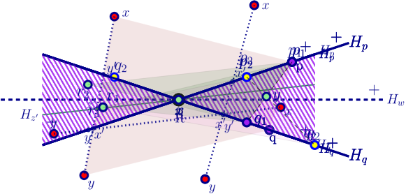
Figure 6: The points $x,y$ are from the missing color.

The $\alpha$-vector of any oriented hyperplane $H$ is a $d$-tuple $(a_{1},\dots,a_{d})$ of integers where $a_{i}$ is the number of points of $P_{i}$ in the closed halfspace $H^{+}$ for $i\in[d]$. The $\alpha$-vector of a double-wedge $w=(R,p,q)$ is defined as the $\alpha$-vector of its representative hyperplane. We say that a double-wedge $w=(R,p,q)$ is non-colorful, if both $R\cup\{p\}$ and $R\cup\{q\}$ are non-colorful, and colorful, if exactly one of $R\cup\{p\}$ and $R\cup\{q\}$ is colorful, and very colorful, if both $R\cup\{p\}$ and $R\cup\{q\}$ are colorful.

Under the assumption of weak general position, we additionally have that if $w$ is non-colorful, then $H_{p},H_{q}$ are non-colorful, and if $w$ is colorful, exactly one of $H_{p},H_{q}$ is colorful, and if $w$ is very colorful, both $H_{p},H_{q}$ are colorful.

Remark 11.

The definition of dist-value for hyperplanes can be extended to double-wedges by setting the dist-value of a double-wedge as that of its representative hyperplane. Consequently, the results of Lemmas 5, 6 and 7 extend to double-wedges with simple modifications.

4.2 Defining a neighborhood graph

We define a concept of neighborhood between double-wedges, and then we use this to define a graph whose vertices correspond to the double-wedges. We first describe the graph under the assumptions that the colors are well-separated and $P$ is in weak general position. Later we show how to handle the cases when these assumptions fail.

We call two double-wedges $(R,p,q),(R^{\prime},p^{\prime},q^{\prime})$ neighboring if both share a common hyperplane, that is, $\{H_{p},H_{q}\}\cap\{H_{p^{\prime}},H_{q^{\prime}}\}\neq\varnothing$, with an exception that we elaborate below. A double-wedge $w=(R,p,q)$ has different number of neighbors depending on how colorful its hyperplanes are. The anchor can be written in the form $R=\{x_{1},\dots,x_{d-1}\}$.

1. Let $w$ be non-colorful. Then $p,q$ both share their colors with those of $R$. Suppose $p$ has the same color as $x_{i}$. Then there are at most three neighboring double-wedges that share $H_{p}$. One of them use the same anchor $R$, and as an exception we do not count this as a neighboring double-wedge. For the two remaining neighbors, the anchor is $R^{\prime}=(x_{1},\dots,p,\dots,x_{d-1})$ where $p$ has replaced $x_{i}$. The two rotational directions determine the two double-wedges. Only one of them has the same $\alpha$-vector as $w$, since the representative hyperplanes contain $x_{i}$ on opposite sides. With a similar argument, there are at most two neighboring double-wedges that share $H_{q}$ and at most one of them has the same $\alpha$-vector as $w$.

2. Let $w$ be colorful, where $H_{p}$ is colorful and $H_{q}$ is non-colorful, without loss of generality. By replacing some $x_{i}$ by $p$ we get an anchor that is contained in $H_{p}$ and which may define a double-wedge for each of the two rotational directions. Since there are $(d-1)$ possible anchors formed by replacement, there are at most $2(d-1)$ double-wedges that share $H_{p}$. Additionally, keeping the anchor $R$ fixed, there is at most one neighboring double-wedge. So there are at most $2d-1$ neighboring double-wedges of $w$ that share $H_{p}$. The case for $H_{q}$ is similar to case (1).

3. Let $w$ be very colorful. Similar to case (2), there are at most $2d-1$ double-wedges sharing $H_{p}$. The case for $H_{q}$ is similar.

The neighborhood graph.

We build a graph $G$ where each vertex corresponds to a double-wedge. Let $w=(R,p,q)$ be any double-wedge. For simplicity, we denote the vertex in $G$ corresponding to $w$ also by $w$. If $H_{p}$ is colorful, we add an edge in $G$ between $w$ and the vertex of each neighboring double-wedge that shares $H_{p}$. If $H_{p}$ is non-colorful, we add an edge only with the vertex of the double-wedge that shares its $\alpha$-vector with that of $w$. Thus, non-colorful double-wedges have degree two in $G$, while colorful and very colorful double-wedges have degrees at most $2d$ and $4d-2$, respectively.

We transfer each attribute of a double-wedge to its vertex in $G$. For instance, we call vertices of $G$ as non-colorful, colorful or very colorful corresponding to the color of the double-wedge representing the vertex. Similarly, each vertex has an $\alpha$-vector that corresponds to the $\alpha$-vector of its double-wedge, and so on. See Figure 7 for an elementary example.

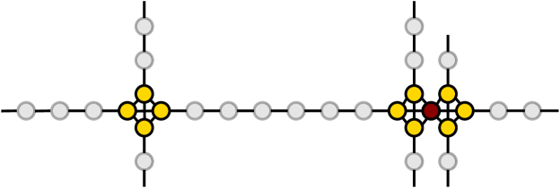
Figure 7: A subgraph of $G$: the gray vertices (lightly shaded) are non-colorful, the golden vertices (shaded) are colorful, and the red vertices (heavily shaded) are very colorful.

Let $v\in G$ be any vertex and let $(\alpha_{1},\dots,\alpha_{d})$ denote the $\alpha$-vector of $v$. The largest $\alpha$-vector for any hyperplane is $(n_{1},\dots,n_{d})$ that occurs on a unique tangent hyperplane whose half-space contains $P$. With our definition of the $\alpha$-vector of double-wedges using the representative hyperplanes, for any double-wedge $w$, the $\alpha$-vector of $w$ is smaller in at least one coordinate from the maximum.

Lemma 12 (Grid-like structure).

Let $H$ be a colorful hyperplane with $\alpha$-vector $(\alpha_{1},\dots,\alpha_{d})$. For each $j\in[d]$, if $\alpha_{j}\leq n_{j}-1$ (resp. $\alpha_{j}\geq 2$), then there is a path $w,w_{1},w_{2},\dots,w_{k},w^{\prime}$ in $G$ such that the double-wedge $w$ is incident to $H$, the double-wedge $w^{\prime}$ is incident to another colorful hyperplane $H^{\prime}$, $w,w_{1},w_{2},\dots,w_{k}$ share the same $\alpha$-vector and the $\alpha$-vector for $H^{\prime}$ differs only in the $j$-th component, where the value is $\alpha_{j}+1$ (resp. $\alpha_{j}-1$).

Proof.

For the case that $\alpha_{j}\leq n_{j}-1$, we set an anchor $R$ in $H$ that excludes the $j$-th colored point, say $p_{j}$. Then, we apply Procedure $NextRotate$ starting from $(R,p_{j})$ until we get another colorful hyperplane $H^{\prime}$. Let $w$ be the double-wedge created by the first rotation. Note that $p_{j}$ is on the upper hyperplane of $w$. During this sequence of rotations, we also get a sequence of double-wedges. Before the rotating hyperplane $H^{\prime\prime}$ hits a point $p_{i}$ of repeated color $i$, assume that $p_{i}$ is in the negative half-space of $H^{\prime\prime}$. Once $p_{i}$ is on $H^{\prime\prime}$, we swap $p_{i}$ with another point $p^{\prime}_{i}$ of the same color in the anchor and keep the rotation towards the opposite direction of the orientation so that $p_{i}$ is in the positive half-space of $H^{\prime\prime}$ and $p^{\prime}_{i}$ from the positive half-space moves to the negative half-space. This is true because the orientation is consistent by Lemma 5. If $p_{i}$ is in the positive half-space of $H^{\prime\prime}$ before $p_{i}$ is hit by $H^{\prime\prime}$, then $p_{i}$ remains in the positive half-space and $p^{\prime}_{i}$ as well (see Figure 3). Both cases maintain $\alpha_{i}$ during the rotation. Thus, all non-colorful double-wedges in this sequence of rotations have the same $\alpha$-vector as $w$. In the last rotation, the rotating hyperplane hits the first point $p^{\prime}_{j}$ of color $j$. By Lemma 7, well-separation guarantees the consistency of the orientation of the rotating hyperplane so that $p^{\prime}_{j}$ moves from the negative half-space to the positive half-space and other points of color $j$ remain in the same sides of the hyperplane. Thus, $\alpha_{j}$ is increased by one. The same argument also works for the case that $\alpha_{j}\geq 2$ by using the inverse of Procedure $NextRotate$.

Since all the double-wedges created by the first rotation for each $j$ are incident to $H$, they are also connected in $G$ by definition. ∎

By making use of Lemma 12, we show that:

Lemma 13.

The neighborhood graph $G$ is connected.

Proof.

By Lemma 12, we know that all (very) colorful double-wedges are connected. For non-colorful double-wedges, we apply Procedure $NextRotate$ on its lower hyperplane until the rotating hyperplane hits some point of the missing color, which implies that non-colorful double-wedges also connect to some (very) colorful double-wedge. ∎

The neighborhood graph $G$ imitates a grid in a coarse sense. There is a ”vertex” for every colorful $d$-tuple of $P$, and there are paths connecting these grid vertices. We showed in Lemma 13 that $G$ is connected. Therefore, given a target $\alpha$-vector $(\alpha_{1},\dots,\alpha_{d})$, the correct $d$-tuple can be found by starting from some vertex and walking towards the solution. See Figure 8 for an illustration.

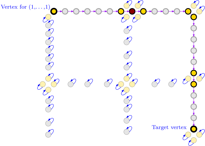
Figure 8: The canonical path is marked with arrows. All other vertices in the graph have self-loops.

If $P$ violates well-separation or weak general position, then many nice properties of the neighborhood graph are destroyed. Double-wedges may fail to have consistent orientations by Lemma 7. There may be multiple solutions for the same $\alpha$-cut, and no solutions for other cuts. The former case will manifest as multiple vertices with the same $\alpha$-vector, but they may lie in different connected components, so Lemma 13 will fail, making the graph disconnected. For the latter case, there will be no vertex in $G$ that corresponds to the $\alpha$-cut. The grid-like structure exhibited in Lemma 12 is also not applicable anymore, meaning that the canonical path may not exist. See Figure 9 for a graph that contains violations.

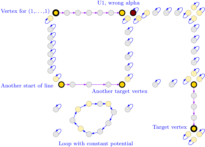
Figure 9: A subgraph with multiple violations.

5 The formal reduction

In this section, we give a formal reduction from an instance $\cal{I}$ of Alpha-HS to an instance $\cal{I^{\prime}}$ of UniqueEOPL in polynomial time. An instance $\cal{I}$ of Alpha-HS is defined by $d$ finite sets of points $P=P_{1}\cup\ldots\cup P_{d}$ in $\mathbb{R}^{d}$ and a vector $(\alpha_{1},\ldots,\alpha_{d})$ of positive integers that satisfy $a_{i}\leq|P_{i}|$ for $i=1,\dots,d$. Let $m_{0}$ be the number of bits needed to represent each coordinate of points in $P$ and let $n_{0}$ denote $\max_{i\in[d]}|P_{i}|$. Let $k$ denote the number of coordinates of $\alpha$ that are not equal to one. Without loss of generality, we assume that $\{\alpha_{1},\dots,\alpha_{k}\}$ are the non-unit entries in $\alpha$. Suppose that $(\alpha_{1},\ldots,\alpha_{d})\neq(1,\ldots,1)$ and we are also given a transversal hyperplane $H_{0}$ passing through some $p^{\prime}_{1}\in P_{1},\ldots,p^{\prime}_{d}\in P_{d}$ with $\alpha$-vector $=(1,\ldots,1)$. Later, we show that we do not need to know $H_{0}$ in advance. Then, we construct an UniqueEOPL instance $\cal I^{\prime}$ on vertex set $\{0,1\}^{\kappa}$, where $\kappa=3\cdot\lceil\log d\rceil+(d+1)\cdot\lceil\log n_{0}\rceil$ and with procedures $\mathbb{S}$, $\mathbb{P}$ and $\mathbb{V}$ , where $\mathbb{V}:\{0,1\}^{k}\rightarrow\{0,\ldots,2^{\gamma}-1\}$ and $\gamma=O(\mathrm{poly}(d,n_{0},m_{0}))$.

As shown in Section 3, a vertex $v$ in $\cal I^{\prime}$ corresponds to $(R,p,q)$ in $\cal I$, where $R$ is a colorful point set of size $(d-1)$ from $P$, and $p,q\in P$. We are only interested in the case when $(R,p,q)$ is a double-wedge, as per the definition in Section 4.1. Otherwise, we create a self loop on $v$ in $\cal{I^{\prime}}$. Furthermore, if there are no violations in $\cal I$, we can define a canonical path from the vertex $v_{0}$ with $\alpha$-vector $=(1,\ldots,1)$ to the unique vertex $v_{\alpha}$ with $\alpha$-vector $=(\alpha_{1},\dots,\alpha_{d})$ (shown in Section 3.1), which is the unique path in $\cal I^{\prime}$. For other vertices $v$ not on the path, we also create a self loop on $v$. For instance, when $\cal I$ fails weak general position assumption, then $R\cup\{p_{1},p_{2},\ldots,p_{m}\}$ lie on the same hyperplane, where $p_{1}\prec\dots\prec p_{m}\in P$. In this case we create a cycle on $v_{1}=(R,p_{1},q),v_{2}=(R,p_{2},q),\ldots,v_{m}=(R,p_{m},q)$ with the same potential value on each $v_{i}$, so that this violation may be reported as the violation (UV1) in $\cal I^{\prime}$. When $\cal I$ fails the well-separated assumption, the graph we constructed may contain more than one path, which may be reported as the violations (UV2) or (UV3) in $\cal I^{\prime}$. In particular, if a hyperplane witnesses both the violations of weak general position and well-separation, then the cycle may become a path with the same potential value, so any violation could be possible.

First we describe how to represent a tuple $(R,p,q)$ in $\kappa$ bits. Each vertex is represented as a $(d+4)$-tuple $(t_{1},\ldots,t_{d+4})\in\mathbb{Z}^{d+4}$ such that

• $t_{1}$ contains $\lceil\log d\rceil$ bits representing the index of the missing color in $R$,

• $t_{2},\ldots,t_{d}$ each contain $\lceil\log n_{0}\rceil$ bits for the indices of the points in $R$ ordered by $\prec$,

• $(t_{d+1},t_{d+2})$ contain $\lceil\log d\rceil$ and $\lceil\log n_{0}\rceil$ bits for the index of the color and the index of $p\in P_{t_{d+1}}$ respectively,

and we use the same idea to represent $q$ by $(t_{d+3},t_{d+4})$. Altogether, we need at most $\kappa=3\cdot\lceil\log d\rceil+(d+1)\cdot\lceil\log n_{0}\rceil$ bits in the encoding. Let $f_{v}:\{P\}^{d+1}\rightarrow\{0,1\}^{\kappa}$ denote the function that encodes $(R,p,q)$ to $(t_{1},\ldots,t_{d+4})$. If $(R,p,q)$ is a double-wedge, then $(R,q,p)$ also represents the same double-wedge. Since we do not want to create two valid vertices in $G$ corresponding to the same double-wedge, we only pick the one with $(t_{d+1},t_{d+2})$ on the upper hyperplane as a valid double-wedge. The following lemma details how we can verify whether a given encoding $(t_{1},\ldots,t_{d+4})$ is a double-wedge:

Lemma 14.

Given a tuple $(t_{1},\ldots,t_{d+4})$ and $P$, it can be verified whether it is a double-wedge in $\mathrm{poly}(n,d)$ time.

Proof.

We first check whether each $t_{i}$ is a valid index of the corresponding color or point set. Then, we can set $(R,p,q)=(t_{1},\ldots,t_{d+4})$. Next, we check whether $R$ spans a $(d-2)$-flat and the definition of a double-wedge in Section  4.1. Let $x,y$ be the two points from the missing color used to define the orientations of $H_{p}$ and $H_{q}$. If the segment $xy$ intersects the affine hull of $R$, then the orientations of $H_{p},H_{q}$ are undefined (if non-colorful) and $R\cup\{x,y\}$ violates well-separation as well as weak general position. In this case, we consider $(R,p,q)$ not to be a double-wedge. If $(R,p,q)$ is supposed to be on the canonical path, then the path is cut into two, which can be detected as a violation in Lemmas 22 or 24. The last step is to confirm that $p$ lies on the upper hyperplane. If any of the above steps fails, then $(t_{1},\ldots,t_{d+4})$ is not a double-wedge. It is not hard to see that each step can be done in $\mathrm{poly}(n,d)$ time. ∎

If there are no violations in $\cal I$, it is straightforward to represent the canonical path using the procedures $\mathbb{S}$ and $\mathbb{P}$. The main challenge of the reduction is to handle the violations and to obtain the violation certificate from the output of the UniqueEOPL instance. We first describe two key functions that show how to find the two neighbors of a given vertex $w$ on the canonical path. When $w$ is non-colorful and we want to move forward (resp. backward) along the path, then there is a repeated color point $q$ (resp. $p$) on the lower (resp. upper) hyperplane, so that we can swap that point with the one in $R$ with the corresponding color, and rotate the hyperplane in such a way that the $\alpha$-vector is preserved. When $w$ is (very) colorful, we can choose to swap colored points in $R$ such that the $\alpha$-vector is increased/decreased by the definition of the canonical path.

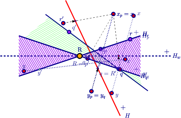
Figure 10: From $(R,p,q)$, we rotate $H_{q}$ anchored at $q=R^{\prime}$ and get the next $(R^{\prime},p^{\prime},q^{\prime})$, but the orientation of $(R^{\prime},p^{\prime},q^{\prime})$ is not defined because the segment $xy$ passes through $R^{\prime}$.

The rotation process is handled by procedures $NextNeighbor$ and $PrevNeighbor$, which we describe next. Let $w=(R,p,q)$ be the current double-wedge. Some abnormal cases may happen in the output $w^{\prime}=(R^{\prime},p^{\prime},q^{\prime})$ of $NextNeighbor$ or $PrevNeighbor$ when the segment $xy$ that defines the orientation of $H_{w^{\prime}}$ passes through $R^{\prime}$ (see Figure 10), $H_{p^{\prime}}$ or $H_{q^{\prime}}$ contains more than $d$ points, or the orientations of $H_{p^{\prime}},H_{q^{\prime}},H_{w^{\prime}}$ are not consistent. For these cases, the path will end or start at $w$. When UniqueEOPL outputs $w$, we can compute $w^{\prime}$ and find the certificate of a violation as follows: for the first or second case, it is easy to see that it violates well-separation and/or weak general position. For the third case, we show that it violates well-separation and that we can obtain a certificate for the violation in Lemma 7.

Procedure $(R^{\prime},p^{\prime},q^{\prime})=NextNeighbor(R,p,q)$

1. Let $w=(R,p,q)$ and let $t_{1}$ be the missing color in $R$.

2. Let $P^{+}_{t_{1}}$ be the subset of $P_{t_{1}}$ that lies in $H^{+}_{w}$ and $P^{-}_{t_{1}}$ be the subset of $P_{t_{1}}$ that lies in $H^{-}_{w}$. Then, let $x\in P^{+}_{t_{1}}$ be the highest ranked point according to the order $\prec_{t_{1}}$ and $y\in P^{-}_{t_{1}}$ be the highest ranked point according to the order $\prec_{t_{1}}$. As we describe previously, $q$ lies on the lower hyperplane.

3. Since $w$ is supposed to be on the canonical path and is not the end point, the $\alpha$-vector of $H_{q}$ is in the form of $(\alpha_{1},\ldots,\alpha_{t_{1}-1},b_{t_{1}},1\ldots,1)$ with $b_{t_{1}}\leq\alpha_{t_{1}}$.

   • If $q$ shares the same color of a point $r$ in $R$, then set $R^{\prime}:=R\cup\{q\}\setminus\{r\}$ and $p^{\prime}:=r$.

   • If $q$ is in color $t_{1}$ and $b_{t_{1}}<\alpha_{t_{1}}$, then set $R^{\prime}:=R$ and $p^{\prime}:=q$.

   • If $q$ is in color $t_{1}$ and $b_{t_{1}}=\alpha_{t_{1}}$, then let $r$ be the point in $R$ with color $t_{1}+1$ and set $R^{\prime}:=R\cup\{q\}\setminus\{r\}$ and $p^{\prime}=r$.

4. We rotate $H_{q}$ around the anchor $R^{\prime}$ in a direction such that the hyperplane is moving away from $x$ along the segment $xy$ until it hits a point $q^{\prime}\in P$.

5. Return $(R^{\prime},p^{\prime},q^{\prime})$.

Procedure $(R^{\prime},p^{\prime},q^{\prime})=PrevNeighbor(R,p,q)$

1. Let $w=(R,p,q)$ and let $t_{1}$ be the missing color in $R$.

2. Let $P^{+}_{t_{1}}$ be the subset of $P_{t_{1}}$ that lies in $H^{+}_{w}$ and $P^{-}_{t_{1}}$ be the subset of $P_{t_{1}}$ that lies in $H^{-}_{w}$. Then, let $x\in P^{+}_{t_{1}}$ be the highest ranked point according to the order $\prec_{t_{1}}$ and $y\in P^{-}_{t_{1}}$ be the highest ranked point according to the order $\prec_{t_{1}}$. As we describe previously, $p$ lies on the upper hyperplane.

3. Since $w$ is supposed to be on the canonical path and is not the starting point, the $\alpha$-vector of $H_{p}$ is in the form of $(\alpha_{1},\ldots,\alpha_{t_{1}-1},b_{t_{1}},1\ldots,1)$ with $b_{t_{1}}\leq\alpha_{t_{1}}$. When $t_{1}=1$, $b_{1}>1$.

   • If $p$ shares the same color of a point $r$ in $R$, then set $R^{\prime}:=R\cup\{p\}\setminus\{r\}$ and $q^{\prime}:=r$.

   • If $p$ is in color $t_{1}$ and $b_{t_{1}}>1$, then set $R^{\prime}:=R$ and $q^{\prime}:=p$.

   • If $p$ is in color $t_{1}$ and $b_{t_{1}}=1$, then let $r$ be the point in $R$ with color $t_{1}-1$ and set $R^{\prime}:=R\cup\{p\}\setminus\{r\}$ and $q^{\prime}=r$.

4. We rotate $H_{p}$ around the anchor $R^{\prime}$ in a direction such that the hyperplane is moving closer to $x$ along the segment $xy$ until it hits a point $p^{\prime}\in P$.

5. Return $(R^{\prime},p^{\prime},q^{\prime})$.

Lemma 15.

The procedures $NextNeighbor(R,p,q)$ and $PrevNeighbor(R,p,q)$ can be completed in $\mathrm{poly}(n,d)$ time.

Proof.

The points $x$ and $y$ from the missing color can be found in linear time. We can also check which point will hit the hyperplane first during the rotation by a prune-and-search technique in polynomial time. ∎

Now we discuss the implementation of $\mathbb{S}$ and $\mathbb{P}$ in $\cal I^{\prime}$. In Procedure $\mathbb{S}$, we first point the standard source $0^{\kappa}$ to the start of the canonical path in Step $\bf\mathbb{S}\hskip 0.28436pt{1}$. For those vertices $(t_{1},\ldots,t_{d+4})$ not on the canonical path, we form self-loops in Steps $\bf\mathbb{S}\hskip 0.28436pt{2}$, $\bf\mathbb{S}\hskip 0.28436pt{3}$ and $\bf\mathbb{S}\hskip 0.28436pt{4}$. After these steps, we check whether we reached the target end point of the canonical path in Step $\bf\mathbb{S}\hskip 0.28436pt{5}$. To handle the violation of weak general position, when a hyperplane $H$ contains more than $d$ points and at least $d-1$ colors, then it happens that several tuples $(R,p,q)$ represents the same double-wedge. We connect all these tuples to form a cycle in Step $\bf\mathbb{S}\hskip 0.28436pt{6}$ when $H$ is the upper hyperplane. If instead $H$ is the lower hyperplane, we handle this in Step $\bf\mathbb{S}\hskip 0.28436pt{7}$. In the end, we use $NextNeighbor$ to advance to the next vertex along the canonical path in Step $\bf\mathbb{S}\hskip 0.28436pt{8}$. As we mentioned previously, if something goes wrong in the next vertex, the path will end in Step $\bf\mathbb{S}\hskip 0.28436pt{9}$. The Procedure $\mathbb{P}$ is basically the same as Procedure $\mathbb{S}$, so we only mention the differences. In Steps $\bf\mathbb{P}\hskip 0.28436pt4$ and $\bf\mathbb{P}\hskip 0.28436pt5$ of $\mathbb{P}$, we ensure a consistent relation between the standard source $0^{\kappa}$ and the start of the canonical path. If there exists another (very) colorful double-wedge with $\alpha$-vector $(1,\ldots,1)$, then it will not connect to $0^{\kappa}$ via $\mathbb{P}$, instead it will be the start of another path.

Procedure $\mathbb{S}(v=(t_{1},\ldots,t_{d+4}))$

1. If $v=0^{\kappa}$, then Return $f_{v}(\{p^{\prime}_{2},\ldots,p^{\prime}_{d}\},p^{\prime}_{1},q^{\prime})$, where $\{p^{\prime}_{1},\ldots,p^{\prime}_{d}\}$ is a colorful point set on a hyperplane $H_{0}$ that has $\alpha$-vector $=(1,\ldots,1)$, and $q^{\prime}$ is the point that creates a double-wedge with the anchor $\{p^{\prime}_{2},\ldots,p^{\prime}_{d}\}$ and $p^{\prime}_{1}$.

2. If $(t_{1},\ldots,t_{d+4})$ is not the encoding of a double-wedge, then Return $(t_{1},\ldots,t_{d+4})$.

3. Let $(R,p,q)$ denote the double-wedge for which $f_{v}(R,p,q)=(t_{1},\ldots,t_{d+4})$. If the orientations of $H_{w}$, $H_{p}$ and $H_{q}$ are not consistent, then Return $f_{v}(R,p,q)$.

4. Recall that $t_{1}$ is the missing color in $R$. If the $\alpha$-vector of $(R,p,q)$ is not in the form of $(\alpha_{1},\ldots,\alpha_{t_{1}-1},b_{t_{1}},1,\ldots,1)$ with $b_{t_{1}}<\alpha_{t_{1}}$, then Return $f_{v}(R,p,q)$.

5. If the $\alpha$-vector of the lower hyperplane $H_{q}$ is $(\alpha_{1},\ldots,\alpha_{d})$, then Return $f_{v}(R,p,q)$.

6. If $H_{p}$ contains some points of $P$ other than $R\cup\{p\}$, then let $p_{1},p_{2},\ldots,p_{m}$ be those extra points ordered by $\prec$, and let $p_{i}$ be the point just after $p$ in the order $\prec$ (if $p$ is after $p_{m}$, then $p_{i}=p_{1}$). We Return $f_{v}(R,p_{i},q)$.

7. Similarly, Return $f_{v}(R,p,q_{i})$ if $H_{q}$ contains some points other than $R\cup\{q\}$, where $q_{i}$ is the point just after $q$ according to the order $\prec$ among those extra points.

8. Let $w^{\prime}=(R^{\prime},p^{\prime},q^{\prime})$ be the output of $NextNeighbor(R,p,q)$. If the orientations of $H_{w^{\prime}}$, $H_{p^{\prime}}$ and $H_{q^{\prime}}$ are well-defined and consistent, then Return $f_{v}(R^{\prime},p^{\prime},q^{\prime})$.

9. Otherwise Return $f_{v}(R,p,q)$.

Procedure $\mathbb{P}(v=(t_{1},\ldots,t_{d+4}))$

1. If $v=0^{\kappa}$, then Return $0^{\kappa}$.

2. If $(t_{1},\ldots,t_{d+4})$ is not a double-wedge, then Return $(t_{1},\ldots,t_{d+4})$.

3. Let $(R,p,q)$ be a double-wedge such that $f_{v}(R,p,q)=(t_{1},\ldots,t_{d+4})$. If the orientations of $H_{w}$, $H_{p}$ and $H_{q}$ are not consistent, then Return $f_{v}(R,p,q)$.

4. If $R=\{p^{\prime}_{2},\ldots,p^{\prime}_{d}\}$ and $p=p^{\prime}_{1}$, then Return $0^{\kappa}$.

5. If $H_{p}$ is colorful, $t_{1}=1$ and the $\alpha$-vector of $H_{p}$ is $(1,\ldots,1)$, then Return $f_{v}(R,p,q)$.

6. Recall that $t_{1}$ is the missing color in $R$. If the $\alpha$-vector of $(R,p,q)$ is not in the form of $(\alpha_{1},\ldots,\alpha_{t_{1}-1},b_{t_{1}},1,\ldots,1)$ with $b_{t_{1}}<\alpha_{t_{1}}$, then Return $f_{v}(R,p,q)$.

7. If $H_{p}$ contains some points of $P$ other than $R\cup\{p\}$, then let $p_{1},p_{2},\ldots,p_{m}$ be those extra points ordered by $\prec$, and let $p_{i}$ be the point just before $p$ in $\prec$ (if $p$ is before $p_{1}$, then $p_{i}=p_{m}$), and Return $f_{v}(R,p_{i},q)$.

8. Similarly, Return $f_{v}(R,p,q_{i})$ if $H_{q}$ contains some points other than $R\cup\{q\}$, where $q_{i}$ is the point just before $q$ in $\prec$ among those extra points.

9. Let $w^{\prime}=(R^{\prime},p^{\prime},q^{\prime})$ be the output of $PrevNeighbor(R,p,q)$. If the orientations of $H_{w^{\prime}}$, $H_{p^{\prime}}$ and $H_{q^{\prime}}$ are well-defined and consistent, then Return $f_{v}(R^{\prime},p^{\prime},q^{\prime})$.

10. Otherwise Return $f_{v}(R,p,q)$.

Given a double-wedge $(R,p,q)$, let $x^{\prime}$ be any point of $P$ in $H^{+}_{p}\cap H^{+}_{q}$ and let $y^{\prime}$ be any point of $P$ in $H^{-}_{p}\cap H^{-}_{q}$. Suppose that the segment $x^{\prime}y^{\prime}$ does not pass through the affine hull of $R$ so that the intersections of $x^{\prime}y^{\prime}$ with $H_{p}$ and $H_{q}$ are two distinct points. Let $d_{\min}$ be the Euclidean distance between the two intersection points of $x^{\prime}y^{\prime}$ with $H_{p}$ and $H_{q}$. Let $d_{\max}$ be the Euclidean distance between $x$ and the intersection point of $x^{\prime}y^{\prime}$ with $H_{q}$.

Lemma 16.

Let $m_{0}$ denote the number of bits needed to represent each coordinate of any point of $P$. Then, $d_{\min}$ is at less $1/N^{2}$ and $d_{\max}$ is at most $M$, where $N=d!2^{dm_{0}}$ and $M=\sqrt{d}2^{m_{0}}$.

Proof.

Without loss of generality, we assume that the missing color in $R$ is color 1, i.e., $R$ is a set of points $\{p_{2}\in P_{2},\ldots,p_{d}\in P_{d}\}$. Let $z_{p}$ (resp. $z_{q}$) be the intersection of $x^{\prime}y^{\prime}$ and $H_{p}$ (resp. $H_{q}$). Since $z_{p}$ lies on $x^{\prime}y^{\prime}$ and the affine hull of $H_{p}$, we can represent $z_{p}$ as the convex combination of $x^{\prime}$ and $y^{\prime}$ and the linear combination of $R\cup\{p\}$ as follows:

$$z_{p}=\lambda_{1}x^{\prime}+(1-\lambda_{1})y^{\prime}=p_{1}+\sum_{i=2}^{d}\lambda_{i}(p_{i}-p_{1}),0\leq\lambda_{1}\leq 1,\lambda_{i}\in\mathbb{R}~{}\forall i\in[2\dots d].$$

Then, we can formulate it as a linear system $A\lambda=b$, where $A\in\mathbb{Z}^{d\times d}$ and $b\in\mathbb{Z}^{d}$:

$$\Bigg{[}y^{\prime}-x^{\prime}~{}|~{}p_{2}-p_{1}~{}|~{}\ldots~{}|~{}p_{d}-p_{1}\Bigg{]}\cdot\Bigg{[}\lambda_{1}~{}|~{}\lambda_{2}~{}|~{}\ldots~{}|~{}\lambda_{d}\Bigg{]}^{t}=y^{\prime}-p_{1},$$

where $y^{\prime}-x^{\prime},p_{2}-p_{1},\dots$ are column vectors. Since we assume that $z_{p}$ exists, we have $\det A\neq 0$. According to Cramer’s rule, we have $\lambda_{i}=\frac{\det A_{i}}{\det A}$, where $A_{i}$ is the matrix obtained by replacing the $i$-th column of $A$ with $b$. Using Leibniz formula for determinants, we can bound the denominator:

$$|\det A|=\bigg{|}\sum_{\sigma\in S_{d}}\mathrm{sgn}(\sigma)\prod_{i=1}^{d}A_{i,\sigma(i)}\bigg{|}\leq d!2^{dm_{0}}=N,$$

where $S_{d}$ is the set of all permutations of $[d]$ and $\mathrm{sgn}(\cdot)$ is the sign function of permutations. The same bound is also applied to $|\det A_{i}|$. Then, $\lambda_{1}=\frac{i}{|\det A|}$ for some $0\leq i\leq|\det A|\leq N$. Similarly, we apply the same argument for $z_{q}$ with another linear system $A^{\prime}\lambda^{\prime}=b^{\prime}$ such that $z_{q}=\lambda^{\prime}_{1}x^{\prime}+(1-\lambda^{\prime}_{1})y^{\prime}$ and $\lambda^{\prime}_{1}=\frac{i^{\prime}}{|\det A^{\prime}|}$. Since $z_{p}$ and $z_{q}$ are two distinct points, at least one of their coordinates, namely $j$, have different values. Therefore, $d_{\min}\geq||z_{p}-z_{q}||\geq\bigg{|}\frac{i}{|\det A|}-\frac{i^{\prime}}{|\det A^{\prime}|}\bigg{|}\cdot(x^{\prime}_{j}-y^{\prime}_{j})\geq\bigg{|}\frac{|\det A^{\prime}|i-|\det A|i^{\prime}}{|\det A|\cdot|\det A^{\prime}|}\bigg{|}\cdot(x^{\prime}_{j}-y^{\prime}_{j})\geq\frac{1}{N^{2}}$. The numerator is at least one because all values are integers.

For $d_{\max}$, it is less than the longest possible line segment, so $d_{\max}\leq\sqrt{d}2^{m_{0}}$. ∎

Using Lemma 16, we can use $\lceil\log_{2}MN^{2}\rceil$ bits to represent the dist-value of any double-wedge so that no two double-wedges on a path of non-colorful vertices of $G$ have the same dist-value. We now define the circuit $\mathbb{V}$ in $\cal I^{\prime}$. We define a potential function $\delta:(R,p,q)\rightarrow\mathbb{Z}$ that measures the distance of $(R,p,q)$ with $\alpha$-vector $(b_{1},\ldots,b_{d})$ and dist-value $D$ to the starting vertex that has $\alpha$-vector $(1,\ldots,1)$. More precisely,

$$\delta(R,p,q)=MN^{2}\cdot\left(\sum_{i=1}^{d}n_{0}^{d-i}(b_{i}-1)\right)+\lfloor DN^{2}\rfloor.$$

Procedure $\mathbb{V}(v=(t_{1},\ldots,t_{d+4}))$

1. If $v=0^{k}$, then Return $0$.

2. If $(t_{1},\ldots,t_{d+4})$ is not a double-wedge, then Return $0$. Otherwise, let $(R,p,q)$ be a double-wedge such that $f_{v}(R,p,q)=(t_{1},\ldots,t_{d+4})$.

3. If $\mathbb{S}(v)=v$ and $\mathbb{P}(v)=v$, then Return $0$.

4. If $\mathbb{S}(v)\neq v$ or $\mathbb{P}(v)\neq v$, then Return $\delta(R,p,q)$.

The following lemma shows that if there are no violations in Alpha-HS, there are also no violations in the constructed UniqueEOPL instance. This makes the reduction promise-preserving. In particular, we can find the $(\alpha_{1},\ldots,\alpha_{d})$-cut from the unique solution of the UniqueEOPL instance.

Lemma 17.

If there are no violations in $\cal I$, then the constructed UniqueEOPL instance $\cal I^{\prime}$ only contains a type (U1) solution whose lower hyperplane is colorful and has $\alpha$-vector $=(\alpha_{1},\ldots,\alpha_{d})$, which is a type (G1) solution of $\cal I$.

Proof.

First we show that there must exist a type (U1) solution whose lower hyperplane has $\alpha$-vector $=(\alpha_{1},\ldots,\alpha_{d})$. If there are no violations in $\cal I$, then by Theorem 2 there exists a unique colorful hyperplane $H$ passing through some $p_{1}\in P_{1},\ldots,p_{d}\in P_{d}$ with $\alpha$-vector $\alpha=(\alpha_{1},\ldots,\alpha_{d})$. Let $i$ be the largest index of the coordinates in $\alpha$ such that $\alpha_{i}\neq 1$. Define $R=(p_{1},\ldots,p_{i-1},p_{i+1},\ldots,p_{d})$. Similar to Procedure $PrevNeighbor$, we rotate $H$ around the anchor $R$ in a direction such that $p_{i}$ is in the open half-space $H^{-}$ until the hyperplane hits a point $q\in P$. Define $w=(R,q,p_{i})$. Since $P$ is well-separated and in weak general position, the orientations of $H_{p},H_{q},H_{w}$ are well-defined and consistent. Furthermore, $p_{i}$ is on the lower hyperplane of $w$. That means, $w$ is a double-wedge. In particular, the $\alpha$-vector of $w$ is $(\alpha_{1},\ldots,\alpha_{i}-1,1,\ldots,1)$. Similarly, we can also define a double-wedge $w_{0}$ as shown in Step $\bf\mathbb{S}\hskip 0.28436pt{1}$ of Procedure $\mathbb{S}$, which has $\alpha$-vector $=(1,\ldots,1)$ and has $H_{0}$ as the upper hyperplane.

Following the definition of the canonical path in Section 3.1, we can define the canonical path between $w_{0}$ and $w$, in which every vertex on the path is a double-wedge with $\alpha$-vector in the form of $(\alpha_{1},\ldots,\alpha_{t_{1}-1},b_{t_{1}},1,\ldots,1)$ for some $b_{t_{1}}<\alpha_{t_{1}}$, where $t_{1}\leq i$ is the missing color of the anchor of the double-wedge, and every two consecutive double-wedges share a hyperplane. This canonical path is realized by Step $\bf\mathbb{S}\hskip 0.28436pt{8}$ of Procedure $\mathbb{S}$ and Step $\bf\mathbb{P}\hskip 0.28436pt9$ of Procedure $\mathbb{P}$. Since the lower hyperplane $H_{p_{i}}$ has $\alpha$-vector $=(\alpha_{1},\ldots,\alpha_{d})$, Procedure $\mathbb{S}(f_{v}(w))$ will return at Step $\bf\mathbb{S}\hskip 0.28436pt{5}$ so that $\mathbb{P}(\mathbb{S}(f_{v}(w)))=\mathbb{P}(f_{v}(w))\neq f_{v}(w)$ and $f_{v}(w)$ is a type (U1) solution.

Next we will show that there do not exist other solutions. As we mentioned above, we only construct a single path from $0^{\kappa}$ to $f_{v}(w_{0})$ and then to $f_{v}(w)$. For other double-wedges not on the path, they will form a self-loop by Step $\bf\mathbb{S}\hskip 0.28436pt{4}$ of Procedure $\mathbb{S}$ and Step $\bf\mathbb{P}\hskip 0.28436pt6$ of Procedure $\mathbb{P}$. For non-double-wedges, they will also form a self-loop by Step $\bf\mathbb{S}\hskip 0.28436pt{2}$ of Procedure $\mathbb{S}$ and Step $\bf\mathbb{P}\hskip 0.28436pt2$ of Procedure $\mathbb{P}$. When $P$ is well-separated and in weak general position, the orientations of all double-wedges are well-defined and consistent as shown in Lemma 7. Therefore, Procedure $\mathbb{S}$ will not return at Steps $\bf\mathbb{S}\hskip 0.28436pt{3}$, $\bf\mathbb{S}\hskip 0.28436pt{6}$, $\bf\mathbb{S}\hskip 0.28436pt{7}$ and $\bf\mathbb{S}\hskip 0.28436pt{9}$, and Procedure $\mathbb{P}$ will also not return at Steps $\bf\mathbb{P}\hskip 0.28436pt3$, $\bf\mathbb{P}\hskip 0.28436pt7$, $\bf\mathbb{P}\hskip 0.28436pt8$ and $\bf\mathbb{P}\hskip 0.28436pt10$. Since there is only one colorful hyperplane with $\alpha$-vector $=(1,\ldots,1)$, Procedure $\mathbb{P}$ will not return at Step $\bf\mathbb{P}\hskip 0.28436pt5$. ∎

There are different types of violations that may return from a UniqueEOPL instance. To obtain the certificate of violation (GV1) in Alpha-HS, we need the following lemmas to convert the violation solutions of UniqueEOPL to the (GV1) certificate.

Lemma 18.

Given $\{x_{1}\in\mathrm{conv}(P_{1}),\dots,x_{d}\in\mathrm{conv}(P_{d})\}$ that spans a hyperplane $H$. For any point $y$ in the open halfspace $H^{+}$,

$$\mathrm{det}\begin{vmatrix}x_{1}&x_{2}&\dots&x_{d}&y\\ 1&1&\dots&1&1\end{vmatrix}>0.$$

Similarly, for any point $y$ in the open halfspace $H^{-}$,

$$\mathrm{det}\begin{vmatrix}x_{1}&x_{2}&\dots&x_{d}&y\\ 1&1&\dots&1&1\end{vmatrix}<0.$$

Proof.

The normal $\hat{n}$ that defines the orientation of $H$ satisfies $\mathrm{det}\begin{vmatrix}x_{1}&x_{2}&\dots&x_{d}&\hat{n}\\ 1&1&\dots&1&0\end{vmatrix}>0.$ For any point $y$ in the open halfspace $H^{+}$, let $\bar{y}$ be the orthogonal projection of $y$ onto $H$, i.e., $\bar{y}=\sum_{i=2}^{d}\lambda_{i}(x_{i}-x_{1})+x_{1}$ and $y=\bar{y}+\gamma\hat{n}$ for some positive number $\gamma$. Then, we have

$$\mathrm{det}\begin{vmatrix}x_{1}&x_{2}&\dots&x_{d}&y\\ 1&1&\dots&1&1\end{vmatrix}$$

$$= \mathrm{det}\begin{vmatrix}x_{1}&x_{2}&\dots&x_{d}&\bar{y}+\gamma\hat{n}\\ 1&1&\dots&1&1\end{vmatrix}$$

$$= \mathrm{det}\begin{vmatrix}x_{1}&x_{2}&\dots&x_{d}&\hat{y}-x_{1}+\gamma\hat{n}\\ 1&1&\dots&1&0\end{vmatrix}$$

$$= \mathrm{det}\begin{vmatrix}x_{1}&x_{2}&\dots&x_{d}&\gamma\hat{n}\\ 1&1&\dots&1&0\end{vmatrix}>0.$$

The proof for points in the open halfspace $H^{-}$ is similar. ∎

By Theorem 2, we already know that if there are multiple $\alpha$-cuts, then $P$ is not well-separated. The following two lemmas give the same result, but we provide a constructive proof so that we can find the certificate of the violation.

Lemma 19.

Given two colorful hyperplanes $H_{p}$, $H_{q}$ that have the same $\alpha$-vector such that $H_{p}\cap H_{q}$ does not intersect $\mathrm{conv}(P_{i})$ for all $i\in[d]$, we can find a colorful set of points $\{x_{1}\in\mathrm{conv}(P_{1}),\ldots,x_{d}\in\mathrm{conv}(P_{d})\}$ that lies on a $(d-2)$-flat in $\mathrm{poly}(n,d,m_{0})$ time, which shows that $P$ is not well-separated.

Proof.

The proof is based on the idea of finding a hyperplane that ”interpolates” between $H_{p}$ and $H_{q}$, for which no consistent orientation can be defined. This hyperplane gives the certificate of violation.

Let $p_{1}\in P_{1},\ldots,p_{d}\in P_{d}$ denote the colorful points on $H_{p}$ and $q_{1}\in P_{1},\ldots,q_{d}\in P_{d}$ denote the colorful points on $H_{q}$.

Claim 20.

The open segment $p_{i}q_{i}$ is contained in either $H_{p}^{+}\cap H_{q}^{+}$ or $H_{p}^{-}\cap H_{q}^{-}$ for each $i\in[d]$.

Proof.

Since $H_{p}\cap H_{q}$ does not intersect $\mathrm{conv}(P_{i})$ and both $H_{p},H_{q}$ intersect $\mathrm{conv}(P_{i})$, $H_{p}$ and $H_{q}$ cut $\mathrm{conv}(P_{i})$ into three cells for each $i\in[d]$. Suppose that the middle cell is in $H_{p}^{-}\cap H_{q}^{+}$. Then, $P_{i}\cap H_{p}^{+}\subseteq P_{i}\cap H_{q}^{+}$. Since $q_{i}\notin H_{p}^{+}$, then we have $|P_{i}\cap H_{q}^{+}|>|P_{i}\cap H_{p}^{+}|$, which contradicts the assumption that $H_{p}$ and $H_{q}$ share their $\alpha$-vectors. The same argument applies to $H_{p}^{+}\cap H_{q}^{-}$. It is straightforward to see that $p_{i}q_{i}$ is contained in the middle cell, which is either $H_{p}^{+}\cap H_{q}^{+}$ or $H_{p}^{-}\cap H_{q}^{-}$. ∎

Let $R$ denote the intersection of $H_{p}\cap H_{q}$ and $\theta_{0}$ denote the angle between $H_{p}$ and $H_{q}$ with respect to $H_{p}^{+}\cap H_{q}^{+}$. Let $H(\theta)$ denote the hyperplane that rotates anchored at $R$ from $H_{p}$ to $H_{q}$ inside the region $(H_{p}^{+}\cap H_{q}^{+})\cup(H_{p}^{-}\cap H_{q}^{-})$ with $\theta$ denoting the angle to $H_{p}$. By Claim 20, $H(\theta)$ intersects $p_{i}q_{i}$ for all $i\in[d]$. Let $z_{i}(\theta)$ denote that intersection. We can see that $z_{i}(\theta)$ changes continuously with $\theta$. Let $r$ be any point of $\mathbb{R}^{d}$ in the open cell $H_{p}^{+}\cap H_{q}^{-}$ that $r$ does not lie on $H(\theta)$ for $0\leq\theta\leq\theta_{0}$. Notice that $r-z_{1}(\theta)$ is linearly independent of the vectors $\{z_{i}(\theta)-z_{1}(\theta),\forall i\in[2..d]\}$. Let $Det(\theta)=\mathrm{det}\begin{vmatrix}z_{1}(\theta)&z_{2}(\theta)&\dots&z_{d}(\theta)&r\\ 1&1&\dots&1&1\end{vmatrix}$, which is a continuous function for $0\leq\theta\leq\theta_{0}$. Since $r\in H_{p}^{+}\cap H_{q}^{-}$, by the definition of the orientation and Lemma 18, $Det(0)>0$ and $Det(\theta_{0})<0$. From the intermediate value theorem, there exists $0\leq\theta^{\prime}\leq\theta_{0}$ for which $Det(\theta^{\prime})=0$. Thus, we have

$$0 = \mathrm{det}\begin{vmatrix}z_{1}(\theta^{\prime})&z_{2}(\theta^{\prime})&\dots&z_{d}(\theta^{\prime})&r\\ 1&1&\dots&1&1\end{vmatrix}$$

$$= \mathrm{det}\begin{vmatrix}z_{1}(\theta^{\prime})&z_{2}(\theta^{\prime})-z_{1}(\theta^{\prime})&\dots&z_{d}(\theta^{\prime})-z_{1}(\theta^{\prime})&r-z_{1}(\theta^{\prime})\\ 1&0&\dots&0&0\end{vmatrix}$$

$$= (-1)^{d+2}\cdot\mathrm{det}\begin{vmatrix}z_{2}(\theta^{\prime})-z_{1}(\theta^{\prime})&\dots&z_{d}(\theta^{\prime})-z_{1}(\theta^{\prime})&r-z_{1}(\theta^{\prime})\\ \end{vmatrix}$$

Since $r-z_{1}(\theta^{\prime})$ is linearly independent of the vectors $\{z_{i}(\theta^{\prime})-z_{1}(\theta^{\prime}),\forall i\in[2\dots d]\}$, we see that $\mathrm{span}(\{z_{i}(\theta^{\prime})-z_{1}(\theta^{\prime}),\forall i\in[2\dots d]\})$ has dimension at most $d-2$. Hence, the colorful set $\{z_{i}(\theta^{\prime})\mid i\in[d]\}$ lies on a $(d-2)$-flat. To compute $\{z_{i}(\theta^{\prime})\mid i\in[d]\}$, we use binary search on the interval $[0,\theta_{0}]$ to find $\theta^{\prime}$. ∎

(a) The point $y$ is in the convex hulls of colors 1 (purple) and 2 (yellow).

(b) The point $x$ lies in both triangles $\triangle p_{1}q_{1}r_{1}$ and $\triangle p_{2}q_{2}r_{2}$.

(c) The point $p_{2}$ lies in the triangle $\triangle p_{1}q_{1}r_{1}$.

Figure 11: Some figures for Lemma 8.

We now extend Lemma 8 to the case where the two hyperplanes are non-colorful but have the same $\alpha$-vector and dist-value. On any path of non-colorful vertices of $G$ that starts and ends at colorful vertices, the dist-values of the vertices along the path is bounded by the dist-values of the two end points. Hence, we have an interval of the dist-values along the path with respect to an $\alpha$-vector $(\alpha_{1},\ldots,\alpha_{i-1},b_{i},1,\ldots,1)$, where $i$ is the missing color for those non-colorful vertices and $b_{i}<\alpha_{i}$. If we find another non-colorful vertex with the same missing color and $\alpha$-vector but its dist-value is outside the interval, we show that it implies a violation of well-separation in the following lemma.

Lemma 21.

Given a double-wedge $w=(R,r,q)$ with a colorful lower hyperplane $H_{q}$ and a non-colorful hyperplane $H$ such that $H_{w}$ and $H$ have the same missing color and $\alpha$-vector, but the dist-value of $H$ is larger than that of $H_{q}$, we can find a colorful set $\{x_{1}\in\mathrm{conv}(P_{1}),\ldots,x_{d}\in\mathrm{conv}(P_{d})\}$ that lies on a $(d-2)$-flat in $\mathrm{poly}(n,d,m_{0})$ time.

Proof.

Without loss of generality, we assume that the missing color of $H_{w}$ and $H$ is color $1$. Let $p_{2}\in P_{2},\ldots,p_{d}\in P_{d}$ be the colorful points on $H$ and $q_{2}\in P_{2},\ldots,q_{d}\in P_{d}$ be the colorful points on $H_{w}$. Let $x_{p},y_{p}$ (resp. $x_{q},y_{q}$) be the highest ranked points of $P_{1}$ under $\prec_{1}$ on either side of $H$ (resp. $H_{w}$) As we saw in the proof of Lemma 9, the condition that the hyperplanes share the dist-value is required only in the first case when $x_{p},x_{q}\in H^{+}\cap H_{w}^{+}$ and $y_{p},y_{q}\in H^{-}\cap H_{w}^{-}$. We can apply the same analysis from Lemma 9 for $H$ and $H_{w}$ in other cases.

When $x_{p},x_{q}\in H^{+}\cap H_{w}^{+}$ and $y_{p},y_{q}\in H^{-}\cap H_{w}^{-}$, we have $x_{p}=x_{q}$ and $y_{p}=y_{q}$. Since $H_{w}$ is the representative hyperplane, $H_{q}$ is the lower hyperplane and the dist-value of $H$ is larger than that of $H_{q}$, the directed segment $x_{q}y_{q}$ intersects them in the following order: $H_{w}$, $H_{q}$ then $H$. Since $w$ is a double-wedge, the orientations of $H_{w}$ and $H_{q}$ are consistent. That means, $q\in H_{q}\cap H_{w}^{-}$. There are two possibilities:

• $q\in H^{+}\cap H_{w}^{-}$: using a similar argument as in the proof of Lemma 9, there must exist another point $r^{\prime}\in P_{1}\cap H^{-}\cap H_{w}^{+}$ because $q\in P_{1}$ and $H,H_{w}$ have the same $\alpha$-vector. Then, we move $q$ towards $x_{p}$ along segment $x_{p}q$ until it hits $H_{w}$ and move $r^{\prime}$ towards $x_{p}$ along segment $x_{p}r^{\prime}$ until it hits $H$ (Figure 12(a)). We apply Lemma 8 to the resulting point set and that completes the proof.

• $q\in H^{-}\cap H_{w}^{-}$: in this case both $y_{q}$ and $q$ lie in $q\in H^{-}\cap H_{w}^{-}$, but $y_{q}\neq q$ since that would make the intersection order along $x_{q}y_{q}$ as $H_{w},H,H_{q}$, which is a contradiction. Along the directed segment $x_{q}q$, the order of intersection is $H,H_{w}$ (Figure 12(b)) while on the directed segment $x_{q}y_{q}$ it is $H_{w},H$. So we move $y_{q}$ towards $x_{q}$ along $x_{q}y_{q}$ until it hits $H$, and move $q$ towards $x_{q}$ along $x_{q}q$ until it hits $H_{w}$. Then we re-use the proof from Lemma 8.

Thus, the claim is proven. ∎

(a) When $q\in H^{+}\cap H_{w}^{-}$, there exists a point $r^{\prime}\in P_{1}\cap H^{-}\cap H_{w}^{+}$. We move $r^{\prime}$ and $q$ onto $H$ and $H_{w}$ respectively.

(b) When $q\in H^{-}\cap H_{w}^{-}$, we move $y_{q}$ and $q$ onto $H$ and $H_{w}$ respectively.

Figure 12: Some figures for Lemma 21. The small red points represent the new positions after moving those points.

In fact, the conditions in Lemmas 8, 9 and 21 can also serve as certificates of violation of well-separation. Because we want to simplify the statement in (GV2), from the results of Lemmas 8, 9 and 21 we find a colorful set that lies on a $(d-2)$-flat, and then we apply Lemma 1 to compute the index sets $I,J$ as a type (GV2) solution. The reason for not choosing a colorful set as a certificate is that the representation of $I,J$ needs fewer bits than that for a colorful set. Moreover, the bit representation of the violating colorful set may not guarantee that they lie on a $(d-2)$-flat because of the rounding error. Since most of the computations are done by solving linear systems, we believe that a violating colorful set can be represented by $\mathrm{poly}(n,d,m_{0})$ bits. If this fails, we could find a set of feasible solutions that lie very close to a $(d-2)$-flat. Then, we can project the set onto the $(d-2)$-flat and one could argue that Lemma 1 would give a correct partition $(I,J)$.

In the following lemmas, we show how to reduce any violation solution of $\cal I^{\prime}$ to a violation solution of $\cal I$ to complete the reduction.

Lemma 22.

Let $v$ be a type (U1) solution of the constructed UniqueEOPL instance $\cal I^{\prime}$ for which the lower hyperplane has $\alpha$-vector different from the target vector $(\alpha_{1},\ldots,\alpha_{d})$. Then, we can compute a type (GV1) or (GV2) solution of Alpha-HS instance $\cal I$ in $\mathrm{poly}(n,d,m_{0})$ time.

Proof.

By the definition of (U1), we have $\mathbb{P}(\mathbb{S}(v))\neq v$, so $v$ is not on a self-loop or a cycle. Also, $v$ cannot be $0^{\kappa}$. Therefore, $\mathbb{S}(v)$ cannot be returned at Items $\bf\mathbb{S}\hskip 0.28436pt{1}$, $\bf\mathbb{S}\hskip 0.28436pt{2}$, $\bf\mathbb{S}\hskip 0.28436pt{3}$ and $\bf\mathbb{S}\hskip 0.28436pt{4}$. Since the lower hyperplane has $\alpha$-vector $\neq(\alpha_{1},\ldots,\alpha_{d})$, $\mathbb{S}(v)$ also cannot be returned at Step $\bf\mathbb{S}\hskip 0.28436pt{5}$.

There is a special case that Step $\bf\mathbb{S}\hskip 0.28436pt{6}$ ($\bf\mathbb{S}\hskip 0.28436pt{7}$) does not form a cycle, which happens when the hyperplane that contains more than $d$ points and $d$ colors also witnesses a violation of well-separation. The orientation could flip when moving along the path that contains the vertices corresponding to the same double-wedge, so the output $\mathbb{S}(v)$ from Step $\bf\mathbb{S}\hskip 0.28436pt{6}$ ($\bf\mathbb{S}\hskip 0.28436pt{7}$) is not a valid double-wedge. We can verify this case by checking whether the upper or lower hyperplane of $\mathbb{S}(v)$ contains more than $d$ points, which is a type (GV1) solution.

Now we consider Steps $\bf\mathbb{S}\hskip 0.28436pt{8}$ and $\bf\mathbb{S}\hskip 0.28436pt{9}$. There are two possibilities to get $\mathbb{P}(\mathbb{S}(v))\neq v$:

• Case 1: $\mathbb{S}(v)=u\neq v$ and $\mathbb{P}(u)\neq v$, and

• Case 2: $\mathbb{S}(v)=v$ and $\mathbb{P}(v)=u\neq v$.

For Case 1, $u$ is returned at Step $\bf\mathbb{S}\hskip 0.28436pt{8}$, which implies that the orientations of $v$ and $u$ are consistent. Next we consider where $\mathbb{P}(u)$ is returned. From the definition of $NextNeighbor$ and the if-condition of Step $\bf\mathbb{S}\hskip 0.28436pt{8}$, $u$ is a double-wedge with consistent orientations and on the canonical path. Hence, $\mathbb{P}(u)$ cannot be returned at Items $\bf\mathbb{P}\hskip 0.28436pt1$, $\bf\mathbb{P}\hskip 0.28436pt2$, $\bf\mathbb{P}\hskip 0.28436pt3$, $\bf\mathbb{P}\hskip 0.28436pt4$, $\bf\mathbb{P}\hskip 0.28436pt5$ and $\bf\mathbb{P}\hskip 0.28436pt6$. If $\mathbb{P}(u)$ is returned at Step $\bf\mathbb{P}\hskip 0.28436pt9$ or $\bf\mathbb{P}\hskip 0.28436pt10$, we claim that it is not possible. According to Procedure $NextNeighbor$ and Procedure $PrevNeighbor$, since the rotational direction is determined by the orientation of the representative hyperplane, $PrevNeighbor(u)$ should return $v$. Then, we have $\mathbb{P}(u)=v$, which contradicts with the assumption of Case 1. Therefore, the only possibilities of returning are Steps $\bf\mathbb{P}\hskip 0.28436pt7$ and $\bf\mathbb{P}\hskip 0.28436pt8$. Then, we check whether the upper or lower hyperplane of $u=\mathbb{S}(v)$ contains more than $d$ points, which is a type (GV1) solution.

For Case 2, let $w^{\prime}=(R^{\prime},p^{\prime},q^{\prime})$ be the output of $NextNeighbor(v)$. Since $\mathbb{S}(v)=v$, which is returned at Step $\bf\mathbb{S}\hskip 0.28436pt{9}$, the orientations of $H_{p^{\prime}}$, $H_{q^{\prime}}$ and $H_{w^{\prime}}$ are either not well-defined or inconsistent. For the case that the orientations are not well-defined, the segment $xy$ from the missing color of $R^{\prime}$ intersects the flat of $R^{\prime}$, so that the intersection point and $R^{\prime}$ are a type (GV1) solution as well as the index set of the missing color in $R^{\prime}$ and the index set of other colors are a type (GV2) solution. For the other case of inconsistent orientations, by Lemma 7, we can find a type (GV2) solution. ∎

The next lemma is to handle type (UV1) solutions that capture a vertex at which the potential value is not increasing. From the way we construct the graph, it only happens when the weak general position fails.

Lemma 23.

Let $v$ be a type (UV1) solution of the constructed UniqueEOPL instance $\cal I^{\prime}$. Then, a type (GV1) solution of $\cal I$ can be computed in $\mathrm{poly}(n,d)$ time.

Proof.

By the definition of (UV1), we have $\mathbb{S}(v)\neq v$, $\mathbb{P}(\mathbb{S}(v))=v$ and $\mathbb{V}(\mathbb{S}(v))-\mathbb{V}(v)\leq 0$ so $v$ is neither on a self-loop nor an end point of a path. Hence, $\mathbb{S}(v)$ cannot be returned at Items $\bf\mathbb{S}\hskip 0.28436pt{2}$, $\bf\mathbb{S}\hskip 0.28436pt{3}$, $\bf\mathbb{S}\hskip 0.28436pt{4}$, $\bf\mathbb{S}\hskip 0.28436pt{5}$ and $\bf\mathbb{S}\hskip 0.28436pt{9}$. The remaining possibilities are Items $\bf\mathbb{S}\hskip 0.28436pt{1}$, $\bf\mathbb{S}\hskip 0.28436pt{6}$, $\bf\mathbb{S}\hskip 0.28436pt{7}$ and $\bf\mathbb{S}\hskip 0.28436pt{8}$. Since $\mathbb{S}(0^{\kappa})$ has $\alpha$-vector $=(1,\ldots,1)$ and dist-value $>0$, $\mathbb{V}(\mathbb{S}(0^{\kappa}))>\mathbb{V}(0^{\kappa})$, so Item $\bf\mathbb{S}\hskip 0.28436pt{1}$ is also not possible. From the way we rotate the hyperplane in Procedure $NextNeighbor$ and the consistent orientations of $v$ and $\mathbb{S}(v)$ that are confirmed by a return from Item $\bf\mathbb{S}\hskip 0.28436pt{8}$, we can see that $\mathbb{V}(\mathbb{S}(v))>\mathbb{V}(v)$, that is, Step $\bf\mathbb{S}\hskip 0.28436pt{8}$ is not possible. Overall, $\mathbb{V}(\mathbb{S}(v))-\mathbb{V}(v)\leq 0$ can only happen when $\mathbb{S}(v)$ returns at Step $\bf\mathbb{S}\hskip 0.28436pt{6}$ or $\bf\mathbb{S}\hskip 0.28436pt{7}$, which implies that $v$ and $\mathbb{S}(v)$ represent the same double-wedge geometrically so that they have the same potential value. Let $f_{v}(R,p,q)=v$. By checking $H_{p}$ and $H_{q}$, at least one of them would contain another point in $P$, which is a type (GV1) solution. ∎

A solution of type (UV2) means that there is another starting point of some other path. The proof of the following lemma is basically the same as Lemma 22.

Lemma 24.

Let $v$ be a type (UV2) solution of the constructed UniqueEOPL instance $\cal I^{\prime}$. Then, a type (GV1) or (GV2) solution of $\cal I$ can be computed in $\mathrm{poly}(n,d,m_{0})$ time.

Proof.

By the definition of (UV2), we have $\mathbb{S}(\mathbb{P}(v))\neq v\neq 0^{n}$, which implies that $v$ is the starting point of another path. Following the same reasons as in Lemma 22, we can show that $\mathbb{P}(v)$ cannot be returned at Items $\bf\mathbb{P}\hskip 0.28436pt1$, $\bf\mathbb{P}\hskip 0.28436pt2$, $\bf\mathbb{P}\hskip 0.28436pt3$, $\bf\mathbb{P}\hskip 0.28436pt4$ and $\bf\mathbb{P}\hskip 0.28436pt6$. The same special case can also happen at Step $\bf\mathbb{P}\hskip 0.28436pt7$ or $\bf\mathbb{P}\hskip 0.28436pt8$. Hence, we check whether the upper or lower hyperplane of $\mathbb{P}(v)$ contains more than $d$ points, which is a type (GV1) solution.

Let $f_{v}(R,p,q)=v$. When $\mathbb{P}(v)$ is returned at Step $\bf\mathbb{P}\hskip 0.28436pt5$, $H_{p}$ is colorful with $\alpha$-vector $(1,\ldots,1)$ and the missing color of $R$ is color $1$. Since $\mathbb{P}(v)$ did not return at Step $\bf\mathbb{P}\hskip 0.28436pt4$, the standard starting hyperplane $H_{0}$ and $H_{p}$ are two different colorful hyperplanes with the same $\alpha$-vector. Applying Lemma 8 and then Lemma 1, we can find the index sets $I,J$ as a type (GV2) solution.

For the case of Steps $\bf\mathbb{P}\hskip 0.28436pt9$ and $\bf\mathbb{P}\hskip 0.28436pt10$, it is similar to the proof of Lemma 22. There are two possible cases in which $\mathbb{S}(\mathbb{P}(v))\neq v\neq 0^{n}$:

• Case 1: $\mathbb{P}(v)=u\neq v$ and $\mathbb{S}(u)\neq v$, and

• Case 2: $\mathbb{P}(v)=v$ and $\mathbb{S}(v)=u\neq v$.

For Case 1, we apply the same argument in the proof of Lemma 22 to show that the case is impossible. For Case 2, let $w^{\prime}=(R^{\prime},p^{\prime},q^{\prime})$ be the output of $PrevNeighbor(v)$. The orientations of $w^{\prime}$ are not well-defined or inconsistent, then we can find a type (GV2) solution. ∎

In (UV3), either we have two representative hyperplanes with the same potential value, or we find a hyperplane whose potential value is between the potential values of two consecutive representative hyperplanes in $G$. We use Lemmas 9 and 21 to find a violation solution of Alpha-HS.

Lemma 25.

Let $v$ and $u$ be a type (UV3) solution of the constructed UniqueEOPL instance $\cal I^{\prime}$. Then, a type (GV1) or (GV2) solution of $\cal I$ can be computed in $\mathrm{poly}(n,d,m_{0})$ time.

Proof.

By the definition of (UV3), we have $v\neq u$, $\mathbb{S}(v)\neq v$, $\mathbb{S}(u)\neq u$, and either $\mathbb{V}(v)=\mathbb{V}(u)$ or $\mathbb{V}(v)<\mathbb{V}(u)<\mathbb{V}(\mathbb{S}(v))$, so $v,u$ are not on self-loops, that is, $\mathbb{S}(v)$ and $\mathbb{S}(u)$ are not returned at Items $\bf\mathbb{S}\hskip 0.28436pt{2}$, $\bf\mathbb{S}\hskip 0.28436pt{3}$ and $\bf\mathbb{S}\hskip 0.28436pt{4}$. Hence, $v$ may be $0^{\kappa}$ or the $\alpha$-vectors of $v,u$ are in the form of $(\alpha_{1},\ldots,\alpha_{t_{1}-1},b_{t_{1}},1,\ldots,1)$, where $t_{1}$ is the missing color of the anchor $R$ and $b_{t_{1}}<\alpha_{t_{1}}$. For the first case $\mathbb{V}(v)=\mathbb{V}(u)$, $v$ cannot be $0^{\kappa}$. $v$ and $u$ may represent the same double-wedge because of the violation of weak general position. We check whether the upper or lower hyperplanes of $v,u$ contain more than $d$ points in $P$. If yes, we can return $d+1$ points on that hyperplane as a type (GV1) solution. Otherwise, from the way we define $\mathbb{V}$ we know that $H_{v}$ and $H_{u}$ have the same missing color, $\alpha$-vector and dist-value. By Lemma 9 and then Lemma 1, we can find a type (GV2) solution.

For the second case $\mathbb{V}(v)<\mathbb{V}(u)<\mathbb{V}(\mathbb{S}(v))$, $\mathbb{S}(v)$ can only be returned by Step $\bf\mathbb{S}\hskip 0.28436pt{1}$ or $\bf\mathbb{S}\hskip 0.28436pt{8}$ to increase the potential value $\mathbb{V}(v)<\mathbb{V}(\mathbb{S}(v))$. The idea is to find a hyperplane $H$ inside the double-wedge $v$ or $\mathbb{S}(v)$ such that the dist-value of $H$ is the same as that of $H_{u}$. When $v=0^{\kappa}$, both $\mathbb{S}(v)$ and $u$ have $\alpha$-vector $(1,\ldots,1)$ and the dist-value of $u$ is between $0$ and the dist-value of $H_{S(v)}$. Let $f_{v}(R^{\prime},p^{\prime},q^{\prime})=\mathbb{S}(v)$. During the rotation of a hyperplane from $H_{p^{\prime}}$ to $H_{S(v)}$ anchored at $R^{\prime}$, we can find an intermediate hyperplane $H$ that has the same missing color, $\alpha$-vector and dist-value as $H_{u}$. If $v$ and $\mathbb{S}(v)$ share a non-colorful hyperplane, then $H_{v}$ and $H_{\mathbb{S}(v)}$ have the same missing color and $\alpha$-vector. By the definition of $\mathbb{V}$, $H_{u}$ also has the same missing color and $\alpha$-vector. Therefore, the dist-value of $H_{u}$ is between the dist-values of $H_{v}$ and $H_{\mathbb{S}(v)}$. We apply the same idea as above to rotate a hyperplane within the double-wedges $v$ and $\mathbb{S}(v)$ to find a hyperplane $H$ that has the same missing color, $\alpha$-vector and dist-value as $H_{u}$. For the other case when both $v$ and $\mathbb{S}(v)$ share a colorful hyperplane, the $t_{1}$-th coordinate of the $\alpha$-vector of $\mathbb{S}(v)$ is increased by 1 comparing to that of $v$, where $t_{1}$ is the missing color of the anchor $R$ of $v$. If $u$ has the same $\alpha$-vector as $\mathbb{S}(v)$, then the dist-value of $H_{u}$ is between $0$ and the dist-value of $H_{\mathbb{S}(v)}$. We can find a hyperplane $H$ inside the double-wedge $\mathbb{S}(v)$ that has the same missing color, $\alpha$-vector and dist-value as $H_{u}$. If $u$ has the same $\alpha$-vector as $v$ and the dist-value of $u$ is at most the dist-value of the lower hyperplane of $v$, we can still find $H$ in the same way as above. In all these cases, we can apply Lemma 9 on $H$ and $H_{u}$ and then apply Lemma 1 to find a type (GV2) solution. Otherwise, we have that the dist-value of $u$ is larger than the dist-value of the colorful lower hyperplane of $v$. Now $v$ and $H_{u}$ satisfy the condition of Lemma 21 and we again apply Lemma 1 to find a type (GV2) solution. ∎

Now we discuss how to find $H_{0}$. We pick any transversal hyperplane $H^{\prime\prime}$ passing through some colorful set $p^{\prime\prime}_{1}\in P_{1},\ldots,p^{\prime\prime}_{d}\in P_{d}$. Let $b=(b_{1},\ldots,b_{d})$ denote the $\alpha$-vector for $H^{\prime\prime}$. Without loss of generality, we rearrange the order of the colors such that all $b_{i}\neq 1$ occupy the first few coordinates of the $\alpha$-vector. Let $k$ denote the number of coordinates of $b$ that not equal to one. Let $R=(p^{\prime\prime}_{1},\ldots,p^{\prime\prime}_{k-1},p^{\prime\prime}_{k+1},\ldots,p^{\prime\prime}_{d})$. We search for a point $q\in P$ such that $(R,p^{\prime\prime}_{k},q)$ is a double-wedge with $\alpha$-vector $b=(b_{1},\ldots,b_{d})$. Basically, we reverse the roles of $H_{0}$ and $H^{\prime\prime}$ as in the above reduction so that the standard vertex $0^{\kappa}$ connects to $v_{b}=f_{v}(R,p^{\prime\prime}_{k},q)$ and we look for the end vertex $v_{0}$ corresponding to $H_{0}$. If there are no violations in $\cal I$, there exists a canonical path between $v_{b}$ and $v_{0}$. Similarly, we reverse the roles of $\mathbb{S}$ and $\mathbb{P}$, and $\mathbb{V}$ is now the function that measures the distance of the current vertex $(R,p,q)$ with $\alpha$-vector and dist-value to the starting vertex $v_{b}$ that has $\alpha$-vector $(b_{1},\ldots,b_{d})$. If $H_{0}$ cannot be found from the reduction, we can apply the same argument in Lemmas 22, 23, 24 and 25 to output a type (GV1) or (GV2) solution of $\cal I$.

6 Conclusion and future work

We gave a complexity-theoretic upper bound for Alpha-HS. No hardness results are known for this search problem, and the next question is determining if this is hard for $\mathsf{UEOPL}$. One challenge is that UniqueEOPL is formulated as Boolean circuits, whereas Alpha-HS is purely geometric. Emulating circuits using purely geometric arguments is highly non-trivial. Filos-Ratsikas and Goldberg showed a reduction of this form in [FRG19]. They reduced the $\mathsf{PPA}$-complete Tucker circuit to Ham-Sandwich, going via the Consensus-Halving [SS03], and the Necklace-splitting problems [AW86]. It could be a worthwhile exercise to investigate if their techniques can provide insights for hardness of Alpha-HS.

Some related problems are determining the complexity of answering whether a point set is well-separated, whether it is in weak general position, or whether a given $\alpha$-cut exists for the point set. A given $\alpha$-cut may exist even when both assumptions are violated. On a related note, deciding whether the Linear Complementarity problem has a solution is $\mathsf{NP}$-complete [Chu89]. The solution is unique if the problem involves a $P$-matrix, but checking this condition is $\mathsf{coNP}$-complete [Cox94]. However, using witnesses to verify whether a matrix is P-matrix or not, a total search version is shown to be in $\mathsf{UEOPL}$. Our result for Alpha-HS would go in a similar vein, if the complexities of the above problems were better determined.

Another line to work could be to determine the computational complexities of other extensions of the Ham-Sandwich theorem. For other geometric problems that are total and admit unique solutions, it could be worthwhile to explore their place in the class $\mathsf{UEOPL}$. Faster algorithms for computing the $\alpha$-cut can also be explored.

References

- [ABB20] James Aisenberg, Maria Luisa Bonet, and Sam Buss. 2-D Tucker is PPA-complete. J. Comput. System Sci., 108:92–103, 2020.
- [AW86] Noga Alon and Douglas B. West. The Borsuk-Ulam theorem and bisection of necklaces. Proc. American Mathematical Society, 98(4):623–628, 1986.
- [Bár82] Imre Bárány. A generalization of Carathéodory’s theorem. Discrete Mathematics, 40(2-3):141–152, 1982.
- [Ber05] Sergey Bereg. Equipartitions of measures by 2-fans. Discrete Comput. Geom., 34(1):87–96, 2005.
- [Ber12] Sergey Bereg. Computing generalized ham-sandwich cuts. Inform. Process. Lett., 112(13):532–534, 2012.
- [BHJ08] Imre Bárány, Alfredo Hubard, and Jesús Jerónimo. Slicing convex sets and measures by a hyperplane. Discrete Comput. Geom., 39(1):67–75, 2008.
- [BM01] Imre Bárány and Jiří Matouvsek. Simultaneous partitions of measures by k-fans. Discrete Comput. Geom., 25(3):317–334, 2001.
- [BPS19] Luis Barba, Alexander Pilz, and Patrick Schnider. Sharing a pizza: bisecting masses with two cuts. CoRR, abs/1904.02502, 2019.
- [Car07] Constantin Carathéodory. Über den Variabilitätsbereich der Koeffizienten von Potenzreihen, die gegebene werte nicht annehmen. Mathematische Annalen, 64(1):95–115, 1907.
- [CDT09] Xi Chen, Xiaotie Deng, and Shang-Hua Teng. Settling the complexity of computing two-player Nash equilibria. J. ACM, 56(3):14:1–14:57, 2009.
- [Chu89] S. J. Chung. NP-completeness of the Linear Complementarity Problem. Journal of Optimization Theory and Applications, 60(3):393–399, 1989.
- [CM84] G. W. Cox and Richard D. McKelvey. A Ham sandwich theorem for general measures. Social Choice and Welfare, 1(1):75–83, 1984.
- [CM20] Aruni Choudhary and Wolfgang Mulzer. No-dimensional Tverberg theorems and algorithms. In Proc. 36th Int. Sympos. Comput. Geom. (SoCG), page to appear, 2020.
- [Cox94] Gregory E. Coxson. The P-matrix problem is co-NP-complete. Mathematical Programming, 64(1):173–178, 1994.
- [DP11] Constantinos Daskalakis and Christos H. Papadimitriou. Continuous Local Search. In Proc. 22nd Annu. ACM-SIAM Sympos. Discrete Algorithms (SODA), pages 790–804, 2011.
- [FGMS19] John Fearnley, Spencer Gordon, Ruta Mehta, and Rahul Savani. Unique End of Potential Line. In Proc. 46th Internat. Colloq. Automata Lang. Program. (ICALP), pages 56:1–56:15, 2019.
- [FKNN17] Vincent Froese, Iyad A. Kanj, André Nichterlein, and Rolf Niedermeier. Finding points in general position. Internat. J. Comput. Geom. Appl., 27(4):277–296, 2017.
- [FRG19] Aris Filos-Ratsikas and Paul W. Goldberg. The complexity of splitting Necklaces and bisecting Ham sandwiches. In Proc. 51st Annu. ACM Sympos. Theory Comput. (STOC), pages 638–649, 2019.
- [JPY88] David S. Johnson, Christos H. Papadimitriou, and Mihalis Yannakakis. How easy is local search? J. Comput. System Sci., 37(1):79–100, 1988.
- [LGMM19] Jesús De Loera, Xavier Goaoc, Frédéric Meunier, and Nabil Mustafa. The discrete yet ubiquitous theorems of Carathéodory, Helly, Sperner, Tucker, and Tverberg. Bulletin of the American Mathematical Society, 56(3):415–511, 2019.
- [LMS94] Chi-Yuan Lo, Jiří Matoušek, and William L. Steiger. Algorithms for Ham-sandwich cuts. Discrete Comput. Geom., 11:433–452, 1994.
- [Mat02] Jiří Matoušek. Lectures on Discrete Geometry, volume 212 of Graduate texts in mathematics. Springer, 2002.
- [Mat03] Jiří Matoušek. Using the Borsuk-Ulam theorem. Springer-Verlag Berlin Heidelberg, 2003.
- [MMSS17] Frédéric Meunier, Wolfgang Mulzer, Pauline Sarrabezolles, and Yannik Stein. The rainbow at the end of the line: A PPAD formulation of the Colorful Carathéodory theorem with applications. In Proc. 28th Annu. ACM-SIAM Sympos. Discrete Algorithms (SODA), pages 1342–1351, 2017.
- [MS18] Wolfgang Mulzer and Yannik Stein. Computational aspects of the Colorful carathéodory theorem. Discrete Comput. Geom., 60(3):720–755, 2018.
- [Pap94] Christos H. Papadimitriou. On the complexity of the parity argument and other inefficient proofs of existence. J. Comput. System Sci., 48(3):498–532, 1994.
- [Rad21] Johann Radon. Mengen konvexer Körper, die einen gemeinsamen Punkt enthalten. Mathematische Annalen, 83:113–115, 1921.
- [Rad46] Richard Rado. A theorem on general measure. Journal of the London Mathematical Society, s1-21(4):291–300, 1946.
- [Sar92] Karanbir S. Sarkaria. Tverberg’s theorem via number fields. Israel Journal of Mathematics, 79(2-3):317–320, 1992.
- [Sch19a] Patrick Schnider. Equipartitions with wedges and cones. CoRR, abs/1910.13352, 2019.
- [Sch19b] Patrick Schnider. Ham-sandwich cuts and center transversals in subspaces. In Proc. 35th Int. Sympos. Comput. Geom. (SoCG), pages 56:1–56:15, 2019.
- [SS03] Forest W. Simmons and Francis Edward Su. Consensus-halving via theorems of Borsuk-Ulam and Tucker. Mathematical Social Sciences, 45(1):15–25, 2003.
- [ST42] Arthur H. Stone and John W. Tukey. Generalized “Sandwich” theorems. Duke Mathematical Journal, 9(2):356–359, 06 1942.
- [SZ10] William Steiger and Jihui Zhao. Generalized Ham-sandwich cuts. Discrete Comput. Geom., 44(3):535–545, 2010.
- [Tuc46] Albert W. Tucker. Some topological properties of disk and sphere. In Proc. First Canadian Math. Congress, Montreal, 1945, pages 285–309. University of Toronto Press, Toronto, 1946.
- [Tve66] Helge Tverberg. A generalization of Radon’s theorem. Journal of the London Mathematical Society, s1-41(1):123–128, 1966.
- [ZV90] Rade T. Zivaljević and Siniša T. Vrećica. An extension of the Ham sandwich theorem. Bulletin of the London Mathematical Society, 22(2):183–186, 1990.