The Krylov Subspaces, Low Rank Approximations and Ritz Values of LSQR for Linear Discrete Ill-Posed Problems: the Multiple Singular Value Case

Abstract

For the large-scale linear discrete ill-posed problem $\min\|Ax-b\|$ or $Ax=b$ with $b$ contaminated by white noise, the Golub-Kahan bidiagonalization based LSQR method and its mathematically equivalent CGLS, the Conjugate Gradient (CG) method applied to $A^{T}Ax=A^{T}b$, are most commonly used. They have intrinsic regularizing effects, where the iteration number $k$ plays the role of regularization parameter. The long-standing fundamental question is: Can LSQR and CGLS find 2-norm filtering best possible regularized solutions? The author has given definitive answers to this question for severely and moderately ill-posed problems when the singular values of $A$ are simple. This paper extends the results to the multiple singular value case, and studies the approximation accuracy of Krylov subspaces, the quality of low rank approximations generated by Golub-Kahan bidiagonalization and the convergence properties of Ritz values. For the two kinds of problems, we prove that LSQR finds 2-norm filtering best possible regularized solutions at semi-convergence. Particularly, we consider some important and untouched issues on best, near best and general rank $k$ approximations to $A$ for the ill-posed problems with the singular values $\sigma_{k}=\mathcal{O}(k^{-\alpha})$ with $\alpha>0$, and the relationships between them and their nonzero singular values. Numerical experiments confirm our theory. The results on general rank $k$ approximations and the properties of their nonzero singular values apply to several Krylov solvers, including LSQR, CGME, MINRES, MR-II, GMRES and RRGMRES.

sirevxxxxxxxx–x

1 Introduction and Preliminaries

Consider the linear discrete ill-posed problem

(1) $$\min\limits_{x\in\mathbb{R}^{n}}\|Ax-b\|\mbox{\,\ or \ $Ax=b$,}\ \ \ A\in\mathbb{R}^{m\times n},\ b\in\mathbb{R}^{m},$$

where the norm $\|\cdot\|$ is the 2-norm of a vector or matrix, and $A$ is extremely ill conditioned with its singular values decaying to zero without a noticeable gap. Without loss of generality, we assume that $m\geq n$. Problem (1) typically arises from the discretization of the first kind Fredholm integral equation

(2) $$Kx=(Kx)(s)=\int_{\Omega}k(s,t)x(t)dt=g(s)=g,\ s\in\Omega\subset\mathbb{R}^{q},$$

where the kernel $k(s,t)\in L^{2}({\Omega\times\Omega})$ and $g(s)$ are known functions, while $x(t)$ is the unknown function to be sought. If $k(s,t)$ is non-degenerate and $g(s)$ satisfies the Picard condition, there exists the unique square integrable solution $x(t)$; see [12, 23, 25, 39, 40]. Here for brevity we assume that $s$ and $t$ belong to the same set $\Omega\subset\mathbb{R}^{q}$ with $q\geq 1$. Applications include image deblurring, signal processing, geophysics, computerized tomography, heat propagation, biomedical and optical imaging, groundwater modeling, and many others; see, e.g., [1, 11, 12, 25, 36, 39, 40, 41, 52]. The right-hand side $b=b_{true}+e$ is assumed to be contaminated by a Gaussian white noise $e$, caused by measurement, modeling or discretization errors, where $b_{true}$ is noise-free and $\|e\|<\|b_{true}\|$. Because of the presence of noise $e$ and the extreme ill-conditioning of $A$, the naive solution $x_{naive}=A^{\dagger}b$ of (1) bears no relation to the true solution $x_{true}=A^{\dagger}b_{true}$, where $\dagger$ denotes the Moore-Penrose inverse of a matrix. Therefore, one has to use regularization to extract a best possible approximation to $x_{true}$.

For a Gaussian white noise $e$, we always assume that $b_{true}$ satisfies the discrete Picard condition $\|A^{\dagger}b_{true}\|\leq C$ with some constant $C$ for $n$ arbitrarily large [1, 22, 23, 25, 37]. It is an analog of the Picard condition in the finite dimensional case; see, e.g., [23, p.9], [25, p.12] and [37, p.63]. Without loss of generality, assume that $Ax_{true}=b_{true}$. Then the two dominating regularization approaches are to solve the following two equivalent problems:

(3) $$\min\limits_{x\in\mathbb{R}^{n}}\|Lx\|\ \ \mbox{subject to}\ \ \|Ax-b\|\leq\tau\|e\|$$

with $\tau\approx 1$ and general-form Tikhonov regularization

(4) $$\min\limits_{x\in\mathbb{R}^{n}}\{\|Ax-b\|^{2}+\lambda^{2}\|Lx\|^{2}\}$$

with $\lambda>0$ the regularization parameter [23, 25], where $L$ is a regularization matrix and its suitable choice is based on a-prior information on $x_{true}$. Typically, $L$ is either the identity matrix $I$ or the scaled discrete approximation of a first or second order derivative operator. If $L=I$, (4) is standard-form Tikhonov regularization, and both (3) and (4) are 2-norm filtering regularization problems.

We are concerned with the case $L=I$ in this paper. If $L\not=I$, (3) and (4), in principle, can be transformed into standard-form problems [23, 25]. In this case, for (3) of small or moderate size, an effective and reliable solution method is the truncated singular value decomposition (TSVD) method, and it obtains the 2-norm filtering best regularized solution $x_{k_{0}}^{tsvd}$ at some $k_{0}<n$ [23, 25], where $k_{0}$ is the optimal regularization parameter, called the transition point, such that $\|x_{k_{0}}^{tsvd}-x_{true}\|=\min_{k=1,2,\ldots,n}\|x_{k}^{tsvd}-x_{true}\|$. We will review the TSVD method and reformulate it and (4) when $A$ has multiple singular values. A key of solving (4) is the determination of the optimal regularization parameter $\lambda_{opt}$ such that $\|x_{\lambda_{opt}}-x_{true}\|=\min_{\lambda>0}\|x_{\lambda}-x_{true}\|$. A number of parameter-choice methods have been developed for finding $\lambda_{opt}$, such as the discrepancy principle, the L-curve criterion, and the generalized cross validation (GCV), etc. We refer the reader to, e.g., [23, 25] for details.

It has been theoretically and numerically justified that $x_{k_{0}}^{tsvd}$ and $x_{\lambda_{opt}}$ essentially have the minimum 2-norm error; see [51], [22], [23, p.109-11] and [25, Sections 4.2 and 4.4]. In effect, the theory in [12] has shown that the error of $x_{k_{0}}^{tsvd}$ is unconditionally order optimal in the Hilbert space setting, i.e., the same order as the worst case error, while $x_{\lambda_{opt}}$ is conditionally order optimal. As a result, we can naturally take $x_{k_{0}}^{tsvd}$ as a reference standard when assessing the regularization ability of a 2-norm filtering regularization method.

For (1) large, the TSVD method and the Tikhonov regularization method are generally too demanding, and only iterative regularization methods are computationally viable. Krylov iterative solvers are a major class of methods for solving (1), and they project problem (1) onto a sequence of low dimensional Krylov subspaces and computes iterates to approximate $x_{true}$ [1, 12, 17, 18, 23, 25, 39]. Of them, the CGLS method, which implicitly applies the CG method [26] to $A^{T}Ax=A^{T}b$, and its mathematically equivalent LSQR algorithm [44] have been most commonly used. The Krylov solvers CGME [4, 5, 10, 18, 19] and LSMR [5, 14] are also choices. These Krylov solvers have general regularizing effects [1, 17, 18, 19, 23, 25, 27, 28] and exhibit semi-convergence [41, p.89]; see also [4, p.314], [23, p.135] and [25, p.110]: The iterates converge to $x_{true}$ in an initial stage; afterwards the noise $e$ starts to deteriorate the iterates so that they start to diverge from $x_{true}$ and instead converge to $x_{naive}$. If we stop at the right time, then, in principle, we have a regularization method, where the iteration number plays the role of the regularization parameter. Semi-convergence is due to the fact that the projected problem starts to inherit the ill-conditioning of (1) from some iteration onwards, and the appearance of a small singular value of the projected problem amplifies the noise considerably.

The behavior of (1), (3) and (4) with $L=I$ critically depends on the decay rate of the singular values $\sigma_{j}$ of $A$. The behavior of ill-posed problems critically depends on the decay rate of $\sigma_{j}$. For a linear compact operator equation such as (2) in the Hilbert space setting, let $\mu_{1}\geq\mu_{2}\geq\cdots\geq 0$ be the singular values of the compact operator $K$. The following characterization of the degree of ill-posedness of (2) was introduced in [29] and has been widely used; see, e.g., [1, 12, 23, 25, 40]: If $\mu_{j}=\mathcal{O}(\rho^{-j})$ with $\rho>1$, $j=1,2,\ldots,\infty$, then (2) is severely ill-posed; if $\mu_{j}=\mathcal{O}(j^{-\alpha})$, then (2) is mildly or moderately ill-posed for $\frac{1}{2}<\alpha\leq 1$ or $\alpha>1$. Here for mildly ill-posed problems we add the requirement $\alpha>\frac{1}{2}$, which does not appear in [29] but must be met for a linear compact operator equation [20, 23]. In the one dimensional case, i.e., $q=1$, (1) is severely ill-posed when the kernel function $k(s,t)$ is sufficiently smooth, and it is moderately ill-posed with $\mu_{j}=\mathcal{O}(j^{-p-1/2})$, where $p$ is the highest order of continuous derivatives of $k(s,t)$; see, e.g., [23, p.8] and [25, p.10-11]. The singular values $\sigma_{j}$ of discretized problem (1) resulting from the continuous (2) inherit the decay properties of $\mu_{j}$ [23, 25], provided that discretizations are fine enough, so that the classification applies to (1) as well.

Björck and Eldén in their 1979 survey [6] foresightedly expressed a fundamental concern on CGLS (and LSQR): More research is needed to tell for which problems this approach will work, and what stopping criterion to choose. See also [23, p.145]. Hanke and Hansen [20] and Hansen [24] address that a strict proof of the regularizing properties of conjugate gradients is extremely difficult. Over the years, an enormous effort has been made to the study of regularizing effects of LSQR and CGLS; see, e.g., [13, 19, 23, 25, 27, 28, 31, 33, 34, 39, 42, 45, 47]. To echo the concern of Björck and Eldén, such a definition has been introduced in [31, 33]: If a regularized solution to (1) is at least as accurate as $x_{k_{0}}^{tsvd}$, then it is called a best possible 2-norm filtering regularized solution. If the regularized solution by an iterative regularization solver at semi-convergence is such a best possible one, then the solver is said to have the full regularization. Otherwise, the solver is said to have only the partial regularization.

Since it had been unknown whether or not LSQR, CGME and LSMR have the full regularization for a given (1), one commonly combines them with some explicit regularization [1, 23, 25]. The hybrid LSQR variants have been advocated by Björck and Eldén [6] and O’Leary and Simmons [43], and improved and developed by Björck [3], Björck, Grimme and van Dooren [7], and Renaut et al. [46]. A hybrid LSQR first projects (1) onto Krylov subspaces and then regularizes the projected problems explicitly. It aims to remove the effects of small Ritz values and expands Krylov subspaces until they captures all needed dominant SVD components of $A$ [3, 7, 20, 43], so that the error norms of regularized solutions and the residual norms possibly decrease further until they ultimately stabilize. The hybrid LSQR, CGME and LSMR have been intensively studied in, e.g., [2, 8, 9, 19, 20, 46] and [1, 25].

If an iterative solver itself, e.g., LSQR, is theoretically proved and practically identified to have the full regularization, one simply stops it after a few iterations of semi-convergence, and no complicated hybrid variant is needed. In computation, semi-convergence can be in principle determined by a parameter-choice method, such as the L-curve criterion and the discrepancy principle. Therefore, we cannot emphasize too much the importance of proving the full or partial regularization of LSQR, CGLS, CGME and LSMR. By the definition of the full or partial regularization, a fundamental question is: Do LSQR, CGLS, LSMR and CGME have the full or partial regularization for severely, moderately and mildly ill-posed problems?

Regarding LSQR and CGLS, for the three kinds of ill-posed problems described above, the author [33, 34] has proved that LSQR has the full regularization for severely and moderately ill-posed problems with certain suitable $\rho>1$ and $\alpha>1$ under the assumption that all the singular values of $A$ are simple. In applications, there are 2D image belurring problems where the matrices $A$’s have multiple singular values [15]. In this paper, we extend the results in [33, 34] to the multiple singular value case. In Section 2, we reformulate the TSVD method and standard-form Tikhonov regularization in the multiple singular value case, showing that they compute regularized solutions as if they work on a modified form of (1), where the coefficient matrix has the distinct singular values of $A$ as its nonzero simple singular values. In Section 3, we show that LSQR works as if it solves the same modified one of (1). In this way, we build a bridge that connects the regularizing effects of the TSVD method and those of LSQR, so that we can analyze the regularization ability of LSQR by taking the best TSVD regularized solution as the reference standard. In Sections 4–6, we extend the main results in [33, 34] to the multiple singular value case. Consequently, we can draw the same conclusions as those in [33, 34].

After the above, we consider some important issues that have received no attention in the literature: best, near best and general rank $k$ approximations to $A$ for the ill-posed problems with $\alpha>1$ and $0<\alpha\leq 1$, respectively, which include mildly ill-posed problems, and some intrinsic relationships between them and the approximation properties of their nonzero singular values. These results apply to LSQR, where the Ritz values, i.e., the nonzero singular values of rank $k$ approximation matrices generated by Golub-Kahan bidiagonalization, critically decide the regularization ability of LSQR. We will show that, unlike for severely and moderately ill-posed problems with suitable $\rho>1$ and $\alpha>1$, a best or near best rank $k$ approximation to $A$ does not mean that its nonzero singular values approximate the large singular values of $A$ in natural order. Furthermore, for $0<\alpha\leq 1$, given the accuracy of the rank $k$ approximation in LSQR, we establish more insightful results on the nonzero singular values of the rank $k$ approximation matrix, which estimate their maximum possible number that are smaller than $\sigma_{k+1}$. These results also apply to the Krylov solvers CGME, MINRES and MR-II, and GMRES and RRGMRES [18, 25], each of which generates its own rank $k$ approximation to $A$ at iteration $k$. All these constitutes the work of Section 7. In Section 8, we report the numerical experiments to confirm the results. Finally, we conclude the paper in Section 9.

Throughout the paper, we denote by $\mathcal{K}_{k}(C,w)=span\{w,Cw,\ldots,C^{k-1}w\}$ the $k$ dimensional Krylov subspace generated by the matrix $\mathit{C}$ and the vector $\mathit{w}$, and by $I$ and $\mathbf{0}$ the identity matrix and the zero matrix whose orders are omitted whenever clear from the context.

2 The reformulation and analysis of the TSVD method and standard-form Tikhonov regularization in the multiple singular value case

In order to extend the results in [33, 34] to the multiple singular value case, we need to reorganize the SVD of $A$ and reformulate the TSVD method and standard-form Tikhonov regularization by taking $b$ in (1) into account carefully. To this end, we must make numerous necessary changes and preparations, as will be detailed below.

Let the SVD of $A$ be

(5) $$A=\widehat{U}\left(\begin{array}[]{c}\Sigma\\ \mathbf{0}\end{array}\right)\widehat{V}^{T},$$

where $\widehat{U}=(\widehat{U}_{1},\widehat{U}_{2},\ldots,\widehat{U}_{s},\widehat{U}_{\perp})\in\mathbb{R}^{m\times m}$ with $\widehat{U}_{i}\in\mathbb{R}^{m\times c_{i}}$ and $\widehat{V}=(\widehat{V}_{1},\widehat{V}_{2},\ldots,\widehat{V}_{s})\in\mathbb{R}^{n\times n}$ with $\widehat{V}_{i}\in\mathbb{R}^{n\times c_{i}}$ are orthogonal, $\Sigma={\rm diag}(\sigma_{1}I_{c_{1}},\sigma_{2}I_{c_{2}},\ldots,\sigma_{s}I_{c_{s}})$ with the $s$ distinct singular values $\sigma_{1}>\sigma_{2}>\cdots>\sigma_{s}>0$, each $\sigma_{i}$ is $c_{i}$ multiple and $I_{c_{i}}$ the $c_{i}\times c_{i}$ identify matrix, and the superscript $T$ denotes the transpose of a matrix or vector. Then for a given Gaussian white noise $e$, by (5) we obtain

(6) $$x_{naive}=\sum\limits_{i=1}^{s}\frac{\widehat{V}_{i}\widehat{U}_{i}^{T}b}{\sigma_{i}}=\sum\limits_{i=1}^{s}\frac{\widehat{V}_{i}\widehat{U}_{i}^{T}b_{true}}{\sigma_{i}}+\sum\limits_{i=1}^{s}\frac{\widehat{V}_{i}\widehat{U}_{i}^{T}e}{\sigma_{i}}=x_{true}+\sum\limits_{i=1}^{s}\frac{\widehat{V}_{i}\widehat{U}_{i}^{T}e}{\sigma_{i}},$$

where $x_{true}=A^{\dagger}b_{true}$ with $\|x_{true}\|=\|A^{\dagger}b_{true}\|=\left(\sum_{i=1}^{s}\frac{\|\widehat{U}_{i}^{T}b_{true}\|^{2}}{\sigma_{i}^{2}}\right)^{1/2}$, and the norm of the second term is very large (huge) for $\|e\|$ fixed.

The discrete Picard condition on (1) stems from the necessary requirement

$$\|x_{true}\|=\|A^{\dagger}b_{true}\|=\left(\sum_{i=1}^{s}\frac{\|\widehat{U}_{i}^{T}b_{true}\|^{2}}{\sigma_{i}^{2}}\right)^{1/2}\leq C$$

with some constant $C$, independent of $n$ and plays a fundamental role in the solution of linear discrete ill-posed problems; see, e.g., [1, 16, 22, 23, 25, 37, 46]. It states that, on average, the (generalized) Fourier coefficients $\|U_{i}^{T}b_{true}\|$ decay faster than $\sigma_{i}$, which enables regularization to compute useful approximations to $x_{true}$. The following common model has been used throughout Hansen’s books [23, 25] and the references therein as well as [33, 34] and the current paper:

(7) $$\|\widehat{U}_{i}^{T}b_{true}\|=\sigma_{i}^{1+\beta},\ \ \beta>0,\ i=1,2,\ldots,s,$$

where $\beta$ is a model parameter that controls the decay rates of $\|\widehat{U}_{i}^{T}b_{true}\|$. We remark that Hansen [23, 25] uses the individual columns of $\widehat{U}_{i}$ in (7) if $\sigma_{i}$ is multiple, which is equivalent to assuming that each column of $\widehat{U}_{i}$ and the corresponding one of $\widehat{V}_{i}$ makes the same contributions to $x_{naive}$ and $x_{true}$ and the TSVD method must use all the columns of $\widehat{U}_{i}$ and $\widehat{V}_{i}$ associated with $\sigma_{i}$ to form a regularized solution. It is trivial to unify the discrete Picard condition on the individual columns of $\widehat{U}_{i}$ in the form of (7) for a multiple $\sigma_{i}$.

Based on the above, in the multiple singular value case, the TSVD method [23, 25] solves (3) by dealing with the problem

(8) $$\min\|x\|\ \ \mbox{subject to}\ \ \|A_{k}x-b\|=\min$$

for some $k$, where $A_{k}$ is a best rank $c_{1}+c_{2}+\cdots+c_{k}$ approximation to $A$ and the most common choice (cf. [4, p.12]) is

(9) $$A_{k}=(\widehat{U}_{1},\widehat{U}_{2},\ldots,\widehat{U}_{k})\Sigma_{k}(\widehat{V}_{1},\widehat{V}_{2},\ldots,\widehat{V}_{k})^{T}$$

with $\Sigma_{k}={\rm diag}(\sigma_{1}I_{c_{1}},\sigma_{2}I_{c_{2}},\ldots,\sigma_{k}I_{c_{k}})$ and $\|A-A_{k}\|=\sigma_{k+1}$.

In order to extend the results in [33, 34] to the multiple singular value case, the first key step is to take the right-hand side $b$ into consideration and to reorganize (5) so as to obtain an SVD of $A$ in some desired form by selecting a specific set of left and right singular vectors corresponding to a multiple singular value $\sigma_{i}$ of $A$. Specifically, for the $c_{i}$ multiple $\sigma_{i},\ i=1,2,\ldots,s$, we choose an orthonormal basis of its left singular subspace by requiring that $b$ have a nonzero orthogonal projection on just one left singular vector $u_{i}$ in the singular subspace and no components in the remaining $c_{i}-1$ ones. Precisely, recall that the columns of $\widehat{U}_{i}$ form an orthonormal basis of the unique left singular subspace associated with $\sigma_{i}$. Then we must have

(10) $$u_{i}=\frac{\widehat{U}_{i}\widehat{U}_{i}^{T}b}{\|\widehat{U}_{i}^{T}b\|},$$

where $\widehat{U}_{i}\widehat{U}_{i}^{T}$ is the orthogonal projector onto the left singular subspace associated with $\sigma_{i}$. With such $u_{i}$, define the corresponding right singular vector $v_{i}=A^{T}u_{i}/\sigma_{i},\ i=1,2,\ldots,s$. We then select the other $c_{i}-1$ orthonormal left singular vectors which are orthogonal to $u_{i}$ and, together with $u_{i}$, form a new orthonormal basis of the left singular subspace associated with $\sigma_{i}$. We define the corresponding $c_{i}-1$ right singular vectors in the same way as $v_{i}$; they, together with $v_{i}$, form a new orthonormal basis of the right singular subspace associated with $\sigma_{i}$.

Write the above resulting new left and right singular vector matrices as $\widetilde{U}_{i}$ and $\widetilde{V}_{i}$ with $u_{i}$ and $v_{i}$ as their first columns, respectively. Then there exist $c_{i}\times c_{i}$ orthogonal matrices $Q_{i,l}$ and $Q_{i,r}$ such that $\widetilde{U}_{i}=\widehat{U}_{i}Q_{i,l}$ and $\widetilde{V}_{i}=\widehat{V}_{i}Q_{i,r}$. After such treatment, we obtain a desired compact SVD

(11) $$A=\widetilde{U}\Sigma\widetilde{V}^{T}$$

with $\widetilde{U}=(\widetilde{U}_{1},\widetilde{U}_{2},\ldots,\widetilde{U}_{s})$ and $\widetilde{V}=(\widetilde{V}_{1},\widetilde{V}_{2},\ldots,\widetilde{V}_{s})$. We remind that $u_{i}$ defined above is unique since the orthogonal projection of $b$ onto the left singular subspace associated with $\sigma_{i}$ is unique and does not depend on the choice of its orthonormal basis.

Now we need to prove that $\widetilde{U}_{i}$ satisfies the discrete Picard condition (7). To see this, notice that

(12) $$\|\widetilde{U}_{i}^{T}b_{true}\|=\|Q_{i,l}^{T}\widehat{U}_{i}^{T}b_{true}\|=\|\widehat{U}_{i}^{T}b_{true}\|=\sigma_{i}^{1+\beta},\ i=1,2,\ldots,s.$$

Particularly, we have

(13) $$|u_{i}^{T}b_{true}|\leq\|\widetilde{U}_{i}^{T}b_{true}\|=\sigma_{i}^{1+\beta},\ i=1,2,\ldots,s.$$

We will take the equality when using (13) later, which does not affect all the proofs and results to be presented.

With (10) and (11), a crucial observation is that the solution $x_{k}^{tsvd}$ to (8) becomes

(14) $$x_{k}^{tsvd}=A_{k}^{\dagger}b=\sum_{i=1}^{k}\frac{u_{i}^{T}b}{\sigma_{i}}v_{i},$$

which consists of the first $k$ large distinct dominant SVD components $(\sigma_{i},u_{i},v_{i})$ of $A$.

Define the new $m\times n$ matrix

(15) $$A^{\prime}=U\Sigma^{\prime}V^{T},$$

where $\Sigma^{\prime}={\rm diag}(\sigma_{1},\sigma_{2},\ldots,\sigma_{s},\mathbf{0})\in\mathbb{R}^{n\times n}$, $U=(u_{1},u_{2},\ldots,u_{s},U_{\perp})\in\mathbb{R}^{m\times n}$ and $V=(v_{1},v_{2},\ldots,v_{s},V_{\perp})\in\mathbb{R}^{n\times n}$ with $U_{\perp}$ and $V_{\perp}$ consisting of the other columns of $\widetilde{U}$ and $\widetilde{V}$ defined by (11), respectively.

Write

(16) $$U=(U_{s},U_{\perp}),\ \ V=(V_{s},V_{\perp}).$$

By construction, $A^{\prime}$ has the $s$ nonzero simple singular values $\sigma_{i},\ i=1,2,\ldots,s$ and $n-s$ multiple zero singular value, and $U_{\perp}^{T}b=\mathbf{0}$. We then see from (14) that the best rank $c_{1}+c_{2}+\cdots+c_{k}$ approximation $A_{k}$ to $A$ in (8) can be equivalently replaced by the best rank $k$ approximation

(17) $$A_{k}^{\prime}=U_{k}\Sigma_{k}^{\prime}V_{k}^{T},\ k=1,2,\ldots,s,$$

to $A^{\prime}$, where $U_{k}=(u_{1},\ldots,u_{k})$, $V_{k}=(v_{1},\ldots,v_{k})$ and $\Sigma_{k}^{\prime}={\rm diag}(\sigma_{1},\ldots,\sigma_{k})$ because $x_{k}^{tsvd}=A_{k}^{\dagger}b=(A_{k}^{\prime})^{\dagger}b$.

With the above analysis and simple justifications, we can present the following theorem.

Theorem 1.

Let $A_{k}$, $A^{\prime}$ and $A_{k}^{\prime}$ be defined by (9), (15) and (17). Then for $k=1,2,\ldots,s$ the TSVD solutions $x_{k}^{tsvd}$ satisfy

(18) $$x_{k}^{tsvd} =A_{k}^{\dagger}b=(A_{k}^{\prime})^{\dagger}b,$$

(19) $$\|Ax_{k}^{tsvd}-b\| =\|A_{k}x_{k}^{tsvd}-b\|=\|A_{k}^{\prime}x_{k}^{tsvd}-b\|=\|A^{\prime}x_{k}^{tsvd}-b\|.$$

Particularly, for $k=s$, we have

(20) $$x_{naive}=x_{s}^{tsvd}=A^{\dagger}b=(A^{\prime})^{\dagger}b.$$

The above results show that solving (8) amounts to solving the problem

(21) $$\min\|x\|\ \ \mbox{subject to}\ \ \|A_{k}^{\prime}x-b\|=\min$$

for the same $k=1$ and that (8) and (21) have the same solutions and residual norms for $k=1,2,\ldots,s$.

Remark 2.1.

Relations (18)–(21) mean that the TSVD method for solving (3) works exactly as if it solves the regularization problem

(22) $$\min\limits_{x\in\mathbb{R}^{n}}\|x\|\ \ \mbox{subject to}\ \ \|A^{\prime}x-b\|\leq\tau\|e\|$$

with $\tau\approx 1$, and it computes the same TSVD regularized solutions $x_{k}^{tsvd},\ k=1,2,\ldots,s$, to (1) and the modified problem

(23) $$\min\limits_{x\in\mathbb{R}^{n}}\|A^{\prime}x-b\|.$$

Relation (12) or (13) states that (23) satisfies the discrete Picard condition.

The covariance matrix of the Gaussian white noise $e$ is $\eta^{2}I$, and the expected value $\mathcal{E}(\|e\|^{2})=m\eta^{2}$. With the SVD (15) of $A^{\prime}$, it holds that $\mathcal{E}(|u_{i}^{T}e|)=\eta,\,i=1,2,\ldots,s$, and $\|e\|\approx\sqrt{m}\eta$ and $|u_{i}^{T}e|\approx\eta,\ i=1,2,\ldots,s$; see, e.g., [23, p.70-1] and [25, p.41-2]. The noise $e$ thus affects $u_{i}^{T}b,\ i=1,2,\ldots,s,$ more or less equally. Relation (13) shows that for large singular values $|{u_{i}^{T}b_{true}}|/{\sigma_{i}}$ is dominant relative to $|u_{i}^{T}e|/{\sigma_{i}}$. Once $|u_{i}^{T}b_{true}|\leq|u_{i}^{T}e|$ from some $i$ onwards, the small singular values magnify $|u_{i}^{T}e|/{\sigma_{i}}$, and the noise $e$ dominates $|u_{i}^{T}b|/\sigma_{i}$ and must be suppressed. The transition point $k_{0}$ is such that

(24) $$|u_{k_{0}}^{T}b|\approx|u_{k_{0}}^{T}b_{true}|>|u_{k_{0}}^{T}e|\approx\eta,\ |u_{k_{0}+1}^{T}b|\approx|u_{k_{0}+1}^{T}e|\approx\eta;$$

see [25, p.42, 98] and a similar description [23, p.70-1]. In this sense, the $\sigma_{k}$ are divided into the $k_{0}$ large and $s-k_{0}$ small ones. The TSVD solutions

(25) $$x^{tsvd}_{k}=\left\{\begin{array}[]{ll}\sum\limits_{i=1}^{k}\frac{u_{i}^{T}b}{\sigma_{i}}{v_{i}}\approx\sum\limits_{i=1}^{k}\frac{u_{i}^{T}b_{true}}{\sigma_{i}}{v_{i}},&k\leq k_{0};\\ \sum\limits_{i=1}^{k}\frac{u_{i}^{T}b}{\sigma_{i}}{v_{i}}\approx\sum\limits_{i=1}^{k_{0}}\frac{u_{i}^{T}b_{true}}{\sigma_{i}}{v_{i}}+\sum\limits_{i=k_{0}+1}^{k}\frac{u_{i}^{T}e}{\sigma_{i}}{v_{i}},&k_{0}<k\leq s.\end{array}\right.$$

It is easily justified from [23, p.70-1] and [25, p.71,86-8,96] that $x_{k}^{tsvd}$ first converges to $x_{true}$ and the error $\|x_{true}-x_{k}^{tsvd}\|$ and the residual norm $\|A^{\prime}x_{k}^{tsvd}-b\|=\|A_{k}^{\prime}x_{k}^{tsvd}-b\|$ monotonically decrease until $\|A^{\prime}x_{k}^{tsvd}-b\|\approx\|e\|$ for $k=k_{0}$, afterwards $x_{k}^{tsvd}$ diverges and instead converges to $x_{naive}$, while the residual norm $\|A^{\prime}x_{k}^{tsvd}-b\|=\|A_{k}^{\prime}x_{k}^{tsvd}-b\|$ stabilizes for $k$ not close to $s$. Therefore, the index $k$ plays the role of the regularization parameter, $x_{k}^{tsvd}$ exhibits typical semi-convergence at $k=k_{0}$, and the best regularized solution $x_{k_{0}}^{tsvd}=(A_{k_{0}}^{\prime})^{\dagger}b$ has minimum 2-norm error.

By the construction of $U$ and $V$, it follows from (5) and (15) that, for a given parameter $\lambda$, the solution $x_{\lambda}$ of the Tikhonov regularization (4) is

(26) $$x_{\lambda}=\sum\limits_{i=1}^{s}f_{i}\frac{\widehat{V}_{i}\widehat{U}_{i}^{T}b}{\sigma_{i}}=\sum\limits_{i=1}^{s}f_{i}\frac{u_{i}^{T}b}{\sigma_{i}}v_{i},$$

which is a filtered SVD expansion of $A^{\prime}$, where $f_{i}=\frac{\sigma_{i}^{2}}{\sigma_{i}^{2}+\lambda^{2}},\ i=1,2,\ldots,s$, are called filters. The above relation has proved the following result.

Theorem 2.

For the same $\lambda>0$, (4) with $L=I$ is equivalent to the standard-form Tikhonov regularization

(27) $$\min\limits_{x\in\mathbb{R}^{n}}\{\|A^{\prime}x-b\|^{2}+\lambda^{2}\|x\|^{2}\}$$

of the modified (23).

$x_{k}^{tsvd}$ by the TSVD method is a special filtered SVD expansion, where $f_{i}=1,\ i=1,2,\ldots,k$ and $f_{i}=0,\ i=k+1,\ldots,s$. The best Tikhonov regularized solution $x_{\lambda_{opt}}$, which is defined as $\|x_{true}-x_{\lambda_{opt}}\|=\min_{\lambda\geq 0}\|x_{true}-x_{\lambda}\|$, retains the $k_{0}$ dominant SVD components of $A^{\prime}$ and dampens the other $s-k_{0}$ small SVD components as much as possible. The semi-convergence of the Tikhonov regularization method occurs at $\lambda_{opt}$ when the parameter $\lambda$ varies from zero to infinity.

Finally, we stress that our above changes and reformulations are purely for a mathematical analysis, which aims to extend the results in [33, 34] to the multiple singular value case. Computationally, we never need to reorganize the SVD of $A$ and construct $A^{\prime}$.

3 The LSQR algorithm

The LSQR algorithm is based on Golub-Kahan bidiagonalization, Algorithm 3.1, that computes two orthonormal bases $\{q_{1},q_{2},\dots,q_{k}\}$ and $\{p_{1},p_{2},\dots,p_{k+1}\}$ of $\mathcal{K}_{k}(A^{T}A,A^{T}b)$ and $\mathcal{K}_{k+1}(AA^{T},b)$ for $k=1,2,\ldots,n$, respectively.

Algorithm 3.1.

• Take $p_{1}=b/\|b\|\in\mathbb{R}^{m}$, and define $\beta_{1}{q_{0}}=\mathbf{0}$ with $\beta_{1}=\|b\|$.

• For $j=1,2,\ldots,k$

  (i)

  $r=A^{T}p_{j}-\beta_{j}{q_{j-1}}$

  (ii)

  $\alpha_{j}=\|r\|;q_{j}=r/\alpha_{j}$

  (iii)

  $z=Aq_{j}-\alpha_{j}{p_{j}}$

  (iv)

  $\beta_{j+1}=\|z\|;p_{j+1}=z/\beta_{j+1}.$

Algorithm 3.1 can be written in the matrix form

(28) $$AQ_{k} =P_{k+1}B_{k},$$

(29) $$A^{T}P_{k+1} =Q_{k}B_{k}^{T}+\alpha_{k+1}q_{k+1}(e_{k+1}^{(k+1)})^{T},$$

where $e_{k+1}^{(k+1)}$ is the $(k+1)$-th canonical basis vector of $\mathbb{R}^{k+1}$, $P_{k+1}=(p_{1},p_{2},\ldots,p_{k+1})$, $Q_{k}=(q_{1},q_{2},\ldots,q_{k})$, and

(30) $$B_{k}=\left(\begin{array}[]{cccc}\alpha_{1}&&&\\ \beta_{2}&\alpha_{2}&&\\ &\beta_{3}&\ddots&\\ &&\ddots&\alpha_{k}\\ &&&\beta_{k+1}\end{array}\right)\in\mathbb{R}^{(k+1)\times k}.$$

It follows from (28) that

(31) $$B_{k}=P_{k+1}^{T}AQ_{k}.$$

We remind that the singular values $\theta_{i}^{(k)},\,i=1,2,\ldots,k$ of $B_{k}$, called the Ritz values of $A$ with respect to the left and right subspaces $span\{P_{k+1}\}$ and $span\{Q_{k}\}$, are all simple, provided that Algorithm 3.1 does not break down until step $k$.

At iteration $k$, LSQR solves the problem

$$\|Ax_{k}^{lsqr}-b\|=\min_{x\in\mathcal{K}_{k}(A^{T}A,A^{T}b)}\|Ax-b\|$$

and computes the iterate $x_{k}^{lsqr}=Q_{k}y_{k}^{lsqr}$ with

(32) $$y_{k}^{lsqr}=\arg\min\limits_{y\in\mathbb{R}^{k}}\|B_{k}y-\beta_{1}e_{1}^{(k+1)}\|=\beta_{1}B_{k}^{\dagger}e_{1}^{(k+1)},$$

where $e_{1}^{(k+1)}$ is the first canonical basis vector of $\mathbb{R}^{k+1}$, and the solution norm $\|x_{k}^{lsqr}\|=\|y_{k}^{lsqr}\|$ increases and the residual norm $\|Ax_{k}^{lsqr}-b\|=\|B_{k}y_{k}^{lsqr}-\beta_{1}e_{1}^{(k+1)}\|$ decreases monotonically with respect to $k$. From $\beta_{1}e_{1}^{(k+1)}=P_{k+1}^{T}b$ and (32), we obtain

(33) $$x_{k}^{lsqr}=Q_{k}B_{k}^{\dagger}P_{k+1}^{T}b,$$

which solves the problem

$$\min\|x\|\ \ \mbox{ subject to }\ \ \|P_{k+1}B_{k}Q_{k}^{T}x-b\|=\min.$$

Next we will prove that Algorithm 3.1 and LSQR work exactly as if they are applied to $A^{\prime}$ and (23), that is, they generate the same results when applied to solving Problems (1) and (23).

By (16), let us expand $b$ as

$$b=U_{s}U_{s}^{T}b+(I-U_{s}U_{s}^{T})b=\sum_{j=1}^{s}\xi_{j}u_{j}+(I-U_{s}U_{s}^{T})b.$$

By the SVD (11) of $A$ and the SVD (15) of $A^{\prime}$ as well as the description on them, it is straightforward to justify that

(34) $$\mathcal{K}_{k}(A^{T}A,A^{T}b)=\mathcal{K}_{k}((A^{\prime})^{T}A^{\prime},(A^{\prime})^{T}b)$$

and

(35) $$\mathcal{K}_{k}(AA^{T},b)=\mathcal{K}_{k}(A^{\prime}(A^{\prime})^{T},b)$$

by noting that

(36) $$(A^{T}A)^{i}A^{T}b=\left((A^{\prime})^{T}A^{\prime}\right)^{i}(A^{\prime})^{T}b=\sum_{j=1}^{s}\xi_{j}\sigma_{j}^{2i+1}v_{j}$$

for any integer $i\geq 0$ and

(37) $$(AA^{T})^{i}b=\left(A^{\prime}(A^{\prime})^{T}\right)^{i}b=\sum_{j=1}^{s}\xi_{j}\sigma_{j}^{2i}u_{j}$$

for any integer $i\geq 1$. Thus, for the given $b$, Algorithm 3.1 works on $A$ exactly as if it does on $A^{\prime}$, that is, (28)–(31) hold when $A$ is replaced by $A^{\prime}$. As a result, the $k$ distinct Ritz values $\theta_{i}^{(k)}$ approximate $k$ nonzero singular values of $A^{\prime}$, i.e., $k$ distinct singular values of $A$. Particularly, from (31) we have

(38) $$B_{k}=P_{k+1}^{T}A^{\prime}Q_{k}.$$

Moreover, (36) and (37) show

$$\mathcal{K}_{s+1}((A^{\prime})^{T}A^{\prime},(A^{\prime})^{T}b)=\mathcal{K}_{s}((A^{\prime})^{T}A^{\prime},(A^{\prime})^{T}b),\ \mathcal{K}_{s+2}(A^{\prime}(A^{\prime})^{T},b)=\mathcal{K}_{s+1}(A^{\prime}(A^{\prime})^{T},b).$$

As a result, since $(A^{\prime})^{T}b$ has nonzero components in all the right singular vectors $v_{1},v_{2},\ldots,v_{s}$ of $A^{\prime}$ associated with its nonzero distinct singular values $\sigma_{1},\sigma_{2},\ldots,\sigma_{s}$, Golub-Kahan bidiagonalization cannot break down until step $s$, and the $s$ singular values $\theta_{i}^{(s)}$ of $B_{s}$ are exactly the singular values $\sigma_{1},\sigma_{2},\ldots,\sigma_{s}$ of $A^{\prime}$. At step $s$, Golub-Kahan bidiagonalization generates the orthonormal $P_{s+1}$,$Q_{s}$ and the matrix

(39) $$P_{s+1}^{T}AQ_{s} =P_{s+1}^{T}A^{\prime}Q_{s}=B_{s}$$

and

(40) $$span\{V_{s}\} =span\{Q_{s}\},\ span\{U_{s}\}\subset span\{P_{s+1}\}.$$

Since (28)–(31) hold when $A$ is replaced by $A^{\prime}$, just as the TSVD method (cf. (21)), LSQR works exactly as if it solves (22). We summarize the results as follows.

Theorem 3.

The LSQR iterate $x_{k}^{lsqr}$ is the solution to the problem

(41) $$\min\|x\|\ \ \mbox{ subject to }\ \ \|P_{k+1}B_{k}Q_{k}^{T}x-b\|=\min$$

starting with $k=1$ onwards, and it is a regularized solution of (23) and thus of (1) and satisfies

(42) $$\|Ax_{k}^{lsqr}-b\|=\|A^{\prime}x_{k}^{lsqr}-b\|=\|B_{k}y_{k}^{lsqr}-\beta_{1}e_{1}^{(k+1)}\|,\ k=1,2,\ldots,s$$

with $y_{k}^{lsqr}$ defined by (32).

The rank $k$ approximation $P_{k+1}B_{k}Q_{k}^{T}$ to $A^{\prime}$ in (41) plays a role similar to the best rank $k$ approximation $A_{k}^{\prime}$ to $A^{\prime}$ in (21). Recall that the best rank $k$ approximation $A_{k}^{\prime}$ to $A^{\prime}$ satisfies $\|A^{\prime}-A_{k}^{\prime}\|=\sigma_{k+1}$. As a result, if $P_{k+1}B_{k}Q_{k}^{T}$ is a near best rank $k$ approximation to $A^{\prime}$ with an approximate accuracy $\sigma_{k+1}$ and the $k$ singular values of $B_{k}$ approximate the first $k$ large ones of $A^{\prime}$ in natural order for $k=1,2,\ldots,k_{0}$, that is, they interlace the first $k+1$ large $\sigma_{i}$ for $k=1,2,\ldots,k_{0}$, LSQR has the same regularization ability as the TSVD method and has the full regularization because (i) $x_{k}^{tsvd}$ and $x_{k}^{lsqr}$ are the regularized solutions to the two perturbed problems of (23) that replace $A^{\prime}$ by the two rank $k$ approximations with the same quality to $A^{\prime}$, respectively; (ii) $x_{k}^{tsvd}$ and $x_{k}^{lsqr}$ solve the two essentially same regularization problems (21) and (41), respectively. Therefore, the near best rank $k$ approximation of $P_{k+1}B_{k}Q_{k}^{T}$ to $A^{\prime}$ and the approximations of the $k$ singular values of $B_{k}$ to the large ones of $A^{\prime}$ in natural order for $k=1,2,\ldots,k_{0}$ are sufficient conditions for LSQR to have the full regularization. We will give the precise definition of a near best rank $k$ approximation to $A^{\prime}$ later. However, one must be well aware that they are not necessary conditions for the full regularization of LSQR, as has been addressed in [33, 34].

4 $\sin\Theta$ theorems for the distances between $\mathcal{K}_{k}((A^{\prime})^{T}A^{\prime},(A^{\prime})^{T}b)$ and the dominant right singular subspace $span\{V_{k}\}$

In the multiple singular value case, based on the work in Sections 2–3, just as [33, 34], under the discrete Picard condition (13), a complete understanding of the regularization of LSQR includes accurate solutions of the following problems: (i) How accurately does $\mathcal{K}_{k}((A^{\prime})^{T}A^{\prime},(A^{\prime})^{T}b)$ approximate the $k$ dimensional dominant right singular subspace $span\{V_{k}\}$ of $A^{\prime}$ spanned by the columns of $V_{k}=(v_{1},v_{2},\ldots,v_{k})$? (ii) How accurate is the rank $k$ approximation $P_{k+1}B_{k}Q_{k}^{T}$ to $A^{\prime}$? (iii) When do the $k$ Ritz values $\theta_{i}^{(k)}$ approximate the the first $k$ large $\sigma_{i}$ in natural order? (iv) When does at least a small Ritz value appear, i.e., $\theta_{k}^{(k)}<\sigma_{k+1}$ for some $k\leq k^{*}$ with $k^{*}$ the iteration at which the semi-convergence of LSQR occurs? (v) Does LSQR have the full or partial regularization when the $k$ Ritz values $\theta_{i}^{(k)}$ do not approximate the large singular values of $A$ in natural order for some $k\leq k^{*}$?

We will focus on Problems (i)-(iv) and extend all the results in [33, 34] to the multiple singular value case. On the other hand, as one of the main contributions in this paper, we will make a novel general analysis that covers but is not limited to Problem (iii)-(iv) and get more insight into them when $A$ has simple or multiple singular values.

Based on a well-known result (cf. e.g., van der Sluis and van der Vorst [50, Property 2.8]), it is straightforward to establish the following result, which, based on the work of Section 3, holds when $A$ is replaced by $A^{\prime}$, and has been used in Hansen [23] and the references therein as well as in [33] to illustrate the regularizing effects of LSQR.

Proposition 4.

LSQR with the starting vector $p_{1}=b/\|b\|$ and CGLS applied to the normal equation $(A^{\prime})^{T}A^{\prime}x=(A^{\prime})^{T}b$ of (23) with the zero starting vector generate the same iterates

(43) $$x_{k}^{lsqr}=\sum\limits_{i=1}^{s}f_{i}^{(k)}\frac{u_{i}^{T}b}{\sigma_{i}}v_{i},\ k=1,2,\ldots,s,$$

where the filters

(44) $$f_{i}^{(k)}=1-\prod\limits_{j=1}^{k}\frac{(\theta_{j}^{(k)})^{2}-\sigma_{i}^{2}}{(\theta_{j}^{(k)})^{2}},\ i=1,2,\ldots,s,$$

and the $\theta_{j}^{(k)}$ are the singular values of $B_{k}$ labeled as $\theta_{1}^{(k)}>\theta_{2}^{(k)}>\cdots>\theta_{k}^{(k)}$.

Relation (43) shows that $x_{k}^{lsqr}$ has a filtered SVD expansion similar to (26). It is easily justified that if all the Ritz values $\theta_{j}^{(k)}$ approximate the first $k$ singular values $\sigma_{j}$ of $A^{\prime}$ in natural order then $f_{i}^{(k)}\approx 1,\,i=1,2,\ldots,k$ and the other $f_{i}^{(k)}$ monotonically approach zero for $i=k+1,\ldots,s$. This indicates that if the $\theta_{j}^{(k)}$ approximate the first $k$ singular values $\sigma_{j}$ of $A^{\prime}$ in natural order for $k=1,2,\ldots,k_{0}$ then $x_{k_{0}}^{lsqr}$ is accurate as $x_{k_{0}}^{tsvd}$, meaning that LSQR has the full regularization and computes a best possible 2-norm filtering regularized solution. Using the same proof as that of [33, Theorem 3.1], we obtain the following basic results.

Theorem 5.

The semi-convergence of LSQR must occur at some iteration

$$k^{*}\leq k_{0}.$$

If the Ritz values $\theta_{i}^{(k)}$ do not converge to the large singular values of $A^{\prime}$ in natural order for some $k\leq k^{*}$, then $k^{*}<k_{0}$ strictly. On the other hand, if $k^{*}<k_{0}$, then the Ritz values $\theta_{j}^{(k)}$ must not converge to the first $k$ large singular values $\sigma_{j}$ of $A$ in natural order for some $k\leq k^{*}$.

The approximation accuracy of $P_{k+1}B_{k}Q_{k}^{T}$ to $A^{\prime}$ and the approximation properties of $\theta_{i}^{(k)},\ i=1,2,\ldots,k$, critically depend on how the underlying $k$ dimensional $\mathcal{K}_{k}((A^{\prime})^{T}A^{\prime},(A^{\prime})^{T}b)$, from which the iterate $x_{k}^{lsqr}$ is extracted, approximates the $k$ dimensional dominant right singular subspace $span\{V_{k}\}$ of $A^{\prime}$. In terms of the canonical angles $\Theta(\mathcal{X},\mathcal{Y})$ between two subspaces $\mathcal{X}$ and $\mathcal{Y}$ of equal dimension (cf. [48, p.74-5] and [49, p.43]), we present the following general result, which is the same as Lemma 4.1 in [33] except that $n$ is replaced by $s$.

Lemma 6.

For $k=1,2,\ldots,s-1$ we have

(45) $$\|\sin\Theta(\mathcal{V}_{k},\mathcal{V}_{k}^{R})\| =\frac{\|\Delta_{k}\|}{\sqrt{1+\|\Delta_{k}\|^{2}}}$$

with $\Delta_{k}\in\mathbb{R}^{(n-k)\times k}$ defined by (47), i.e.,

(46) $$\|\tan\Theta(\mathcal{V}_{k},\mathcal{V}_{k}^{R})\|=\|\Delta_{k}\|.$$

Proof. In order to prove (45), we need to make some nontrivial changes in the proof of the same result in [33].

From (15), observe the Krylov subspace $\mathcal{K}_{k}((\Sigma^{\prime})^{2},\Sigma^{\prime}U^{T}b)=span\{\hat{D}\hat{T}_{k}\}$ with

$$\hat{D}={\rm diag}(\sigma_{1}u_{1}^{T}b,\ldots,\sigma_{s}u_{s}^{T}b,\mathbf{0})=\left(\begin{array}[]{cc}D&\\ &\mathbf{0}\end{array}\right)\in\mathbb{R}^{n\times n}$$

and

$$\hat{T}_{k}=\left(\begin{array}[]{cccc}1&\sigma_{1}^{2}&\ldots&\sigma_{1}^{2k-2}\\ 1&\sigma_{2}^{2}&\ldots&\sigma_{2}^{2k-2}\\ \vdots&\vdots&&\vdots\\ 1&\sigma_{s}^{2}&\ldots&\sigma_{s}^{2k-2}\\ 0&0&\ldots&0\\ \vdots&\vdots&&\vdots\\ 0&0&\ldots&0\end{array}\right)=\left(\begin{array}[]{c}T_{k}\\ \mathbf{0}\end{array}\right)\in\mathbb{R}^{n\times k}.$$

Partition the diagonal matrix $D$ and the matrix $T_{k}$ as

$$D=\left(\begin{array}[]{cc}D_{1}&0\\ 0&D_{2}\end{array}\right)\in\mathbb{R}^{s\times s},\ \ \ T_{k}=\left(\begin{array}[]{c}T_{k1}\\ T_{k2}\end{array}\right)\in\mathbb{R}^{s\times k},$$

where $D_{1},\ T_{k1}\in\mathbb{R}^{k\times k}$. Since $T_{k1}$ is a Vandermonde matrix with $\sigma_{j}$ distinct for $j=1,2,\ldots,k$, it is nonsingular. Therefore, from

$$\mathcal{V}_{k}^{R}=\mathcal{K}_{k}((A^{\prime})^{T}A^{\prime},(A^{\prime})^{T}b)=span\{V\hat{D}\hat{T}_{k}\}$$

and the structures of $\hat{D}$ and $\hat{T}_{k}$ as well as (16), we obtain

$$\mathcal{V}_{k}^{R}=span\{V_{s}DT_{k}\}=span\left\{V_{s}\left(\begin{array}[]{c}D_{1}T_{k1}\\ D_{2}T_{k2}\end{array}\right)\right\}=span\left\{V_{s}\left(\begin{array}[]{c}I\\ \Delta_{k}\end{array}\right)\right\},$$

with

(47) $$\Delta_{k}=D_{2}T_{k2}T_{k1}^{-1}D_{1}^{-1},$$

meaning that $\mathcal{V}_{k}^{R}$ is orthogonal to $V_{\perp}$ in (16).

Recall (15) and write

(48) $$V_{s}=(V_{k},V_{k}^{\perp}).$$

Define

$$Z_{k}=V_{s}\left(\begin{array}[]{c}I\\ \Delta_{k}\end{array}\right)=V_{k}+V_{k}^{\perp}\Delta_{k}.$$

Then $Z_{k}^{T}Z_{k}=I+\Delta_{k}^{T}\Delta_{k}$, and the columns of $\hat{Z}_{k}=Z_{k}(Z_{k}^{T}Z_{k})^{-\frac{1}{2}}$ form an orthonormal basis of $\mathcal{V}_{k}^{R}$. Therefore, we have $V_{\perp}^{T}\hat{Z}_{k}=\mathbf{0}$ and obtain an orthogonal direct sum decomposition

$$\hat{Z}_{k}=(V_{k}+V_{k}^{\perp}\Delta_{k})(I+\Delta_{k}^{T}\Delta_{k})^{-\frac{1}{2}}.$$

Based on the above, (16) and (48), by the definition of $\|\sin\Theta(\mathcal{V}_{k},\mathcal{V}_{k}^{R})\|$ and $V_{\perp}^{T}\hat{Z}_{k}=\mathbf{0}$, we obtain

$$\|\sin\Theta(\mathcal{V}_{k},\mathcal{V}_{k}^{R})\| =\|(V_{k}^{\perp},V_{\perp})^{T}\hat{Z}_{k}\|=\|\Delta_{k}(I+\Delta_{k}^{T}\Delta_{k})^{-\frac{1}{2}}\|=\frac{\|\Delta_{k}\|}{\sqrt{1+\|\Delta_{k}\|^{2}}},$$

which proves (45). Relation (46) follows from (45) directly.

The following theorem gives accurate estimates for $\|\Delta_{k}\|$ for severely ill-posed problems.

Theorem 7.

Let the SVD of $A^{\prime}$ be as (15), and denote $\mathcal{V}_{k}=span\{V_{k}\}$ and $\mathcal{V}_{k}^{R}=\mathcal{K}_{k}((A^{\prime})^{T}A^{\prime},(A^{\prime})^{T}b)$, and assume that (1) is severely ill-posed with $\sigma_{j}=\mathcal{O}(\rho^{-j})$ and $\rho>1$, $j=1,2,\ldots,s$, and the discrete Picard condition (13) is satisfied. Then

(49) $$\|\Delta_{1}\| \leq\frac{\sigma_{2}}{\sigma_{1}}\frac{\min_{2\leq j\leq n}|u_{i}^{T}b|}{|u_{1}^{T}b|}\left(1+\mathcal{O}(\rho^{-2})\right),$$

(50) $$\|\Delta_{k}\| \leq\frac{\sigma_{k+1}}{\sigma_{k}}\frac{\max_{k+1\leq j\leq n}|u_{i}^{T}b|}{\min_{1\leq i\leq k}|u_{i}^{T}b|}\left(1+\mathcal{O}(\rho^{-2})\right)|L_{k_{1}}^{(k)}(0)|,\ k=2,3,\ldots,s-1,$$

where

(51) $$|L_{k_{1}}^{(k)}(0)|=\max_{j=1,2,\ldots,k}|L_{j}^{(k)}(0)|,\ |L_{j}^{(k)}(0)|=\prod\limits_{i=1,i\neq j}^{k}\frac{\sigma_{i}^{2}}{|\sigma_{j}^{2}-\sigma_{i}^{2}|},\,j=1,2,\ldots,k.$$

Proof. The proofs of the results follow the corresponding ones of Theorem 4.2 in [33] step by step and are thus omitted.

Relation (45) is independent of the degree of ill-posedness of problem (1). The following accurate estimates for $|L_{k_{1}}^{(k)}(0)|$ and all $|L_{j}^{(k)}(0)|$, $j=1,2,\ldots,k$ defined by (51) are straightforward from Theorem 4.3 of [33].

Theorem 8.

For the severely ill-posed problem with the singular values $\sigma_{j}=\mathcal{O}(\rho^{-j})$ and suitable $\rho>1$, $j=1,2,\ldots,n$ and $k=2,3,\ldots,s-1$, we have

(52) $$|L_{k}^{(k)}(0)| =1+\mathcal{O}(\rho^{-2}),$$

(53) $$|L_{j}^{(k)}(0)| =\frac{1+\mathcal{O}(\rho^{-2})}{\prod\limits_{i=j+1}^{k}\left(\frac{\sigma_{j}}{\sigma_{i}}\right)^{2}}=\frac{1+\mathcal{O}(\rho^{-2})}{\mathcal{O}(\rho^{(k-j)(k-j+1)})},\ j=1,2,\ldots,k-1,$$

(54) $$|L_{k_{1}}^{(k)}(0)| =\max_{j=1,2,\ldots,k}|L_{j}^{(k)}(0)|=1+\mathcal{O}(\rho^{-2}).$$

For moderately and mildly ill-posed problems, the estimates for $\|\Delta_{k}\|,\ k=1,2,\ldots,s-1$ and the proofs are the same as those of Theorem 4.4 in [33] except that $n$ is replaced by $s$.

Theorem 9.

Assume that (1) is moderately or mildly ill-posed with $\sigma_{j}=\zeta j^{-\alpha},\ j=1,2,\ldots,s$, where $\alpha>\frac{1}{2}$ and $\zeta>0$ is some constant, and the other assumptions and notation are the same as in Theorem 7. Then (45) holds with

(55) $$\|\Delta_{1}\| \leq\frac{\min_{2\leq i\leq n}|u_{i}^{T}b|}{|u_{1}^{T}b|}\sqrt{\frac{1}{2\alpha-1}},$$

(56) $$\|\Delta_{k}\| \leq\frac{\max_{k+1\leq j\leq n}|u_{i}^{T}b|}{\min_{1\leq i\leq k}|u_{i}^{T}b|}\sqrt{\frac{k^{2}}{4\alpha^{2}-1}+\frac{k}{2\alpha-1}}|L_{k_{1}}^{(k)}(0)|,\ k=2,3,\ldots,s-1.$$

In Theorem 4.5 of [33], the author has given estimates for $|L_{j}^{(k)}(0)|$, $j=1,2,\ldots,k$ and $|L_{k_{1}}^{(k)}(0)|$, which carry over to the multiple singular value case trivially.

Theorem 10.

For the moderately and mildly ill-posed problems with $\sigma_{i}=\zeta i^{-\alpha},\ i=1,2,\ldots,n$ and suitable $\alpha>1$, we have

(57) $$|L_{j}^{(k)}(0)| \approx\left(1+\frac{j}{2\alpha+1}\right)\prod_{i=j+1}^{k}\left(\frac{j}{i}\right)^{2\alpha},\,j=1,2,\ldots,k-1,$$

(58) $$\frac{k}{2\alpha+1} <|L_{k_{1}}^{(k)}(0)|\approx 1+\frac{k}{2\alpha+1}$$

with the lower bound requiring $k$ satisfying $\frac{2\alpha+1}{k}\leq 1$; for $\frac{1}{2}<\alpha\leq 1$ and $k$ satisfying $\frac{2\alpha+1}{k}\leq 1$, we have

(59) $$\frac{k}{2\alpha+1}<|L_{k_{1}}^{(k)}(0)|.$$

The author in [33] has investigated how $\|\sin\Theta(\mathcal{V}_{k},\mathcal{V}_{k}^{R})\|$ affects the smallest Ritz value $\theta_{k}^{(k)}$ in the simple singular value case. We can extend the results to the multiple singular value case in the same form by modifying the proof.

Theorem 11.

Let $\|\sin\Theta(\mathcal{V}_{k},\mathcal{V}_{k}^{R})\|^{2}=1-\varepsilon_{k}^{2}$ with $0<\varepsilon_{k}<1$, $k=1,2,\ldots,s-1$, and $\tilde{q}_{k}\in\mathcal{V}_{k}^{R}$ with $\|\tilde{q}_{k}\|=1$ be the vector having the smallest angle with $span\{(V_{k}^{\perp},V_{\perp})\}$ defined by (16) and (48), i.e., the orthogonal complement of $\mathcal{V}_{k}$ with respect to $\mathbb{R}^{n}$. Then it holds that

(60) $$\varepsilon_{k}^{2}\sigma_{k}^{2}+(1-\varepsilon_{k}^{2})\sigma_{n}^{2}<\tilde{q}_{k}^{T}(A^{\prime})^{T}A^{\prime}\tilde{q}_{k}<\varepsilon_{k}^{2}\sigma_{k+1}^{2}+(1-\varepsilon_{k}^{2})\sigma_{1}^{2}.$$

If $\varepsilon_{k}\geq\frac{\sigma_{k+1}}{\sigma_{k}}$, then

(61) $$\sqrt{\tilde{q}_{k}^{T}(A^{\prime})^{T}A^{\prime}\tilde{q}_{k}}>\sigma_{k+1};$$

if $\varepsilon_{k}^{2}\leq\frac{\delta}{(\frac{\sigma_{1}}{\sigma_{k+1}})^{2}-1}$ for a given arbitrarily small $\delta>0$, then

(62) $$\theta_{k}^{(k)}<(1+\delta)^{1/2}\sigma_{k+1},$$

meaning that $\theta_{k}^{(k)}<\sigma_{k+1}$ once $\varepsilon_{k}$ is sufficiently small, i.e., $\|\sin\Theta(\mathcal{V}_{k},\mathcal{V}_{k}^{R})\|$ is sufficiently close to one.

Proof. Since the columns of $Q_{k}$ generated by Golub-Kahan bidiagonalization form an orthonormal basis of $\mathcal{V}_{k}^{R}$, by definition and the assumption on $\tilde{q}_{k}$ we have

$$\|\sin\Theta(\mathcal{V}_{k},\mathcal{V}_{k}^{R})\| =\|(V_{k}^{\perp},V_{\perp})^{T}Q_{k}\|=\|(V_{k}^{\perp},V_{\perp})(V_{k}^{\perp},V_{\perp})^{T}Q_{k}\|$$

$$=\max_{\|c\|=1}\|(V_{k}^{\perp},V_{\perp})(V_{k}^{\perp},V_{\perp})^{T}Q_{k}c\|$$

$$=\|(V_{k}^{\perp},V_{\perp})(V_{k}^{\perp},V_{\perp})^{T}Q_{k}c_{k}\|$$

(63) $$=\|(V_{k}^{\perp},V_{\perp})(V_{k}^{\perp},V_{\perp})^{T}\tilde{q}_{k}\|=\|(V_{k}^{\perp},V_{\perp})^{T}\tilde{q}_{k}\|=\sqrt{1-\varepsilon_{k}^{2}}$$

with $\tilde{q}_{k}=Q_{k}c_{k}\in\mathcal{V}_{k}^{R}$ and $\|c_{k}\|=1$.

Notice that $V=(V_{k},V_{k}^{\perp},V_{\perp})$. Expand $\tilde{q}_{k}$ as the following orthogonal direct sum decomposition:

(64) $$\tilde{q}_{k}=(V_{k}^{\perp},V_{\perp})(V_{k}^{\perp},V_{\perp})^{T}\tilde{q}_{k}+V_{k}V_{k}^{T}\tilde{q}_{k}.$$

Then from $\|\tilde{q}_{k}\|=1$ and (63) we obtain

(65) $$\|V_{k}^{T}\tilde{q}_{k}\| =\|V_{k}V_{k}^{T}\tilde{q}_{k}\|=\sqrt{1-\|(V_{k}^{\perp},V_{\perp})(V_{k}^{\perp},V_{\perp})^{T}\tilde{q}_{k}\|^{2}}=\sqrt{1-(1-\varepsilon_{k}^{2})}=\varepsilon_{k}.$$

We next bound the Rayleigh quotient of $(A^{\prime})^{T}A^{\prime}$ with respect to $\tilde{q}_{k}$ from below. By $A^{\prime}=U\Sigma^{\prime}V^{T}$ defined in (15) and (48), we partition

$$\Sigma^{\prime}=\left(\begin{array}[]{ccc}\Sigma_{k}^{\prime}&&\\ &\Sigma_{k,\perp}^{\prime}&\\ &&\mathbf{0}\end{array}\right),$$

where $\Sigma_{k}^{\prime}={\rm diag}(\sigma_{1},\sigma_{2},\ldots,\sigma_{k})$ and $\Sigma_{k,\perp}^{\prime}={\rm diag}(\sigma_{k+1},\sigma_{k+2},\ldots,\sigma_{s})$. Making use of $(A^{\prime})^{T}A^{\prime}V_{k}=V_{k}(\Sigma_{k}^{\prime})^{2}$, $(A^{\prime})^{T}A^{\prime}V_{k}^{\perp}=V_{k}^{\perp}(\Sigma_{k,\perp}^{\prime})^{2}$ and $(A^{\prime})^{T}A^{\prime}V_{\perp}=\mathbf{0}$ as well as $V_{k}^{T}V_{k}^{\perp}=\mathbf{0},V_{\perp}^{T}V_{k}^{\perp}=\mathbf{0}$ and $V_{\perp}^{T}V_{k}=\mathbf{0}$, from (64) we obtain

$$\tilde{q}_{k}^{T}(A^{\prime})^{T}A^{\prime}\tilde{q}_{k}$$

$$=\left(V_{k}^{\perp}(V_{k}^{\perp})^{T}\tilde{q}_{k}+V_{\perp}V_{\perp}^{T}\tilde{q}_{k}+V_{k}V_{k}^{T}\tilde{q}_{k}\right)^{T}(A^{\prime})^{T}A^{\prime}\left(V_{k}^{\perp}(V_{k}^{\perp})^{T}\tilde{q}_{k}+V_{\perp}V_{\perp}^{T}\tilde{q}_{k}+V_{k}V_{k}^{T}\tilde{q}_{k}\right)$$

$$=\left(\tilde{q}_{k}^{T}V_{k}^{\perp}(V_{k}^{\perp})^{T}+\tilde{q}_{k}^{T}V_{\perp}V_{\perp}^{T}+\tilde{q}_{k}^{T}V_{k}V_{k}^{T}\right)\left(V_{k}^{\perp}(\Sigma_{k,\perp}^{\prime})^{2}(V_{k}^{\perp})^{T}\tilde{q}_{k}+V_{k}(\Sigma_{k}^{\prime})^{2}V_{k}^{T}\tilde{q}_{k}\right)$$

(66) $$=\tilde{q}_{k}^{T}V_{k}^{\perp}(\Sigma_{k,\perp}^{\prime})^{2}(V_{k}^{\perp})^{T}\tilde{q}_{k}+\tilde{q}_{k}^{T}V_{k}(\Sigma_{k}^{\prime})^{2}V_{k}^{T}\tilde{q}_{k}.$$

Observe that it is impossible for $(V_{k}^{\perp})^{T}\tilde{q}_{k}$ and $V_{k}^{T}\tilde{q}_{k}$ to be the eigenvectors of $(\Sigma_{k,\perp}^{\prime})^{2}$ and $(\Sigma_{k}^{\prime})^{2}$ associated with their respective smallest eigenvalues $\sigma_{s}^{2}$ and $\sigma_{k}^{2}$ simultaneously, which are the $(s-k)$-th canonical vector $e_{s-k}^{(s-k)}$ of $\mathbb{R}^{s-k}$ and the $k$-th canonical vector $e_{k}^{(k)}$ of $\mathbb{R}^{k}$, respectively; otherwise, we have $\tilde{q}_{k}=v_{s}$ and $\tilde{q}_{k}=v_{k}$ simultaneously, which are impossible as $k<s$. Therefore, from (66), (63) and (65), we obtain the strict inequality

$$\tilde{q}_{k}^{T}(A^{\prime})^{T}A^{\prime}\tilde{q}_{k} >\|(V_{k}^{\perp})^{T}\tilde{q}_{k}\|^{2}\sigma_{s}^{2}+\|V_{k}^{T}\tilde{q}_{k}\|^{2}\sigma_{k}^{2}=(1-\varepsilon_{k}^{2})\sigma_{s}^{2}+\varepsilon_{k}^{2}\sigma_{k}^{2},$$

from which it follows that the lower bound of (60) holds.

Similarly, from (66), (63) and (65) we obtain the upper bound of (60):

$$\tilde{q}_{k}^{T}(A^{\prime})^{T}A^{\prime}\tilde{q}_{k}<\|(V_{k}^{\perp})^{T}\tilde{q}_{k}\|^{2}\|(\Sigma_{k}^{\perp})^{2}\|+\|V_{k}^{T}\tilde{q}_{k}\|^{2}\|(\Sigma_{k}^{\prime})^{2}\|=(1-\varepsilon_{k}^{2})\sigma_{k+1}^{2}+\varepsilon_{k}^{2}\sigma_{1}^{2}.$$

From the lower bound of (60), we see that if $\varepsilon_{k}$ satisfies $\varepsilon_{k}^{2}\sigma_{k}^{2}\geq\sigma_{k+1}^{2}$, i.e., $\varepsilon_{k}\geq\frac{\sigma_{k+1}}{\sigma_{k}}$, then $\sqrt{\tilde{q}_{k}^{T}(A^{\prime})^{T}A^{\prime}\tilde{q}_{k}}>\sigma_{k+1}$, i.e., (61) holds.

Recall from Section 3 that Algorithm 3.1 generates the same results when applied to $A$ and $A^{\prime}$. Therefore, from (38), we obtain $B_{k}^{T}B_{k}=Q_{k}^{T}(A^{\prime})^{T}A^{\prime}Q_{k}$. Note that $(\theta_{k}^{(k)})^{2}$ is the smallest eigenvalue of the symmetric positive definite matrix $B_{k}^{T}B_{k}$. Therefore, we have

(67) $$(\theta_{k}^{(k)})^{2}=\min_{\|c\|=1}c^{T}Q_{k}^{T}(A^{\prime})^{T}A^{\prime}Q_{k}c=\min_{q\in\mathcal{V}_{k}^{R},\ \|q\|=1}q^{T}(A^{\prime})^{T}A^{\prime}q=\widehat{q}_{k}^{T}(A^{\prime})^{T}A^{\prime}\widehat{q}_{k}.$$

Therefore, for $\tilde{q}_{k}$, we have

$$\theta_{k}^{(k)}\leq\sqrt{\tilde{q}_{k}^{T}(A^{\prime})^{T}A^{\prime}\tilde{q}_{k}},$$

from which it follows from (60) that $(\theta_{k}^{(k)})^{2}<(1-\varepsilon_{k}^{2})\sigma_{k+1}^{2}+\varepsilon_{k}^{2}\sigma_{1}^{2}$. As a result, for any $\delta>0$, we can choose $\varepsilon_{k}\geq 0$ such that

$$(\theta_{k}^{(k)})^{2}<(1-\varepsilon_{k}^{2})\sigma_{k+1}^{2}+\varepsilon_{k}^{2}\sigma_{1}^{2}\leq(1+\delta)\sigma_{k+1}^{2},$$

i.e., (62) holds, solving which for $\varepsilon_{k}^{2}$ gives $\varepsilon_{k}^{2}\leq\frac{\delta}{(\frac{\sigma_{1}}{\sigma_{k+1}})^{2}-1}$.

Remark 4.1.

The author in [34] has given a detailed analysis on $\|\sin\Theta(\mathcal{V}_{k},\mathcal{V}_{k}^{R})\|$ for the three kinds of ill-posed problems. It turns out that $\|\sin\Theta(\mathcal{V}_{k},\mathcal{V}_{k}^{R})\|$ cannot be close to one for severely or moderately ill-posed problems with suitable $\rho>1$ or $\alpha>1$ and $k\leq k_{0}$, but it generally approaches one for mildly ill-posed problems or moderately ill-posed problems with $\alpha>1$ not enough when $k$ is small.

Remark 4.2.

It has been shown in [34] that for severely and moderately ill-posed problems with suitable $\rho>1$ and $\alpha>1$, we may have $\theta_{k}^{(k)}>\sigma_{k+1}$ for $k\leq k^{*}$, and for mildly ill-posed problems and moderately ill-posed problems with $\alpha>1$ not enough we have $\theta_{k}^{(k)}<\sigma_{k+1}$ for some $k\leq k^{*}$.

An intrinsic disadvantage of Theorem 11 is that it does not give any sufficient conditions on $\rho$ and $\alpha$ that ensures $\theta_{k}^{(k)}>\sigma_{k+1}$. In the next section, we present accurate results on Problems (i)–(iv) stated in the beginning of Section 4.

5 The rank $k$ approximation $P_{k+1}B_{k}Q_{k}^{T}$ to $A^{\prime}$, the Ritz values $\theta_{i}^{(k)}$ and the regularization of LSQR

For the rank $k$ approximation $P_{k+1}B_{k}Q_{k}^{T}$ to $A^{\prime}$ in LSQR, we define

(68) $$\gamma_{k}^{\prime}=\|A^{\prime}-P_{k+1}B_{k}Q_{k}^{T}\|,\ k=1,2,\ldots,s-1,$$

which measures the accuracy of the rank $k$ approximation $P_{k+1}B_{k}Q_{k}^{T}$ to $A^{\prime}$. The rank $k$ matrix $P_{k+1}B_{k}Q_{k}^{T}$ is called a near best rank $k$ approximation to $A^{\prime}$ if it satisfies

(69) $$\sigma_{k+1}\leq\gamma_{k}^{\prime}<\frac{\sigma_{k}+\sigma_{k+1}}{2},$$

that is, $\gamma_{k}^{\prime}$ lies between $\sigma_{k+1}$ and $\sigma_{k}$ and is closer to $\sigma_{k+1}$. This definition has been introduced in [34] and shown to be irreplaceable in the context of linear discrete ill-posed problems when considering the approximation behavior of the Ritz values $\theta_{i}^{(k)}$ and the corresponding counterparts involved in the Krylov solvers CGME and LSMR [35]

With the replacement of the index $n$ by $s$, the following results in [34, Theorem 3.2] carry over to the multiple singular value case.

Theorem 12.

Assume that the discrete Picard condition (13) is satisfied, and let $|L_{k_{1}}^{(k)}(0)|$ be defined by (51). Then for $k=1,2,\ldots,s-1$ we have

(70) $$\sigma_{k+1}\leq\gamma_{k}^{\prime}\leq\sqrt{1+\eta_{k}^{2}}\sigma_{k+1}$$

with

(71) $$\eta_{k}\leq\xi_{k}\frac{\max_{k+1\leq j\leq s}|u_{i}^{T}b|}{\min_{1\leq i\leq k}|u_{i}^{T}b|}\left(1+\mathcal{O}(\rho^{-2})\right),\ k=1,2,\ldots,k_{0}$$

for severely ill-posed problems with $\sigma_{i}=\mathcal{O}(\rho^{-i})$, $i=1,2,\ldots,s$ and

(72) $$\eta_{k}\leq\left\{\begin{array}[]{ll}\xi_{1}\frac{\sigma_{1}}{\sigma_{2}}\frac{\max_{2\leq i\leq n}|u_{i}^{T}b|}{|u_{1}^{T}b|}\sqrt{\frac{1}{2\alpha-1}}&\mbox{ for }k=1,\\ \xi_{k}\frac{\sigma_{k}}{\sigma_{k+1}}\frac{\max_{k+1\leq i\leq n}|u_{i}^{T}b|}{\min_{1\leq i\leq k}|u_{i}^{T}b|}\sqrt{\frac{k^{2}}{4\alpha^{2}-1}+\frac{k}{2\alpha-1}}|L_{k_{1}}^{(k)}(0)|&\mbox{ for }1<k\leq k_{0}\end{array}\right.$$

for moderately or mildly ill-posed problems with $\sigma_{j}=\zeta j^{-\alpha},\ j=1,2,\ldots,s$, where $\xi_{k}=\sqrt{\left(\frac{\|\Delta_{k}\|}{1+\|\Delta_{k}\|^{2}}\right)^{2}+1}$ for $\|\Delta_{k}\|<1$ and $\xi_{k}\leq\frac{\sqrt{5}}{2}$ for $\|\Delta_{k}\|\geq 1$.

Based on Theorem 12, for the ill-posed problems with the singular value models $\sigma_{k}=\zeta\rho^{-k}$ and $\sigma_{k}=\zeta k^{-\alpha}$, the following two theorems establish the sufficient conditions on $\rho$ and $\alpha$ that guarantee that $P_{k+1}B_{k}Q_{k}^{T}$ is a near best rank $k$ approximation to $A^{\prime}$ and the Ritz values $\theta_{i}^{(k)}$ approximate the $k$ large singular values $\sigma_{i}$ of $A^{\prime}$ in natural order for $k=1,2,\ldots,k^{*}$, whose proofs are the same as those of Theorem 3.3 and Theorem 4.1 in [34].

Theorem 13.

For a given (1), assume that the discrete Picard condition (13) is satisfied. Then, in the sense of (69), $P_{k+1}B_{k}Q_{k}^{T}$ is a near best rank $k$ approximation to $A^{\prime}$ for $k=1,2,\ldots,k^{*}$ if

(73) $$\sqrt{1+\eta_{k}^{2}}<\frac{1}{2}\frac{\sigma_{k}}{\sigma_{k+1}}+\frac{1}{2}.$$

Furthermore, $P_{k+1}B_{k}Q_{k}^{T}$ is a near best rank $k$ approximation to $A^{\prime}$ if $\rho>\frac{1+\sqrt{5}}{2}$ for the severely ill-posed problems with $\sigma_{k}=\zeta\rho^{-k}$ or $\alpha$ satisfies

(74) $$2\sqrt{1+\eta_{k}^{2}}-1<\left(\frac{k+1}{k}\right)^{\alpha},\ k=1,2,\ldots,k^{*}$$

for the moderately and mildly ill-posed problems with $\sigma_{k}=\zeta k^{-\alpha}$, respectively.

The author in [33] has given a detailed analysis on this theorem; see Remarks 3.8-3.9 there. The conclusions are that, for severely and moderately ill-posed problems with suitable $\rho>1$ and $\alpha>1$, Algorithm 3.1 always generates near best rank $k$ approximations for $k=1,2,\ldots,k^{*}$ but $P_{k+1}B_{k}Q_{k}^{T}$ may not be a near best rank $k$ approximation for some $k\leq k^{*}$ for moderately ill-posed problems with $\alpha>1$ not enough and mildly ill-posed problems.

Theorem 14.

Assume that (1) is severely ill-posed with $\sigma_{i}=\zeta\rho^{-i}$ and $\rho>1$ or moderately ill-posed with $\sigma_{i}=\zeta i^{-\alpha}$ and $\alpha>1$, $i=1,2,\ldots,s$, and the discrete Picard condition (13) is satisfied. Let the Ritz values $\theta_{i}^{(k)}$ be labeled as $\theta_{1}^{(k)}>\theta_{2}^{(k)}>\cdots>\theta_{k}^{(k)}$. Then

(75) $$\sigma_{i}-\theta_{i}^{(k)} \leq\gamma_{k}^{\prime}\leq\sqrt{1+\eta_{k}^{2}}\sigma_{k+1},\ i=1,2,\ldots,k.$$

For $k=1,2,\ldots,k^{*}$, if $\rho\geq 1+\frac{\sqrt{6}}{2}$ or $\alpha>1$ satisfies

(76) $$1+\sqrt{1+\eta_{k}^{2}}<\left(\frac{k+1}{k}\right)^{\alpha},$$

then the $k$ Ritz values $\theta_{i}^{(k)}$ strictly interlace the first large $k+1$ singular values of $A^{\prime}$ and approximate the first $k$ large ones in natural order:

(77) $$\sigma_{i+1} <\theta_{i}^{(k)}<\sigma_{i},\,i=1,2,\ldots,k.$$

Remark 5.1.

From Theorem 13 and Theorem 14, it is known that the near best rank $k$ approximation $P_{k+1}B_{k}Q_{k}^{T}$ to $A$ essentially means that the singular values $\theta_{i}^{(k)}$ of $B_{k}$ approximate the large singular values $\sigma_{i}$ of $A^{\prime}$ in natural order for suitable $\rho>1$ and $\alpha>1$. On the other hand, for a given problem with $\alpha>1$, the smaller $k$ is, the more likely the $k$ Ritz values $\theta_{i}^{(k)}$ to approximate the large singular values of $A^{\prime}$ in natural order. Hence the $k$ Ritz values $\theta_{i}^{(k)}$ may not approximate the large singular values of $A^{\prime}$ in natural order at some $k\leq k^{*}$ for $\alpha>1$ not enough; in this case, by Theorem 5 we must have $k^{*}<k_{0}$.

Remark 5.2.

Theorem 13 and Theorem 14 show that LSQR has the full regularization for these two kinds of ill-posed problems with suitable $\rho>1$ and $\alpha>1$.

Remark 5.3.

For mildly ill-posed problems, we observe that the sufficient condition (76) for (77) is never met because $\left(\frac{k+1}{k}\right)^{\alpha}\leq 2$ for any $k\geq 1$ and $\frac{1}{2}<\alpha\leq 1$. This indicates that the $k$ Ritz values $\theta_{i}^{(k)}$ may not approximate the large singular values $\sigma_{i}$ of $A^{\prime}$ in natural order soon as $k$ increases.

6 Monotonicity of $\gamma_{k}^{\prime}$ and decay rates of the entries $\alpha_{k}$ and $\beta_{k+1}$

In this section, we extend the results on the monotonicity of $\gamma_{k}^{\prime}$ and the decay rates of $\alpha_{k}$ and $\beta_{k+1}$ in [34] to the multiple singular value case by making some changes in the proofs.

Theorem 15.

With the notation defined previously, the following results hold:

(78) $$\sqrt{\alpha_{k+1}^{2}+\beta_{k+2}^{2}} < \gamma_{k}^{\prime}\leq\sqrt{1+\eta_{k}^{2}}\sigma_{k+1},\ k=1,2,\ldots,s-1,$$

(79) $$\alpha_{k+1}\beta_{k+2} \leq \frac{(\gamma_{k}^{\prime})^{2}}{2}\leq\frac{(1+\eta_{k}^{2})\sigma_{k+1}^{2}}{2},\ k=1,2,\ldots,s-1,$$

(80) $$\gamma_{k+1}^{\prime} < \gamma_{k}^{\prime},\ \ k=1,2,\ldots,s-2.$$

Proof. In the multiple singular value case, as we have shown in Section 3, Algorithm 3.1 can only be run to step $s$ without breakdown. From (39) we augment $P_{s+1}$ and $Q_{s}$ to the $m\times m$ and $n\times n$ orthogonal matrices $P=(P_{s+1},\hat{P})$ and $Q=(Q_{s},\hat{Q})$, respectively. Then from (39) we obtain

$$P^{T}AQ=P^{T}A^{\prime}Q=\left(\begin{array}[]{cc}B_{s}&\mathbf{0}\\ \mathbf{0}&\mathbf{0}\end{array}\right),$$

from which it follows that

$$\gamma_{k}^{\prime}=\|A^{\prime}-P_{k+1}B_{k}Q_{k}^{T}\|=\|P^{T}\left(A^{\prime}-P_{k+1}B_{k}Q_{k}^{T}\right)Q\|=\|G_{k}^{\prime}\|,$$

where $G_{k}^{\prime}$ is the right bottom $(s-k+1)\times(s-k)$ matrix of $B_{s}$. Then the rest proof is exactly the same as that of the Theorem 5.1 in [34].

Remark 6.1.

The strict decreasing property (80) of $\gamma_{k}^{\prime}$ and the lower bounds on $\gamma_{k}^{\prime}$ in (78)–(79) hold unconditionally for a general $A$, independent of the degree of ill-posedness.

Remark 6.2.

It is impractical to compute $\gamma_{k}^{\prime}$ for $A$ large. However, (78) and (79) indicates that the sum $\alpha_{k+1}+\beta_{k+2}\leq\sqrt{2}\gamma_{k}^{\prime}$ and decays as fast as $\gamma_{k}^{\prime}$. Therefore, we can reliably judge the decay rates of $\gamma_{k}^{\prime}$ during computation with little extra cost.

Remark 6.3.

For the severely and moderately ill-posed problems with suitable $\rho>1$ and $\alpha>1$, (78) and (79) show that $\alpha_{k+1}+\beta_{k+2}$ decays as fast as $\sigma_{k+1}$ for $k\leq k_{0}$. For mildly ill-posed problems, since $\eta_{k}$ are generally bigger than one considerably as $k$ increases, $\alpha_{k+1}+\beta_{k+2}$ cannot generally decay as fast as $\sigma_{k+1}$.

7 Best, near best and general rank $k$ approximations to $A$ and their implications on LSQR and some others

In this section, we discuss some important issues on best, near best and general rank $k$ approximations to $A$ when all the singular values of $A$ are simple, i.e., the multiplicities $c_{i}=1,\ i=1,2,\ldots,s$ and $s=n$. The issues to be addressed has received no attention in [33, 34] and the literature. If $A$ has at least one multiple singular value, i.e., some $c_{i}>1$, we speak of the corresponding rank $k$ approximations to $A^{\prime}$. Therefore, without loss of generality, in this section we assume that $A^{\prime}=A,\Sigma^{\prime}=\Sigma={\rm diag}(\sigma_{1},\sigma_{2},\ldots,\sigma_{n})$, $U=(u_{1},u_{2},\ldots,u_{n})$ and $V=(v_{1},v_{2},\ldots,v_{n})$ in (15), and the compact SVD of $A$ is $A=U\Sigma V^{T}$. Denote by

(81) $$\gamma_{k}=\|A-P_{k+1}B_{k}Q_{k}^{T}\|,\ k=1,2,\ldots,n-1$$

the accuracy of the rank $k$ approximation $P_{k+1}B_{k}Q_{k}^{T}$ to $A$.

We first investigate general best or near best rank $k$ approximations to $A$ with $\sigma_{k}=\zeta k^{-\alpha}$ and $\alpha>0$. We will show that, for each of such rank $k$ approximations, its smallest nonzero singular value may be smaller than $\sigma_{k+1}$ for $\alpha\leq 1$, that is, its nonzero singular values may not approximate the $k$ large singular values of $A$ in natural order, but it is guaranteed to be bigger than $\sigma_{k+1}$ for suitable $\alpha>1$. The implication is that a general best or near best rank $k$ approximation to $A$ may have very small nonzero singular values and thus may not be a suitable replacement of $A$ for $\alpha\leq 1$. We then consider the properties of the Ritz values $\theta_{i}^{(k)},\ i=1,2,\ldots,k$ and derive some interesting properties on them when $P_{k+1}B_{k}Q_{k}^{T}$ is or is not a near best rank $k$ approximation to $A$ for the ill-posed problems with $0<\alpha\leq 1$, which include mildly ill-posed ones. Finally, we elaborate how to apply these properties to several other Krylov solvers that solve ill-posed problems.

First of all, we mention an intrinsic fact that best rank $k$ approximations to $A$ with respect to the 2-norm are not unique. In fact, besides $A_{k}=U_{k}\Sigma_{k}V_{k}^{T}$ with $U_{k}=(u_{1},u_{2},\ldots,u_{k})$, $V_{k}=(v_{1},v_{2},\ldots,v_{k})$ and $\Sigma_{k}={\rm diag}(\sigma_{1},\sigma_{2},\ldots,\sigma_{k})$, there are other infinitely many best rank $k$ approximations to $A$. This is certainly also true for near best rank $k$ approximations to $A$, as we see below.

Let $C_{k}$ be a best or near best rank $k$ approximation to $A$ with $\|A-C_{k}\|=(1+\epsilon)\sigma_{k+1}$ with any $\epsilon\geq 0$ satisfying $(1+\epsilon)\sigma_{k+1}<\frac{\sigma_{k}+\sigma_{k+1}}{2}$, that is, $(1+\epsilon)\sigma_{k+1}$ is between $\sigma_{k+1}$ and $\sigma_{k}$ and closer to $\sigma_{k+1}$ (Note: $\epsilon=0$ corresponds to a best rank $k$ approximation $C_{k}$.). Then we have

(82) $$1+2\epsilon<\frac{\sigma_{k}}{\sigma_{k+1}}.$$

It is remarkable to note that $C_{k}$ is not unique for any given $\epsilon\geq 0$ satisfying (82). For example, among others, it is easy to verify that all the matrices

(83) $$C_{k} = A_{k}(\theta,j)$$

$$= A_{k}-\sigma_{k+1}U_{k}{\rm diag}(\theta(1+\epsilon),\ldots,\theta(1+\epsilon),\underbrace{(1+\epsilon)}_{j},\theta(1+\epsilon),\ldots,\theta(1+\epsilon))V_{k}^{T}$$

with any $\theta\in[0,1]$ and $1\leq j\leq k-1$ form a family of best or near best rank $k$ approximations to $A$ that satisfy $\|A-C_{k}\|=(1+\epsilon)\sigma_{k+1}$. Meanwhile, it is easily seen that the smallest nonzero singular value of $C_{k}$ is $\sigma_{k}-\theta(1+\epsilon)\sigma_{k+1}$.

Theorem 16.

Let $C_{k}$ be the best or near best approximations to $A$ defined as (83). Then for $0<\alpha\leq 1$, if $\theta$ is sufficiently close to one and $k>1$, it holds that

(84) $$\sigma_{k}-\theta(1+\epsilon)\sigma_{k+1}<\sigma_{k+1},$$

that is, the smallest nonzero singular value $\sigma_{k}-\theta(1+\epsilon)\sigma_{k+1}$ of $C_{k}$ does not lie between $\sigma_{k+1}$ and $\sigma_{k}$; if $\theta$ is sufficiently close to zero, then $\sigma_{k}-\theta(1+\epsilon)\sigma_{k+1}$ lies in $\sigma_{k+1}$ and $\sigma_{k}$:

(85) $$\sigma_{k+1}<\sigma_{k}-\theta(1+\epsilon)\sigma_{k+1}<\sigma_{k}.$$

If $\alpha>1$ sufficiently, (85) holds for $k>1$ and any $\theta\in[0,1]$.

Proof. Since $\sigma_{k}=\zeta k^{-\alpha}$ and $\left(\frac{k+1}{k}\right)^{\alpha}<2$ for any $k>1$ and $0<\alpha\leq 1$, we obtain

(86) $$\sigma_{k}-\theta(1+\epsilon)\sigma_{k+1}=\sigma_{k+1}\left(\left(\frac{k+1}{k}\right)^{\alpha}-\theta(1+\epsilon)\right)<\sigma_{k+1}$$

for $\theta$ sufficiently close to one. This shows that $\sigma_{k}-\theta(1+\epsilon)\sigma_{k+1}$ does not lie between $\sigma_{k+1}$ and $\sigma_{k}$ and does not interlace them for $k>1$. In this case, for a given $\alpha\leq 1$, the bigger $k$ is, the smaller $\left(\frac{k+1}{k}\right)^{\alpha}-\theta(1+\epsilon)$ is, and the further is $\sigma_{k}-\theta(1+\epsilon)\sigma_{k+1}$ away from $\sigma_{k+1}$. On the other hand, for $\theta$ sufficiently small we have

(87) $$\left(\frac{k+1}{k}\right)^{\alpha}-\theta(1+\epsilon)>1,$$

that is, $\sigma_{k}-\theta(1+\epsilon)\sigma_{k+1}$ interlaces $\sigma_{k+1}$ and $\sigma_{k}$ for $\theta$ sufficiently small.

For $A$ with $\sigma_{k}=\zeta k^{-\alpha}$ and $\alpha>1$ and $k=1,2,\ldots,n-1$, the requirement (87) is met for any $\theta\in[0,1]$ and suitable $\alpha>1$, leading to $\sigma_{k}-\theta(1+\epsilon)\sigma_{k+1}>\sigma_{k+1}$. This means that the smallest nonzero singular value $\sigma_{k}-\theta(1+\epsilon)\sigma_{k+1}$ of the best or near best rank approximation $C_{k}$ lies between $\sigma_{k+1}$ and $\sigma_{k}$ for suitable $\alpha>1$.

We should be aware that (84) is established by assuming the worst case that, over all best or near best rank $k$ approximations $C_{k}$ of form (83), the minimum $\sigma_{k}-(1+\epsilon)\sigma_{k+1}$ of the smallest nonzero singular values of the $C_{k}$ is almost or exactly taken, i.e., $\theta\approx 1$ or $\theta=1$. We now prove that the minimum is indeed $\sigma_{k}-(1+\epsilon)\sigma_{k+1}$ over the set of all the near best rank $k$ approximations $C_{k}$, including the ones of form (83). Let $\sigma_{k}(C_{k})$ be the smallest nonzero singular value of $C_{k}$. Then from $\|A-C_{k}\|=(1+\epsilon)\sigma_{k+1}$, by the standard perturbation theory we have

$$|\sigma_{k}-\sigma_{k}(C_{k})|\leq(1+\epsilon)\sigma_{k+1}.$$

Clearly, the minimum of all the $\sigma_{k}(C_{k})$ is attained if and only if the above equality holds and the left-hand side is positive, which means that this minimum is exactly $\sigma_{k}-(1+\epsilon)\sigma_{k+1}$. In contrast, (85) holds essentially in the best case that the maximum of the smallest singular values $\sigma_{k}-\theta(1+\epsilon)\sigma_{k+1}$ of $C_{k}$ defined by (83) is almost or exactly taken, i.e., $\theta\approx 0$ or $\theta=0$.

As far as LSQR is concerned, notice from [34] that condition (76) for the interlacing property (77) is derived by assuming the worst case that $\sigma_{k}-\theta_{k}^{(k)}=\gamma_{k}\leq\sqrt{1+\eta_{k}^{2}}\sigma_{k+1}$, that is, $\theta_{k}^{(k)}$ is supposed to be the smallest possible nonzero one among all the $\sigma_{k}(C_{k})$, where $C_{k}$ belongs to the set of near best $k$ approximations that satisfy $\|A-C_{k}\|=\gamma_{k}\leq\sqrt{1+\eta_{k}^{2}}\sigma_{k+1}$. Even so, a near best rank $k$ approximation $P_{k+1}B_{k}Q_{k}^{T}$ can guarantee the approximations of $\theta_{i}^{(k)},\ i=1,2,\ldots,k$ to the large singular values $\sigma_{i}$ in natural order for suitable $\alpha>1$. This is in accordance with Theorems 13–14 though the sizes of $\alpha>1$ for them are different.

For mildly ill-posed problems, Theorem 16 and the above analysis indicate that the $k$ Ritz values $\theta_{i}^{(k)}$ may or may not approximate the large singular values $\sigma_{i}$ of $A$ in natural order even when $P_{k+1}B_{k}Q_{k}^{T}$ is a near best rank $k$ approximation to $A$.

Unfortunately, as we have elaborated and numerically confirmed in [34], for mildly ill-posed problems $P_{k+1}B_{k}Q_{k}^{T}$ may be a near best rank $k$ approximation to $A$ only for $k$ very small and it is not any more soon as $k$ increases. The following results are more general and cover all ill-posed problems with $0<\alpha\leq 1$, which include mildly ill-posed ones. We will seek the maximum possible number of the Ritz values smaller than $\sigma_{k+1}$ and get insight into how small they can be.

Theorem 17.

For $\sigma_{i}=\zeta i^{-\alpha},\,i=1,2,\ldots,n$ with $0<\alpha\leq 1$, suppose $\gamma_{k}\in[\sigma_{j+1},\sigma_{j}]$ for some $j\leq k$. Then

1. if $\gamma_{k}$ is closer to $\sigma_{j+1}$ than to $\sigma_{j}$ and $j(j+1)\geq k$, there are at most $k-j+1$ Ritz values $\theta_{j}^{(k)},\theta_{j+1}^{(k)},\ldots,\theta_{k}^{(k)}$ smaller than $\sigma_{k+1}$;

2. for $j\geq 2$, if $\gamma_{k}$ is closer to $\sigma_{j}$ than to $\sigma_{j+1}$ and $j(j+1)>k$, there are at most $k-j+2$ Ritz values $\theta_{j-1}^{(k)},\theta_{j}^{(k)},\ldots,\theta_{k}^{(k)}$ smaller than $\sigma_{k+1}$;

3. for $j=1$, if $\gamma_{k}$ is closer to $\sigma_{1}$ than to $\sigma_{2}$, all the Ritz values $\theta_{i}^{(k)},\ i=1,2,\ldots,k$ are possibly smaller than $\sigma_{k+1}$.

Proof. Since $\sigma_{j}=\zeta j^{-\alpha}$, we have

$$\frac{\alpha}{j}\sigma_{j+1} =\frac{\alpha}{\zeta j^{1-\alpha}}\zeta j^{-\alpha}\sigma_{j+1}=\frac{\alpha}{\zeta j^{1-\alpha}}\zeta^{2}j^{-\alpha}(j+1)^{-\alpha}$$

(88) $$=\frac{\alpha}{\zeta j^{1-\alpha}}\zeta\sigma_{j(j+1)}=\frac{\alpha}{j^{1-\alpha}}\sigma_{j(j+1)}.$$

Define the function $f(x)=(1+x)^{\alpha}$ for $x>0$ and $0<\alpha\leq 1$. Then its $\ell$th derivative

$$f^{(\ell)}(x)=\alpha(\alpha-1)\cdots(\alpha-\ell+1)(1+x)^{(\alpha-1)(\alpha-2)\cdots(\alpha-\ell)}$$

is always negative for $\ell\geq 2$. Therefore, taking the first three terms of the Taylor expansion of $f(\frac{1}{j})=(1+\frac{1}{j})^{\alpha}$ and exploiting (88), we obtain

(89) $$\sigma_{j}-\sigma_{j+1} = \sigma_{j+1}\left(\left(\frac{j+1}{j}\right)^{\alpha}-1\right)=\sigma_{j+1}\left(\left(1+\frac{1}{j}\right)^{\alpha}-1\right)$$

$$\geq \sigma_{j+1}\left(1+\frac{\alpha}{j}-\frac{(1-\alpha)\alpha}{2j^{2}}-1\right)$$

$$= \frac{\alpha}{j}\sigma_{j+1}\left(1-\frac{(1-\alpha)}{2j}\right)$$

$$= \frac{\alpha}{j^{1-\alpha}}\sigma_{j(j+1)}\left(1-\frac{(1-\alpha)}{2j}\right).$$

In the case that $\gamma_{k}$ lies in $[\sigma_{j+1},\sigma_{j}]$ and is closer to $\sigma_{j+1}$ than to $\sigma_{j}$ for $1\leq j\leq k$, by taking $i=j$ in (75), we get $\sigma_{j}-\theta_{j}^{(k)}\leq\gamma_{k}$. Therefore, by the assumption on $\gamma_{k}$, from (89) we obtain the lower bounds for $\theta_{j}^{(k)}$:

(90) $$\theta_{j}^{(k)}\geq\sigma_{j}-\gamma_{k}\geq\frac{\sigma_{j}-\sigma_{j+1}}{2}\geq\frac{\alpha}{2j^{1-\alpha}}\sigma_{j(j+1)}\left(1-\frac{(1-\alpha)}{2j}\right).$$

Since each lower bound in (90) cannot be improved. $\theta_{j}^{(k)}$ is always likely to (approximately) attain the second lower bound. Suppose it is the case, and note that $\frac{\alpha}{j^{1-\alpha}}<1$ decreases with $j$ for a given $\alpha\in(0,1)$ and equals one for $\alpha=1$. We then obtain

$$\theta_{j}^{(k)} \approx \frac{\alpha}{2j^{1-\alpha}}\sigma_{j(j+1)}\left(1-\frac{(1-\alpha)}{2j}\right)$$

$$\leq \frac{\alpha}{2j^{1-\alpha}}\sigma_{j(j+1)}\leq\frac{1}{2}\sigma_{j(j+1)}<\sigma_{j(j+1)},$$

which is smaller than $\sigma_{k+1}$ when $j(j+1)\geq k$.

Moreover, whenever $\theta_{j}^{(k)}<\sigma_{k+1}$, by the labeling rule, there are $k-j+1$ Ritz values $\theta_{j}^{(k)},\theta_{j+1}^{(k)},\ldots,\theta_{k}^{(k)}$ smaller than $\sigma_{k+1}$.

We next analyze the case that $\gamma_{k}$ lies in $[\sigma_{j+1},\sigma_{j}]$ and is closer to $\sigma_{j}$ than to $\sigma_{j+1}$ for $j\geq 2$. Taking $i=j-1$ in (75), we have $\sigma_{j-1}-\theta_{j-1}^{(k)}\leq\gamma_{k},$ which shows that

$$\theta_{j-1}^{(k)}\geq\sigma_{j-1}-\gamma_{k}.$$

For $\sigma_{j}=\zeta j^{-\alpha}$ with $\alpha>0$, it is easy to justify that

$$\sigma_{j-1}-\sigma_{j}>\sigma_{j}-\sigma_{j+1}.$$

Therefore, from (89) we obtain

$$\theta_{j-1}^{(k)} \geq\sigma_{j-1}-\gamma_{k}\geq\sigma_{j-1}-\sigma_{j}>\sigma_{j}-\sigma_{j+1}$$

$$\geq\frac{\alpha}{j^{1-\alpha}}\sigma_{j(j+1)}\left(1-\frac{(1-\alpha)}{2j}\right).$$

Analogously, when the above lower bound is (approximately) attainable, for $j\geq 2$ we have

$$\theta_{j-1}^{(k)} \approx \frac{\alpha}{j^{1-\alpha}}\sigma_{j(j+1)}\left(1-\frac{(1-\alpha)}{2j}\right)$$

$$\leq \frac{\alpha}{j^{1-\alpha}}\sigma_{j(j+1)}\leq\sigma_{j(j+1)},$$

which is smaller than $\sigma_{k+1}$ when $j(j+1)>k$.

Whenever $\theta_{j-1}^{(k)}<\sigma_{k+1}$, by the labeling rule, there are $k-j+2$ Ritz values $\theta_{j-1}^{(k)},\theta_{j}^{(k)},\ldots,\theta_{k}^{(k)}$ smaller than $\sigma_{k+1}$.

The above analysis does not include the case that $j=1$ and $\gamma_{k}$ is closer to $\sigma_{1}$ than to $\sigma_{2}$, which needs a special treatment. For this case, taking $i=1$ in (75) yields $\sigma_{1}-\theta_{1}^{(k)}\leq\gamma_{k},$ from which we obtain

(91) $$\theta_{1}^{(k)}\geq\sigma_{1}-\gamma_{k}.$$

Under the assumption, such lower bound can be arbitrarily small, which means that $\theta_{1}^{(k)}$ can be arbitrarily small so that it can be smaller than $\sigma_{k+1}$. The closer $\gamma_{k}$ is to $\sigma_{1}$, the more likely $\theta_{1}^{(k)}<\sigma_{k+1}$. As a consequence, it is possible that all the Ritz values $\theta_{i}^{(k)},\ i=1,2,\ldots,k$ are smaller than $\sigma_{k+1}$.

This theorem indicates that, whenever $j(j+1)>k$ substantially, $\theta_{j}^{(k)}\mbox{ or $\theta_{j-1}^{(k)}$}\approx\sigma_{j(j+1)}$ can be considerably smaller than $\sigma_{k+1}$. Furthermore, we see from (88) and the proof that for $j\geq 2$, the smaller $\alpha<1$, the smaller $\frac{\alpha}{j^{1-\alpha}}\sigma_{j(j+1)}$ is than $\sigma_{j(j+1)}$, and, for a fixed $\alpha<1$, the bigger $j$, the smaller $\frac{\alpha}{j^{1-\alpha}}\sigma_{j(j+1)}$ than $\sigma_{j(j+1)}$. Consequently, the smaller $\alpha<1$, the more likely is $\theta_{j}^{(k)}$ or $\theta_{j-1}^{(k)}$ smaller than $\sigma_{k+1}$ when $j(j+1)>k$. Even for $j=k$, this theorem illustrates that a near best approximation $P_{k+1}B_{k}Q_{k}^{T}$ does not guarantee that $\theta_{i}^{(k)},\ i=1,2,\ldots,k$ approximate the large singular values $\sigma_{i}$ of $A$ in natural order; in the worst case, we may have $\theta_{k}^{(k)}\leq\frac{\alpha}{k^{1-\alpha}}\sigma_{k(k+1)}<\sigma_{k(k+1)}$.

More generally, if $P_{k+1}B_{k}Q_{k}^{T}$ is replaced by any rank $k$ approximation $C_{k}$ to $A$ and we still denote $\gamma_{k}=\|A-C_{k}\|$ and by $\theta_{i}^{(k)}$ the $k$ nonzero singular values of $C_{k}$ by requiring that $\theta_{i}^{(k)}\leq\sigma_{i}$, $i=1,2,\ldots,k$, then this theorem still holds. Therefore, for such a $C_{k}$ and $0<\alpha\leq 1$, the nonzero singular values of $C_{k}$ do not necessarily approximate the large singular values of $A$ in natural order, and some of them may be smaller than $\sigma_{k+1}$.

MINRES and MR-II are Krylov solvers for (1) with $A$ symmetric and have been shown to have regularizing effects [18, 21, 25, 30, 32, 38], but MR-II is preferable since the noisy $b$ is excluded in the underlying subspace [30, 32]. For $A$ nonsymmetric or multiplication with $A^{T}$ difficult to compute, GMRES and RRGMRES are candidate methods, and the latter may be better [32]. We mention that the regularizing effects of GMRES and RRGMRES are highly problem dependent, and it appears that they require that the mixing of the left and right singular vectors of $A$ be weak, that is, $V^{T}U$ is close to a diagonal matrix; see, e.g., [32] and [25, p.126].

Similar to LSQR, all the above methods and CGME [4, 5, 10, 18, 19] generate their own rank $k$ approximations to $A$ at iteration $k$. For each of these rank $k$ approximation to $A$, still denote by $\theta_{i}^{(k)},\ i=1,2,\ldots,k$ its nonzero singular values. Since the first inequality of (75) holds for all these methods. As a consequence, Theorem 17 holds for all of them, and its proof carries over to these methods without any change.

However, we must point out that, for a given (1), the size and properties of $\gamma_{k}$ in these methods differ greatly, so is the approximation behavior of $\theta_{i}^{(k)},\ i=1,2,\ldots,k$. For example, $\gamma_{k}$ in CGME monotonically decreases strictly with respect to $k$, and is unconditionally bigger than that in LSQR [35]. Though not explicitly presented in [30], using the analysis approach in [34, 35], we can easily prove that $\gamma_{k}$ in MINRES or MR-II monotonically decreases with respect to $k$. Such monotonic decreasing property of $\gamma_{k}$ has turned out to be extremely important for a Krylov solver in the context of ill-posed problems since the rank $k$ approximation is becoming increasingly better replacement of $A$ when $gamma_{k}$ decreases monotonically. If the Krylov solver does not have this property, it may not be a good regularization method for solving (1). Unfortunately, for a general nonsymmetric $A$, it can be justified that the $\gamma_{k}$ in GMRES and RRGMRES, mathematically, do not have such monotonic decreasing property, and can behave very irregularly with $k$ increasing. These mean that these two methods could not have regularizing effects and may not find any meaningful regularized solutions.

8 Numerical experiments

In this section, we present numerical experiments to justify Theorems 13–14, Theorem 15 and Theorems 16–17 when $A$ is supposed to have only simple singular values. The extensive experiments in [33, 34, 35] have confirmed the other results when the singular values $\sigma_{i}$ of $A$ are all simple. To this end, we use some random matrices regutm and the Matlab code regutm.m from [24] to generate the test problems. The function [A,U,V]=regutm(m,n,s) constructs a random $m\times n$ matrix $A$ in the normal distribution such that the eigenvectors $u_{k}$ and $v_{k}$ of $AA^{T}$ and $A^{T}A$ are oscillating. Precisely, it generates

$$A=U{\rm diag}(s)V^{T},$$

where the number of sign changes in $u_{k}$ and $v_{k}$ is exactly $k-1$, and the third argument $s$ specifies the singular values $\sigma_{k}$ of $A$.

In our experiments, we first take $\sigma_{k}=\frac{1}{k^{\alpha}},\ k=1,2,\ldots,n$ by taking $m=n=10,000$ and $\alpha=1,0.6$ and $0.3$, respectively, which meet the assumptions of Theorems 16–17. We construct the exact solution $x_{true}=ones(n,1)$ and the noise free right-hand side $b_{true}=Ax_{true}$. Then we generate a Gaussian white noise vector $e$ with zero mean and the relative noise level $\varepsilon=\frac{\|e\|}{\|b_{true}\|}=10^{-3}$, and add it to $b_{true}$ to form the noisy right-hand side $b$. We use the LSQR algorithm with the starting vector $p_{1}=b/\|b\|$ to solve $Ax=b$. Here we are only concerned with the accuracy $\gamma_{k}$ of the rank $k$ approximations $P_{k+1}B_{k}Q_{k}^{T}$ and the approximation properties of the Ritz values $\theta_{i}^{(k)},\ i=1,2,\ldots,k$. To simulate exact arithmetic, we use Algorithm 3.1 with reorthogonalization to generate $B_{k}$ and numerically orthonormal $P_{k+1}$ and $Q_{k}$.

All the computations are carried out in Matlab R2017b on the Intel Core i7-4790k with CPU 4.00 GHz processor and 16 GB RAM with the machine precision $\epsilon_{\rm mach}=2.22\times 10^{-16}$ under the Miscrosoft Windows 8 64-bit system.

Figures 1–3 (a) draw the accuracy $\gamma_{k}$ of rank $k$ approximations $P_{k+1}B_{k}Q_{k}^{T}$ and $\sigma_{k+1}$, and Figures 1–3 (b) depict the locations of the $k$ Ritz values $\theta_{i}^{(k)}$ and the first $k+1$ large singular values $\sigma_{i}$ of $A$ for the three $\alpha$’s. Table 1 highlights these figures and lists some precise results, where the first column indicates the location of $\gamma_{k}$ and to which singular value it is closer, and the second column ”near best” indicates whether or not $P_{k+1}B_{k}Q_{k}^{T}$ is a near best rank $k$ approximation to $A$ in the sense of (69), the third column ”$\#<\sigma_{k+1}$” denotes the number of $\theta_{i}^{(k)}<\sigma_{k+1},\ i=1,2,\ldots,k$, and the fourth column ”$\#$ attained” denotes whether or not the number in the third column attains the maximum possible number of $\theta_{i}^{(k)}<\sigma_{k+1},\ i=1,2,\ldots,k$, which is indicated in Theorem 17.

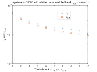
(a)

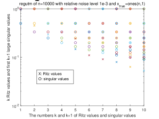
(b)

Fig. 1: (a): The accuracy $\gamma_{k}$ of rank $k$ approximations and the singular values $\sigma_{k}=\frac{1}{k}$; (b) The $k$ Ritz values $\theta_{i}^{(k)}$ and the first $k+1$ large singular values $\sigma_{i}$.

(a)

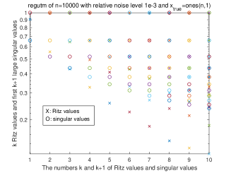
(b)

Fig. 2: (a): The accuracy $\gamma_{k}$ of rank $k$ approximations and the singular values $\sigma_{k}=\frac{1}{k^{0.6}}$; (b) The $k$ Ritz values $\theta_{i}^{(k)}$ and the first $k+1$ large singular values $\sigma_{i}$.

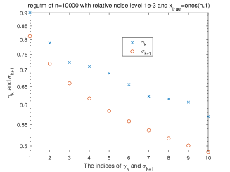
(a)

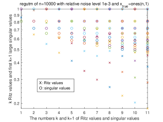
(b)

Fig. 3: (a): The accuracy $\gamma_{k}$ of rank $k$ approximations and the singular values $\sigma_{k}=\frac{1}{k^{0.3}}$; (b) The $k$ Ritz values $\theta_{i}^{(k)}$ and the first $k+1$ large singular values $\sigma_{i}$.

Table 1: The accuracy $\gamma_{k}$ of rank $k$ approximations and the approximation behavior of the Ritz values $\theta_{i}^{(k)},\ i=1,2,\ldots,k$.

$\sigma_{k}=\frac{1}{k},\ k=1,2,\ldots,n$ The location of $\gamma_{k}$ near best $\#<\sigma_{k+1}$ $\#$ attained $\gamma_{5}\in(\sigma_{6},\sigma_{5})$ closer to $\sigma_{6}$ yes 1 yes $\gamma_{6}\in(\sigma_{7},\sigma_{6})$ closer to $\sigma_{7}$ yes 1 yes $\gamma_{7}\in(\sigma_{7},\sigma_{6})$ closer to $\sigma_{6}$ no 1 no $\gamma_{8}\in(\sigma_{8},\sigma_{7})$ closer to $\sigma_{7}$ no 1 no $\gamma_{9}\in(\sigma_{8},\sigma_{7})$ closer to $\sigma_{8}$ no 2 no $\gamma_{10}\in(\sigma_{10},\sigma_{9})$ closer to $\sigma_{10}$ no 2 yes $\sigma_{k}=\frac{1}{k^{0.6}},\ k=1,2,\ldots,n$ The location of $\gamma_{k}$ near best $\#<\sigma_{k+1}$ $\#$ attained $\gamma_{3}\in(\sigma_{4},\sigma_{3})$ closer to $\sigma_{3}$ no 1 no $\gamma_{4}\in(\sigma_{4},\sigma_{3})$ closer to $\sigma_{4}$ no 1 no $\gamma_{5}\in(\sigma_{6},\sigma_{5})$ closer to $\sigma_{5}$ no 1 no $\gamma_{6}\in(\sigma_{6},\sigma_{5})$ closer to $\sigma_{6}$ no 1 no $\gamma_{7}\in(\sigma_{7},\sigma_{6})$ closer to $\sigma_{7}$ no 2 yes $\gamma_{8}\in(\sigma_{7},\sigma_{6})$ closer to $\sigma_{7}$ no 2 no $\gamma_{8}\in(\sigma_{7},\sigma_{6})$ closer to $\sigma_{7}$ no 2 no $\gamma_{9}\in(\sigma_{7},\sigma_{6})$ closer to $\sigma_{7}$ no 2 no $\gamma_{10}\in(\sigma_{8},\sigma_{7})$ closer to $\sigma_{7}$ no 2 no $\sigma_{k}=\frac{1}{k^{0.3}},\ k=1,2,\ldots,n$ The location of $\gamma_{k}$ near best $\#<\sigma_{k+1}$ $\#$ attained $\gamma_{2}\in(\sigma_{3},\sigma_{2})$ closer to $\sigma_{2}$ no 1 yes $\gamma_{3}\in(\sigma_{4},\sigma_{3})$ closer to $\sigma_{3}$ no 1 no $\gamma_{4}\in(\sigma_{4},\sigma_{3})$ closer to $\sigma_{4}$ no 2 yes $\gamma_{5}\in(\sigma_{6},\sigma_{5})$ closer to $\sigma_{4}$ no 2 no $\gamma_{6}\in(\sigma_{5},\sigma_{4})$ closer to $\sigma_{4}$ no 2 no $\gamma_{7}\in(\sigma_{5},\sigma_{4})$ closer to $\sigma_{5}$ no 2 no $\gamma_{8}\in(\sigma_{5},\sigma_{4})$ closer to $\sigma_{5}$ no 3 no $\gamma_{8}\in(\sigma_{5},\sigma_{4})$ closer to $\sigma_{5}$ no 3 no $\gamma_{9}\in(\sigma_{5},\sigma_{4})$ closer to $\sigma_{7}$ no 3 no $\gamma_{10}\in(\sigma_{6},\sigma_{5})$ closer to $\sigma_{6}$ no 4 no

Several comments are made in order on the figures and table.

Firstly, for the test problem with $\alpha=1$, we observe from Figure 1 (a) that $P_{k+1}B_{k}Q_{k}^{T}$ is a near best rank $k$ approximation to $A$ for $k=1,2,\ldots,6$ and afterwards it is not any longer. However, starting from $k=5$ onwards, the $\theta_{i}^{(k)}$ do not approximate the $k$ large singular values $\sigma_{i}$ of $A$ in natural order, as is clearly displayed in Figure 1 (b). This indicates that the near best rank $k$ approximations for $k=5,6$ cannot guarantee that the $\theta_{i}^{(k)}$ approximate the $\sigma_{i}$ in natural order, confirming our theory. Furthermore, it is seen from Table 1 that in each of these two cases there is exactly one Ritz value $\theta_{k}^{(k)}<\sigma_{k+1}$, which coincides with the maximum possible number estimated by Theorem 17.

Secondly, by comparing (a) with (b) in Figures 1–3 correspondingly, we observe that there is always at least one Ritz value $\theta_{k}^{(k)}<\sigma_{k+1}$ whenever $P_{k+1}B_{k}Q_{k}^{T}$ is not a near best rank $k$ approximation to $A$. We have described these features more clearly in Table 1.

Thirdly, by inspecting Figures 1–3 and Table 1, we find that, for the same $k$, the smaller $\alpha$ is, the less accurate the rank $k$ approximation, since for the same $k$ it is clear that $\gamma_{k}$ is further away from $\sigma_{k+1}$, which can be seen from the interval in which $\gamma_{k}$ lies. This justifies that it is harder to generate a good rank $k$ approximation when the decay of the singular values becomes slower. Particularly, the rank $k$ approximations are not near best for $\alpha=0.6$ and $0.3$ from iterations $k=2$ and $k=1$ upwards, respectively.

Fourthly, we observe from Figures 1–2 (b) that the smaller $\alpha$ is, the earlier the Ritz values $\theta_{i}^{(k)}$ fail to approximate the $\sigma_{i}$ in natural order. Precisely, we can see from the figures that such $k$’s are 5, 3 and 2 for $\alpha=1,0.6$ and $0.3$, respectively. Generally, we deduce that the approximations in natural order fail sooner as the decay of the singular values is slower.

Fifthly, for each $\alpha$, we see from Figures 1–3 and Table 1 that as $k$ increases, the rank $k$ approximation generally becomes poorer and the number of $\theta_{i}^{(k)}<\sigma_{k+1}$ exhibits an increasing tendency.

Sixthly, for different $\alpha$, we observe from Table 1 that for the same $k$ and the smaller $\alpha$, the number of $\theta_{i}^{(k)}<\sigma_{k+1},\ i=1,2,\ldots,k$ is at least nondecreasing and often increases.

Seventhly, for each $\alpha$ and given maximum $k=10$ there is always at least one iteration $j\leq k$ at which the number of $\theta_{i}^{(j)}<\sigma_{j+1}$ is exactly equal to its possible maximum; see the fourth column of Table 1.

Next, we report the results on regutm of $m=n=10,000$ with $\sigma_{k}=\frac{1}{k^{2}}$, i.e., $\alpha=2$, $x_{true}=ones(n,1)$ and the relative noise level $\varepsilon=10^{-3}$. This is a moderately ill-posed problem with $\alpha>1$ fairly. We aim to justify Theorems 13–14 and the second part of Theorem 16. Figure 4 (a)-(b) depict the accuracy $\gamma_{k}$ versus $\sigma_{k+1}$ and the $k$ Ritz values $\theta_{i}^{(k)}$ and the first $k+1$ singular values $\sigma_{i},\ k=1,2,\ldots,10$, respectively.

Clearly, we observe from the figure that $P_{k+1}B_{k}Q_{k}^{T}$ is a near best rank $k$ approximation to $A$ until $k=7$ and afterwards it is not any longer. Correspondingly, the $k$ Ritz values $\theta_{i}^{(k)}$ interlace the first $k+1$ large singular values $\sigma_{i}$ until the same $k$. Afterwards, such interlacing property is lost, and the Ritz values do not approximate the singular values in natural order any more. These justify Theorems 13–14, in which, for a fixed $\alpha>1$, the sufficient conditions (74) and (76) fail to meet when $k$ increases up to some point, since the left-hand sides strictly increase and the right-hand sides strictly decrease with $k$ for the fixed $\alpha$. They also confirm the second part of Theorem 16, which requires that $\alpha>1$ sufficiently for a given not small $k$, while $\alpha=2$ cannot meet this requirement for $k>7$.

By comparing Figure 4 with Figures 1–3, we mention that $k=7$ is considerably bigger than those for $\alpha=1,0.6$ and $0.3$, after which $P_{k+1}B_{k}Q_{k}^{T}$ is not a near best rank $k$ approximation and the Ritz values fail to approximate the singular values in natural order. This again confirms that, for the same $k$, the rank $k$ approximation $P_{k+1}B_{k}Q_{k}^{T}$ is more accurate and the Ritz values are more likely to approximate the singular values in natural order for a bigger $\alpha$.

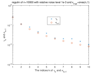
(a)

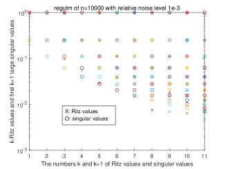
(b)

Fig. 4: (a): The accuracy $\gamma_{k}$ of rank $k$ approximations and the singular values $\sigma_{k}=\frac{1}{k^{2}}$; (b) The $k$ Ritz values $\theta_{i}^{(k)}$ and the first $k+1$ large singular values $\sigma_{i}$.

Finally, we justify Theorem 15 and the first two remarks followed. Figure 5 depicts $\gamma_{k}$ versus $\alpha_{k+1}+\beta_{k+2}$ for regutm with $\alpha=2,1,0.6$ and $0.3$. Clearly, we see from the figure that $\alpha_{k+1}+\beta_{k+2}$ decays exactly as fast as $\gamma_{k}$. Therefore, independent of the degree of ill-posedness, we can reliably judge the decreasing property and tendency of the practically uncomputable accuracy $\gamma_{k}$ by the available $\alpha_{k+1}+\beta_{k+2}$ with little cost. In addition, it is clearly seen from the figure that $\gamma_{k}$ decays faster for a bigger $\alpha$ than for a smaller $\alpha$.

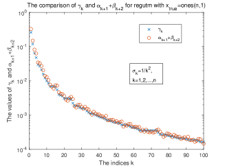
(a)

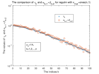
(b)

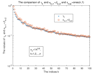
(c)

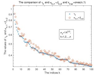
(d)

Fig. 5: $\gamma_{k}$ versus $\alpha_{k+1}+\beta_{k+2}$ for regutm of $m=n=10,000$ with $\alpha=2,1,0.6$ and $0.3$.

9 Conclusions

For the large-scale ill-posed problem (1), LSQR is a most commonly used Krylov solver for general purposes. It has general regularizing effects and exhibits semi-convergence. If LSQR has already found best possible 2-norm filtering regularized solutions, then it has the full regularization. In this case, we simply stop it after a few iterations of semi-convergence, and complicated hybrid variants are not needed. The semi-convergence of LSQR, in principle, can be determined by a suitable parameter-choice method, such as the L-curve criterion and the discrepancy principle [23, 25]

In the simple singular value case, the author in [33, 34] has proved that, for the severely and moderately ill-posed problems with suitable $\rho>1$ and $\alpha>1$, the Ritz values $\theta_{i}^{(k)}$ approximate the large singular values of $A$ in natural order until the semi-convergence, so that LSQR has the full regularization. On the other hand, however, if $\alpha>1$ not enough, the approximation in this order cannot be ensured; if $\alpha\leq 1$, such approximation property may hold only for $k$ very small. In this paper, we have nontrivially extended the results in [33, 34] to the multiple singular value case, and drawn the same conclusions.

As a major contribution, we have made an in-depth analysis on best, near best and general rank $k$ approximations to $A$ for more general ill-posed problems with $\alpha>0$, which include mildly ill-posed problems, and derived some insightful properties of the Ritz values $\theta_{i}^{(k)},\ i=1,2,\ldots,k$. Our results have shown that general best or near best rank $k$ approximations do not guarantee that $\theta_{i}^{(k)},\ i=1,2,\ldots,k$ approximate large singular values of $A$ in natural order for $0<\alpha\leq 1$. We have proved that, for the same $k$, the smaller $\alpha$ is, the less accurate the rank $k$ approximation is, and the more Ritz values smaller than $\sigma_{k+1}$. Numerical experiments have confirmed the theoretical results. These results apply to the other Krylov solvers CGME, MINRES, MR-II, GMRES and RRGMRES as well.

References

[1]
R. C. Aster, B. Borchers, and C. H. Thurber, Parameter Estimation and
Inverse Problems, second ed., Elsevier, New York, 2013.
[2]
S. Berisha and J. G. Nagy, Restore tools: Iterative methods for image
restoration, 2012, available from
http://www.mathcs.emory.edu/∼nagy/RestoreTools.
[3]
Å. Björck, A bidiagonalization algorithm for solving large and
sparse ill-posed systems of linear equations, BIT, (28) (1988), pp. 659–670.
[4]
Å. Björck, Numerical Methods for Least Squares
Problems, SIAM, Philadelphia, PA, 1996.
[5]
Å. Björck, Numerical Methods in Matrix Computations, Texts in
Applied Mathematics, vol. 59, Springer, Cham, 2015.
[6]
Å. Björck and L. Eldén, Methods in numerical algebra for
ill-posed problems, Report LiTH-R-33-1979, Dept. of Mathematics,
Linköping Univeristy, Sweden, 1979.
[7]
Å. Björck, E. Grimme, and P. van Dooren, An implicit shift
bidiagonalization algorithm for ill-posed systems, BIT Numer. Math.,
34 (1994), pp. 510–534.
[8]
J. Chung, J. G. Nagy, and D. P. O’Leary, A weighted-GCV method for
Lanczos-hybrid regularization, Electr. Trans. Numer. Anal., 28
(2007/08), pp. 149–167.
[9]
J. Chung and K. Palmer, A hybrid LSMR algorithm for large-scale
Tikhonov regularization, SIAM J. Sci. Comput., 37 (2015),
pp. S562–S580.
[10]
E. J. Craig, The -step iteration procedures, J. Math. Phys.,
34 (1955), pp. 64–73.
[11]
H. W. Engl, Regularization methods for the stable solution of inverse
problems, Surveys Math. Indust., 3 (1993), pp. 71–143.
[12]
H. W. Engl, M. Hanke, and A. Neubauer, Regularization of Inverse
Problems, Kluwer Academic Publishers, 2000.
[13]
R. D. Fierro, G. H. Golub, P. C. Hansen, and D. P. O’Leary,
Regularization by truncated total least squares, SIAM J. Sci. Comput.,
18 (1997), pp. 1223–1241.
[14]
D. C. L. Fong and M. Saunders, LSMR: an iterative algorithm for sparse
least-squares problems, SIAM J. Sci. Comput., 33 (2011), pp. 2950–2971.
[15]
S. Gazzola, P. C. Hansen, and J. G. Nagy, IR tools: A MATLAB package
of iterative regularization methods and large-scale test problems, Numer.
Algor., 81 (2019), pp. 773–811.
[16]
S. Gazzola and P. Novati, Inheritance of the discrete Picard condition
in Krylov subspace methods, BIT Numer. Math., 56 (2016), pp. 893–918.
[17]
S. F. Gilyazov and N. L. Gol’dman, Regularization of Ill-Posed
Problems by Iteration Methods, Mathematics and its Applications, vol.
499, Kluwer Academic Publishers, Dordrecht, 2000.
[18]
M. Hanke, Conjugate gradient Type Methods for Ill-Posed
Problems, Pitman Research Notes in Mathematics Series, vol. 327, Longman,
Essex, 1995.
[19]
M. Hanke, On Lanczos based methods for the regularization of discrete
ill-posed problems, BIT Numer. Math., 41 (2001), Suppl.,
1008–1018.
[20]
M. Hanke and P. C. Hansen, Regularization methods for large-scale
problems, Surveys Math. Indust. 3 (1993), no. 4, 253–315.
[21]
M. Hanke and J. G. Nagy, Restoration of atmospherically blurred images by
symmetric indefinite conjugate gradient techniques, Inverse Probl.,
12 (1996), pp. 157–173.
[22]
P. C. Hansen, Truncated singular value decomposition solutions to
discrete ill-posed problems with ill-determined numerical rank, SIAM J. Sci.
Statist. Comput., 11 (1990), pp. 503–518.
[23]
P. C. Hansen, Rank-Deficient and Discrete Ill-Posed Problems:
Numerical Aspects of Linear Inversion, SIAM Monographs on
Mathematical Modeling and Computation, SIAM, Philadelphia, PA, 1998.
[24]
P. C. Hansen, Regularization Tools version 4.0 for Matlab 7.3, Numer.
Algor., 46 (2007), pp. 189–194.
[25]
P. C. Hansen, Discrete Inverse Problems: Insight and Algorithms,
SIAM, Philadelphia, PA, 2010.
[26]
M. R. Hestenes and E. Stiefel, Methods of conjugate gradients for solving
linear systems, J. Res. Nat. Bur. Stand., 49 (1952), pp. 409–436.
[27]
M. R. Hnětynková, Marie Kubínová, and M. Plešinger,
Noise representation in residuals of LSQR, LSMR, and Craig
regularization, Linear Algebra Appl., 533 (2017), pp. 357–379.
[28]
M. R. Hnětynková, M. Plešinger, and Z. Strakoš, The
regularizing effect of the Golub-Kahan iterative bidiagonalization and
revealing the noise level in the data, BIT Numer. Math., 49 (2009),
pp. 669–696.
[29]
B. Hofmann, Regularization for Applied Inverse and Ill-Posed
Problems, Teubner, Stuttgart, Germany, 1986.
[30]
Y. Huang and Z. Jia, On regularizing effects of MINRES and MR-II for
large-scale symmetric discrete ill-posed problems, J. Comput. Appl. Math.,
320 (2017), pp. 145–163.
[31]
Y. Huang and Z. Jia, Some results on the regularization of LSQR for large-scale
ill-posed problems, Science China Math., 60 (2017), pp. 701–718.
[32]
T. K. Jensen and P. C. Hansen, Iterative regularization with
minimum-residual methods, BIT Numer. Math., 47 (2007), PP. 103–120.
[33]
Z. Jia, Approximation accuracy of the Krylov subspaces for linear
discrete ill-posed problems, J. Comput. Appl. Math. (2020),
https://doi.org/10.1016/j.cam.2020.112786
[34]
Z. Jia, The low rank approximations and Ritz values in LSQR for
linear discrete ill-posed problems, Inverse Probl. (2020),
https://doi.org/10.1088/1361-6420/ab6f42.
[35]
Z. Jia, Regularization properties of the Krylov iterative solvers
CGME and LSMR for linear discrete ill-posed problems with an application
to truncated randomized SVDs, Numer. Algor. (2020),
https://dx.doi.org/10.1007/s11075-019-00865-w.
[36]
J. Kaipio and E. Somersalo, Statistical and Computational Inverse
Problems, Springer-Verlag, New
York, 2005.
[37]
M. Kern, Numerical Methods for Inverse Problems, John Wiley &
Sons, Inc., 2016.
[38]
M. E. Kilmer and G. W. Stewart, Iterative regularization and MINRES,
SIAM J. Matrix Anal. Appl., 21 (1999), pp. 613–628.
[39]
A. Kirsch, An Introduction to the Mathematical Theory of Inverse
Problems, second ed., Springer,
New York, 2011.
[40]
J. L. Mueller and S. Siltanen, Linear and Nonlinear Inverse
Problems with Practical Applications,
SIAM, Philadelphia, PA, 2012.
[41]
F. Natterer, The Mathematics of Computerized Tomography,
SIAM, Philadelphia, PA, 2001, Reprint of the 1986 original edition.
[42]
G. Nolet, Solving or resolving inadequate and noisy tomographic systems,
J. Comput. Phys., 61 (1985), pp. 463–482.
[43]
D. P. O’Leary and J. A. Simmons, A bidiagonalization-regularization
procedure for large scale discretizations of ill-posed problems, SIAM J.
Sci. Statist. Comput., 2 (1981), pp. 474–489.
[44]
C. C. Paige and M. A. Saunders, LSQR: an algorithm for sparse linear
equations and sparse least squares, ACM Trans. Math. Software, 8
(1982), pp. 43–71.
[45]
C. C. Paige and Z. Z. Strakoš, Core problems in linear algebraic
systems, SIAM J. Matrix Anal. Appl., 27 (2005), pp. 861–875.
[46]
R. A. Renaut, S. Vatankhah, and V. E. Ardestani, Hybrid and iteratively
reweighted regularization by unbiased predictive risk and weighted GCV,
SIAM J. Sci. Comput., 39 (2017), pp. B221–B243.
[47]
J. A. Scales and A. Gerztenkorn, Robust methods in inverse theory,
Inverse Probl., 4 (1988), pp. 1071–1091.
[48]
G. W. Stewart, Matrix Algorithms II: Eigensystems, SIAM,
Philadelphia, PA, 2001.
[49]
G. W. Stewart and J.-G Sun, Matrix Perturbation Theory, Computer
Science and Scientific Computing, Academic Press, Inc., Boston, MA, 1990.
[50]
A. van der Sluis and H. A. van der Vorst, The rate of convergence of
conjugate gradients, Numer. Math., 48 (1986), pp. 543–560.
[51]
J. M. Varah, A practical examination of some numerical methods for linear
discrete ill-posed problems, SIAM Rev., 21 (1979), pp. 100–111.
[52]
C. R. Vogel, Computational Methods for Inverse Problems,
SIAM, Philadelphia, PA, 2002.