Environment-assisted bosonic quantum communications

Abstract

We consider a quantum relay which is used by two parties to perform several continuous-variable protocols of quantum communication, from entanglement distribution (swapping and distillation), to quantum teleportation, and quantum key distribution. The theory of these protocols is suitably extended to a non-Markovian model of decoherence characterized by correlated Gaussian noise in the bosonic environment. In the worst case scenario where bipartite entanglement is completely lost at the relay, we show that the various protocols can be reactivated by the assistance of classical (separable) correlations in the environment. In fact, above a critical amount, these correlations are able to guarantee the distribution of a weaker form of entanglement (quadripartite), which can be localized by the relay into a stronger form (bipartite) that is exploitable by the parties. Our findings are confirmed by a proof-of-principle experiment where we show, for the first time, that memory effects in the environment can drastically enhance the performance of a quantum relay, well beyond the single-repeater bound for quantum and private communications.

The concept of a relay is at the basis of network information theory CoverThomas . Indeed the simplest network topology is composed by three nodes: two end-users, Alice and Bob, plus a third party, the relay, which assists their communication. This scenario is inherited by quantum information theory book1 ; book2 ; book3 ; book4 ; book5 ; book6 ; book7 ; book8 ; RMP ; RMP2 ; hybrid1 ; hybrid2 , where the mediation of a quantum relay can be found in a series of fundamental protocols. By sending quantum systems to a middle relay, Alice and Bob may perform entanglement swapping Zukowski ; EntSwap ; EntSwap2 ; GaussSWAP , entanglement distillation Briegel , quantum teleportation Tele ; Tele2 ; telereview and quantum key distribution (QKD) mdiQKD ; Lo ; Untrusted ; TFQKD ; SNSwang ; QKDrev .

Quantum relays are crucial elements for quantum network architectures at any scale, from short-range implementations on quantum chips to long-distance quantum communication. In all cases, their working mechanism has been studied assuming Markovian decoherence models, where the errors are independent and identically distributed (iid). Removing this iid approximation is one of the goals of modern quantum information theory.

In a quantum chip (e.g., photonic photonic1 ; photonic2 or superconducting chip3 ), quantum relays can distribute entanglement among registers and teleport quantum gates. Miniaturizing this architecture, correlated errors may come from unwanted interactions between quantum systems. A common bath may be introduced by a variety of imperfections, e.g., due to diffraction, slow electronics etc. It is important to realize that non-Markovian dynamics Petruccione will become increasingly important as the size of quantum chips further shrinks.

At long distances (in free-space or fibre), quantum relays intervene to assist quantum communication, entanglement and key distribution. Here, noise-correlations and memory effects may naturally arise when optical modes are employed in high-speed communications UlrikCORR , or propagate through atmospheric turbulence Tyler09 ; Semenov09 ; Boyd11 and diffraction-limited linear systems. Most importantly, correlated errors must be considered in relay-based QKD, where an eavesdropper (Eve) may jointly attack the two links with the relay (random permutations and de Finetti arguments Renner1 ; Renner2 cannot remove these residual correlations). Eve can manipulate the relay itself as assumed in measurement-device independent QKD mdiQKD ; Lo ; Untrusted . Furthermore, Alice’s and Bob’s setups may also be subject to correlated side-channel attacks.

For all these reasons, we generalize the study of quantum relays to non-Markovian conditions, developing the theory for continuous variable (CV) systems RMP (qubits are discussed in the Supplemental Material). We consider an environment whose Gaussian noise may be correlated between the two links. Our model is formulated as a spatial non-Markovian model, where spatially-separated bosonic modes are subject to correlated errors, but could also be connected to a time-like model where the parties use the same channel at different times. In this scenario, while the relay always performs the same measurement, the parties may implement different protocols (swapping, distillation, teleportation, or QKD) all based, directly or indirectly, on the exploitation of bipartite entanglement.

We find a surprising behavior in conditions of extreme decoherence. We consider entanglement-breaking links EBchannels ; HolevoEB , so that no protocol can work under Markovian conditions. We then induce non-Markovian effects by progressively increasing the noise correlations in the environment while keeping their nature separable (so that there is no external reservoir of entanglement). While these correlations are not able to re-establish bipartite entanglement (or tripartite entanglement) we find that a critical amount reactivates quadripartite entanglement, between the setups and the modes transmitted. In other words, by increasing the separable correlations above a ‘reactivation threshold’ we can retrieve the otherwise lost quadripartite entanglement (it is in this sense that we talk of ‘reactivated’ entanglement below). The measurement of the relay can then localize this multipartite entanglement into a bipartite form, shared by the two remote parties and exploitable for the various protocols.

As a matter of fact, we find that all the quantum protocols can be reactivated. In particular, their reactivation occurs in a progressive fashion, so that increasing the environmental correlations first reactivates entanglement swapping and teleportation, then entanglement distillation and finally QKD. Our theory is confirmed by a proof-of-principle experiment which shows the reactivation of the most nested protocol, i.e., the QKD protocol. In particular, we show that the key rate of this environmental-assisted protocol outperforms the single-repeater upper-bound for private communication RepBound , i.e., the maximum secret key rate that is achievable in the presence of memory-less links.

Results

General scenario.– As depicted in Fig. 1, we consider two parties, Alice and Bob, whose devices are connected to a quantum relay, Charlie, with the aim of implementing a CV protocol (swapping, distillation, teleportation, or QKD). The connection is established by sending two modes, $A$ and $B$, through a joint quantum channel $\mathcal{E}_{AB}$, whose outputs $A^{\prime}$ and $B^{\prime}$ are subject to a CV Bell detection BellFORMULA . This means that modes $A^{\prime}$ and $B^{\prime}$ are mixed at a balanced beam splitter and then homodyned, one in the position quadrature $\hat{q}_{-}=(\hat{q}_{A^{\prime}}-\hat{q}_{B^{\prime}})/\sqrt{2}$ and the other in the momentum quadrature $\hat{p}_{+}=(\hat{p}_{A^{\prime}}+\hat{p}_{B^{\prime}})/\sqrt{2}$. The classical outcomes $q_{-}$ and $p_{+}$ can be combined into a complex variable $\gamma:=q_{-}+ip_{+}$, which is broadcast to Alice and Bob through a classical public channel.

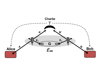
Figure 1: Quantum relay. Alice and Bob connect their devices (red boxes) to a quantum relay, Charlie, for implementing a CV protocol. On the received modes, Charlie always performs a CV Bell detection whose outcome $\gamma$ is broadcast. Separable Gaussian environment. The travelling modes are subject to a joint Gaussian channel $\mathcal{E}_{AB}$. This is realized by two beam splitters with tranmissivity $\tau$ which mix $A$ and $B$ with two ancillary modes, $E_{1}$ and $E_{2}$, respectively. These ancillas inject thermal noise with variance $\omega$ and belong to a correlated (but separable) Gaussian state $\rho_{E_{1}E_{2}}$. Entanglement breaking. For $\omega>\omega_{\text{EB}}(\tau)$, bipartite (and tripartite) entanglement cannot survive at the relay. In particular, $A^{\prime}$ is disentangled from Alice’s device, and $B^{\prime}$ is disentangled from Bob’s, no matter if the environment is correlated or not. Non-Markovian reactivation. Above a critical amount of separable correlations, quadripartite entanglement is reactivated between Alice’s and Bob’s devices and the transmitted modes, $A^{\prime}$ and $B^{\prime}$. Bell detection can localize this multipartite resource into a bipartite form and reactivate all the protocols.

The joint quantum channel $\mathcal{E}_{AB}$ corresponds to an environment with correlated Gaussian noise. This is modelled by two beam splitters (with transmissivity $0<\tau<1$) mixing modes $A$ and $B$ with two ancillary modes, $E_{1}$ and $E_{2}$, respectively (see Fig. 1). These ancillas are taken in a zero-mean Gaussian state RMP $\rho_{E_{1}E_{2}}$ with covariance matrix (CM) in the symmetric normal form

$$\mathbf{V}_{E_{1}E_{2}}(\omega,g,g^{\prime})=\left(\begin{array}[c]{cc}\omega\mathbf{I}&\mathbf{G}\\ \mathbf{G}&\omega\mathbf{I}\end{array}\right),~{}\begin{array}[c]{c}\mathbf{I}:=\mathrm{diag}(1,1),\\ \mathbf{G}:=\mathrm{diag}(g,g^{\prime}).\end{array}$$

Here $\omega\geq 1$ is the variance of local thermal noise, while the block $\mathbf{G}$ accounts for noise-correlations.

For $\mathbf{G}=\mathbf{0}$ we retrieve the standard Markovian case, based on two independent lossy channels EntSwap ; EntSwap2 ; GaussSWAP . For $\mathbf{G}\neq\mathbf{0}$, the lossy channels become correlated, and the local dynamics cannot reproduce the global non-Markovian evolution of the system. Such a separation becomes more evident by increasing the correlation parameters, $g$ and $g^{\prime}$, whose values are bounded by the bona-fide conditions $|g|<\omega$, $|g^{\prime}|<\omega$, and $\omega\left|g+g^{\prime}\right|\leq\omega^{2}+gg^{\prime}-1$ TwomodePRA ; NJPpirs . In particular, we consider the realistic case of separable environments ($\rho_{E_{1}E_{2}}$ separable), identified by the additional constraint $\omega\left|g-g^{\prime}\right|\leq\omega^{2}-gg^{\prime}-1$ NJPpirs . The amount of separable correlations can be quantified by the quantum mutual information $I(g,g^{\prime})$.

To analyse entanglement breaking, assume the asymptotic infinite-energy scenario where Alice’s (Bob’s) device has a remote mode $a$ ($b$) which is maximally entangled with $A$ ($B$). We then study the separability properties of the global system composed by $a$, $b$, $A^{\prime}$ and $B^{\prime}$. In the Markovian case ($\mathbf{G}=\mathbf{0}$), all forms of entanglement (bipartite, tripartite tripartite , and quadripartite quadripartite ) are absent for $\omega>\omega_{\text{EB}}(\tau):=(1+\tau)/(1-\tau)$, so that no protocol can work. In the non-Markovian case ($\mathbf{G}\neq\mathbf{0}$) the presence of separable correlations does not restore bipartite or tripartite entanglement when $\omega>\omega_{\text{EB}}(\tau)$. However, a sufficient amount of these correlations is able to reactivate $1\times 3$ quadripartite entanglement quadripartite , in particular, between mode $a$ and the set of modes $bA^{\prime}B^{\prime}$. See Fig. 9.

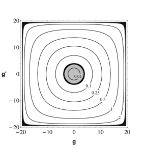
Figure 2: Non-Markovian reactivation of $1\times 3$ quadripartite entanglement. Assuming maximally-entangled states for the parties, and entanglement-breaking conditions (here $\tau=0.9$ and $\omega=1.02\times\omega_{\text{EB}}=19.38$), we show how quadripartite entanglement is reactivated by increasing the separable correlations of the environment (bits of quantum mutual information, which are constant over the concentric contour lines). Inside the gray region there is no quadripartite entanglement with respect to any $1\times 3$ grouping of the four modes $abA^{\prime}B^{\prime}$. Outside the gray region all the possible $1\times 3$ groupings are entangled. The external black region is excluded, as it corresponds to entangled or unphysical environments.

Once quadripartite entanglement is available, the Bell detection on modes $A^{\prime}$ and $B^{\prime}$ can localize it into a bipartite form for modes $a$ and $b$. For this reason, entanglement swapping and the other protocols can be reactivated by sufficiently-strong separable correlations. In the following, we discuss these results in detail for each specific protocol, starting from the basic scheme of entanglement swapping. For each protocol, we first generalize the theory to non-Markovian decoherence, showing how the various performances are connected. Then, we analyze the protocols under entanglement breaking conditions.

Entanglement swapping.– The standard source of Gaussian entanglement is the two-mode squeezed vacuum (TMSV) state, which is a realistic finite-energy version of the ideal EPR state RMP . More precisely, this is a two-mode Gaussian state with zero mean-value and CM

$$\mathbf{V}(\mu)=\left(\begin{array}[c]{cc}\mu\mathbf{I}&\sqrt{\mu^{2}-1}\mathbf{Z}\\ \sqrt{\mu^{2}-1}\mathbf{Z}&\mu\mathbf{I}\end{array}\right),~{}\mathbf{Z}:=\mathrm{diag}(1,-1),$$

where the variance $\mu\geq 1$ quantifies its entanglement. Indeed the log-negativity logNEG ; logNEG1 ; logNEG2 is strictly increasing in $\mu$: It is zero for $\mu=1$ and tends to infinity for large $\mu$.

Suppose that Alice and Bob have two identical TMSV states, $\rho_{aA}(\mu)$ describing Alice’s modes $a$ and $A$, and $\rho_{bB}(\mu)$ describing Bob’s modes $b$ and $B$, as in Fig. 3(i). They keep $a$ and $b$, while sending $A$ and $B$ to Charlie through the joint channel $\mathcal{E}_{AB}$ of the Gaussian environment. After the broadcast of the outcome $\gamma$, the remote modes $a$ and $b$ are projected into a conditional Gaussian state $\rho_{ab|\gamma}$, with mean-value $\mathbf{x}=\mathbf{x}(\gamma)$ and conditional CM $\mathbf{V}_{ab|\gamma}$. In the Supplemental Material, we compute

$$\mathbf{V}_{ab|\gamma}=\left(\begin{array}[c]{cc}\mathbf{A}&\mathbf{C}\\ \mathbf{C}^{T}&\mathbf{B}\end{array}\right),$$ (1)

where the $2\times 2$ blocks are given by

$$\mathbf{A} =\mathbf{B}=\mathrm{diag}\left[\mu-\frac{\mu^{2}-1}{2(\mu+\kappa)},\mu-\frac{\mu^{2}-1}{2(\mu+\kappa^{\prime})}\right],$$ (2)

$$\mathbf{C} =\mathrm{diag}\left[\frac{\mu^{2}-1}{2(\mu+\kappa)},-\frac{\mu^{2}-1}{2(\mu+\kappa^{\prime})}\right],$$ (3)

and the $\kappa$’s contain all the environmental parameters

$$\kappa:=(\tau^{-1}-1)(\omega-g),~{}\kappa^{\prime}:=(\tau^{-1}-1)(\omega+g^{\prime}).$$ (4)

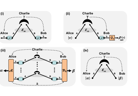
Figure 3: Relay-based quantum protocols in a correlated Gaussian environment. (i) Entanglement swapping. Alice and Bob possess two TMSV states with variance $\mu$. Modes $A$ and $B$ are sent through the joint channel $\mathcal{E}_{AB}$ and received by Charlie. After the outcome $\gamma$ is broadcast, the remote modes, $a$ and $b$, are projected into a conditional state $\rho_{ab|\gamma}$. (ii) Quantum teleportation. Alice’s coherent state $\left|\nu\right\rangle$ is teleported into Bob’s state $\rho_{\text{out}}(\nu)$, after the communication of $\gamma$ and the action of a conditional quantum operation $\mathcal{Q}_{\gamma}$. (iii) Entanglement/key distillation. In the limit of many uses of the relay, Alice performs a quantum instrument on her modes $a$, communicating a classical variable $k$ to Bob, who performs a conditional quantum operation on his modes $b$. This is a non-Gaussian quantum repeater where entanglement swapping is followed by optimal one-way distillation. (iv) Practical QKD. Alice and Bob prepare Gaussian-modulated coherent states to be sent to Charlie. The communication of the outcome $\gamma$ creates remote classical correlations which are used to extract a secret key. Here the role of Charlie could be played by Eve, so that the relay becomes an MDI-QKD node.

From $\mathbf{V}_{ab|\gamma}$ we compute the log-negativity $\mathcal{N}=\max\{0,-\log_{2}\varepsilon\}$ of the swapped state, in terms of the smallest partially-transposed symplectic eigenvalue $\varepsilon$ RMP . In the Supplemental Material, we derive

$$\varepsilon=\left[\frac{(1+\mu\kappa)(1+\mu\kappa^{\prime})}{(\mu+\kappa)(\mu+\kappa^{\prime})}\right]^{1/2}.$$ (5)

For any input entanglement ($\mu>1$), swapping is successful ($\varepsilon<1$) whenever the environment has enough correlations to satisfy the condition $\kappa\kappa^{\prime}<1$. The actual amount of swapped entanglement $\mathcal{N}$ increases in $\mu$, reaching its asymptotic optimum for large $\mu$, where

$$\varepsilon\simeq\varepsilon_{\text{opt}}:=\sqrt{\kappa\kappa^{\prime}}.$$

Quantum teleportation.– As depicted in Fig. 3(ii), we consider Charlie acting as a teleporter of a coherent state $\left|\nu\right\rangle$ from Alice to Bob. Alice’s state and part of Bob’s TMSV state are transmitted to Charlie through the joint channel $\mathcal{E}_{AB}$. After detection, the outcome $\gamma$ is communicated to Bob, who performs a conditional quantum operation book1 $\mathcal{Q}_{\gamma}$ on mode $b$ to retrieve the teleported state $\rho_{\text{out}}(\nu)\simeq\left|\nu\right\rangle\left\langle\nu\right|$. In the Supplemental Material, we find a formula for the teleportation fidelity $F=F(\mu,\kappa,\kappa^{\prime})$, which becomes asymptotically optimal for large $\mu$, where

$$F\simeq F_{\text{opt}}:=\left[(1+\kappa)(1+\kappa^{\prime})\right]^{-1/2}\leq(1+\varepsilon_{\text{opt}})^{-1}.$$ (6)

Thus, there is a direct connection between the asymptotic protocols of teleportation and swapping: If swapping fails ($\varepsilon_{\text{opt}}\geq 1$), teleportation is classical ($F_{\text{opt}}\leq 1/2$ RMP ). We retrieve the relation $F_{\text{opt}}=(1+\varepsilon_{\text{opt}})^{-1}$ in environments with antisymmetric correlations $g+g^{\prime}=0$.

Entanglement distillation.– Entanglement distillation can be operated on top of entanglement swapping as depicted in Fig. 3(iii). After the parties have run the swapping protocol many times and stored their remote modes in quantum memories, they can perform a one-way entanglement distillation protocol on the whole set of swapped states $\rho_{ab|\gamma}$. This consists of Alice locally applying an optimal quantum instrument Qinstrument $\mathcal{A}$ on her modes $a$, whose quantum outcome $\boldsymbol{\alpha}$ is a distilled system while the classical outcome $k$ is communicated. Upon receipt of $k$, Bob performs a conditional quantum operation $\mathcal{B}_{k}$ transforming his modes $b$ into a distilled system $\boldsymbol{\beta}$.

The process can be designed in such a way that the distilled systems are collapsed into entanglement bits (ebits), i.e., Bell state pairs book1 . The optimal distillation rate (ebits per relay use) is lower-bounded Qinstrument by the coherent information $I_{\mathcal{C}}$ CohINFO ; CohINFO2 computed on the single copy state $\rho_{ab|\gamma}$. In the Supplemental Material, we find a closed expression $I_{\mathcal{C}}=I_{\mathcal{C}}(\mu,\kappa,\kappa^{\prime})$ which is maximized for large $\mu$, where $I_{\mathcal{C}}\simeq-\log_{2}(e\varepsilon_{\text{opt}})$. Asymptotically, entanglement can be distilled for $\varepsilon_{\text{opt}}<e^{-1}\simeq 0.367$.

Secret key distillation.– The scheme of Fig. 3(iii) can be modified into a key distillation protocol, where Charlie (or Eve mdiQKD ) distributes secret correlations to Alice and Bob, while the environment is the effect of a Gaussian attack. Alice’s quantum instrument is here a measurement with classical outputs $\boldsymbol{\alpha}$ (the secret key) and $k$ (data for Bob). Bob’s operation is a measurement conditioned on $k$, which provides the classical output $\boldsymbol{\beta}$ (key estimate). This is an ideal key-distribution protocol KeyCAP whose rate is lower-bounded by the coherent information, i.e., $K\geq I_{\mathcal{C}}$ (see Supplemental Material).

Practical QKD.– The previous key-distribution protocol can be simplified by removing quantum memories and using single-mode measurements, in particular, heterodyne detections. This is equivalent to a run-by-run preparation of coherent states, $\left|\alpha\right\rangle$ on Alice’s mode $A$, and $\left|\beta\right\rangle$ on Bob’s mode $B$, whose amplitudes are Gaussianly modulated with variance $\mu-1$. As shown in Fig. 3(iv), these states are transmitted to Charlie (or Eve mdiQKD ) who measures and broadcasts $\gamma\simeq\alpha-\beta^{\ast}$.

Assuming ideal reconciliation RMP , the secret key rate $R=R(\mu,\kappa,\kappa^{\prime})$ increases in $\mu$. Modulation variances $\mu\gtrsim 50$ are experimentally achievable and well approximate the asymptotic limit for $\mu\gg 1$, where the key rate is optimal and satisfies (see Supplemental Material)

$$R_{\text{opt}}\gtrsim\log_{2}\left(\frac{F_{\text{opt}}}{e^{2}\varepsilon_{\text{opt}}}\right)+h(1+2\varepsilon_{\text{opt}}),$$ (7)

with $h(x):=\frac{x+1}{2}\log_{2}\frac{x+1}{2}-\frac{x-1}{2}\log_{2}\frac{x-1}{2}$. Using Eq. (6), we see that the right hand side of Eq. (7) can be positive only for $\varepsilon_{\text{opt}}\lesssim 0.192$. Thus the practical QKD protocol is the most difficult to reactivate: Its reactivation implies that of entanglement/key distillation and that of entanglement swapping. This is true not only asymptotically but also at finite $\mu$ as we show below.

Reactivation from entanglement breaking.– Once the theory of the previous protocols has been extended to non-Markovian decoherence, we can study their reactivation from entanglement breaking conditions. Consider an environment with transmissivity $\tau$ and entanglement-breaking thermal noise $\omega>\omega_{\text{EB}}(\tau)$, so that no protocol can work for $\mathbf{G}=\mathbf{0}$. By increasing the separable correlations in the environment, not only can quadripartite entanglement be reactivated but, above a certain threshold, it can also be localized into a bipartite form by the relay’s Bell detection. Once entanglement swapping is reactivated, all other protocols can progressively be reactivated. As shown in Fig. 4, there are regions of the correlation plane where entanglement can be swapped ($\mathcal{N}>0$), teleportation is quantum ($F>1/2$), entanglement and keys can be distilled ($I_{\mathcal{C}}$, $K>0$), and practical QKD can be performed ($R>0$). This occurs both for large and experimentally-achievable values of $\mu$.

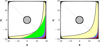
Figure 4: Non-Markovian reactivation of quantum protocols from entanglement-breaking (here $\tau=0.9$ and $\omega=1.02\times\omega_{\text{EB}}=19.38$). Each point of the correlation plane corresponds to a Gaussian environment with separable correlations. In panel a we consider the optimal scenario of large $\mu$ (asymptotic protocols). Once quadripartite $1\times 3$ entanglement has been reactivated (outside the gray ring), we have the progressive reactivation of entanglement swapping ($\mathcal{N}>0$, yellow region), quantum teleportation of coherent states ($F>1/2$, green region), entanglement/key distillation ($I_{\mathcal{C}}$, $K>0$, blue region) and practical QKD ($R>0$, red region). Panel b as in a but refers to a realistic scenario with experimentally achievable values of $\mu$. We consider $\mu\simeq 6.5$ TopENT ; TobiasSqueezing as input entanglement for the entanglement-based protocols, and $\mu\simeq 50$ as modulation for the practical QKD protocol. The reactivation phenomenon persists and can be explored with current technology. Apart from teleportation, the other thresholds undergo small modifications.

Note that the reactivation is asymmetric in the plane only because of the specific Bell detection adopted, which generates correlations of the type $g>0$ and $g^{\prime}<0$. Using another Bell detection (projecting onto $\hat{q}_{+}$ and $\hat{p}_{-}$), the performances would be inverted with respect to the origin of the plane. Furthermore, the entanglement localization (i.e., the reactivation of entanglement swapping) is triggered for correlations higher than those required for restoring quadripartite entanglement, suggesting that there might exist a better quantum measurement for this task. The performances of the various protocols improve by increasing the separable correlations of the environment, with the fastest reactivation being achieved along the diagonal $g+g^{\prime}=0$, where swapping and teleportation are first recovered, then entanglement/key distillation and practical QKD, which is the most nested region.

Correlated additive noise.– The phenomenon can also be found in other types of non-Markovian Gaussian environments. Consider the limit for $\tau\rightarrow 1$ and $\omega\rightarrow+\infty$, while keeping constant $n:=(1-\tau)\omega$, $c:=g(\omega-1)^{-1}$ and $c^{\prime}:=g^{\prime}(\omega-1)^{-1}$. This is an asymptotic environment which adds correlated classical noise to modes $A$ and $B$, so that their quadratures undergo the transformations

$$\left(\hat{q}_{A},\hat{p}_{A},\hat{q}_{B},\hat{p}_{B}\right)\rightarrow\left(\hat{q}_{A},\hat{p}_{A},\hat{q}_{B},\hat{p}_{B}\right)+(\xi_{1},\xi_{2},\xi_{3},\xi_{4}).$$

Here the $\xi_{i}$’s are zero-mean Gaussian variables whose covariances $\left\langle\xi_{i}\xi_{j}\right\rangle$ are specified by the classical CM

$$\mathbf{V}\left(n,c,c^{\prime}\right)=n\left(\begin{array}[c]{cc}\mathbf{I}&\mathrm{diag}(c,c^{\prime})\\ \mathrm{diag}(c,c^{\prime})&\mathbf{I}\end{array}\right),$$ (8)

where $n\geq 0$ is the variance of the additive noise, and $-1\leq c,c^{\prime}\leq 1$ quantify the classical correlations. The entanglement-breaking condition becomes $n>2$.

To show non-Markovian effects, we consider the protocol which is the most difficult to reactivate, the practical QKD protocol. We can specify its key rate $R(\mu,n,c,c^{\prime})$ for $c=c^{\prime}=1$ and assume a realistic modulation $\mu\simeq 52$. We then plot $R$ as a function of the additive noise $n$ in Fig. 5. As we can see, the rate decreases in $n$ but remains positive in the region $2<n\leq 4$ where the links with the relay become entanglement-breaking. As we show below, this behaviour persists in the presence of loss, as typically introduced by experimental imperfections.

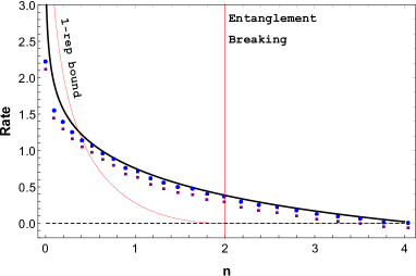
Figure 5: Plot the secret-key rate $R$ (bits per relay use) as a function of the additive noise $n$. The solid black curve is the theoretical rate computed for a correlated-additive environment ($c=c^{\prime}=1$) and realistic signal modulation ($\mu\simeq 52$). This rate is positive after entanglement breaking ($n>2$) and beats the single-repeater bound RepBound (based on memoryless links). Points are experimental data: Blue circles refer to ideal reconciliation, and purple squares to achievable reconcilation efficiency ($\simeq 0.97$). Error bars on the $x$-axis are smaller than the point size. Due to loss at the untrusted relay, the experimental key rate is slightly below the theoretical curve (associated with the correlated side-channel attack).

Recall that, for an additive Gaussian channel with added noise $n$, the secret key capacity (and any other two-way assisted quantum capacity) is upper-bounded by

$$\Phi(n):=\frac{(n/2)-1}{\ln 2}-\log_{2}(n/2),$$ (9)

for $n\leq 2$ and zero otherwise. The bound $\Phi(n)$ in Eq. (9) has been proven in Ref. (PLOB, , Eq. (29)) and here reported in our different vacuum units. In the presence of a relay/repeater, where each link is described by an independent bosonic Gaussian channel, Ref. RepBound established that the secret key capacity assisted by the repeater $K_{\text{1-rep}}$ is upper-bounded by the minimum secret key capacity of the links. In the present setting, we therefore have the single-repeater bound $K_{\text{1-rep}}\leq\Phi(n)$. As we show in Fig. 5, the presence of classical (separable) correlations in the Gaussian environment lead to the violation of the bound $\Phi(n)$ when $n\gtrsim 0.369$ (for the theoretical curve) and $n\gtrsim 0.4$ (for the experimental results).

Experimental results.– Our theoretical results are confirmed by a proof-of-principle experiment, whose setup is schematically depicted in Fig. 6. We consider Alice and Bob generating Gaussianly modulated coherent states by means of independent electro-optical modulators, applied to a common local oscillator. Simultaneously, the modulators are subject to a side-channel attack: Additional electrical inputs are introduced by Eve, whose effect is to generate additional and unknown phase-space displacements. In particular, Eve’s electrical inputs are correlated so that the resulting optical displacements introduce a correlated-additive Gaussian environment described by Eq. (8) with $c\simeq 1$ and $c^{\prime}\simeq 1$. The optical modes then reach the midway relay, where they are mixed at a balanced beam splitter and the output ports photo-detected. Although the measurement is highly efficient, it introduces a small loss ($\simeq 2\%$) which is assumed to be exploited by Eve in the worst-case scenario.

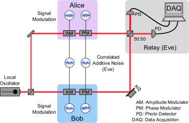
Figure 6: Experimental setup. Alice and Bob receive 1064 nm light from the same laser source (local oscillator). At both stations, the incoming beams are Gaussianly modulated in phase and amplitude using electro-optical modulators driven by uncorrelated signal generators. In addition, the phase and amplitude modulators for Alice and Bob have correlated inputs respectively, such that a noisy modulation identical for both Alice and Bob is added to the phase and amplitude signals (side-channel attack). The magnitudes of the correlated noise modulations are progressively increased (from $n=0$ to $4$), and kept symmetrical between the quadratures, while the signal modulations are kept constant at the same level in both quadratures for Alice and Bob ($\mu\simeq 52$). At the untrusted relay, the modes are mixed at a balanced beam splitter and the output ports photo-detected, with an overall efficiency of $\simeq 98\%$. Photocurrents are then processed to realize a CV Bell measurement. See Supplemental Material for details.

From the point of view of Alice and Bob, the side-channel attack and the additional (small) loss at the relay are jointly perceived as a global coherent Gaussian attack of the optical modes. Analysing the statistics of the shared classical data and assuming that Eve controls the entire environmental purification compatible with this data, the two parties may compute the experimental secret-key rate (see details in the Supplemental Material). As we can see from Fig. 5, the experimental points are slightly below the theoretical curve associated with the correlated-additive environment, reflecting the fact that the additional loss at the relay tends to degrade the performance of the protocol. The experimental rate is able to beat the single-repeater bound for additive-noise Gaussian links RepBound and remains positive after the entanglement-breaking threshold, so that the non-Markovian reactivation of QKD is experimentally confirmed.

Discussion

We have theoretically and experimentally demonstrated that the most important protocols operated by quantum relays can work in conditions of extreme decoherence thanks to the presence of non-Markovian memory effects in the environment. Assuming high Gaussian noise in the links, we have considered a regime where any form of entanglement (bipartite, tripartite or quadripartite) is broken under Markovian memoryless conditions. By allowing for a suitable amount of correlations in the environment, we have proven that we can reactivate the distribution of $1\times 3$ quadripartite entanglement, and this resource can successfully be localised into a bipartite form exploitable by Alice and Bob. As a result, all the basic protocols for quantum and private communication can be progressively reactivated by the action of the relay.

Surprisingly, this reactivation is possible without the need of any injection of entanglement from the environment, but just because of the presence of weaker classical correlations (described by a separable state for the environment). In particular, we have shown that these correlations lead to the violation of the single-repeater bound for quantum and private communications.

Our results might open new perspectives for all quantum systems where correlated errors and memory effects are typical forms of decoherence. This may involve both short-distance implementations (e.g., chip-based), and long-distance ones, as is the case of relay-based QKD. Non-Markovian memory effects should therefore be regarded as a potential physical resource to be exploited in various settings of quantum communication.

Methods

Theoretical and experimental methods are given in the Supplemental Material. Theoretical methods contain details about the following points: (i) Study of the Gaussian environment with correlated thermal noise, including a full analysis of its correlations. (ii) Study of the various forms of entanglement available before the Bell detection of the relay. (iii) Study of the entanglement swapping protocol, i.e., the computation of the CM $\mathbf{V}_{ab|\gamma}$ in Eq. (1) and the derivation of the eigenvalue $\varepsilon$ in Eq. (5). (iv) Generalization of the teleportation protocol with details on Bob’s quantum operation $\mathcal{Q}_{\gamma}$ and the analytical formula for the fidelity $F(\mu,\kappa,\kappa^{\prime})$. (v) Details of the distillation protocol with the analytical formula of $I_{\mathcal{C}}(\mu,\kappa,\kappa^{\prime})$. (vi) Details of the ideal key-distillation protocol, discussion on MDI-security, and proof of the lower-bound $K\geq I_{\mathcal{C}}$. (vii) Derivation of the general secret-key rate $R(\xi,\mu,\kappa,\kappa^{\prime})$ of the practical QKD protocol, assuming arbitrary reconciliation efficiency $\xi$ and modulation variance $\mu$. (viii) Explicit derivation of the optimal rate $R_{\text{opt}}$ and the proof of the tight lower bound in Eq. (7). (ix) Derivation of the correlated-additive environment as a limit of the correlated-thermal one. (x) Study of entanglement swapping and practical QKD in the correlated-additive environment, providing the formula of the secret-key rate $R(\xi,\mu,n,c,c^{\prime})$.

Supplemental Material

Sec. 1 Basics of Gaussian formalism

This section aims to help readers not familiar with continuous-variable (CV) systems and Gaussian states. Those familiar with this formalism may skip this Sec. 1.

Sec. 1.1 Gaussian states and operations

A bosonic system of $n$ modes is described by a vector of $2n$ quadrature operators

$$\mathbf{\hat{x}}^{T}:=(\hat{q}_{1},\hat{p}_{1},\ldots,\hat{q}_{n},\hat{p}_{n})~{},$$

satisfying $[\hat{x}_{i},\hat{x}_{j}]=2i\Omega_{ij}$, where $i,j=1,\ldots,2n$ and $\Omega_{ij}$ is the generic element of the symplectic form

$$\mathbf{\Omega}^{(n)}:=\bigoplus\limits_{k=1}^{n}\left(\begin{array}[c]{cc}0&1\\ -1&0\end{array}\right)~{}.$$ (10)

A bosonic state $\rho$ is “Gaussian” when its Wigner phase-space representation is Gaussian RMP , so that it is fully characterized by its first and second-order statistical moments.

The first-order moment is the mean value $\mathbf{\bar{x}}:=\langle\mathbf{\hat{x}}\rangle$, where $\langle\hat{O}\rangle:=\mathrm{Tr}(\hat{O}\rho)$ denotes the average of the arbitrary operator $\hat{O}$ on the state $\rho$. The second-order moment is the covariance matrix (CM) $\mathbf{V}$, with element

$$V_{ij}:=\frac{1}{2}\left\langle\{\Delta\hat{x}_{i},\Delta\hat{x}_{j}\}\right\rangle~{},$$

where $\Delta\hat{x}_{i}:=\hat{x}_{i}-\bar{x}_{i}$ is the deviation and $\{,\}$ is the anticommutator. The CM is a $2n\times 2n$ real symmetric matrix, which is positive-definite and must satisfy the uncertainty principle RMP

$$\mathbf{V}+i\mathbf{\Omega}^{(n)}\geq 0~{}.$$ (11)

The simplest Gaussian states are thermal states. A single-mode thermal state has zero mean and CM$\ \mathbf{V}=(2\bar{n}+1)\mathbf{I}$, where $\mathbf{I}$ is the $2\times 2$ identity matrix and $\bar{n}\geq 0$ is the mean number of thermal photons (vacuum state for $\bar{n}=0$). Multimode thermal states are constructed by tensor product. Tensor product of states $\rho_{1}\otimes\rho_{2}$ corresponds to direct sum of CMs $\mathbf{V}_{1}\oplus\mathbf{V}_{2}$. Conversely, the partial trace $\rho_{1}=\mathrm{Tr}_{2}(\rho_{12})$ corresponds to collapsing the total CM $\mathbf{V}_{12}$ into the block $\mathbf{V}_{1}$ spanned by $(\hat{q}_{1},\hat{p}_{1})$.

By definition, a Gaussian channel transforms Gaussian states into Gaussian states. Its action $\rho\rightarrow\mathcal{E}(\rho)$ corresponds to the following transformation for the CM

$$\mathbf{V}\rightarrow\mathbf{KVK}^{T}+\mathbf{N}~{},$$

where $\mathbf{K}$ and $\mathbf{N}=\mathbf{N}^{T}$ are $2n\times 2n$ real matrices, satisfying suitable bona-fide conditions RMP .

A reversible Gaussian channel is a Gaussian unitary $\rho\rightarrow U\rho U^{\dagger}$, whose action can be described by

$$\mathbf{\bar{x}}\rightarrow\mathbf{S\bar{x}}+\mathbf{d},~{}\mathbf{V}\rightarrow\mathbf{SVS}^{T},$$

where $\mathbf{d}$ is a real displacement vector and $\mathbf{S}$ is a symplectic matrix, i.e., a real matrix preserving the symplectic form $\mathbf{S\Omega}^{(n)}\mathbf{S}^{T}=\mathbf{\Omega}^{(n)}$. In the Heisenberg picture, a Gaussian unitary corresponds to the affine map

$$\mathbf{\hat{x}}\rightarrow\mathbf{S\hat{x}}+\mathbf{d~{}.}$$

The basic example of Gaussian channel is the one-mode lossy channel, defined by the matrices

$$\mathbf{K}=\sqrt{\tau}\mathbf{I,~{}N}=(1-\tau)(2\bar{n}+1)\mathbf{I~{},}$$

where $0\leq\tau\leq 1$ is the transmissivity of the channel and $\bar{n}\geq 0$ its thermal number. This channel can be dilated into a two-mode Gaussian unitary mixing the input state with an environmental thermal state with $\bar{n}$ mean photons. This Gaussian unitary is the beam-splitter transformation, characterized by the symplectic matrix

$$\mathbf{S}(\tau)=\left(\begin{array}[c]{cc}\sqrt{\tau}\mathbf{I}&\sqrt{1-\tau}\mathbf{I}\\ -\sqrt{1-\tau}\mathbf{I}&\sqrt{\tau}\mathbf{I}\end{array}\right)~{}.$$ (12)

Sec. 1.2 Symplectic spectrum

According to Williamson’s theorem Williamson ; RMP , an arbitrary CM $\mathbf{V}$ can be diagonalized by a symplectic matrix $\mathbf{S}$ as

$$\mathbf{V=S~{}}\left[\bigoplus\limits_{k=1}^{n}\nu_{k}\mathbf{\mathbf{I}}\right]\mathbf{~{}S}^{T}\mathbf{,}$$

where $\{\nu_{1},\cdots,\nu_{n}\}$ are the $n$ symplectic eigenvalues. Using the symplectic spectrum, we write the uncertainty principle in a simple form. Assuming that $\mathbf{V}>0$ holds, then Eq. (11) is equivalent to $\nu_{k}\geq 1$.

Given the symplectic spectrum, we can compute the von Neumann entropy $S(\rho):=-$Tr$(\rho\log\rho)$ of an arbitrary $n$-mode Gaussian state as follows RMP

$$S(\rho)=\sum_{k=1}^{n}h(\nu_{k})~{},$$ (13)

where

$$h(x):=\frac{x+1}{2}\log_{2}\frac{x+1}{2}-\frac{x-1}{2}\log_{2}\frac{x-1}{2}~{}.$$

Whereas the symplectic eigenvalues are large, we can use the asymptotic expansion RMP

$$h(x)\simeq\log_{2}\frac{e}{2}x+O\left(\frac{1}{x}\right)~{}.$$ (14)

Sec. 1.3 Two-mode Gaussian states

Let us consider two modes only, say $A$ and $B$, in a zero-mean Gaussian state $\rho_{AB}$ with CM in the blockform

$$\mathbf{V}=\left(\begin{array}[c]{cc}\mathbf{A}&\mathbf{C}\\ \mathbf{C}^{T}&\mathbf{B}\end{array}\right)~{},$$ (15)

where $\mathbf{A}$, $\mathbf{B}$ and $\mathbf{C}$ are $2\times 2$ matrices. Finding the symplectic spectrum $\{\nu_{-},\nu_{+}\}$ is straightforward, since Sera ; RMP

$$\nu_{\pm}=\sqrt{\frac{\Delta\pm\sqrt{\Delta^{2}-4\det\mathbf{V}}}{2}}~{},$$ (16)

where $\Delta:=\det\mathbf{A}+\det\mathbf{B}+2\det\mathbf{C}$.

It is easy to study the separability properties of a two-mode Gaussian state. Let us introduce the reflection matrix $\mathbf{Z}:=\mathrm{diag}(1,-1)$ and define the partial transposition (PT) matrix

$$\boldsymbol{\Lambda}:=\mathbf{Z}\oplus\mathbf{I}=\mathrm{diag}(1,-1,1,1),$$ (17)

so that we can compute the partial transpose $\mathbf{\tilde{V}}=\boldsymbol{\Lambda}\mathbf{V}\boldsymbol{\Lambda}$. Then, the state is separable if and only if

$$\mathbf{\tilde{V}}+i\mathbf{\Omega}^{(2)}\geq 0.$$ (18)

The latter condition is the positive partial transpose (PPT) criterion expressed in terms of CMs.

Then, to quantify entanglement, we derive the smallest symplectic eigenvalue of $\mathbf{\tilde{V}}$, also known as the smallest partially-transposed symplectic (PTS) eigenvalue. This eigenvalue $\varepsilon$ can directly be computed from the formula of $\nu_{-}$ in Eq. (16) up to replacing $\Delta$ with $\tilde{\Delta}=\det\mathbf{A}+\det\mathbf{B}-2\det\mathbf{C}$. The Gaussian state is entangled if and only if $\varepsilon<1$, and its log-negativity logNEG is equal to

$$\mathcal{N}=\max\left\{0,-\log_{2}\varepsilon\right\}~{}.$$ (19)

By means of local symplectic transformations $\mathbf{S}_{A}\oplus\mathbf{S}_{B}$ (preserving the correlations of the state), we can always transform an arbitrary CM into the normal form

$$\mathbf{V}(a,b,c,c^{\prime})=\left(\begin{array}[c]{cccc}a&0&c&0\\ 0&a&0&c^{\prime}\\ c&0&b&0\\ 0&c^{\prime}&0&b\end{array}\right)~{},$$

where the four parameters are connected to the original CM by the relations $a^{2}=\det\mathbf{A}$, $b^{2}=\det\mathbf{B}$, $cc^{\prime}=\det\mathbf{C}$ and $\det\mathbf{V}=(ab-c^{2})(ab-c^{\prime 2})$. This normal-form CM $\mathbf{V}(a,b,c,c^{\prime})$ is the starting point for computing the quantum discord of the corresponding Gaussian state OptimalDiscord .

Quantum discord RMPdis is defined by the difference

$$D(A|B)=I(\rho_{AB})-C(A|B)~{},$$ (20)

where $I(\rho_{AB})=S(\rho_{A})+S(\rho_{B})-S(\rho_{AB})$ is the quantum mutual information of the state, and $C(A|B)$ quantifies its (non-discordant) purely-classical correlations. These are given by

$$C(A|B)=S(\rho_{A})-\inf_{M}H_{M}(A|B)~{},$$ (21)

where $M=\{M_{k}\}$ is a POVM acting on mode $B$ and

$$H_{M}(A|B):=\sum_{k}p_{k}S(\rho_{A|k})~{},$$ (22)

where $p_{k}$ is the probability of the outcome $k$, and $\rho_{A|k}$ is the conditional state of mode $A$.

In the case of Gaussian states, quantum discord can be upper-bounded by Gaussian discord GerryD ; ParisD , which restricts the minimization above to Gaussian POVMs. Ref. OptimalDiscord showed that quantum discord and Gaussian discord actually coincide for a large family of Gaussian states. This family includes all Gaussian states with CMs in the normal-form $\mathbf{V}(a,b,c,c^{\prime})$ with $\left|c\right|=\left|c^{\prime}\right|$. This further includes the class of two-mode squeezed thermal states for which $c^{\prime}=-c$ (those considered in Ref. ParisD ).

Sec. 1.4 Three-mode Gaussian states

Here we provide the basic criteria to study the separability properties of three-mode Gaussian states. These states can display different types of tripartite entanglement, whose classification is based on the generalization of the PPT criterion to multimode Gaussian states quadripartite . In general, let us consider one mode $\{0\}$ for Alice and $m$ modes $\{1,\cdots,m\}$ for Bob. Let $\mathbf{V}$ be the CM of a Gaussian state $\rho$ of such a $1\times m$ system and denote by

$$\boldsymbol{\Lambda}_{A}:=\mathbf{Z}\oplus\underset{m}{\underbrace{\mathbf{I}\oplus\cdots\oplus\mathbf{I}}}$$

the partial transposition with respect to Alice’s mode. Then $\rho$ is separable, with respect to the grouping $A=\{0\}$ and $B=\{1,...,m\}$, if and only if quadripartite

$$\boldsymbol{\Lambda}_{A}\mathbf{V}\boldsymbol{\Lambda}_{A}+i\mathbf{\Omega}^{(1+m)}\geq 0~{}.$$ (23)

In the case of three-mode Gaussian states, this criterion can be applied to all possible groupings of modes. Let us consider three modes $A$, $B$ and $C$, described by a Gaussian state with CM $\mathbf{V}$. We may define the three PT matrices

$$\boldsymbol{\Lambda}_{A}:=\mathbf{Z}\oplus\mathbf{I}\oplus\mathbf{I,~{}}\boldsymbol{\Lambda}_{B}:=\mathbf{I}\oplus\mathbf{Z}\oplus\mathbf{I,~{}}\boldsymbol{\Lambda}_{C}:=\mathbf{I}\oplus\mathbf{I}\oplus\mathbf{Z,}$$

and we compute the partial transpose $\mathbf{\tilde{V}}_{k}:=\boldsymbol{\Lambda}_{k}\mathbf{V}\boldsymbol{\Lambda}_{k}$ for mode $k=A,B,C$. Then, the state is tripartite :

Class 1

Fully entangled if $\mathbf{\tilde{V}}_{k}+i\mathbf{\Omega}^{(3)}\ngeq 0$ for all modes.

Class 2

One-mode biseparable if $\mathbf{\tilde{V}}_{k}+i\mathbf{\Omega}^{(3)}\geq 0$ for one mode only, e.g., $k=A$ (or $k=B$ or $k=C$).

Class 3

Two-mode biseparable if $\mathbf{\tilde{V}}_{k}+i\mathbf{\Omega}^{(3)}\geq 0$ for two modes only, e.g., $k=A$ and $k=B$(or the other two combinations).

Class 4 or 5

Either three-mode biseparable (class 4) or fully separable (class 5) if $\mathbf{\tilde{V}}_{k}+i\mathbf{\Omega}^{(3)}\geq 0$ for all modes. See Fig. 7 for a schematic.

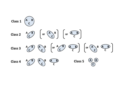
Figure 7: Classification of tripartite entanglement. See text for more details and Ref. tripartite for the definitions of the classes.

Note that the tripartite PPT condition

$$\mathbf{\tilde{V}}_{k}+i\mathbf{\Omega}^{(3)}\geq 0~{}\text{for}~{}k=A,B,C$$ (24)

is not able to distinguish the fully separable states from the three-mode biseparable states (bound entangled). To distinguish between classes $4$ and $5$, we need an additional criterion. Put the CM in the block-form

$$\mathbf{V}=\left(\begin{array}[c]{cc}\mathbf{A}&\mathbf{W}\\ \mathbf{W}^{T}&\mathbf{V}_{BC}\end{array}\right),$$

where $\mathbf{A}$ is the reduced CM of mode $A$, $\mathbf{V}_{BC}$ is reduced CM of modes $B$ and $C$, while $\mathbf{W}$ is a $2\times 4$ block. Using the pseudoinverse, we may construct the test-matrices

$$\mathbf{T} :=\mathbf{A}-\mathbf{W}(\mathbf{V}_{BC}+i\mathbf{\Omega}^{(2)})^{-1}\mathbf{W}^{T},$$ (25)

$$\mathbf{\tilde{T}} :=\mathbf{A}-\mathbf{W}(\mathbf{V}_{BC}+i\boldsymbol{\Lambda}\mathbf{\Omega}^{(2)}\boldsymbol{\Lambda})^{-1}\mathbf{W}^{T},$$ (26)

where $\boldsymbol{\Lambda}$ is the two-mode PT matrix of Eq. (17). Then, a CM satisfying Eq. (24) is fully separable if and only if there exists a single-mode pure-state CM $\mathbb{\sigma}$ such that tripartite

$$\mathbf{T}\geq\mathbb{\sigma},~{}\mathbf{\tilde{T}}\geq\mathbb{\sigma}.$$ (27)

Sec. 2 Theory: Correlated-Thermal Noise

In this section, we consider the Gaussian environment with correlated thermal noise. In such an environmnent, we derive the dynamics of the bosonic modes involved in the basic protocol of entanglement swapping: We study the multipartite separability properties of the state before Bell detection and we compute the CM of the final swapped state analyzing its entanglement. We then study the protocols of quantum teleportation, entanglement distillation, key distillation and practical QKD. In more details, we provide the following elements:

$\bullet~{}$Sec. 2.1: We briefly describe the model of Gaussian environment with correlated-thermal noise, studying its correlations.

$\bullet~{}$Sec. 2.2: Considering the basic swapping protocol, we study the evolution of the bosonic modes, in particular, of the global CM.

$\bullet~{}$Sec. 2.3: We analyze the various forms of entanglement (bipartite, tripartite, and quadripartite) in the output state before the Bell detection.

$\bullet~{}$Sec. 2.4: We apply the Bell detection and compute the CM $\mathbf{V}_{ab|\gamma}(\mu,\kappa,\kappa^{\prime})$ of the swapped state $\rho_{ab|\gamma}$.

$\bullet~{}$Sec. 2.5: We derive the analytical formula for the smallest PTS eigenvalue $\varepsilon(\mu,\kappa,\kappa^{\prime})$ associated with the swapped CM. We can therefore quantify the swapped entanglement. In particular, we discuss the reactivation condition $\kappa\kappa^{\prime}<1$ and its independence from the input entanglement $\mu$. Finally, we derive the asymptotic optimum $\varepsilon_{\text{opt}}$ for large $\mu$.

$\bullet~{}$Sec. 2.6: We discuss our generalized protocol for teleporting coherent states, where Bob’s conditional quantum operation $\mathcal{Q}_{\gamma}$ is tailored to deal with the correlated-thermal environment. We then provide the closed analytical formula for the average teleportation fidelity $F(\mu,\kappa,\kappa^{\prime})$ and we derive its asymptotic optimum $F_{\text{opt}}$ for large $\mu$, connecting $F_{\text{opt}}$ with $\varepsilon_{\text{opt}}$.

$\bullet~{}$Sec. 2.7: We study the distillation protocols. In particular, in Sec. 2.7.1, we study the protocol of entanglement distillation (with one-way classical communication) which is operated on top of entanglement swapping. We compute the analytical formula for the coherent information $I_{\mathcal{C}}(\mu,\kappa,\kappa^{\prime})$, and we derive its optimal expression for large $\mu$, where it becomes a simple function of $\varepsilon_{\text{opt}}$. Then, in Sec. 2.7.2, we discuss the ideal key-distillation protocol based on quantum memories, and we easily show that its rate $K$ is lower-bounded by the coherent information.

$\bullet~{}$Sec. 2.8: We consider the practical QKD protocol where coherent states are sent to a midway relay (which can be untrusted). For this protocol, we derive a closed formula for the secret-key rate $R(\xi,\mu,\kappa,\kappa^{\prime})$ for arbitrary reconciliation efficiency $\xi$ and modulation variance $\mu$. We study the corresponding security threshold $R=0$ for achievable values $\mu\simeq 50$, showing that there is a small difference between ideal reconciliation ($\xi=1$) and realistic reconciliation efficiency ($\xi\simeq 0.97$). Then, we derive the asymptotic optimal rate $R_{\text{opt}}$ considering $\xi=1$ and large $\mu$. The security threshold $R_{\text{opt}}=0$ is shown to be comparable with those achieved at $\mu\simeq 50$. From $R_{\text{opt}}$, we then derive a lower-bound $R_{\text{LB}}$, expressed in terms of $\varepsilon_{\text{opt}}$ and $F_{\text{opt}}$. This bound is sufficiently tight, with its security threshold $R_{\text{LB}}=0$ being very close to $R_{\text{opt}}=0$.

Sec. 2.1 Environment with correlated-thermal noise

Let us first describe the Gaussian environment with correlated-thermal noise. As discussed in the main text, this is modelled by two beam-splitters with transmissivity $\tau$ which mix the input modes $A$ and $B$, with two environmental modes $E_{1}$ and $E_{2}$, prepared in a correlated-noise Gaussian state. This is taken to have zero-mean and CM in the symmetric normal form

$$\mathbf{V}_{E_{1}E_{2}}(\omega,g,g^{\prime})=\left(\begin{array}[c]{cc}\omega\mathbf{I}&\mathbf{G}\\ \mathbf{G}&\omega\mathbf{I}\end{array}\right)~{},$$ (28)

where $\omega\geq 1$ is the variance of thermal noise in each mode, while the block $\mathbf{G}=\mathrm{diag}(g,g^{\prime})$ describes the correlations between modes $E_{1}$ and $E_{2}$. See also Fig. 8, which shows the swapping protocol performed in the presence of this environment.

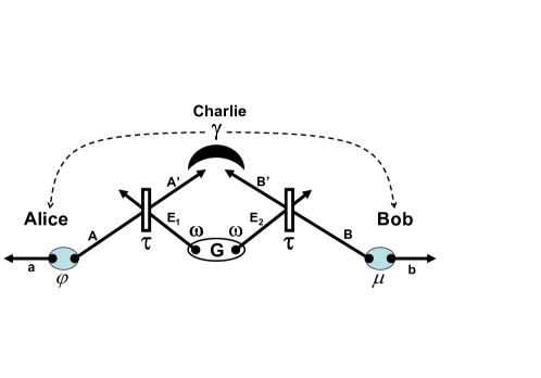
Figure 8: Swapping protocol in the presence of a correlated Gaussian environment with transmissivity $\tau$, thermal noise $\omega$ and noise-correlations $\mathbf{G}$. Bell detector is simplified.

One can derive NJPpirs simple bona-fide conditions in terms of the parameters $\omega\geq 1$, $g$ and $g^{\prime}$. By imposing Eq. (11) to the CM of Eq. (28), one finds the conditions

$$|g|<\omega,~{}~{}|g^{\prime}|<\omega,~{}~{}\omega\left|g+g^{\prime}\right|\leq\omega^{2}+gg^{\prime}-1.$$ (29)

Then, by imposing the separability, i.e., Eq. (18), one finds the additional condition NJPpirs

$$\omega\left|g-g^{\prime}\right|\leq\omega^{2}-gg^{\prime}-1~{}.$$ (30)

For any fixed $\omega\geq 1$, the state of the environment is one-to-one with a point in the correlation plane $(g,g^{\prime})$. Previous conditions in Eq. (29) identify which part of this plane is physically accessible. Then, the addition of Eq. (30) further identifies the region associated with separable environments.

Despite being void of entanglement, separable environments still possess residual quantum correlations. The residual quantum correlations between the two ancillas, $E_{1}$ and $E_{2}$, can be quantified by their quantum discord $D$ RMPdis , which is here symmetric $D(E_{1}|E_{2})=D(E_{2}|E_{1})$. This environmental discord can be expressed in terms of correlation parameters $D=D(g,g^{\prime})$ at any value of thermal noise $\omega$. Similarly, we can compute the (non-discordant) purely-classical correlations $C=C(g,g^{\prime})$ and, therefore, the total separable correlations $I(g,g^{\prime})=C+D$. In Fig. 9, we show the typical maps for $I(g,g^{\prime})$ and $D(g,g^{\prime})$.

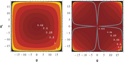
Figure 9: Map of the environmental correlations at fixed thermal noise $\omega=19$. The external black region is excluded, as it corresponds to entangled or unphysical environments. Left panel. We plot the total separable correlations $I(g,g^{\prime})$, corresponding to bits of quantum mutual information. $I(g,g^{\prime})$ increases almost uniformly away from the origin. Note that there is a corresponding plot in the main paper where we consider $\omega=19.38$. Right panel. We plot the Gaussian discord GerryD ; ParisD (in bits) which is proven to be equal to the (unrestricted) quantum discord $D(g,g^{\prime})$ inside the four delimited lobes OptimalDiscord . Discord is non-uniform and rapidly increases along the diagonals of the plane.

Sec. 2.2 Evolution of the bosonic modes

Here we consider the basic swapping protocol of Fig. 8, and we study how Alice’s modes ($a$ and $A$) and Bob’s modes ($b$ and $B$) evolve under the action of Gaussian environment with correlated-thermal noise. Since we are interested in the dynamics of their correlations, we study the evolution of their global CM $\mathbf{V}_{aAbB}\rightarrow\mathbf{V}_{aA^{\prime}bB^{\prime}}$. We start by considering a more general scenario where Alice’s and Bob’s two mode squeezed vacuum (TMSV) states have different variances $\varphi$ and $\mu$. We then specialize our study to the case of symmetric setting $\varphi=\mu$.

As depicted in Fig. 8, we have a total of six input modes: Alice’s modes $a$ and $A$, Bob’s modes $b$ and $B$, and Eve’s modes $E_{1}$ and $E_{2}$. The global input state is the tensor product

$$\rho_{aA}\otimes\rho_{bB}\otimes\rho_{E_{1}E_{2}},$$

where $\rho_{aA}$ and $\rho_{bB}$ are two TMSV states, with CMs $\mathbf{V}(\varphi)$ and $\mathbf{V}(\mu)$, respectively. These are specified by

$$\mathbf{V}(\mu)=\left(\begin{array}[c]{cc}\mu\mathbf{I}&\sqrt{\mu^{2}-1}\mathbf{Z}\\ \sqrt{\mu^{2}-1}\mathbf{Z}&\mu\mathbf{I}\end{array}\right)~{},$$

where $\mu\geq 1$, $\mathbf{I}:=\mathrm{diag}(1,1)$ and $\mathbf{Z}:=\mathrm{diag}(1,-1)$. The environmental state $\rho_{E_{1}E_{2}}$ is Gaussian with zero-mean and CM $\mathbf{V}_{E_{1}E_{2}}(\omega,g,g^{\prime})$ given in Eq. (28). The global input state is a zero-mean Gaussian state with CM

$$\mathbf{V}_{aAbBE_{1}E_{2}}=\mathbf{V}(\varphi)\oplus\mathbf{V}(\mu)\oplus\mathbf{V}_{E_{1}E_{2}}(\omega,g,g^{\prime})~{}.$$

It is helpful to permute the modes so to have the ordering $abAE_{1}E_{2}B$, where the upper-case modes are those transformed by the beam splitters. After reordering, the input CM has the explicit form

$$\mathbf{V}_{abAE_{1}E_{2}B}=\left(\begin{array}[c]{cccccc}\varphi\mathbf{I}&\mathbf{0}&\tilde{\varphi}\mathbf{Z}&\mathbf{0}&\mathbf{0}&\mathbf{0}\\ \mathbf{0}&\mu\mathbf{I}&\mathbf{0}&\mathbf{0}&\mathbf{0}&\tilde{\mu}\mathbf{Z}\\ \tilde{\varphi}\mathbf{Z}&\mathbf{0}&\varphi\mathbf{I}&\mathbf{0}&\mathbf{0}&\mathbf{0}\\ \mathbf{0}&\mathbf{0}&\mathbf{0}&\omega\mathbf{I}&\mathbf{G}&\mathbf{0}\\ \mathbf{0}&\mathbf{0}&\mathbf{0}&\mathbf{G}&\omega\mathbf{I}&\mathbf{0}\\ \mathbf{0}&\tilde{\mu}\mathbf{Z}&\mathbf{0}&\mathbf{0}&\mathbf{0}&\mu\mathbf{I}\end{array}\right)~{},$$

where $\mathbf{0}$ is the $2\times 2$ zero matrix, and we use the notation

$$\tilde{\mu}:=\sqrt{\mu^{2}-1},~{}\tilde{\varphi}:=\sqrt{\varphi^{2}-1}.$$

The global action of the two beam splitters can be represented by the symplectic matrix

$$\mathbf{S=\mathbf{I}}\oplus\mathbf{\mathbf{I}}\oplus\mathbf{S\mathbf{(}}\tau\mathbf{\mathbf{)}\oplus S(}\tau\mathbf{)}^{T}~{},$$

where the identity matrices $\mathbf{\mathbf{I}}\oplus\mathbf{\mathbf{I}}$ act on the remote modes, $a$ and $b$, the beam splitter matrix of Eq. (12) acts on modes $A$ and $E_{1}$, and its transposed $\mathbf{S(}\tau\mathbf{)}^{T}$ acts on modes $E_{2}$ and $B$. In the following calculations we exclude the trivial and singular case of $\tau=0$.

The output state of modes $abA^{\prime}E_{1}^{\prime}E_{2}^{\prime}B^{\prime}$ after the action of the interferometer is a Gaussian state with zero mean and CM equal to

$$\mathbf{V}_{abA^{\prime}E_{1}^{\prime}E_{2}^{\prime}B^{\prime}}=\mathbf{S~{}V}_{abAE_{1}E_{2}B}~{}\mathbf{S}^{T}~{}.$$

Since we are interested in the CM of Alice and Bob, we trace out the two environmental modes $E_{1}^{\prime}$ and $E_{2}^{\prime}$. As a result, we get the following CM for modes $abA^{\prime}B^{\prime}$

$$\mathbf{V}_{abA^{\prime}B^{\prime}}(\varphi,\mu,\tau,\omega,g,g^{\prime})$$

$$=\left(\begin{array}[c]{cccc}\varphi\mathbf{I}&\mathbf{0}&\tilde{\varphi}\sqrt{\tau}\mathbf{Z}&\mathbf{0}\\ \mathbf{0}&\mu\mathbf{I}&\mathbf{0}&\tilde{\mu}\sqrt{\tau}\mathbf{Z}\\ \tilde{\varphi}\sqrt{\tau}\mathbf{Z}&\mathbf{0}&y\mathbf{I}&(1-\tau)\mathbf{G}\\ \mathbf{0}&\tilde{\mu}\sqrt{\tau}\mathbf{Z}&(1-\tau)\mathbf{G}&x\mathbf{I}\end{array}\right),$$ (35)

where

$$y:=\tau\varphi+(1-\tau)\omega,~{}x:=\tau\mu+(1-\tau)\omega~{}.$$

Sec. 2.3 Output entanglement before Bell detection

It is important to study the evolution of quantum entanglement under the Gaussian environment with correlated-thermal noise. For this analysis we consider the symmetric case $\varphi=\mu$, so that

$$\mathbf{V}_{abA^{\prime}B^{\prime}}=\left(\begin{array}[c]{cccc}\mu\mathbf{I}&\mathbf{0}&\tilde{\mu}\sqrt{\tau}\mathbf{Z}&\mathbf{0}\\ \mathbf{0}&\mu\mathbf{I}&\mathbf{0}&\tilde{\mu}\sqrt{\tau}\mathbf{Z}\\ \tilde{\mu}\sqrt{\tau}\mathbf{Z}&\mathbf{0}&x\mathbf{I}&(1-\tau)\mathbf{G}\\ \mathbf{0}&\tilde{\mu}\sqrt{\tau}\mathbf{Z}&(1-\tau)\mathbf{G}&x\mathbf{I}\end{array}\right).$$ (36)

From this CM, we can derive all the reduced CMs and analyze all the various forms of output entanglement: Bipartite, tripartite and quadripartite. For simplicity, we also consider the limit of large entanglement at the input, i.e., $\mu\gg 1$. This limit not only simplifies the analytical formulas but also optimizes the scheme: If entanglement is broken in this limit, then it must be broken for any finite value of $\mu$. Indeed, for $\mu\gg 1$, a TMSV state becomes an ideal EPR source, i.e., a CV maximally-entangled (asymptotic) state, and the entanglement-breaking conditions for this state can be extended to all the others. In the derivations of this section we also implicitly assume that $\tau<1$.

Sec. 2.3.1 Bipartite entanglement

Let us start from bipartite entanglement. By symmetry, it is sufficient to study the pairings $aA^{\prime}$, $aB^{\prime}$, $ab$ and $A^{\prime}B^{\prime}$. The pairing $ab$ is trivial to consider since the two remote modes are manifestly separable before Bell detection, as one can also check from their reduced CM $\mathbf{V}_{ab}=\mu\mathbf{I}\oplus\mu\mathbf{I}$. It is also trivial to check the pairing $aB^{\prime}$, for which we have $\mathbf{V}_{aB^{\prime}}=\mu\mathbf{I}\oplus x\mathbf{I}$. Regarding the pairing $A^{\prime}B^{\prime}$, we can check that $\rho_{A^{\prime}B^{\prime}}$ is separable for large $\mu$. In fact, from the reduced CM $\mathbf{V}_{A^{\prime}B^{\prime}}$ we compute the log-negativity

$$\mathcal{N}_{A^{\prime}B^{\prime}}=\max\left\{0,-\log_{2}\left[\tau\mu+\frac{1-\tau}{2}(2\omega-|g-g^{\prime}|)\right]\right\},$$

which is always zero for large $\mu$ and $\tau>0$. In the singular case $\tau=0$, we have $\rho_{A^{\prime}B^{\prime}}=\rho_{E_{1}E_{2}}$ so that separability directly comes from the (separable) environment.

The most interesting pairing is $aA^{\prime}$. From the reduced CM $\mathbf{V}_{aA^{\prime}}$, we can compute the log-negativity $\mathcal{N}_{aA^{\prime}}$. For large $\mu$, we find

$$\mathcal{N}_{aA^{\prime}}=\max\left\{0,\log_{2}\left[\frac{1+\tau}{(1-\tau)\omega}\right]\right\},$$

so that bipartite entanglement is lost ($\mathcal{N}_{aA^{\prime}}=0$) for

$$\omega\geq\omega_{\text{EB}}(\tau):=\frac{1+\tau}{1-\tau},$$

which is the known entanglement-breaking threshold of the lossy channel.

Thus, the threshold condition $\omega=\omega_{\text{EB}}(\tau)$ guarantees that bipartite entanglement is broken between any pairing of two modes, no matter how strong are the correlations in the separable environment. See also Fig. 10.

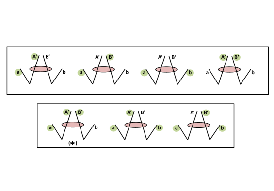
Figure 10: Upper panel. Study of the bipartite entanglement. At the threshold condition $\omega=\omega_{\text{EB}}$, there is no entanglement surviving between any two modes in the scheme. By symmetry it is sufficient to consider the pairings $aA^{\prime}$, $aB^{\prime}$, $ab$, and $A^{\prime}B^{\prime}$ (from left to right). Lower Panel. Study of the tripartite entanglement. At the threshold condition $\omega=\omega_{\text{EB}}$, there is no tripartite entanglement in the triplets $aA^{\prime}b$ and $aB^{\prime}b$ (fully separable, i.e., class 5). Different is the case for the triplet $aA^{\prime}B^{\prime}$, denoted by (*) in the panel. Here the tripartite entanglement is broken if we assume the strict inequality $\omega>\omega_{\text{EB}}$. At exactly $\omega=\omega_{\text{EB}}$ the tripartite state of $aA^{\prime}B^{\prime}$ is guaranteed to be fully separable only if there are no correlations in the environment ($g=g^{\prime}=0$), otherwise it is a one-mode biseparable state (class 2 entanglement).

Sec. 2.3.2 Tripartite entanglement

Thanks to the symmetry of the configuration, it is sufficient to study the triplets of modes $aA^{\prime}B^{\prime}$, $aA^{\prime}b$ and $aB^{\prime}b$, shown in Fig. 10. Two of these cases are very easy to study. In fact, from the CM of Eq. (36) we see that

$$\mathbf{V}_{aA^{\prime}b} =\mathbf{V}_{aA^{\prime}}\oplus\mathbf{V}_{b},$$

$$\mathbf{V}_{aB^{\prime}b} =\mathbf{V}_{a}\oplus\mathbf{V}_{B^{\prime}b},$$

which means that $\rho_{aA^{\prime}b}=\rho_{aA^{\prime}}\otimes\rho_{b}$ and $\rho_{aB^{\prime}b}=\rho_{a}\otimes\rho_{B^{\prime}b}$. Because of this tensor product structure, the absence of bipartite entanglement (in $aA^{\prime}$ and $B^{\prime}b$) implies the absence of tripartite entanglement. Thus, the previous threshold condition $\omega=\omega_{\text{EB}}(\tau)$ also breaks tripartite entanglement in $aA^{\prime}b$ and $aB^{\prime}b$.

More involved is the situation for the triplet $aA^{\prime}B^{\prime}$. First of all we study the positivity of the three matrices

$$\mathbf{W}_{k}:=\boldsymbol{\Lambda}_{k}\mathbf{V}_{aA^{\prime}B^{\prime}}\boldsymbol{\Lambda}_{k}+i\mathbf{\Omega}^{(3)},$$

with $k=a$, $A^{\prime}$ and $B^{\prime}$ (here $\boldsymbol{\Lambda}_{k}$ is the usual PT matrix with block $\mathbf{Z}$ being applied to mode $k$). Since the matrices $\mathbf{W}_{k}$ are Hermitian, the positive-semidefiniteness $\mathbf{W}_{k}\geq 0$ is equivalent to check the non-negativity of their eigenvalues or, equivalently, their principal minors (more easily, the positive-definiteness $\mathbf{W}_{k}>0$ is equivalent to check the strict positivity of the eigenvalues or the leading principal minors). If all these matrices are $\mathbf{W}_{k}\geq 0$, i.e., the tripartite state is PPT, then we apply the criterion of Eq. (27) to distinguish class 4 and 5. In particular, note that $\mathbf{T}-\mathbb{\sigma}$ and $\mathbf{\tilde{T}}-\mathbb{\sigma}$ are Hermitian matrices.

Markovian case

In the absence of correlations ($g=g^{\prime}=0$), one can check that the threshold condition $\omega=\omega_{\text{EB}}(\tau)$ is sufficient to destroy tripartite entanglement in $aA^{\prime}B^{\prime}$. In fact, in these conditions, the eigenvalues of the three matrices $\mathbf{W}_{k}$ are all non-negative, which means that $\rho_{aA^{\prime}B^{\prime}}$ is a PPT state. Then, we also find that the test matrices of Eqs. (25) and (26) satisfy $\mathbf{T}\geq\mathbf{I}$ and $\mathbf{\tilde{T}}\geq\mathbf{I}$ (where the identity $\mathbf{I}$ is the CM of the vacuum state). More precisely, the two Hermitian matrices $\mathbf{T}-\mathbf{I}$ and $\mathbf{\tilde{T}}-\mathbf{I}$ have the same non-negative spectrum of eigenvalues $\left\{0,2(\mu-1)[2+\tau(\mu+1)]^{-1}\right\}$ for any $\mu\geq 1$. As a result, we find that $\rho_{aA^{\prime}B^{\prime}}$ is a fully separable state (class 5).

Non-Markovian case

In the presence of correlations, i.e., for $(g,g^{\prime})\neq(0,0)$, the threshold condition $\omega=\omega_{\text{EB}}(\tau)$ does not break tripartite entanglement. In fact, in the limit of large $\mu$, we find that both $\det\mathbf{W}_{1}$ and $\det\mathbf{W}_{2}$ are negative, so that $\mathbf{W}_{1},\mathbf{W}_{2}\ngeq 0$. Then, by studying its leading principal minors, we find that $\mathbf{W}_{3}>0$. This means that the state $\rho_{aA^{\prime}B^{\prime}}$ remains one-mode biseparable (entanglement class 2).

However, the strict violation $\omega>\omega_{\text{EB}}(\tau)$ is sufficient to break tripartite entanglement. In this case, for large $\mu$, we find that the leading principal minors of $\mathbf{W}_{1}$, $\mathbf{W}_{2}$, and $\mathbf{W}_{3}$ are all strictly positive. Then, we also find that $\mathbf{T}-\mathbf{I}$ and $\mathbf{\tilde{T}}-\mathbf{I}$ have the same spectrum with strictly-positive eigenvalues. As a result, the state $\rho_{aA^{\prime}B^{\prime}}$ becomes fully separable (class 5).

Sec. 2.3.3 Quadripartite entanglement

From the previous discussion, we conclude that the condition $\omega>\omega_{\text{EB}}(\tau)$ is able to break both bipartite and tripartite entanglement, considering all possible combinations of bipartite and tripartite states in our scheme. This is true both in the Markovian and non-Markovian case (with separable correlations in the environment). But what about the separability properties of the global quadri-partite state $\rho_{abA^{\prime}B^{\prime}}$?

By exploiting the multipartite PPT criterion of Eq. (23), we can study the separability of the quadri-partite state with respect to the $1\times 3$ groupings of the modes $abA^{\prime}B^{\prime}$. Because of the symmetry between Alice and Bob, it is sufficient to consider the two groupings

$$\{a\}\{bA^{\prime}B^{\prime}\},~{}\{A^{\prime}\}\{abB^{\prime}\},$$ (37)

which can be labelled by $k=a$ and $k=A^{\prime}$, respectively (with corresponding PT matrices $\boldsymbol{\Lambda}_{a}$ and $\boldsymbol{\Lambda}_{A^{\prime}}$). Thus, we compute the two matrices

$$\mathbf{M}_{k}:=\boldsymbol{\Lambda}_{k}\mathbf{V}_{abA^{\prime}B^{\prime}}\boldsymbol{\Lambda}_{k}+i\mathbf{\Omega}^{(4)}.$$

Assuming $\omega>\omega_{\text{EB}}(\tau)$ and large $\mu$, we study the positivity properties of the matrices $\mathbf{M}_{k}$, finding that they can be expressed in terms of analytical functions. Set $\omega=r~{}\omega_{\text{EB}}(\tau)$ with $r>1$. Then we define

$$\Sigma^{\prime}:=\min\{f,f^{\prime}\},~{}\Sigma^{\prime\prime}:=\min\{f,f^{\prime\prime}\},$$

where

$$f :=(1+\tau)^{2}(r^{2}-1)-g^{2}(1-\tau)^{2},$$

$$f^{\prime} :=(1-\tau)^{2}[1+\tau-gg^{\prime}(1-\tau)]^{2}+\zeta,$$

$$f^{\prime\prime} :=(1-\tau)^{2}[1+\tau+gg^{\prime}(1-\tau)]^{2}+\zeta,$$

and

$$\zeta:=(1+\tau)^{4}r^{4}-(1+\tau)^{2}[2+g^{2}(1-\tau)^{2}+g^{\prime 2}(1-\tau)^{2}+2\tau^{2}]r^{2}.$$

Using these functions, we can write the implications

$$\Sigma^{\prime} >0\Longleftrightarrow\mathbf{M}_{a}>0\Longrightarrow\{a\}\{bA^{\prime}B^{\prime}\}\text{ separable,}$$

$$\Sigma^{\prime} <0\Longrightarrow\mathbf{M}_{a}\ngeq 0\Longleftrightarrow\{a\}\{bA^{\prime}B^{\prime}\}\text{ entangled.}$$

Despite the fact that the border condition $\Sigma^{\prime}=0$ is inconclusive, we find that it only occurs in a set of zero measure within the correlation plane $(g,g^{\prime})$. As a result, $\Sigma^{\prime}=0$ clearly distinguishes the region where the state is separable from that where it is entangled, with respect to the grouping $\{a\}\{bA^{\prime}B^{\prime}\}$.

Similarly, we can write the following implications for the other grouping of modes

$$\Sigma^{\prime\prime} >0\Longleftrightarrow\mathbf{M}_{A^{\prime}}>0\Longrightarrow\{A^{\prime}\}\{abB^{\prime}\}\text{ separable,}$$

$$\Sigma^{\prime\prime} <0\Longrightarrow\mathbf{M}_{A^{\prime}}\ngeq 0\Longleftrightarrow\{A^{\prime}\}\{abB^{\prime}\}\text{ entangled,}$$

with the border condition $\Sigma^{\prime\prime}=0$ distinguishing between regions of separability and entanglement.

Altogether, we can identify four regions for the quadripartite state $\rho_{abA^{\prime}B^{\prime}}$:

(I)

$\Sigma^{\prime},\Sigma^{\prime\prime}>0$: Separable in all the $1\times 3$ groupings,

(II)

$\Sigma^{\prime}>0$ and $\Sigma^{\prime\prime}<0$: Entangled in $\{A^{\prime}\}\{abB^{\prime}\}$,

(III)

$\Sigma^{\prime}<0$ and $\Sigma^{\prime\prime}>0$: Entangled in $\{a\}\{bA^{\prime}B^{\prime}\}$,

(IV)

$\Sigma^{\prime},\Sigma^{\prime\prime}<0$: Entangled in all the $1\times 3$ groupings.

These regions are numerically shown in Fig. 11. As we can see from the figure, $1\times 3$ quadri-partite entanglement is reactivated after a certain amount of separable correlations is injected by the environment. This critical amount increases in the thermal noise $\omega>\omega_{\text{EB}}(\tau)$. For instance, this is evident by comparing panel (c), where $r=1.02$, with panel (a), where $r=1.1$. By increasing the thermal noise, region (I) widens while region (IV) shrinks. Also note that, by increasing the transmissivity $\tau$ (while keeping $r$ fixed), the two regions (II) and (III) tend to coincide. For instance, compare panel (a) with panel (b), and panel (c) with panel (d). We have checked that this behavior is generic and also occurs at finite $\mu$, where we have studied the positivity properties of the matrices $\mathbf{M}_{k}$ by (numerically) computing their spectra.

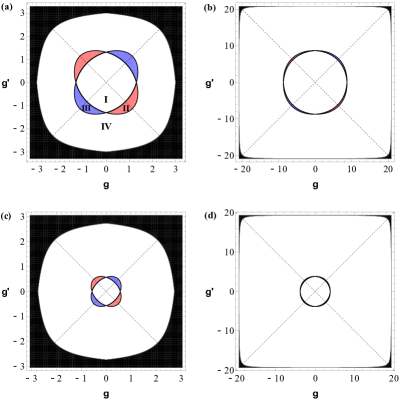
Figure 11: Study of the quadripartite entanglement of the state $\rho_{abA^{\prime}B^{\prime}}$ on the correlation plane. In each panel, we plot the border conditions $\Sigma^{\prime}=0$ and $\Sigma^{\prime\prime}=0$, which result in two different intersecting curves. The most inner region (I) corresponds to $1\times 3$ separability. The red region (II) corresponds to entanglement with respect to the grouping $\{A^{\prime}\}\{abB^{\prime}\}$. The blue region (III) corresponds to entanglement with respect to the grouping $\{a\}\{bA^{\prime}B^{\prime}\}$. Finally, the outer region (IV) corresponds to entanglement in all the groupings. Here we consider: $r=1.1$ and $\tau=0.5$ in panel (a), $r=1.1$ and $\tau=0.9$ in panel (b), $r=1.02$ and $\tau=0.5$ in panel (c), and $r=1.02$ and $\tau=0.9$ in panel (d).

In conclusion, we find that, despite the condition $\omega>\omega_{\text{EB}}(\tau)$ is able to break bipartite and tripartite entanglement, there could be a survival of quadri-partite $1\times 3$ entanglement, whose existence depends on the amount of separable correlations injected by the environment. In particular, this entanglement can be reactivated with respect to the grouping $\{a\}\{bA^{\prime}B^{\prime}\}$. In this case, a quantum measurement on modes $A^{\prime}$ and $B^{\prime}$ can localize this multi-partite resource in the remaining modes $a$ and $b$ (thus generating bipartite entanglement). A simple (but presumably sub-optimal) way to localize this quadri-partite entanglement is the use of the Bell detection. If the procedure is successful, then the protocol of entanglement swapping can be reactivated from entanglement-breaking (see Sec. 2.4 and Sec. 2.5).

Note that we have not analyzed quadripartite entanglement of the $2\times 2$ type, associated with the groupings $\{ab\}\{A^{\prime}B^{\prime}\}$, $\{aA^{\prime}\}\{bB^{\prime}\}$, or $\{aB^{\prime}\}\{bA^{\prime}\}$. In the Markovian case ($g=g^{\prime}=0$), this is certainly absent for $\omega>\omega_{\text{EB}}(\tau)$. In the non-Markovian case this type of entanglement could potentially be reactivated by the separable correlations of the environment. However, this analysis not only is involved but also secondary, since the reactivation of $1\times 3$ quadripartite entanglement (always distillable quadripartite ) is already sufficient to induce the localization into a bipartite form.

Sec. 2.4 Covariance Matrix of the Swapped State

To study the protocol of entanglement swapping in general non-Markovian conditions, the first step is the computation of the CM $\mathbf{V}_{ab|\gamma}$ of the swapped state $\rho_{ab|\gamma}$, after Bell detection. Here we start by considering an asymmetric scenario, where Alice and Bob may have different EPR resources (TMSV states). We then specify the formula to the case of identical resources.

Starting from the CM of Eq. (35), we compute the CM $\mathbf{V}_{ab|\gamma}$ of the conditional remote state $\rho_{ab|\gamma}$ by applying the transformation rules for CMs under Bell-like measurements specified in Ref. BellFORMULA . As a first step, we put $\mathbf{V}_{abA^{\prime}B^{\prime}}$ in the blockform

$$\mathbf{V}_{abA^{\prime}B^{\prime}}=\left(\begin{array}[c]{ccc}\mathbf{V}_{ab}&\mathbf{C}_{1}&\mathbf{C}_{2}\\ \mathbf{C}_{1}^{T}&\mathbf{B}_{1}&\mathbf{D}\\ \mathbf{C}_{2}^{T}&\mathbf{D}^{T}&\mathbf{B}_{2}\end{array}\right)~{},$$

where

$$\mathbf{B}_{1}=y\mathbf{I,~{}B}_{2}=x\mathbf{I,~{}D}=(1-\tau)\mathbf{G,}$$

and

$$\mathbf{C}_{1}=\left(\begin{array}[c]{c}\tilde{\varphi}\sqrt{\tau}\mathbf{Z}\\ \mathbf{0}\end{array}\right),~{}\mathbf{C}_{2}=\left(\begin{array}[c]{c}\mathbf{0}\\ \tilde{\mu}\sqrt{\tau}\mathbf{Z}\end{array}\right).$$

Then the conditional CM is given by the formula BellFORMULA

$$\mathbf{V}_{ab|\gamma}=\mathbf{V}_{ab}-\frac{1}{2\det\boldsymbol{\Theta}}\sum_{i,j=1}^{2}\mathbf{C}_{i}(\mathbf{X}_{i}^{T}\boldsymbol{\Theta}\mathbf{X}_{j})\mathbf{C}_{j}^{T}~{},$$

where

$$\mathbf{X}_{1}:=\left(\begin{array}[c]{cc}0&1\\ 1&0\end{array}\right),~{}\mathbf{X}_{2}:=\left(\begin{array}[c]{cc}0&1\\ -1&0\end{array}\right)~{},$$

and

$$\boldsymbol{\Theta}:=\frac{1}{2}\left(\mathbf{ZB}_{1}\mathbf{Z}+\mathbf{B}_{2}-\mathbf{ZD}-\mathbf{D}^{T}\mathbf{Z}\right)=\left(\begin{array}[c]{cc}\theta&0\\ 0&\theta^{\prime}\end{array}\right)$$

with diagonal terms

$$\left\{\begin{array}[c]{c}\theta:=\frac{\tau}{2}(\varphi+\mu)+(1-\tau)(\omega-g),\\ \\ \theta^{\prime}:=\frac{\tau}{2}(\varphi+\mu)+(1-\tau)(\omega+g^{\prime}).\end{array}\right.$$

After simple algebra, we derive the following expression for the conditional CM

$$\mathbf{V}_{ab|\gamma}=\left(\begin{array}[c]{cc}\varphi\mathbf{I}&\mathbf{0}\\ \mathbf{0}&\mu\mathbf{I}\end{array}\right)-\frac{\tau}{2}\left(\begin{array}[c]{cccc}\frac{\tilde{\varphi}^{2}}{\theta}&0&-\frac{\tilde{\varphi}\tilde{\mu}}{\theta}&0\\ 0&\frac{\tilde{\varphi}^{2}}{\theta^{\prime}}&0&\frac{\tilde{\varphi}\tilde{\mu}}{\theta^{\prime}}\\ -\frac{\tilde{\varphi}\tilde{\mu}}{\theta}&0&\frac{\tilde{\mu}^{2}}{\theta}&0\\ 0&\frac{\tilde{\varphi}\tilde{\mu}}{\theta^{\prime}}&0&\frac{\tilde{\mu}^{2}}{\theta^{\prime}}\end{array}\right).$$ (38)

In the symmetric case of identical EPR sources (TMSV states), i.e., for $\varphi=\mu$, the conditional CM $\mathbf{V}_{ab|\gamma}$ of Eq. (38) takes the following simple form

$$\mathbf{V}_{ab|\gamma}=\left(\begin{array}[c]{cc}\mu\mathbf{I}&\mathbf{0}\\ \mathbf{0}&\mu\mathbf{I}\end{array}\right)-\frac{\mu^{2}-1}{2}\boldsymbol{\Psi}~{},$$ (39)

where

$$\boldsymbol{\Psi}=\left(\begin{array}[c]{cccc}\frac{1}{\mu+\kappa}&0&\frac{-1}{\mu+\kappa}&0\\ 0&\frac{1}{\mu+\kappa^{\prime}}&0&\frac{1}{\mu+\kappa^{\prime}}\\ \frac{-1}{\mu+\kappa}&0&\frac{1}{\mu+\kappa}&0\\ 0&\frac{1}{\mu+\kappa^{\prime}}&0&\frac{1}{\mu+\kappa^{\prime}}\end{array}\right),$$ (40)

with

$$\left\{\begin{array}[c]{c}\kappa:=(\tau^{-1}-1)(\omega-g)\geq 0~{},\\ \\ \kappa^{\prime}:=(\tau^{-1}-1)(\omega+g^{\prime})\geq 0~{}.\end{array}\right.$$ (41)

The CM of Eq. (39) can be put in the blockform

$$\mathbf{V}_{ab|\gamma}=\left(\begin{array}[c]{cc}\mathbf{A}&\mathbf{C}\\ \mathbf{C}^{T}&\mathbf{B}\end{array}\right),$$ (42)

where

$$\mathbf{A} =\mathbf{B}=\left(\begin{array}[c]{cc}\mu-\frac{\mu^{2}-1}{2(\mu+\kappa)}&0\\ 0&\mu-\frac{\mu^{2}-1}{2(\mu+\kappa^{\prime})}\end{array}\right),$$ (45)

$$\mathbf{C} =\left(\begin{array}[c]{cc}\frac{\mu^{2}-1}{2(\mu+\kappa)}&0\\ 0&-\frac{\mu^{2}-1}{2(\mu+\kappa^{\prime})}\end{array}\right),$$ (48)

which is the expression in Eqs. (1)-(3) of the main text.

It is clear that the CM $\mathbf{V}_{ab|\gamma}$ of the swapped state $\rho_{ab|\gamma}$ does not depend on the specific outcome $\gamma$ of the Bell detection, which only affects the first moments of the state (the CM is only conditioned by the fact that the Bell detection has been performed and the outcome communicated). Also note that the conditional CM $\mathbf{V}_{ab|\gamma}$ is symmetric under $a-b$ permutation.

For the next calculations it is helpful to derive the symplectic spectrum of the CM $\mathbf{V}_{ab|\gamma}$. This is given by RMP

$$\nu_{\pm}=\sqrt{\frac{\Delta\pm\sqrt{\Delta^{2}-4\det\mathbf{V}_{ab|\gamma}}}{2}},$$

where the symplectic invariant $\Delta:=\det\mathbf{A}+\det\mathbf{B}+2\det\mathbf{C}$ is computed from the blocks in Eqs. (45) and (48). After simple algebra we find

$$\{\nu_{-},\nu_{+}\}=\left\{\sqrt{\frac{\mu(1+\mu\kappa)}{\mu+\kappa}},~{}\sqrt{\frac{\mu(1+\mu\kappa^{\prime})}{\mu+\kappa^{\prime}}}\right\}.$$ (49)

It is also useful to derive the symplectic eigenvalue of the reduced CM $\mathbf{V}_{b|\gamma}=\mathbf{B}$, which describes Bob’s reduced state $\rho_{b|\gamma}$. This is just given by

$$\nu_{b}=\sqrt{\det\mathbf{B}}=\frac{1}{2}\sqrt{\frac{(1+2\mu\kappa+\mu^{2})(1+2\mu\kappa^{\prime}+\mu^{2})}{(\mu+\kappa)(\mu+\kappa^{\prime})}}.$$ (50)

Sec. 2.5 Quantification of the Swapped Entanglement

Let us consider the symmetric scenario $\varphi=\mu$. In order to quantify the amount of entanglement which is present in the swapped state $\rho_{ab|\gamma}$, we compute the smallest PTS eigenvalue of the CM $\mathbf{V}_{ab|\gamma}$. This is given by RMP

$$\varepsilon=\sqrt{\frac{\Sigma-\sqrt{\Sigma^{2}-4\det\mathbf{V}_{ab|\gamma}}}{2}},$$

where $\Sigma:=\det\mathbf{A}+\det\mathbf{B}-2\det\mathbf{C}$ is computed from the blocks in Eqs. (45) and (48). After simple algebra we find

$$\varepsilon=\sqrt{\frac{(1+\mu\kappa)(1+\mu\kappa^{\prime})}{(\mu+\kappa)(\mu+\kappa^{\prime})}}$$ (51)

with $\kappa$ and $\kappa^{\prime}$ specified by Eq. (41). Also note that $\varepsilon=\nu_{-}\nu_{+}\mu^{-1}$, where the $\nu$’s are the eigenvalues in Eq. (49).

We can easily check that the presence of entanglement in the swapped state ($\varepsilon<1$) is equivalent to the condition $\kappa\kappa^{\prime}<1$ for any $\mu>1$. In other words, as long as input entanglement is present (i.e., $\mu>1$), the success of entanglement swapping corresponds to $\kappa\kappa^{\prime}<1$, no matter how much entangled the input was (i.e., independently from the actual value of $\mu>1$). It is however true that the amount of the swapped entanglement, e.g., as quantified by the log-negativity logNEG ; logNEG2 $\mathcal{N}=\max\{0,-\log_{2}\varepsilon\}$, depends on the value of $\mu$, as we can see from Eq. (51). One can check that $\frac{d\mathcal{N}}{d\mu}>0$ for $\kappa\kappa^{\prime}<1$, so that the amount of entanglement increases in $\mu$. The maximal swapped entanglement is achieved in the limit of infinite input entanglement $\mu\gg 1$, so that the previous eigenvalue becomes

$$\varepsilon\rightarrow\varepsilon_{\text{opt}}:=\sqrt{\kappa\kappa^{\prime}}=(\tau^{-1}-1)\sqrt{(\omega-g)(\omega+g^{\prime})}.$$ (52)

Note that, for antisymmetric correlations $g+g^{\prime}=0$ (i.e., $\kappa=\kappa^{\prime}$), we have

$$\varepsilon=\frac{1+\mu\kappa}{\mu+\kappa}~{},$$

which is less than $1$ when $\kappa<1$. In the specific case of a Markovian environment ($g=g^{\prime}=0$), we have $\kappa=\kappa^{\prime}=(\tau^{-1}-1)\omega$ and the condition $\kappa<1$ corresponds to $\omega<\tau(1-\tau)^{-1}$. Such condition is clearly not satisfied assuming entanglement-breaking

$$\omega>\omega_{\text{EB}}(\tau)=(1+\tau)(1-\tau)^{-1}~{}.$$

As we discuss in the main text, the situation is different when the Gaussian environment is non-Markovian with separable correlations. In this case, we can swap entanglement ($\varepsilon<1$) even if $\omega>\omega_{\text{EB}}(\tau)$. Imposing $\kappa\kappa^{\prime}=1$, we can write a threshold condition for the correlation parameters $g$ and $g^{\prime}$ at any transmissivity $\tau$, which can be expressed as

$$g=\frac{1+2\tau+g^{\prime}(1-\tau^{2})}{1-\tau^{2}+g^{\prime}(1-\tau)^{2}}~{}.$$

For any $g$ exceeding such a threshold, entanglement swapping is reactivated. In general, the reactivation condition $\kappa\kappa^{\prime}<1$ corresponds to a region of the correlation plane $(g,g^{\prime})$ as shown in Fig. 12.

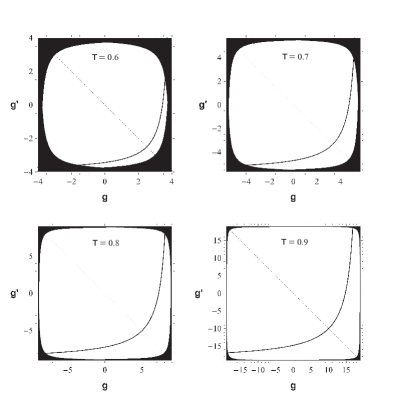
Figure 12: In each panel, the white regions correspond to bona-fide separable Gaussian environments. We plot the threshold condition $\kappa\kappa^{\prime}=1$ (solid curve). For any point $(g,g^{\prime})$ below the threshold, we have $\kappa\kappa^{\prime}<1$ which means that entanglement swapping is reactivated. Here we consider $\tau=0.6$, $0.7$, $0.8$, and $0.9$ from top-left to bottom-right, and corresponding entanglement-breaking values of the thermal noise $\omega=r~{}\omega_{\text{EB}}(\tau)$, with $r=1+10^{-4}$. The value of $\mu$ is arbitrary as long as $\mu>1$ (i.e., input entanglement is present).

Sec. 2.6 Quantum Teleportation of Coherent States

Here we analytically compute the average fidelity for the teleportation protocol in the presence of the non-Markovian Gaussian environment with correlated thermal noise. Consider a symmetric protocol of teleportation, where one party, Alice, aims to teleport an unknown coherent state $\left|\nu\right\rangle$ to the another party, Bob, using a middle station as teleporter, Charlie. As depicted in Fig. 13(i), Alice sends her coherent state $\left|\nu\right\rangle$ to Charlie, who also receives part $B$ of a TMSV state $\rho_{Bb}$ from Bob, with variance $\mu$. These two transmissions are affected by the correlated-noise Gaussian environment with links’ transmissivity $\tau$, thermal noise variance $\omega$, and correlations $\mathbf{G}=\mathrm{diag}(g,g^{\prime})$. Then, Charlie performs a Bell detection and communicates the outcome $\gamma$ to Bob, therefore projecting his mode $b$ onto a conditional state $\rho_{b|\gamma}(\nu)$.

On this state, Bob applies a conditional quantum operation $\mathcal{Q}_{\gamma}$ which provides the teleported output state $\rho_{\text{out}}(\nu)\approx\left|\nu\right\rangle\left\langle\nu\right|$. Bob’s conditional operation $\mathcal{Q}_{\gamma}$ can be broken down in two subsequent operations, first a conditional displacement $D_{b|\gamma}$ (erasing the shift coming from the measurement), and then a suitably-optimized quantum operation $\mathcal{Q}$ which aims to correct the perturbation of the noisy environment (as we will see afterwards, this operation $\mathcal{Q}$ is in turn broken down into a squeezing unitary followed by a quantum amplifier RMP ).

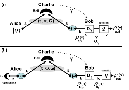
Figure 13: (i) Teleportation and (ii) Measurement-based scheme for teleportation. See text for more explanations.

As shown in Fig. 13(ii), this protocol can equivalently be described as a measurement-based teleportation. Here Alice has another TMSV state $\rho_{aA}$ (with variance $\varphi$) whose mode $a$ is subject to a heterodyne detection with complex outcome $\alpha=(q+ip)/2$, equivalently denoted by the real vector $\mathbf{a}=(q,p)^{T}$. This prepares a coherent state on mode $A$, with randomly-modulated amplitude $\nu(\alpha)=\tilde{\varphi}(\varphi+1)^{-1}\alpha^{\ast}$, where $\alpha$ follows a complex Gaussian distribution $p(\alpha)$ with zero mean and variance $\varphi-1$. Equivalently, the coherent state has mean-value $\mathbf{\bar{x}}_{A|\alpha}=\tilde{\varphi}(\varphi+1)^{-1}\mathbf{Za}$, which is modulated by a bivariate Gaussian distribution with zero mean and variance $\varphi-1$. This can be proven by using the formulas for the heterodyne detection which can be found in Ref. HET (see also Supplementary Material of Ref. OptimalDiscord for all details on the remote preparation of one-mode Gaussian states by using local Gaussian measurements on two-mode Gaussian states). In the limit $\varphi\gg 1$, the coherent state has amplitude $\alpha^{\ast}$ and mean-value $\mathbf{Za}$, uniformly picked from the entire phase-space.

From the point of view of Bob, the measurements of Alice and Charlie permute, so that we can equivalently assume that the Bell detection occurs before the heterodyne detection. As a result, Bob’s conditional state $\rho_{b|\gamma}(\alpha)$ can be derived by applying the heterodyne POVM $\{\Pi_{a}(\alpha)\}$ to the $a$ mode of the swapped state $\rho_{ab|\gamma}$, i.e., we have

$$\rho_{b|\gamma}(\alpha)=p(\alpha|\gamma)^{-1}\mathrm{Tr}_{a}[\Pi_{a}(\alpha)\rho_{ab|\gamma}].$$

The teleported state is therefore given by

$$\rho_{\text{out}}(\alpha)=\mathcal{Q}[D_{b|\gamma}~{}\rho_{b|\gamma}(\alpha)~{}D_{b|\gamma}^{\dagger}],$$

with outcome-dependent fidelity

$$F(\alpha):=\left\langle\nu(\alpha)\right|\rho_{\text{out}}(\alpha)\left|\nu(\alpha)\right\rangle.$$

The average teleportation fidelity is finally given by

$$F=\int d^{2}\alpha~{}p(\alpha)F(\alpha).$$ (53)

Note that we may alternatively write

$$\rho_{\text{out}}(\alpha)=\mathcal{Q}[\rho_{b_{0}}(\alpha)]$$

where

$$\rho_{b_{0}}(\alpha) =p(\alpha|\gamma)^{-1}\mathrm{Tr}_{a}[\Pi_{a}(\alpha)\rho_{ab|\gamma}(0)]~{},$$

$$\rho_{ab|\gamma}(0) :=D_{b|\gamma}\rho_{ab|\gamma}D_{b|\gamma}^{\dagger}~{}.$$

In other words, we may consider the swapped state $\rho_{ab|\gamma}(0)$, after its mean value has been erased by the conditional displacement $D_{b|\gamma}$. Then, we heterodyne its mode $a$ to get the conditional state $\rho_{b_{0}}(\alpha)$, which is finally transformed into the output state $\rho_{\text{out}}(\alpha)$.

To derive the teleportation fidelity, we start by computing the statistical moments, $\mathbf{\bar{x}}_{b_{0}|\alpha}$ and $\mathbf{V}_{b_{0}|\alpha}$, of the conditional Gaussian state $\rho_{b_{0}}(\alpha)$. These are derived by applying the formulas for the heterodyne detection HET to the Gaussian state $\rho_{ab|\gamma}(0)$ with zero mean-value and conditional CM $\mathbf{V}_{ab|\gamma}$ specified by Eqs. (42)-(48). Thus, we find the CM

$$\mathbf{V}_{b_{0}|\alpha}=\mathbf{V}_{b|\gamma\alpha}=\mu\mathbf{I}-\frac{\tau(\mu^{2}-1)}{2}\left(\begin{array}[c]{cc}\frac{1}{\theta_{1}}&0\\ 0&\frac{1}{\theta_{1}^{\prime}}\end{array}\right),$$ (54)

where

$$\theta_{1} :=\tau\left(\frac{\mu+1}{2}+\kappa\right),$$ (55)

$$\theta_{1}^{\prime} :=\tau\left(\frac{\mu+1}{2}+\kappa^{\prime}\right),$$ (56)

and the mean value

$$\mathbf{\bar{x}}_{b_{0}|\alpha} =\frac{\tau\tilde{\varphi}\tilde{\mu}}{2(\varphi+1)}\left(\begin{array}[c]{cc}\frac{1}{\theta_{1}}&0\\ 0&-\frac{1}{\theta_{1}^{\prime}}\end{array}\right)\mathbf{a}$$ (59)

$$\rightarrow\frac{\tau\tilde{\mu}}{2}\left(\begin{array}[c]{cc}\frac{1}{\theta_{1}}&0\\ 0&-\frac{1}{\theta_{1}^{\prime}}\end{array}\right)\mathbf{a}~{},$$ (62)

where Eq. (62) corresponds to the limit $\varphi\gg 1$ (i.e., for a completely unknown coherent state at the input).

In the limit $\varphi\gg 1$, Alice’s input mode $A$ is projected onto a coherent state $\left|\alpha^{\ast}\right\rangle$ with mean-value $\mathbf{\bar{x}}_{A|\alpha}=\mathbf{Za}$, which is uniformly modulated in the phase space. Correspondingly, the mean-value of the remote state $\rho_{b_{0}}(\alpha)$ is given by

$$\mathbf{\bar{x}}_{b_{0}|\alpha}=\frac{\tau\tilde{\mu}}{2}\left(\begin{array}[c]{cc}\frac{1}{\theta_{1}}&0\\ 0&\frac{1}{\theta_{1}^{\prime}}\end{array}\right)\mathbf{\bar{x}}_{A|\alpha}~{}.$$ (63)

Now Bob applies a quantum operation $\mathcal{Q}$ to $\rho_{b_{0}}(\alpha)$ in such a way that the output state $\rho_{\text{out}}(\alpha)$ has the same mean value of the input coherent state, i.e., $\mathbf{\bar{x}}_{\text{out}|\alpha}=\mathbf{\bar{x}}_{A|\alpha}$. This operation can be decomposed into a squeezing unitary $S(r)$, with real squeezing parameter $r$, followed by an amplifying channel $\mathcal{A}(\eta)$ with gain parameter $\eta\geq 1$, as shown in Fig. 14.

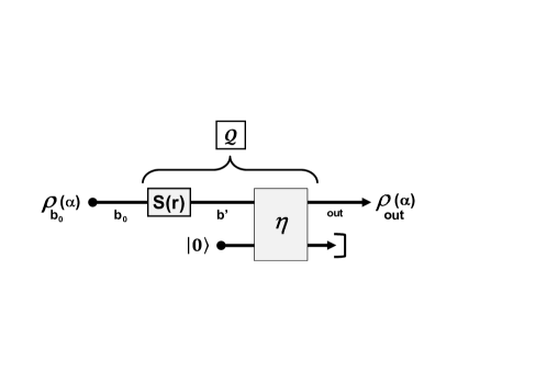
Figure 14: Decomposition of Bob’s quantum operation $\mathcal{Q}$ into a single-mode squeezer $S(r)$ followed by an amplifying channel $\mathcal{A}(\eta)$, which can be dilated into a two-mode squeezer involving a vacuum input.

The action of the squeezer is to balance the diagonal terms in Eq. (63), so that the position and momentum components are equal. This corresponds to apply a symplectic squeezing matrix

$$\mathbf{S}(r)=\left(\begin{array}[c]{cc}r&0\\ 0&\frac{1}{r}\end{array}\right)~{}\text{with}~{}r=\sqrt{\frac{\theta_{1}}{\theta_{1}^{\prime}}},$$ (64)

so that we have

$$\mathbf{\bar{x}}_{b^{\prime}|\alpha}:=\mathbf{S}(r)~{}\mathbf{\bar{x}}_{b_{0}|\alpha}=\frac{\tau\tilde{\mu}}{2\sqrt{\theta_{1}\theta_{1}^{\prime}}}~{}\mathbf{\bar{x}}_{A|\alpha}.$$

Now, we apply a phase-insensitive quantum-limited amplifier, i.e., a two-mode squeezer combining the state with a vacuum state. This device realizes an amplifying channel transforming the quadrature operators $\mathbf{\hat{x}}=(\hat{q},\hat{p})^{T}$ as

$$\mathbf{\hat{x}}_{b^{\prime}|\alpha}\rightarrow\mathbf{\hat{x}}_{\text{out}|\alpha}=\sqrt{\eta}\mathbf{\hat{x}}_{b^{\prime}|\alpha}+\sqrt{\eta-1}\mathbf{Z\hat{x}}_{\text{vac}},$$

where $\mathbf{\hat{x}}_{\text{vac}}$ are the quadrature operators of the vacuum mode. Choosing the gain to be

$$\eta=\frac{4\theta_{1}\theta_{1}^{\prime}}{\tau^{2}(\mu^{2}-1)}\geq 1,$$ (65)

we have that the output state has the desired mean value

$$\mathbf{\bar{x}}_{\text{out}|\alpha}=\sqrt{\eta}\mathbf{\bar{x}}_{b^{\prime}|\alpha}=\mathbf{\bar{x}}_{A|\alpha}.$$

It is clear that such quantum processing by $\mathcal{Q}$ does not come for free. Recovering the mean-value of the input coherent state is achieved at the cost of increasing the noise in the teleported state. In fact, the CM of the output state $\rho_{\text{out}}(\alpha)$ is given by

$$\mathbf{V}_{\text{out}|\alpha}=\eta\left[\mathbf{S}(r)\mathbf{V}_{b_{0}|\alpha}\mathbf{S}(r)^{T}\right]+(\eta-1)\mathbf{I~{}.}$$ (66)

Using Eqs. (54), (64) and (65) in Eq. (66), we get

$$\mathbf{V}_{\text{out}|\alpha}=\frac{4\mu}{\tau^{2}(\mu^{2}-1)}\left(\begin{array}[c]{cc}\theta_{1}^{2}&0\\ 0&\theta_{1}^{\prime 2}\end{array}\right)-\frac{2}{\tau}\left(\begin{array}[c]{cc}\theta_{1}&0\\ 0&\theta_{1}^{\prime}\end{array}\right)+(\eta-1)\mathbf{I}.$$

Once we have derived its the first and second-order statistical moments, the teleported Gaussian state $\rho_{\text{out}}(\alpha)$ is fully determined. For a given outcome $\alpha$, the fidelity of teleportation

$$F(\alpha)=\mathrm{Tr}\left[\left|\nu(\alpha)\right\rangle\left\langle\nu(\alpha)\right|\rho_{\text{out}}(\alpha)\right]$$

can be computed using the trace-rule for Gaussian states. In general, for two arbitrary single-mode Gaussian states, $\rho$ and $\rho^{\prime}$, with statistical moments $\{\mathbf{\bar{x}},\mathbf{V}\}$ and $\{\mathbf{\bar{x}}^{\prime},\mathbf{V}^{\prime}\}$, we can write

$$\mathrm{Tr}\left(\rho\rho^{\prime}\right)=\frac{2\exp\left[-\frac{1}{2}(\mathbf{\bar{x}-\bar{x}}^{\prime})^{T}(\mathbf{V}+\mathbf{V}^{\prime})^{-1}(\mathbf{\bar{x}-\bar{x}}^{\prime})\right]}{\sqrt{\det(\mathbf{V}+\mathbf{V}^{\prime})}}.$$

Applying this formula to our specific case, we obtain $F(\alpha)=2N^{-1}$, where

$$N :=\sqrt{\det(\mathbf{V}_{\text{out}|\alpha}+\mathbf{I})}$$

$$=\frac{2\sqrt{\theta_{1}\theta_{1}^{\prime}}}{\tau}\sqrt{\frac{2(\mu\theta_{1}+\theta_{1}^{\prime})}{\tau(\mu^{2}-1)}-1}\sqrt{\frac{2(\mu\theta_{1}^{\prime}+\theta_{1})}{\tau(\mu^{2}-1)}-1}$$

$$=\frac{2}{\mu^{2}-1}\sqrt{(1+\mu+2\kappa)(1+\mu+2\kappa^{\prime})}\times$$

$$\sqrt{1+\kappa^{\prime}+\mu(1+\kappa)}\sqrt{1+\kappa+\mu(1+\kappa^{\prime})}~{}.$$

Since input and output states have the same mean-value, $F(\alpha)$ is constant in $\alpha$, so that it coincides with the average teleportation fidelity of Eq. (53), i.e., we find

$$F=\frac{2}{N}:=F(\mu,\kappa,\kappa^{\prime}).$$ (67)

Besides $\mu$, this is clearly a function of the environmental parameters ($\tau$, $\omega$, $g$ and $g^{\prime}$) via $\kappa$ and $\kappa^{\prime}$. We can then fix an experimentally achievable value for $\mu$ (in particular, $\mu\simeq 6.5$, corresponding to about 11dB of two-mode squeezing dB ; TopENT ; TobiasSqueezing ), and consider an environment with transmissivity $\tau$ and entanglement-breaking thermal noise $\omega>\omega_{\text{EB}}(\tau)$. We can therefore explore the points in the correlation plane $(g,g^{\prime})$ where the protocol is quantum, i.e., $F>1/2$. This is done in Fig. 4 of the main text.

One can easily check that the average teleportation fidelity of Eq. (67) is an increasing function in the parameter $\mu$, as clearly expected since this parameter quantifies the amount of entanglement in Bob’s TMSV state. The average teleportation fidelity is therefore maximum in the limit $\mu\gg 1$. At the leading order in $\mu$, we derive the asymptotic expression

$$F=F_{\text{opt}}+O(\mu^{-1}),~{}~{}F_{\text{opt}}=\frac{1}{\sqrt{(1+\kappa)(1+\kappa^{\prime})}},$$ (68)

where $\kappa$ and $\kappa^{\prime}$ are given in Eq. (41). It is easy to check that the fidelity in Eq. (68) may be written as

$$F_{\text{opt}}=\frac{1}{\sqrt{1+\varepsilon_{\text{opt}}^{2}+\Omega}},$$

where

$$\Omega:=\kappa+\kappa^{\prime}=(\tau^{-1}-1)(2\omega+g^{\prime}-g),$$ (69)

and $\varepsilon_{\text{opt}}=\sqrt{\kappa\kappa^{\prime}}$ is the asymptotic PTS eigenvalue of Eq. (52). This eigenvalue quantifies the amount of entanglement which would be shared by Alice and Bob if we replaced the teleportation protocol with an entanglement swapping protocol, where Alice has the same TMSV state as Bob ($\varphi=\mu\gg 1$) and receives the classical communication from Charlie.

Note that, since $\Omega\geq 2\varepsilon_{\text{opt}}$, we have the upper-bound

$$F_{\text{opt}}\leq\frac{1}{1+\varepsilon_{\text{opt}}},$$ (70)

with the equality $F=(1+\varepsilon_{\text{opt}})^{-1}$ holding for environments with antisymmetric correlations $g+g^{\prime}=0$ (in fact this implies $\kappa=\kappa^{\prime}$ and therefore $\Omega=2\varepsilon_{\text{opt}}$). Thus, in these antisymmetric environments, we have a full equivalence between the asymptotic protocols of quantum teleportation and entanglement swapping: Teleportation of coherent states is quantum ($F_{\text{opt}}>1/2$) if and only if CV entanglement is swapped ($\varepsilon_{\text{opt}}<1$).

Sec. 2.7 Distillation

Sec. 2.7.1 Entanglement Distillation

Entanglement distillation can be operated on top of entanglement swapping. After the parties have run the swapping protocol many times and stored their remote modes in quantum memories, they can perform a one-way entanglement distillation protocol on the whole set of swapped states. This consists of Alice locally applying an optimal quantum instrument QinstNOTE $\mathcal{A}$ on her modes $a$, whose quantum outcome $\boldsymbol{\alpha}$ is a distilled system while the classical outcome $k$ is communicated. Upon receipt of $k$, Bob performs a conditional quantum operation $\mathcal{B}_{k}$ transforming his modes $b$ into a distilled system $\boldsymbol{\beta}$ (see Fig. 15 for a schematic).

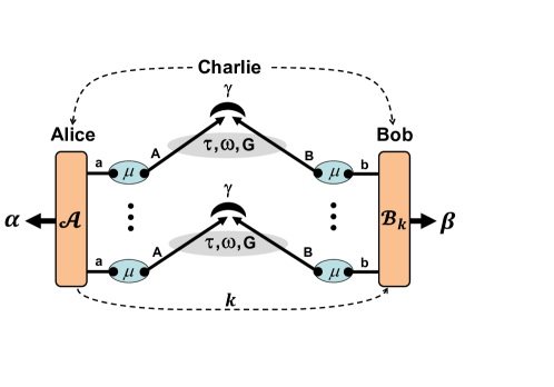
Figure 15: Entanglement distillation protocol based on one-way classical communication. This is operated on top of entanglement swapping to realize a non-Gaussian quantum repeater. See text for details.

The process can be designed to be highly non-Gaussian so that the distilled systems have discrete variables and are collapsed into a number of entanglement bits (Bell state pairs). According to the hashing inequality Qinstrument , the distillation rate achievable by one-way distillation protocols is lower bounded by the coherent information CohINFO ; CohINFO2 . In general, the coherent information of a bipartite state $\rho_{ab}$ is defined as

$$I_{\mathcal{C}}(\rho_{ab}):=S(\rho_{b})-S(\rho_{ab})~{},$$

where $\rho_{b}=\mathrm{Tr}_{a}(\rho_{ab})$ and $S(\rho):=-$Tr$(\rho\log_{2}\rho)$ is the von Neumann entropy. This is also denoted by $I(a\rangle b)$. In particular, the coherent information of a two-mode Gaussian state $\rho_{ab}$ depends only on its CM

$$\mathbf{V}=\left(\begin{array}[c]{cc}\mathbf{A}&\mathbf{C}\\ \mathbf{C}^{T}&\mathbf{B}\end{array}\right).$$

In fact, it can be written as

$$I_{\mathcal{C}}(\rho_{ab})=h(\nu_{b})-h(\nu_{-})-h(\nu_{+})~{},$$ (71)

where the entropic function RMP

$$h(x):=\frac{x+1}{2}\log_{2}\left(\frac{x+1}{2}\right)-\frac{x-1}{2}\log_{2}\left(\frac{x-1}{2}\right)$$ (72)

is applied to $\nu_{b}=\sqrt{\det\mathbf{B}}$ (symplectic eigenvalue of $\mathbf{B}$) and $\{\nu_{-},\nu_{+}\}$, which is the symplectic spectrum of $\mathbf{V}$. In the specific case where all symplectic eigenvalues are large, we can use the expansion

$$h(x)=\log_{2}\left(\frac{ex}{2}\right)+O\left(x^{-1}\right)~{}~{}(x\gg 1)~{},$$ (73)

which leads to the following asymptotic formula

$$I_{\mathcal{C}}(\rho_{ab})\simeq\log_{2}\left(\frac{2}{e}\sqrt{\frac{\det\mathbf{B}}{\det\mathbf{V}}}\right)~{}.$$ (74)

In our analysis, the coherent information $I_{\mathcal{C}}$ has to be computed on the swapped state $\rho_{ab|\gamma}$ whose CM is given in Eqs. (42), (45) and (48). It is clear that $I_{\mathcal{C}}(\rho_{ab|\gamma})$ does not depend on the specific value of the outcome $\gamma$ (for Gaussian states, the von Neumann entropy and the coherent information do not depend on the first statistical moments, which are those encoding the specific value $\gamma$ of the Bell detection). By replacing the symplectic eigenvalues in Eqs. (49) and (50) into Eq. (71), we derive a closed analytical expression for $I_{\mathcal{C}}(\rho_{ab|\gamma})$ as function of the main parameters of the problem. Explicitly, we have

$$I_{\mathcal{C}}(\rho_{ab|\gamma}) =h\left[\frac{1}{2}\sqrt{\frac{(1+2\mu\kappa+\mu^{2})(1+2\mu\kappa^{\prime}+\mu^{2})}{(\mu+\kappa)(\mu+\kappa^{\prime})}}\right]$$

$$-h\left[\sqrt{\frac{\mu(1+\mu\kappa)}{\mu+\kappa}}\right]-h\left[\sqrt{\frac{\mu(1+\mu\kappa^{\prime})}{\mu+\kappa^{\prime}}}\right]$$

$$:=I_{\mathcal{C}}(\mu,\tau,\omega,g,g^{\prime}).$$ (75)

This quantity can numerically be studied considering low values of the parameter $\mu$, i.e., for experimentally achievable values of the input entanglement (in particular, $\mu\simeq 6.5$). As we show in Fig. 4 of the main text, entanglement distillation is possible in the presence of entanglement-breaking channels as long as sufficient amount of separable correlations is present in the non-Markovian Gaussian environment.

As one intuitively expects and can easily verify via the computation of the derivatives, the coherent information of Eq. (75) is increasing for increasing $\mu$, reaching its optimal value for large input entanglement ($\mu\gg 1$). The spectra of the two Gaussian states $\rho_{ab|\gamma}$ and $\rho_{b|\gamma}$ are both diverging in $\mu$, as one can check directly from the CM $\mathbf{V}_{ab|\gamma}$ and the reduced CM $\mathbf{V}_{b|\gamma}$, which is just the block $\mathbf{B}$ in Eq. (45). For large $\mu$, we find

$$\det\mathbf{B}\simeq\mu^{2}/4,~{}\det\mathbf{V}_{ab|\gamma}\simeq(\varepsilon_{\text{opt}}\mu)^{2}~{},$$

where $\varepsilon_{\text{opt}}$ is the asymptotic expression of the smallest PTS eigenvalue given in Eq. (52). Thus, using Eq. (74), we find the following asymptotic expression for the coherent information

$$I_{\mathcal{C}}(\rho_{ab|\gamma})\simeq I_{\mathcal{C}\text{,opt}}:=-\log_{2}\left(e\varepsilon_{\text{opt}}\right)~{},$$

which is the one given in the main text. Asymptotically in the input resources, we have that entanglement can be distilled ($I_{\mathcal{C}\text{,opt}}>0$) for $\varepsilon_{\text{opt}}<e^{-1}\simeq 0.367$. Such condition is more demanding to be satisfied with respect to that of simple entanglement swapping ($\varepsilon_{\text{opt}}<1$), so that it requires the presence of more separable correlations in the environment, as shown by Fig. 4 in the main text.

Finally, we remark that what we computed is the rate achievable by one-way coherent protocols operated on top of entanglement swapping, i.e., after a large amount of swapped states are available in Alice’s and Bob’s quantum memories. It is interesting to note that this approach seems to be more robust than the other one where the two procedures are inverted (so that sessions of entanglement distillation are performed with the relay, followed by entanglement swapping on the distilled states). In a correlated Gaussian environment with entanglement-breaking noise, we have that ‘swapping plus distillation’ can work, while ‘distillation plus swapping’ tends to fail if the environmental correlations are washed out during the distillation stage.

Sec. 2.7.2 Secret-Key Distillation

The previous one-way entanglement distillation protocol of Fig. 15 can be modified into a one-way key distillation protocol, where Charlie is a generally-untrusted relay distributing secret correlations to Alice and Bob. Despite the fact that Charlie could be played by an eavesdropper (Eve), the action of the Bell detection does not give Eve any information. Furthermore, if Eve tries to tamper with the working mechanism of the relay, Alice and Bob can always undo this action on the relay and absorb its effects in the environment. This is a key point of measurement-device-independent (MDI) QKD mdiQKD ; Untrusted .

The environment must be interpreted as the effect of a coherent attack of the eavesdropper. This can be reduced to a two-mode coherent attack within each single use of the relay (by adopting quantum de Finetti arguments) and, in particular, to a two-mode Gaussian attack, by using the extremality of Gaussian states Untrusted . In such a Gaussian attack, Eve’s output modes $\mathbf{E}$ (not shown in the figure) are stored in a quantum memory and finally detected. Alice’s quantum instrument $\mathcal{A}$ is here a quantum measurement with classical outputs $\boldsymbol{\alpha}$ (the secret key) and $k$ (assisting data for Bob). Bob’s operation $\mathcal{B}_{k}$ is a coherent measurement conditioned on $k$, which provides the classical output $\boldsymbol{\beta}$ (key estimate).

This is an ideal key distribution protocol KeyCAP whose rate $K$ is lower-bounded by the Devetak-Winter rate $R_{\text{DW}}$ DW ; SciREP . In fact, let us restrict Alice to individual measurements, each one applied to one mode $a$ with outcome $\alpha$. Then, we can write

$$K\geq R_{\text{DW}}=\chi_{ab|\gamma}-\chi_{a\mathbf{E}|\gamma}~{},$$ (76)

where $\chi_{ab(\mathbf{E})|\gamma}$ is the conditional Holevo information between mode $a$ and mode $b$ (modes $\mathbf{E}$). Explicitly,

$$\chi_{ab|\gamma} =S(\rho_{b|\gamma})-S(\rho_{b|\gamma\alpha})~{},$$ (77)

$$\chi_{a\mathbf{E}|\gamma} =S(\rho_{\mathbf{E}|\gamma})-S(\rho_{\mathbf{E}|\gamma\alpha})~{},$$ (78)

where $\rho_{b|\gamma}$ ($\rho_{\mathbf{E}|\gamma}$) is the conditional state of Bob (Eve) after each use of the relay, and $\rho_{b|\gamma\alpha}$ ($\rho_{\mathbf{E}|\gamma\alpha}$) is the corresponding projected state for Bob (Eve) after Alice’s further measurement, with outcome $\alpha$.

Note that the Bell detection is a rank-1 measurement, therefore projecting pure states into pure states. For this reason we have that the global state $\rho_{ab\mathbf{E}|\gamma}$ is pure and therefore

$$S(\rho_{\mathbf{E}|\gamma})=S(\rho_{ab|\gamma})~{}.$$ (79)

If we now restrict Alice’s individual measurements to be rank-1, then we also have that $\rho_{b\mathbf{E}|\gamma\alpha}$ is pure, so that

$$S(\rho_{\mathbf{E}|\gamma\alpha})=S(\rho_{b|\gamma\alpha})~{}.$$ (80)

Thus, using Eqs. (77)-(80), we may write

$$R_{\text{DW}}\geq R_{\text{DW}}^{\text{rank-1}}=S(\rho_{b|\gamma})-S(\rho_{ab|\gamma})=I_{\mathcal{C}}(\rho_{ab|\gamma}).$$ (81)

Combining Eqs. (76) and (81), we finally achieve

$$K\geq I_{\mathcal{C}}(\rho_{ab|\gamma}),$$

which is the result stated in the main text.

Sec. 2.8 Relay-based practical QKD

Sec. 2.8.1 Description and security analysis

The previous ideal key-distillation protocol can be simplified by removing quantum memories and using one-mode measurements for the parties, in particular, heterodyne detections. This becomes the entanglement-based representation of an equivalent ‘prepare and measure’ protocol where amplitude-modulated coherent states ($\left|\tilde{\alpha}\right\rangle$ on Alice’s mode $A$, and $|\tilde{\beta}\rangle$ on Bob’s mode $B$) are prepared and sent to the relay (see Fig. 16). In particular, the values of the amplitudes are simply connected with the outcomes of the heterodyne detectors in the equivalent entanglement-based representation. The amplitudes satisfy the relations

$$\left(\begin{array}[c]{c}\tilde{\alpha}\\ \tilde{\beta}\end{array}\right)=\frac{\sqrt{\mu^{2}-1}}{\mu+1}\left(\begin{array}[c]{c}\alpha^{\ast}\\ \beta^{\ast}\end{array}\right),$$

where $\alpha$ and $\beta$ are the outcomes of the virtual heterodyne detectors and $\mu$ is the variance of the virtual TMSV states at Alice’s and Bob’s stations. As a result the amplitudes $\tilde{\alpha}$ and $\tilde{\beta}$ of the coherent states are Gaussianly modulated with a variance $\mu-1$ (see Ref. HET and also the Supplementary Material of Ref. OptimalDiscord ).

At the relay the transmitted states are subject to Bell detection and the result $\gamma$ is communicated back to the parties. Since $\gamma\simeq\alpha-\beta^{\ast}$, we have that classical correlations are remotely created between Alice’s and Bob’s complex variables. As mentioned before, the knowledge of $\gamma$ alone does not help Eve as long as the variance of the modulation $\mu-1$ is sufficiently high. Experimentally, values of modulation $\mu\gtrsim 50$ are easily achievable and already well approximate the performance of the asymptotic scenario $\mu\gg 1$ (in terms of secret key rate assuming ideal reconciliation performances).

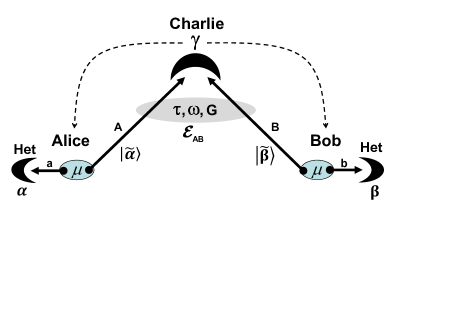
Figure 16: Entanglement-based representation of a practical QKD protocol where coherent states are prepared and sent to Charlie for Bell detection. Charlie is an untrusted relay, meaning that he could be Eve (relay is an MDI-QKD node).

The non-Markovian environment is the result of Eve’s attack. Eve stores all her output ancillas $\mathbf{E}$ (not shown) in a quantum memory which is subject to a final optimized coherent measurement. As previously discussed, this environment may also absorb the effects of an attack directed at the working mechanism of the middle relay. Furthermore, suitable classes of side-channel attacks which directly affect the optical preparations inside Alice’s and Bob’s private spaces can also be treated as part of the external environment.

Despite the fact that the protocol is performed as a prepare and measure protocol, its security is more easily studied considering its entanglement-based representation. In this equivalent representation, Alice and Bob can estimate the post-relay conditional quantum state $\rho_{ab|\gamma}$ by comparing a subset of their data and analyzing the joint classical statistics $p(\tilde{\alpha},\tilde{\beta},\gamma)$. Then, Alice and Bob purify $\rho_{ab|\gamma}$ into an environment $\mathbf{E}$ which is fully controlled by Eve. In these general conditions, the two parties are able to compute the secret key rate directly from the CM $\mathbf{V}_{ab|\gamma}$ of $\rho_{ab|\gamma}$. Because of the extremality properties of Gaussian states, Alice and Bob can always assume that $\rho_{ab|\gamma}$ is Gaussian Untrusted .

Let us discuss in detail how the rate of the protocol can be computed from the second-order statistical moments $\mathbf{V}_{ab|\gamma}$. After the action of the relay, Alice and Bob’s mutual information

$$I_{AB|\gamma}:=I(\tilde{\alpha}:\tilde{\beta}|\gamma)=I(\alpha:\beta|\gamma)$$

is given by Untrusted

$$I_{AB|\gamma}=\frac{1}{2}\log_{2}\Sigma,~{}~{}\Sigma:=\frac{1+\det\mathbf{V}_{b|\gamma}+\mathrm{Tr}\mathbf{V}_{b|\gamma}}{1+\det\mathbf{V}_{b|\gamma\alpha}+\mathrm{Tr}\mathbf{V}_{b|\gamma\alpha}}.$$ (82)

Here $\mathbf{V}_{b|\gamma}$ is the CM of Bob’s reduced state $\rho_{b|\gamma}$ and $\mathbf{V}_{b|\gamma\alpha}$ is the CM of Bob’s state $\rho_{b|\gamma\alpha}$ after the detections of both the relay and Alice. The latter CM can easily be computed from the CM $\mathbf{V}_{ab|\gamma}$ using the formulas for the heterodyne detection HET .

To bound Eve’s stolen information on Alice’s variable $\alpha$, we use the conditional Holevo information $\chi_{a\mathbf{E}|\gamma}$ between Alice’s (detected) mode $a$ and Eve’s output ancillas $\mathbf{E}$ for the single use of the relay. Since the Bell detection at the relay is rank-1, the conditional global state $\rho_{ab\mathbf{E}|\gamma}$ of Alice, Bob and Eve is pure. Furthermore, Alice’s heterodyne detection is also rank-1, so that the double-conditional state $\rho_{b\mathbf{E}|\gamma\alpha}$ is also pure. This means that we can exploit the entropic equalities $S(\rho_{\mathbf{E}|\gamma})=S(\rho_{ab|\gamma})$ and $S(\rho_{\mathbf{E}|\gamma\alpha})=S(\rho_{b|\gamma\alpha})$. Thus, we may write

$$\chi_{a\mathbf{E}|\gamma}=S(\rho_{ab|\gamma})-S(\rho_{b|\gamma\alpha}).$$ (83)

This quantity can be computed from the symplectic spectra of the CMs $\mathbf{V}_{ab|\gamma}$ and $\mathbf{V}_{b|\gamma\alpha}$. We have

$$\chi_{a\mathbf{E}|\gamma}=h(\nu_{-})+h(\nu_{+})-h(\nu_{\text{c}}),$$ (84)

where the function $h(x)$ of Eq. (72) is applied to the symplectic spectrum $\{\nu_{-},\nu_{+}\}$ of $\mathbf{V}_{ab|\gamma}$ and $\nu_{\text{c}}=\sqrt{\det\mathbf{V}_{b|\gamma\alpha}}$.

The secret key rate is finally given by the difference

$$R=\xi I_{AB|\gamma}-\chi_{a\mathbf{E}|\gamma}$$ (85)

where $\xi\leq 1$ is the reconciliation efficiency (due to the finite efficiency of realistic codes for error correction and privacy amplification). Thus, the rate can be computed from the second-order moments, in particular, from $\mathbf{V}_{ab|\gamma}$. This procedure is very general: In the next section it is used to derive the analytical expression of the key rate from the main parameters of a two-mode Gaussian attack against the two links; afterwards, in Sec. 4, it is used to derive the experimental key rate from the statistics of the shared classical data.

Sec. 2.8.2 Analytical expression of the key rate

Let us consider a two-mode Gaussian attack of the links which results into a non-Markovian Gaussian environment with correlated-thermal noise, with parameters $\tau$, $\omega$, $g$ and $g^{\prime}$, as described in Sec. 2.1. Then, the conditional CM $\mathbf{V}_{ab|\gamma}$ is specified by Eqs. (42)-(48). Bob’s reduced CM $\mathbf{V}_{b|\gamma}$ is the block $\mathbf{B}$ given in Eq. (45). The expression of $\mathbf{V}_{b|\gamma\alpha}$ has been already obtained in Eqs. (54)-(56). Thus, for Alice and Bob’s mutual information $I_{AB|\gamma}$, we find

$$\Sigma=\frac{\left(1+\mu+2\kappa\right)^{2}\left(1+\mu+2\kappa^{\prime}\right)^{2}}{16(1+\kappa)(1+\kappa^{\prime})(\mu+\kappa)(\mu+\kappa^{\prime})}~{}.$$

For the computation of Eve’s Holevo information $\chi_{a\mathbf{E}|\gamma}$, we see that the symplectic spectrum $\{\nu_{-},\nu_{+}\}$ of $\mathbf{V}_{ab|\gamma}$ is given in Eq. (49), and we compute

$$\nu_{\text{c}}=\sqrt{\frac{\left(1+\mu+2\mu\kappa\right)\left(1+\mu+2\mu\kappa^{\prime}\right)}{\left(1+\mu+2\kappa\right)\left(1+\mu+2\kappa^{\prime}\right)}}~{}.$$

The rate is an analytical but cumbersome function of the relevant parameters of the problem, i.e., the finite reconciliation efficiency $\xi$, the signal modulation variance $\mu$ of the coherent states, and the $\kappa$-parameters of the environment. Explicitly, we have

$$R =\frac{\xi}{2}\log_{2}\frac{\left(1+\mu+2\kappa\right)^{2}\left(1+\mu+2\kappa^{\prime}\right)^{2}}{16(1+\kappa)(1+\kappa^{\prime})(\mu+\kappa)(\mu+\kappa^{\prime})}$$

$$-h\left[\sqrt{\frac{\mu(1+\mu\kappa)}{\mu+\kappa}}\right]-h\left[\sqrt{\frac{\mu(1+\mu\kappa^{\prime})}{\mu+\kappa^{\prime}}}\right]$$

$$+h\left[\sqrt{\frac{\left(1+\mu+2\mu\kappa\right)\left(1+\mu+2\mu\kappa^{\prime}\right)}{\left(1+\mu+2\kappa\right)\left(1+\mu+2\kappa^{\prime}\right)}}\right]$$

$$:=R(\xi,\mu,\kappa,\kappa^{\prime})$$ (86)

Using the expressions for the $\kappa$-parameters in Eq. (41), we can write the rate as $R=R(\xi,\mu,\tau,\omega,g,g^{\prime})$, i.e., directly in terms of the parameters of the two-mode Gaussian attack, i.e., the transmissivity $\tau$, the variance of the thermal noise $\omega$ and the correlation parameters $g$ and $g^{\prime}$. Fixing the reconciliation efficiency (e.g., to be ideal $\xi=1$ or achievable $\xi\simeq 0.97~{}$Jouguetapp ) and the modulation $\mu\simeq 50$, we can study the rate $R$ in an entanglement-breaking Gaussian attack with $\tau=0.9$ and $\omega=(1+10^{-4})\omega_{\text{EB}}\simeq 19$ (about 9 thermal photons). The security threshold $R=0$ can be plotted in the correlation plane $(g,g^{\prime})$ as shown in Fig 17.

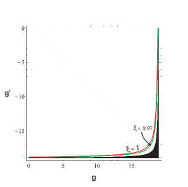
Figure 17: Security thresholds $R=0$ in the correlation plane, considering $\mu\simeq 50$ and $\xi=1$ (red line) and $\xi\simeq 0.97$ (green line). Below the thresholds the corresponding rates are positive. Other parameters are $\tau=0.9$ and $\omega\simeq 19>\omega_{\text{EB}}.$

As we can see from Fig. 17, the secret-key rate can be positive for sufficiently high separable correlations in the Gaussian attack. Furthermore, there is no much difference between the cases with ideal ($\xi=1$) or achievable ($\xi\simeq 0.97$) reconciliation efficiency. For this reason, in the theoretical discussions of the main text we have only considered the simpler case of ideal reconciliation, i.e., the rate $R=R(1,\mu,\kappa,\kappa^{\prime})=R(1,\mu,\tau,\omega,g,g^{\prime})$.

In order to show the optimal performance of the QKD protocol, we consider ideal reconciliation ($\xi=1$) and we perform the limit of large modulation $\mu\gg 1$ (in fact, by assuming ideal reconciliation, the rate is increasing in $\mu$). Let us derive the asymptotic optimal rate

$$R(1,\mu\gg 1,\kappa,\kappa^{\prime})\simeq R_{\text{opt}}(\kappa,\kappa^{\prime})=R_{\text{opt}}(\tau,\omega,g,g^{\prime}).$$

At the leading order in $\mu$, we find

$$\Sigma =\frac{\mu^{2}}{16(1+\kappa)(1+\kappa^{\prime})}+O(\mu),$$ (87)

$$\nu_{\text{c}} =\sqrt{(1+2\kappa)(1+2\kappa^{\prime})}+O(\mu^{-1}),$$ (88)

$$\nu_{-} =\sqrt{\kappa\mu}+O(\mu^{-1/2}),$$ (89)

$$\nu_{+} =\sqrt{\kappa^{\prime}\mu}+O(\mu^{-1/2}),$$ (90)

where $\kappa$ and $\kappa^{\prime}$ are given in Eq. (41). Using the previous Eqs. (87)-(90) and the expansion in Eq. (73) we find the simple formula

$$R_{\text{opt}} =\log_{2}\left[\frac{1}{e^{2}\sqrt{(1+\kappa)(1+\kappa^{\prime})\kappa\kappa^{\prime}}}\right]$$

$$+h\left[\sqrt{(1+2\kappa)(1+2\kappa^{\prime})}\right].$$

We can easily connect this asymptotic key rate with the asymptotic PTS eigenvalue $\varepsilon_{\text{opt}}$ of Eq. (52) and the asymptotic fidelity $F_{\text{opt}}$ of Eq. (68). In fact, we may write

$$R_{\text{opt}}=\log_{2}\left(\frac{F_{\text{opt}}}{e^{2}\varepsilon_{\text{opt}}}\right)+h\left[\sqrt{1+(2\varepsilon_{\text{opt}})^{2}+2\Omega}\right]$$ (91)

where we have also used $\Omega:=\kappa+\kappa^{\prime}\geq 2\varepsilon_{\text{opt}}$. Using the latter inequality, we may write the lower bound

$$R_{\text{opt}}\geq R_{\text{LB}}:=\log_{2}\left(\frac{F_{\text{opt}}}{e^{2}\varepsilon_{\text{opt}}}\right)+h(1+2\varepsilon_{\text{opt}}).$$ (92)

As we can see from Fig. 18, this bound is sufficiently tight for the most interesting range of parameters, i.e., for environments with antisymmetric correlations $g+g^{\prime}\simeq 0$ (around the diagonal of the correlation plane). In particular, for environments with exactly $g+g^{\prime}=0$, we have the equality

$$R_{\text{opt}}=R_{\text{LB}}=\log_{2}\left[\frac{1}{e^{2}\varepsilon_{\text{opt}}(1+\varepsilon_{\text{opt}})}\right]+h(1+2\varepsilon_{\text{opt}}),$$ (93)

since we have $\kappa=\kappa^{\prime}$ which implies both $\Omega=2\varepsilon_{\text{opt}}$ and $F_{\text{opt}}=(1+\varepsilon_{\text{opt}})^{-1}$.

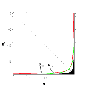
Figure 18: Security thresholds $R_{\text{opt}}=0$ (red line) and $R_{\text{LB}}=0$ (green line). Other parameters are $\tau=0.9$ and $\omega\simeq 19>\omega_{\text{EB}}$.

Note that the left hand sides of Eqs. (92) and (93) can be positive only for $\varepsilon_{\text{opt}}\lesssim 0.192$. Asymptotically, the practical QKD protocol appears to be the most difficult to reactivate: Its reactivation implies that of entanglement/key distillation ($\varepsilon_{\text{opt}}<0.367$) and that of entanglement swapping ($\varepsilon_{\text{opt}}<1$).

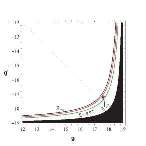
Figure 19: Comparison between $R_{\text{opt}}=0$ (black line), $R=0$ with $\mu\simeq 50$ and $\xi=1$ (red line), and $R=0$ with $\mu\simeq 50$ and $\xi=0.97$ (green line). Other parameters are $\tau=0.9$ and $\omega\simeq 19>\omega_{\text{EB}}$.

In conclusion, we also show that the asymptotic key rate $R_{\text{opt}}$ is well approximated by the finite modulation rate $R$ with $\mu\simeq 50$ (assuming both the case of ideal reconciliation $\xi=1$ and realistic reconciliation efficiency $\xi\simeq 0.97$). This is evident from Fig. 19, which is a zoom on the most interesting part of the correlation plane. We see that considering realistic finite modulations and reconciliation efficiencies does not sensibly degrade the reactivation process (determined by the performances of the various security thresholds).

Sec. 3 Theory: Correlated-Additive Noise

Here we extend our previous analysis to another kind of non-Markovian environment, which is the Gaussian environment with correlated-additive noise. Here we provide full details on the following theoretical elements:

$\bullet~{}$SSec. 3.1: We show how the correlated-additive environment can be obtained as a suitable limit of the previous correlated-thermal environment.

$\bullet~{}$Sec. 3.2: We derive the CM of the swapped state in this environment. We discuss the condition for swapping reactivation, and we identify optimal and suboptimal points for reactivation.

$\bullet~{}$Sec. 3.3: We study the security of the practical relay-based QKD protocol, providing the general formula for its secret-key rate $R(\xi,\mu,n,c,c^{\prime})$. We then discuss the reactivation of this practical protocol from entanglement-breaking.

Sec. 3.1 Additive-Noise Limit

The correlated-additive Gaussian environment can be obtained from the previous correlated-thermal Gaussian environment by taking a suitable continuous limit (where the continuity is guaranteed by the Gaussian nature of all the process). In particular, we consider the limit for $\tau\rightarrow 1$ and $\omega\rightarrow+\infty$, while keeping constant

$$n:=(1-\tau)\omega,~{}c:=\frac{g}{\omega-1},~{}c^{\prime}:=\frac{g^{\prime}}{\omega-1}.$$ (94)

The effect of this limit can be understood studying the CM of the modes $A^{\prime}$ and $B^{\prime}$ after the action of the channel and before the Bell detection. For the correlated-thermal Gaussian environment, we have the following CM

$$\mathbf{V}_{A^{\prime}B^{\prime}}=\left(\begin{array}[c]{cc}[\tau\mu+(1-\tau)\omega]\mathbf{I}&(1-\tau)\mathbf{G}\\ (1-\tau)\mathbf{G}&[\tau\mu+(1-\tau)\omega]\mathbf{I}\end{array}\right),$$ (95)

which can easily be derived from Eq. (35) by setting $\varphi=\mu$ and deleting the entries of modes $a$ and $b$. Now taking the previous limit, it leads to

$$\mathbf{V}_{A^{\prime}B^{\prime}}\rightarrow\mathbf{V}_{A^{\prime}B^{\prime}}^{\text{add}}=\left(\begin{array}[c]{cc}(\mu+n)\mathbf{I}&n\mathbf{C}\\ n\mathbf{C}&(\mu+n)\mathbf{I}\end{array}\right),$$ (96)

where

$$\mathbf{C}:=\left(\begin{array}[c]{cc}c&0\\ 0&c^{\prime}\end{array}\right),$$

and we have used $(1-\tau)\mathbf{G}=(1-\tau)(\omega-1)\mathbf{C}\rightarrow n\mathbf{C}$.

As we can easily check, the CM in Eq. (96) can be decomposed as follows

$$\mathbf{V}_{A^{\prime}B^{\prime}}^{\text{add}}=\mathbf{V}_{AB}+n\left(\begin{array}[c]{cc}\mathbf{I}&\mathbf{C}\\ \mathbf{C}&\mathbf{I}\end{array}\right),$$

so that the environment adds classical Gaussian noise to the input CM $\mathbf{V}_{AB}=\mu(\mathbf{I}\oplus\mathbf{I})$ with variance $n\geq 0$ in each quadrature, and noise-correlations described by the off-diagonal block $n\mathbf{C}$, with parameters $-1\leq c,c^{\prime}\leq 1$.

In terms of input-output quadrature transformations, the action of the asymptotic environment is therefore described by

$$\left\{\begin{array}[c]{c}\hat{q}_{A^{\prime}}=\hat{q}_{A}+\xi_{1},\\ \hat{p}_{A^{\prime}}=\hat{p}_{A}+\xi_{2},\\ \hat{q}_{B^{\prime}}=\hat{q}_{B}+\xi_{3},\\ \hat{p}_{B^{\prime}}=\hat{p}_{B}+\xi_{4},\end{array}\right.$$ (97)

where the $\xi_{i}$’s are zero-mean Gaussian variables whose covariances $\left\langle\xi_{i}\xi_{j}\right\rangle$ are given by the classical CM

$$\mathbf{V}\left(n,c,c^{\prime}\right)=n\left(\begin{array}[c]{cc}\mathbf{I}&\mathbf{C}\\ \mathbf{C}&\mathbf{I}\end{array}\right).$$ (98)

It is straightforward to extend the previous calculation to include the remote modes $a$ and $b$, so that we find the following CM after the action of the correlated-additive environment

$$\mathbf{V}_{abA^{\prime}B^{\prime}}^{\text{add}}=\left(\begin{array}[c]{cccc}\mu\mathbf{I}&\mathbf{0}&\tilde{\mu}\mathbf{Z}&\mathbf{0}\\ \mathbf{0}&\mu\mathbf{I}&\mathbf{0}&\tilde{\mu}\mathbf{Z}\\ \tilde{\mu}\mathbf{Z}&\mathbf{0}&(\mu+n)\mathbf{I}&n\mathbf{C}\\ \mathbf{0}&\tilde{\mu}\mathbf{Z}&n\mathbf{C}&(\mu+n)\mathbf{I}\end{array}\right).$$ (99)

From Eq. (99), we see that the CM of Alice’s modes $a$ and $A^{\prime}$, and that of Bob’s modes $b$ and $B^{\prime}$ are equal to

$$\mathbf{V}_{aA^{\prime}}^{\text{add}}=\mathbf{V}_{bB^{\prime}}^{\text{add}}=\left(\begin{array}[c]{cc}\mu\mathbf{I}&\tilde{\mu}\mathbf{Z}\\ \tilde{\mu}\mathbf{Z}&(\mu+n)\mathbf{I}\end{array}\right),$$

whose smallest PTS eigenvalue is $\geq 1$ (i.e., bipartite entanglement is lost) when $n\geq 2$. This entanglement-breaking condition can be strengthened into the strict inequality $n>2$ in order to exclude also the possible presence of tripartite entanglement.

Note that $n>2$ can equivalently be obtained by the taking the limit of the previous entanglement-breaking condition $\omega>\omega_{\text{EB}}=(1+\tau)(1-\tau)^{-1}$. In fact, using the latter inequality and taking the limit, we find

$$\left\langle\hat{q}_{A^{\prime}}^{2}\right\rangle =\tau\mu+(1-\tau)\omega>\tau\mu+(1-\tau)\omega_{\text{EB}}$$

$$=\tau\mu+1+\tau\rightarrow\mu+2=\left\langle\hat{q}_{A}^{2}\right\rangle+2.$$

Comparing the latter equation with $\left\langle\hat{q}_{A^{\prime}}^{2}\right\rangle=\left\langle\hat{q}_{A}^{2}\right\rangle+n$, we see that the entanglement breaking condition is asymptotically mapped into $n>2$.

Sec. 3.2 Entanglement Swapping

In order to compute the CM of the conditional state $\rho_{ab|\gamma}$ after Bell detection, we can equivalently start from the CM in Eq. (99) and repeat the derivation of Sec. 2.4, or just taking the limit in the CM $\mathbf{V}_{ab|\gamma}$ given in Eqs. (39) and (40). The final result is achieved by taking the limit in the $\kappa$-parameters of Eq. (41), which become

$$\left\{\begin{array}[c]{c}\kappa\rightarrow(1-c)n,\\ \\ \kappa^{\prime}\rightarrow(1+c^{\prime})n.\end{array}\right.$$ (100)

Thus, the CM of the swapped state is given by

$$\mathbf{V}_{ab|\gamma}^{\text{add}} =\left(\begin{array}[c]{cc}\mu\mathbf{I}&\mathbf{0}\\ \mathbf{0}&\mu\mathbf{I}\end{array}\right)-\frac{\mu^{2}-1}{2}\left[\boldsymbol{\Psi}\right]_{\kappa:=(1-c)n,\kappa^{\prime}:=(1+c^{\prime})n}$$ (103)

$$=\left(\begin{array}[c]{cc}\mu\mathbf{I}&\mathbf{0}\\ \mathbf{0}&\mu\mathbf{I}\end{array}\right)-\frac{\mu^{2}-1}{2}\times$$ (106)

$$\times\left(\begin{array}[c]{cccc}\frac{1}{\mu+(1-c)n}&0&\frac{-1}{\mu+(1-c)n}&0\\ 0&\frac{1}{\mu+(1+c^{\prime})n}&0&\frac{1}{\mu+(1+c^{\prime})n}\\ \frac{-1}{\mu+(1-c)n}&0&\frac{1}{\mu+(1-c)n}&0\\ 0&\frac{1}{\mu+(1+c^{\prime})n}&0&\frac{1}{\mu+(1+c^{\prime})n}\end{array}\right).$$ (111)

It is clear that all the quantities previously derived for the correlated-thermal environment can be extended via the continuous limit to the correlated-additive environment, by just re-defining the $\kappa$-parameters according to Eq. (100). Thus, the condition for swapping entanglement $\kappa\kappa^{\prime}<1$ here becomes

$$(1-c)(1+c^{\prime})<n^{-2}~{}.$$ (112)

We can see that this condition does not depend on the amount of input entanglement ($\mu>1$) and can always be satisfied for $c\rightarrow 1$ or $c^{\prime}\rightarrow-1$, no matter what the value of $n$ is, even entanglement-breaking ($n>2$). As shown in Fig. 20, there is a wide region in the classical correlation plane $(c,c^{\prime})$ where entanglement swapping can be reactivated.

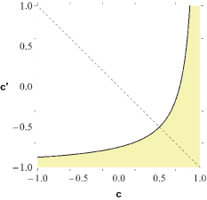
Figure 20: Assuming entanglement-breaking in each link ($n=2+10^{-4}\gtrsim 2$) and arbitrary entanglement at the input ($\mu>1$), we characterize the region of the classical correlation plane $(c,c^{\prime})$, depicted in yellow, where entanglement swapping is reactivated, i.e., the condition of Eq. (112) is satisfied.

In the correlation plane, we can identify an optimal point $(c,c^{\prime})=(1,-1)$. This extremal point describes an environment whose classical correlations are able to completely cancel the noise from the output modes. In fact, by replacing in $\mathbf{V}_{ab|\gamma}^{\text{add}}(\mu,n,c,c^{\prime})$ of Eq. (111), we retrieve

$$\mathbf{V}_{ab|\gamma}^{\text{add}}(\mu,n,1,-1)=\frac{1}{2\mu}\left(\begin{array}[c]{cc}(\mu^{2}+1)\mathbf{I}&(\mu^{2}-1)\mathbf{Z}\\ (\mu^{2}-1)\mathbf{Z}&(\mu^{2}+1)\mathbf{I}\end{array}\right),$$

which is the CM of a swapped state in absence of loss and noise (as one can also double-check by applying the formulas in Refs. GaussSWAP ). Such an environment has such a unique property since it corresponds to the quadrature transformations of Eq. (97) with $\xi_{2}=\xi_{1}$ and $\xi_{4}=-\xi_{3}$, so that, after the beam splitter of the relay, we have

$$\hat{q}_{-} =\frac{\hat{q}_{A^{\prime}}-\hat{q}_{B^{\prime}}}{\sqrt{2}}=\frac{\hat{q}_{A}-\hat{q}_{B}}{\sqrt{2}},$$

$$\hat{p}_{+} =\frac{\hat{p}_{A^{\prime}}+\hat{p}_{B^{\prime}}}{\sqrt{2}}=\frac{\hat{p}_{A}+\hat{p}_{B}}{\sqrt{2}}.$$

Thanks to the global cancelation effect induced by its correlations, the optimal environment $(1,-1)$ not only reactivates entanglement swapping but any other quantum protocol.

Besides the optimal point $(1,-1)$ and the Markovian point $(0,0)$ (which is unable to reactivate), there are infinite other points in the plane $(c,c^{\prime})$ with intermediate performances. An interesting environment corresponds to the sub-optimal point $(1,1)$ for which we have the following CM for the swapped state

$$\mathbf{V}_{ab|\gamma}^{\text{add}}(\mu,n,1,1) =\left(\begin{array}[c]{cc}\mu\mathbf{I}&\mathbf{0}\\ \mathbf{0}&\mu\mathbf{I}\end{array}\right)-\frac{\mu^{2}-1}{2}\times$$ (115)

$$\times\left(\begin{array}[c]{cccc}\frac{1}{\mu}&0&\frac{-1}{\mu}&0\\ 0&\frac{1}{\mu+2n}&0&\frac{1}{\mu+2n}\\ \frac{-1}{\mu}&0&\frac{1}{\mu}&0\\ 0&\frac{1}{\mu+2n}&0&\frac{1}{\mu+2n}\end{array}\right).$$ (120)

This environment cancels the noise in only one quadrature and corresponds to the transformations of Eq. (97) with $\xi_{2}=\xi_{1}$ and $\xi_{4}=\xi_{3}$, so that, after the beam splitter of the relay, we have

$$\hat{q}_{-}=\frac{\hat{q}_{A}-\hat{q}_{B}}{\sqrt{2}},~{}\hat{p}_{+}=\frac{\hat{p}_{A}+\hat{p}_{B}+2\xi_{3}}{\sqrt{2}}.$$

Despite the fact that this sub-optimal environment reactivates entanglement swapping, its effects on the other quantum protocols, in particular, the practical QKD protocol, need to be investigated (see below).

Sec. 3.3 Relay-based practical QKD

In order to study the reactivation properties of the correlated-additive environment, we consider the quantum protocol most difficult to reactivate, i.e., the practical QKD protocol (such property is inherited via the continuous limit from the previous correlated-thermal environment). The analysis of Sec. 2.8, based on the use of the entropic equalities $S(\rho_{\mathbf{E}|\gamma})=S(\rho_{ab|\gamma})$ and $S(\rho_{\mathbf{E}|\gamma\alpha})=S(\rho_{b|\gamma\alpha})$, is valid for any physical value of the parameters $\tau$, $\omega$, $g$ and $g^{\prime}$ of the correlated-thermal environment. Therefore, it continues to be valid in the considered limit for $\tau\rightarrow 1$ and $\omega\rightarrow+\infty$ with the constraints specified by Eq. (94).

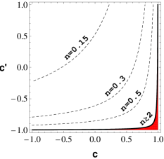
Figure 21: Security thresholds $R=0$ plotted on the correlation plane $(c,c^{\prime})$ for increasing values of the additive noise $n$ (signal modulation $\mu\simeq 52$ and reconciliation efficiency $\xi=1$). The solid curve is the security threshold for entanglement-breaking links ($n=2+10^{-4}\gtrsim 2$): The points in the red region are environments whose classical correlations are strong enough to reactivate the QKD protocol.

The net effect of this limit is the re-definition (100) of the $\kappa$-parameters in the secret-key rate $R(\xi,\mu,\kappa,\kappa^{\prime})$ of Eq. (86). Thus, the analytical expression of the key rate in the correlated-additive environment is given by

$$R_{\text{add}}(\xi,\mu,n,c,c^{\prime})=R[\xi,\mu,(1-c)n,(1+c^{\prime})n].$$

Let us fix a value for the reconciliation efficiency (e.g., $\xi=1$) and a finite value for the modulation variance (e.g., $\mu=52$). Then, for any value of the additive noise $n$, we can plot the security threshold $R_{\text{add}}=0$ on the classical correlation plane $(c,c^{\prime})$, as done in Fig. 21.

As we can see, a positive key rate can be extracted in the presence of entanglement-breaking channels as long as the classical correlations of the environment are sufficiently high (see the red ‘reactivating region’ in the figure). The best reactivating environment is clearly the extremal bottom-right point $(c,c^{\prime})=(1,-1)$. At some specified point, e.g., the suboptimal point $(1,1)$, we can plot the rate $R_{\text{add}}$ as a function of $n$. This is done in Fig. 22, where the rate is shown to be positive in the entanglement-breaking range $2<n\leq 4$. In the following experimental implementation, we show that this behavior is robust to the presence of loss.

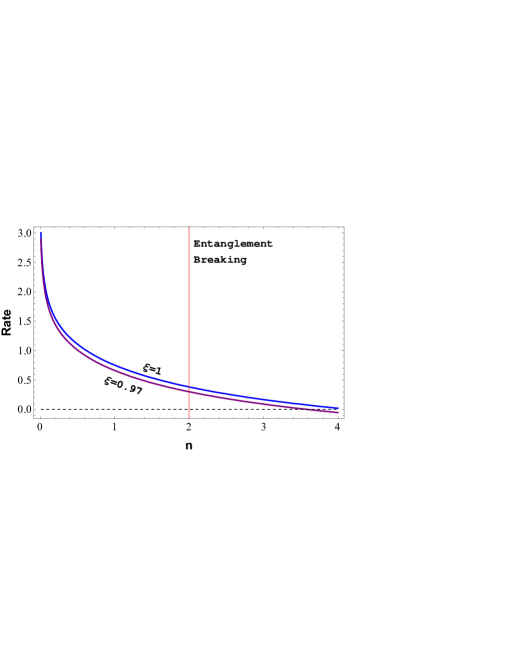
Figure 22: Rate $R_{\text{add}}(\xi,52,n,1,1)$ in bits/use as a function of the additive noise $n$, for $\xi=1$ and $\xi\simeq 0.97$.

Sec. 4 Experimental Methods

Sec. 4.1 Description of the setup

Our theoretical results are confirmed by the proof-of-principle experiment, whose setup is schematically depicted in Fig. 6 of the main text. Here Alice and Bob receive 1064 nm light from the same laser source (common local oscillator), divided amongst them by a balanced beamsplitter. At both stations, the incoming beams are Gaussianly modulated in phase and amplitude using independent electro-optical modulators driven by uncorrelated signal generators. Unwanted correlations between different quadratures are remedied by purifying the polarization of the light entering the modulators with a combination of waveplates and polarizing beamsplitters. In this way the two parties are able to generate random coherent states with independent Gaussian modulations in the two quadratures on top of the common local oscillator.

Simultaneously, the phase and amplitude modulators are subject to a side-channel attack Gisin ; mdiQKD : Additional electrical inputs are introduced by Eve, whose effect is to generate additional and unknown phase-space displacements. In particular, Eve’s electrical inputs are perfectly correlated so that the resulting optical displacements introduce a correlated-additive Gaussian environment with CM (98) $\mathbf{V}\left(n,c\simeq 1,c^{\prime}\simeq 1\right)$, i.e., the suboptimal point $(1,1)$ previously discussed. The magnitudes of the correlated noise modulations are incrementally increased from $n=0$ to $n=4$ ($\simeq 4.8$dB) via $0.2$dB-steps, and kept symmetric between the quadratures. Simultaneously, the signal modulations are kept constant at the same level in both quadratures for both Alice and Bob, realizing the constant modulation variance of $\mu\simeq 52$ shot noise units.

The optical modes then reach the midway Charlie, i.e., the relay. Here the two modes interfere at a balanced beam splitter with very high visibility ($>99\%$) and their relative phase is controlled by using a piezo mounted mirror in such a way to produce equally intense beams at the output. The output beams are then focused onto two balanced and highly-efficient photodetectors. Their photocurrents are subtracted and added to produce both the difference of the amplitude quadratures and the sum of the phase quadratures, respectively. The overall quantum efficiency of the relay is around $98\%$.

Even if small, the additional loss associated with the experimental imperfections must be ascribed to Eve. This means that, besides the side-channel attack of Alice’s and Bob’s private spaces, Eve is also assumed to actively attack the two external links with the relay. Globally, we then assume that Eve performs a coherent two-mode Gaussian attack affecting the modes both inside and outside the private spaces. As explained before, we can handle this worst-case scenario because we can derive the key rate directly from Alice and Bob’s shared data, assuming that Eve possesses the whole environmental purification compatible with this data (see Sec. 2.8.1). The presence of additional loss clearly worsens the performance of the protocol but also makes the implementation more interesting since it proves that the reactivation phenomenon may indeed occur in a realistic lossy environment.

In our experiment, it is worth noticing that the detection method is enabled by the brightness of the carrier and represents a simple alternative to the standard eight-port measurement setup which is typically needed for implementing the CV Bell detection UlrikPRL . Furthermore, as the subtraction/addition processes are performed in a software program, an imbalanced hardware-system can be compensated during the post-processing.

All measurements are done at a sideband frequency of $10.5$MHz. This is done in order to avoid the low frequency noise close to the carrier frequency and in turn provides a quantum noise limited signal. The power of the individual beams before the detectors was about $1.4$mW. The received signal is mixed down to dc from the measurement frequency of $10.5$MHz. The dc signal is low pass filtered at $100$kHz to set the detection bandwidth and is digitized with $500$kHz sampling rate and $14$bit resolution. Our data blocks are $10^{6}$ and thus long enough for our secret-key rate to converge to its asymptotic value, which is achieved after $10^{6}$ data points.

Sec. 4.2 Experimental secret key rate

Eve’s electric signals sent to the modulators have the effect to create random displacements on the optical modes, in such a way to generate an optical Gaussian environment with correlated-additive noise. Besides this, we also have loss at the untrusted relay which must be ascribed to Eve in the worst-case scenario. From the point of view of Alice and Bob, Eve’s actions are globally perceived as a coherent Gaussian attack of the two optical modes. All the environmental ancillas used by Eve are stored in a quantum memory, which is coherently detected at the end of the protocol.

As typical in QKD, Alice and Bob publicly disclose a subset of their data. Thus, they are able to reconstruct the joint Gaussian statistics of the three main variables of the protocol, i.e., their encodings and the outcome of the relay $\gamma$. From the second-order statistical moments they can compute the experimental CM $\mathbf{V}_{ab|\gamma}^{\text{exp}}$ associated with the entanglement-based representation of the protocol.

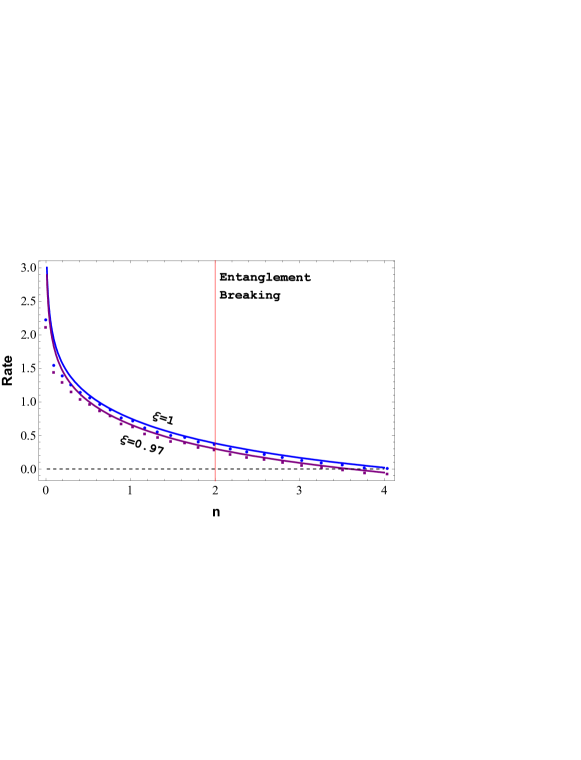
Figure 23: Experimental key rate (bits/use) assuming ideal reconciliation ($\xi=1$, blue circles) and realistic reconciliation efficiency ($\xi\simeq 0.97$, purple squares). Modulation variance is $\mu\simeq 52$. Due to loss, the experimental rates are slightly below the theoretical curves associated with the side-channel attack, corresponding to a correlated-additive environment with $(c,c^{\prime})=(1,1)$. Additive noise $n$ is increased beyond the entanglement-breaking threshold ($n>2$). We can see that the experimental key rate is positive in the region $2<n\leq 4$. The reactivation of QKD from entanglement-breaking is experimentally confirmed.

Once this CM is known, they can derive the experimental secret-key rate, following the steps of Sec. 2.8.1. From $\mathbf{V}_{ab|\gamma}^{\text{exp}}$ they can compute its symplectic spectrum and the matrices $\mathbf{V}_{b|\gamma}^{\text{exp}}$ and $\mathbf{V}_{b|\gamma\alpha}^{\text{exp}}$. Thus, they can compute the mutual information via Eq. (82) and Eve’s Holevo information via Eq. (84). By replacing these quantities in Eq. (85), they then derive the experimental value of the secret key rate $R_{\text{exp}}(\xi)$. This is the rate that Alice and Bob would achieve by post-processing their data via classical codes with reconciliation efficiency $\xi$.

As we can see from Fig. 23 (and the corresponding Fig. 5 in the main text), the experimental key rate is slightly below the theoretical prediction which is computed for the correlated-additive environment induced by the side-channel attack. This discrepancy comes from the presence of additional (small) loss at the relay station which clearly degrades the performance of the realistic protocol. From Fig. 23 we see that the experimental rate remains positive after the entanglement-breaking threshold. (Note that the entanglement-breaking condition $n>2$, derived for the additive-noise environment, continues to hold, approximately, when small loss is present.)

Sec. 5 Further Discussion

We clarify some points which may help the readers to better understand the impact of our results. In the first subsection we discuss a simple example of reactivation with qubits. This example is rather artificial and is only provided to clarify the conditions where the phenomenon of reactivation becomes non-trivial. In the second subsection we explain the relations with previous literature.

Sec. 5.1 Reactivation with discrete variables

Consider the protocol of entanglement swapping in a lossless environment known as $U\otimes U^{\ast}$-twirling. This is realized by a classical mixture of operators of the type $U\otimes U^{\ast}$, with $U$ being a unitary. Suppose that Alice and Bob possess two Bell pairs, $\rho_{aA}$ and $\rho_{bB}$, respectively. For instance, each pair may be a singlet state $\left(\left|0,1\right\rangle-\left|1,0\right\rangle\right)/\sqrt{2}$. Qubits $a$ and $b$ are retained, while traveling qubits $A$ and $B$ are subject to twirling, so that their reduced state $\rho_{AB}$ is transformed as

$$\rho_{A^{\prime}B^{\prime}}=\int dU~{}(U\otimes U^{\ast})~{}\rho_{AB}~{}(U\otimes U^{\ast})^{\dagger}~{},$$ (121)

where the integral is over the entire unitary group $\mathcal{U}(2)$ acting on the bi-dimensional Hilbert space and $dU$ is the Haar measure.

On the one hand, this environment is locally entanglement breaking. In fact, by taking the partial traces of Eq. (121), we can see that the two channels $\rho_{A}\rightarrow\rho_{A^{\prime}}$ and $\rho_{B}\rightarrow\rho_{B^{\prime}}$ are completely depolarizing. On the other, the application of a Bell detection on the output qubits $A^{\prime}$ and $B^{\prime}$ has the effect to completely cancel the environmental noise. In fact, one can easily check, the output state of the remote qubits $a$ and $b$ will be projected onto a singlet state up to a Pauli operator, which can be “undone” thanks to the communication of the Bell outcome.

This example is artificial because it heavily relies on the fact that environment is lossless (no qubit is lost) and the action of the unitaries is very specific, i.e., they are perfectly correlated and of the twirling type $U\otimes U^{\ast}$. In the presence of loss, this perfect noise-cancelation rapidly tends to disappear. This is why the study of the reactivation phenomenon becomes non-trivial in realistic lossy environments. From this point of view, it is known that the quantum systems which are more fragile to loss are CV systems, which is why the study of reactivation is absolutely non-trivial for bosonic modes in lossy Gaussian environments.

Sec. 5.2 Main results and relations with other literature

To our knowledge ours is the first work where:

1. The basic CV relay-based protocols of entanglement swapping, quantum teleportation, entanglement/key distillation are studied and extended to non-Markovian conditions.

2. Weak non-Markovian effects (modelled by separable correlations) are shown to reactivate these relay-based protocols back from standard (Markovian) conditions of entanglement breaking.

3. The survival of a multi-partite form of entanglement provides a physical resource which can be localized and then exploited by the previous protocols (directly or indirectly).

4. The reactivation of a quantum relay is experimentally demonstrated.

5. As explained in the main text, we experimentally show that the single-repeater bound RepBound can be overcome by the presence of classical (separable) correlations in the bosonic environment.

These main achievements have a limited overlap with previous results in the literature. Ref. NJPpirs is a theoretical-only study which considered a different configuration, that where Charlie (in the middle) has an entangled source to be distributed to Alice and Bob. Despite this configuration of direct entanglement distribution can be seen (by some authors) as a reverse formulation of entanglement swapping, the two schemes are inequivalent and very well distinguished by the community.

The distinction between direct entanglement distribution and entanglement swapping is really important and is at the basis of different branches of quantum information protocols. For instance, direct entanglement distribution plays an important role in device-independent QKD, testing of non-locality etc. By contrast, entanglement swapping is the core technique for quantum repeaters, MDI-QKD (i.e., semi device independent QKD), etc. It is clear that showing a new effect or property for one of the two configurations does not automatically extend to the other.

Let us further discuss the basic differences between direct entanglement distribution and entanglement swapping:

• In CVs, entanglement swapping is much more fragile than direct entanglement distribution. In fact the two protocols have well-known different performances in the presence of loss. For example, in the non-Markovian environment considered in our paper and considering the limit of large $\mu$, the remote entanglement distributed to Alice and Bob is quantified by smallest (and asymptotical) PTS eigenvalue

  $$\varepsilon_{\text{opt}}=(1-\tau)\sqrt{(\omega-g)(\omega+g^{\prime})},$$

  for the case of direct distribution, and by

  $$\varepsilon_{\text{opt}}=\frac{1-\tau}{\tau}\sqrt{(\omega-g)(\omega+g^{\prime})},$$

  for the case of entanglement swapping. The analytical simplification induced by the limit $\mu\rightarrow+\infty$ clearly shows the extra factor $\tau^{-1}$, which makes the performances of the two configurations completely inequivalent in the presence of loss.

• Entanglement swapping is conceptually more interesting for its connections with network implementations and the end-to-end principle. Contrarily to the case of direct entanglement distribution, where the central node (Charlie) must prepare quantum resources to be distributed, in the case of entanglement swapping Charlie needs only to perform a very cheap and efficient detection on the incoming systems. Removing quantum resources from intermediate nodes is a key step for the scalability of quantum protocols to large quantum networks.

• Specifically about the phenomenon of reactivation: this is possible in both configurations, but this is based on two inequivalent dynamics of the quantum correlations. In the direct distribution of entanglement, the injection of correlations from the environment can reactivate the transmission of bipartite entanglement from Charlie to Alice and Bob. In the entanglement swapping configuration, no bipartite entanglement (or even tripartite) can be transmitted even with the injection of separable correlations from the environment. The key resource is here quadripartite entanglement which is not directly exploitable by the parties but must be localized by the action of the relay. Thus the phenomenon relies on the survival of a multipartite form of quantum entanglement.

• Finally, we stress that the non-Markovian study of all the other relay-based protocols, i.e., quantum teleportation, quantum repeater (swapping plus distillation), key distillation and practical QKD, were not treated before (and no experimental implementation was done).

For completeness, we also discuss the relations between our work and previous literature on QKD, specifically Ref. Untrusted , where MDI-QKD with CV systems has been introduced. Together with Ref. Untrusted , the present work shares the basic structure of the QKD protocol and the necessity to perform a security analysis in the presence of environmental correlations. As discussed in Ref Untrusted , random permutations and quantum de Finetti arguments do not allow to reduce the most general coherent attack into simple one-mode Gaussian attacks of the links. In other words, the unconditional security must be tested against a two-mode Gaussian attack of the links which therefore involves the presence of correlations and non-Markovian effects.

Apart from this common ground, the novelties of the present work with respect to previous Ref. Untrusted are several and non-trivial. These include the following points:

• In the present work we study MDI-QKD in the presence of entanglement breaking. This is an extremely insecure scenario which has never been considered by previous literature.

• For the first time we show that non-Markovian effects (in the form of a suitable coherent Gaussian attack) may actually be beneficial for QKD. The fact that some coherent attacks may actually help the key distribution is an interesting new feature whose potentialities should further be explored.

• We experimentally realize the first two-mode side-channel attack of a CV QKD protocol.

References

- (1) Cover, T. M. & Thomas, J. A. Elements of Information Theory (2nd edition, John Wiley & Sons, Inc., Hoboken, New Jersey 2006).
- (2) Nielsen, M. A. & Chuang, I. L. Quantum Computation and Quantum Information (Cambridge University Press, Cambridge, 2000).
- (3) Bouwmeester, D. The Physics of Quantum Information: Quantum Cryptography, Quantum Teleportation, Quantum Computation (Springer-Verlag, Berlin, 2000).
- (4) Vedral, V. Introduction to Quantum Information Science (Oxford University Press, 2006).
- (5) Bengtsson I. & Życzkowski, K. Geometry of quantum states: An Introduction to Quantum Entanglement (Cambridge University Press, Cambridge 2006).
- (6) Barnett, S. Quantum Information (Oxford University Press, 2009)
- (7) Schumacher, B. & Westmoreland, M. Quantum Processes Systems, and Information (Cambridge University Press, Cambridge, 2010).
- (8) Holevo, A. Quantum Systems, Channels, Information: A Mathematical Introduction (De Gruyter, Berlin-Boston, 2012).
- (9) Watrous, J. The theory of quantum information (Cambridge University Press, Cambridge, 2018).
- (10) Weedbrook, C., Pirandola, S., Garcia-Patron, R., Cerf, N. J., Ralph, T. C., Shapiro, J. H. & Lloyd, S. Gaussian quantum information. Rev. Mod. Phys. 84, 621 (2012).
- (11) Braunstein, S. L. & van Loock, P. Quantum information with continuous variables. Rev. Mod. Phys. 77, 513 (2005).
- (12) Andersen, U. L., Neergaard-Nielsen, J. S., van Loock, P. & Furusawa, A. Hybrid quantum information processing. Nat. Phys. 11, 713–719 (2015)
- (13) Kurizki, G., Bertet, P., Kubo, Y., Mølmer, K., Petrosyan, D., Rabl, P., & Schmiedmayer, J. Quantum technologies with hybrid systems. Proc. Natl. Acad. Sci. USA 112, 3866-73 (2015).
- (14) Zukowski, M., Zeilinger, A., Horne, M. A. & Ekert, A. “Event ready detectors” Bell experiment via entanglement swapping. Phys. Rev. Lett. 71, 4287 (1993).
- (15) van Loock, P. & Braunstein, S. L. Unconditional teleportation of continuous-variable entanglement. Phys. Rev. A 61, 010302(R) (1999).
- (16) Polkinghorne, R.E.S. & Ralph, T. C. Continuous Variable Entanglement Swapping. Phys. Rev. Lett. 83, 2095 (1999).
- (17) Pirandola, S., Vitali, D., Tombesi, P. & Lloyd, S. Macroscopic Entanglement by Entanglement Swapping. Phys. Rev. Lett. 97, 150403 (2006).
- (18) Briegel, H.-J., Dür, W., Cirac, J. I. & Zoller, P. Quantum Repeaters: The Role of Imperfect Local Operations in Quantum Communication. Phys. Rev. Lett. 81, 5932 (1998)
- (19) Bennett, C. H. et al. Teleporting an unknown quantum state via dual classical and Einstein-Podolsky-Rosen channels. Phys. Rev. Lett. 70, 1895 (1993).
- (20) Furusawa, A., et al. Unconditional quantum teleportation. Science 282, 706 (1998).
- (21) Pirandola, S., Eisert, J., Weedbrook, C., Furusawa, A. & Braunstein, S. L. Advances in Quantum Teleportation. Nature Photon. 9, 641-652 (2015).
- (22) Braunstein, S. L. & Pirandola, S., Side-Channel-Free Quantum Key Distribution. Phys. Rev. Lett. 108, 130502 (2012).
- (23) Lo, H.-K., Curty, M. & Qi, B. Measurement-Device-Independent Quantum Key Distribution. Phys. Rev. Lett. 108, 130503 (2012).
- (24) Pirandola, S. et al. High-Rate Measurement-Device-Independent Quantum Cryptography. Nature Photon. 9, 397-402 (2015).
- (25) Lucamarini, M., Yuan, Z. L., Dynes, J. F. & Shields, A. J. Overcoming the rate-distance limit of quantum key distribution without quantum repeaters. Nature 557, 400 (2018).
- (26) Wang, X.-B., Yu, Z.-W. & Hu, X.-L. Twin-field quantum key distribution with large misalignment error. Phys. Rev. A 98, 062323 (2018).
- (27) Pirandola, S., Andersen, U. L., Banchi, L., Berta, M., Bunandar, D., Colbeck, R., Englund, D., Gehring, T., Lupo, C., Ottaviani, C., Pereira, J., Razavi, M., Shaari, J. S., Tomamichel, M., Usenko, V. C., Vallone, G., Villoresi, P. & Wallden, P. Advances in quantum cryptography. Preprint arXiv:1906.01645 (2019).
- (28) Metcalf, B. J., et al. Quantum teleportation on a photonic chip. Nature Photon. 8, 770–774 (2014).
- (29) Masada, G., et al. Continuous-variable entanglement on a chip. Nature Photon. 9, 316–319 (2015)
- (30) L. Steffen, L., et al. Deterministic quantum teleportation with feed-forward in a solid state system. Nature 500, 319 (2013).
- (31) Breuer, H.-P. & Petruccione, F. The Theory of Open Quantum Systems (Oxford University Press, Oxford, 2002).
- (32) Lassen, M., Berni, A., Madsen, L .S., Filip, R. & Andersen U. L. Gaussian Error Correction of Quantum States in a Correlated Noisy Channel. Phys. Rev. Lett. 111, 180502 (2013).
- (33) Tyler, G. A. & Boyd, R. W. Influence of atmospheric turbulence on the propagation of quantum states of light carrying orbital angular momentum. Opt. Lett. 34, 142 (2009).
- (34) Semenov, A. A. & Vogel, W. Quantum light in the turbulent atmosphere. Phys. Rev. A 80, 021802(R) (2009).
- (35) Boyd, R. W., Rodenburg, B., Mirhosseini, M. & Barnett, S. M. Influence of atmospheric turbulence on the propagation of quantum states of light using plane-wave encoding. Opt. Express 19, 18310 (2011).
- (36) Renner, R. Symmetry of large physical systems implies independence of subsystems. Nature Phys. 3, 645-649 (2007).
- (37) Renner, R. & Cirac, J. I. de Finetti representation theorem for infinite-dimensional quantum systems and applications to quantum cryptography. Phys. Rev. Lett. 102, 110504 (2009).
- (38) Horodecki, M., Shor, P. W. & Ruskai, M. B. General Entanglement Breaking Channels. Rev. Math. Phys. 15, 629 (2003).
- (39) Holevo, A. S. Entanglement-breaking channels in infinite dimensions. Problems of Information Transmission 44, 3 (2008).
- (40) Pirandola, S. End-to-end capacities of a quantum communication network. Commun. Phys. 2, 51 (2019). See also preprint arXiv:1601.00966 (2016).
- (41) Spedalieri, G., Ottaviani, C. & Pirandola, S. Covariance matrices under Bell-like detections. Open Syst. Inf. Dyn. 20, 1350011 (2013).
- (42) Pirandola, S., Serafini, A. & Lloyd, S. Correlation matrices of two-mode bosonic systems. Phys. Rev. A 79, 052327 (2009).
- (43) Pirandola, S. Entanglement reactivation in separable environments. New J. Phys. 15, 113046 (2013).
- (44) Giedke, G., Kraus, B., Lewenstein, M. & Cirac, J. I. Separability Properties of Three-mode Gaussian States. Phys. Rev. A 64, 052303 (2001).
- (45) Werner, R. F. & Wolf, M. M. Bound entangled Gaussian states. Phys. Rev. Lett. 86, 3658 (2001).
- (46) Vidal, G. & Werner, R. F. Computable measure of entanglement. Phys. Rev. A 65, 032314 (2002).
- (47) Eisert, J. Entanglement in quantum information theory. PhD thesis (Potsdam, February 2001).
- (48) Plenio, M. B. The logarithmic negativity: A full entanglement monotone that is not convex. Phys. Rev. Lett. 95, 090503 (2005).
- (49) Devetak, I. & Winter, A. Distillation of secret key and entanglement from quantum states. Proc. R. Soc. Lond. A 461, 207 (2005).
- (50) Schumacher, B. & Nielsen, M. A. Quantum data processing and error correction. Phys. Rev. A 54, 2629 (1996).
- (51) Lloyd, S. Capacity of the noisy quantum channel. Phys. Rev. A 55, 1613 (1997).
- (52) Pirandola, S., García-Patrón, R. Braunstein, S. L. & Lloyd, S. Direct and reverse secret-key capacities of a quantum channel. Phys. Rev. Lett. 102, 050503 (2009).
- (53) Eckstein, A., Christ, A., Mosley, P. J. & Silberhorn, C. Highly Efficient Single-Pass Source of Pulsed Single-Mode Twin Beams of Light. Phys. Rev. Lett. 106, 013603 (2011).
- (54) Eberle, T., Händchen, V. & Schnabel R. Stable control of 10 dB two-mode squeezed vacuum states of light. Opt. Express 21, 11546 (2013).
- (55) Pirandola, S., Laurenza, R., Ottaviani, C. & Banchi, L. Fundamental Limits of Repeaterless Quantum Communications. Nature Commun. 8, 15043 (2017).
- (56) J. Williamson, Am. J. Math. 58, 141 (1936).
- (57) A. Serafini, F. Illuminati, and S. De Siena, J. Phys. B 37, L21 (2004).
-
(58)
Let us consider an arbitrary two-mode Gaussian state
with the following mean value and CM
where , and are real blocks. Let heterodyne mode with complex outcome . The corresponding real outcome is achieved with probability
which is Gaussian with classical CM . Correspondingly, mode is projected on a conditional Gaussian state with mean value and CM. - (59) Pirandola, S., Spedalieri, G., Braunstein, S. L., Cerf, N. J. & Lloyd, S. Optimality of Gaussian Discord. Phys. Rev. Lett. 113, 140405 (2014).
- (60) K. Modi, A. Brodutch, H. Cable, T. Paterek, and V. Vedral, Rev. Mod. Phys. 84, 1655-1707 (2012).
- (61) P. Giorda and M. G. A. Paris, Phys. Rev. Lett. 105, 020503 (2010).
- (62) G. Adesso and A. Datta, Phys. Rev. Lett. 105, 030501 (2010).
- (63) Note that for a TMSV state with variance , the amount of two-mode squeezing in dB is given by the formula .
- (64) A quantum instrument is a quantum operation which can have both classical and quantum outputs. For each classical outcome, there is a corresponding completely positive map applied to the quantum systems Qinstrument . For instance, a quantum instrument may describe the global effect of a partial quantum measurement (i.e., applied on a subset of the initial systems). A quantum measurement applied to all quantum systems can be seen as quantum instrument with classical output only.
- (65) Devetak, I. &Winter, A. Relating Quantum Privacy and Quantum Coherence: An Operational Approach. Phys. Rev. Lett. 93, 080501 (2004).
- (66) Pirandola, S. Quantum discord as a resource for quantum cryptography. Sci. Rep. 4, 6956 (2014).
- (67) Jouguet, P., Kunz-Jacques, S., & Leverrier, A. Long-distance continuous-variable quantum key distribution with a Gaussian modulation. Phys. Rev. A 84, 062317 (2011).
- (68) Gisin, N., Ribordy, G., Tittel, W. & Zbinden, H. Quantum Cryptography. Rev. Mod. Phys. 74, 145 (2002).
- (69) Niset, J., Acín, A., Andersen, U. L., Cerf, N. J., García-Patrón, R., Navascués, M., & Sabuncu, M. Superiority of entangled measurements over all local strategies for the estimation of product coherent states. Phys. Rev. Lett. 98, 260404 (2007).