Flat band superconductivity in the square-octagon lattice

Abstract

The discovery of superconductivity in twisted bilayer graphene has triggered a resurgence of interest in flat-band superconductivity. Here, we investigate the square-octagon lattice, which also exhibits two perfectly flat bands when next-nearest neighbour hopping or an external magnetic field are added to the system. We calculate the superconducting phase diagram in the presence of on-site attractive interactions and find two superconducting domes, as observed in several types of unconventional superconductors. The critical temperature shows a linear dependence on the coupling constant, suggesting that superconductivity might reach high temperatures in the square-octagon lattice. Our model could be experimentally realized using photonic or ultracold atoms lattices.

I Introduction

It has been conjectured that the presence of flat bands in a two-dimensional system may give rise to room temperature superconductivity Volovik2018 . Indeed, while for a conventional BCS superconductor, the critical temperature scales exponentially with the inverse of the interaction strength, for a flat band system the critical temperature exhibits a linear dependence on the interaction Heikkla2011 ; Kopnin2011 , indicating a robust superconducting phase. The BCS result for narrow bands in the strong coupling limit becomes $T_{c}\propto gN(0)$ where $N(0)$ is the density of the states at the Fermi level, which is enhanced as the flat band leads to maximal values of the density of states Marchenko2018 .

The conjecture seems to be ratified by the discovery of superconductivity in twisted bilayer graphene Cao2018a : when two stacked sheets of graphene are twisted relative to each other by about 1.1 degrees, the so-called first “magic” angle, zero-resistance states with critical temperature of up to 1.7 K arise upon electrostatic doping. This emergent superconductivity is absent in a single layer graphene and occurs because the twisting leads to the formation of a Moiré pattern, and a consequent shift of the Van Hove singularity to the Fermi energy. This phenomenon has been predicted theoretically a few years ago Bistritzer2011 , but has been experimentally observed only recently Cao2018a ; Cao2018b . The general understanding is that due to the presence of flat bands, the kinetic energy is quenched and interaction-driven quantum phases prevail. A similar explanation has been proposed to interpret the appearance of high-$T_{c}$ superconductivity in highly oriented pyrolytic graphite Esquinazi2014 ; Kopelevich2015 .

The possibility to access flat bands and their influence on the physical properties of the system have been studied for about three decades Lieb1989 ; Mielke1991 ; Tasaki1992 ; Arita2002 ; Tanaka2003 ; Noda2009 ; Katsura2010 ; Julku2016 ; Hartman2016 ; Kumar2017 and recently there is a resurgence of interest in flat bands to explore unconventional superconductivity Peotta2015 ; Liang2017 ; Aoki2019 ; Kumar2019 ; Hoffmann2019 ; Sayyad2020 . In fact, given the implementation of experiments with cold atoms, photons or electrons in the micro and nanoscale respectively, many of the long-standing theoretical predictions for the flat band systems may finally be tested experimentally. Indeed, flat bands have been observed not only in electronic systems or spin chains with frustration Derzhko2015 ; Chalker2011 , but also in artificial lattices Leykam2018a , as in ultracold atomic gases Taie2015 ; Ozawa2017 ; Taie2018 ; An2018 or photonic devices Schulz2017 ; Maczewsky2017 ; Mukherjee2017 ; Real2017 ; Klembt2017 ; Whittaker2018 ; Leykam2018b .

Here we investigate the superconducting phase of the square-octagon lattice, which is the arrangement of the octagraphene Sheng2012 . The square-octagon lattice has been attracting much attention lately due to the plethora of novel phases predicted to occur in the system. They range from a quantum magnetic phase under the competition between temperature and on-site repulsive interaction Bao2014 , to topological insulating phases induced by spin-orbit coupling or non-Abelian gauge fields Yang2019 ; Yang2018 ; Kargarian2010 , and even high-temperature superconductivity with singlet s_±-wave paring symmetry Kang2019 . Moreover, it has been shown that trivial and nontrivial flat bands can be tuned on the square octagon lattice by considering the addition of next-nearest neighbour hopping and an external magnetic flux Biplab2018 ; Sil2019 .

In this paper, we calculate the superconducting phase due to on-site attractive interactions when the system presents perfectly flat bands. We obtain multiple superconducting domes, as observed in several strongly correlated compounds Das2016 and twisted graphene bilayer MacDonald2019 . Since we analyse the conditions for the appearance of superconductivity in the system, our conclusions may shed some light in the understanding of the experimental data for those unconventional superconductors as well.

This paper is structured as follows: in Sec. II we analyse the conditions for the appearance of flat bands in the square-octagon lattice assuming nearest neighbour (NN) and next-nearest neighbour (NNN) hoppings and the presence of an external magnetic flux. Then, in Sec. III we calculate the superconducting phase diagram. Our conclusions are presented in Sec. IV.

II Flat bands

The tight-binding model that describes the kinetic energy of spin 1/2 fermions in the square-octagon lattice (see Fig. 1) can be written as Sil2019 ,

$$H_{0}=\sum_{m,n}\sum_{i,j}\tau_{i,j}c^{\dagger}_{m,n,i,\sigma}c_{m,n,j,\sigma}+\mbox{ h.c.}\,,$$ (1)

where the operator $c^{\dagger}_{m,n,i,\sigma}$ ($c_{m,n,i,\sigma}$) creates (annihilates) a fermion with spin $\sigma=\uparrow,\downarrow$ at the $i$-th site of the $(m,n)$-th unit cell. $\tau_{i,j}$ is the hopping parameter between the $i$-th site and the $j$-th sites, and it can take two possible values, depending on the position of the sites $i$ and $j$. For an electron hopping along the boundary of a square plaquette, $\tau_{i,j}=t$, which is the NN hopping. Along the lines inside the square plaquettes, $\tau_{i,j}=\tau$, which denotes the NNN hopping. As shown in Fig. 1, the NN vectors are defined as ${\bf\delta}_{1}=\left(1/\sqrt{2}\right)(1,-1)$, ${\bf\delta}_{2}=\left(1/\sqrt{2}\right)(1,1)$, ${\bf\delta}_{3}=(0,1)$, and ${\bf\delta}_{4}=(1,0)$, while the NNN vectors are ${\bf\delta}_{5}=\sqrt{2}(0,1)$, and ${\bf\delta}_{6}=\sqrt{2}(1,0)$. The lattice parameter is set to unit for the sake of simplicity. The lattice translation vectors are ${\bf a}_{1}=(1+\sqrt{2},0)$ and ${\bf a}_{2}=(0,1+\sqrt{2})$, so that each unit cell is given by ${\bf R}(m,n)=m{\bf a}_{1}+n{\bf a}_{2}$ .

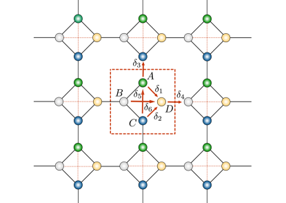
Figure 1: (Color online) The geometry of square-octagon lattice. $A,B,C,D$ denote four different sites in the unit cell, which indicate a large square (red dashed lines). The strength of the NN hopping along the sides (black solid lines) of the small square is $t$. The strength of the NNN hopping (red dotted lines) along the diagonals of the small square is $\tau$. $\delta_{1},\delta_{2},\delta_{3},\delta_{4}$ are NN vectors and $\delta_{5},\delta_{6}$ are NNN vectors.

Now, we assume that for each square plaquette there are Aharonov-Bohn phase factors incorporated to the hopping terms, $t\rightarrow t\,\exp(\,\pm i\Theta\,)$, due to the presence of an external magnetic flux $\Phi$ (or some artificial gauge field). Here, $\Theta=\pi\,\Phi/2\Phi_{0}$, with $\Phi_{0}=hc/e$ denoting the fundamental flux quantum. The positive and negative signs in the exponent indicate the direction of the forward and backward hoppings, respectively. By performing a Fourier transformation and introducing the spinor $\psi_{{\bf k},\sigma}=(c^{A}_{{\bf k},\sigma},c^{B}_{{\bf k},\sigma},c^{C}_{{\bf k},\sigma},c^{D}_{{\bf k},\sigma})^{T}$, where $c^{\alpha}_{{\bf k},\sigma}$ are the fermion annihilation operators in the four basis of the unit cell ($\alpha=A,B,C,D$, as in Fig. 1), with $k_{1}={\bf k}\cdot{\bf a}_{1}$ and $k_{2}={\bf k}\cdot{\bf a}_{2}$, the Hamiltonian in Eq. (1) becomes $H=-\sum_{{\bf k},\sigma}\psi^{\dagger}_{{\bf k},\sigma}\,\tilde{H}_{0}\,\psi_{{\bf k},\sigma}$, where Biplab2018

$$\tilde{H}_{0}=\left(\begin{array}[]{cccc}0&te^{i\Theta}&te^{ik_{2}}+\tau&te^{-i\Theta}\\ te^{-i\Theta}&0&te^{i\Theta}&te^{-ik_{1}}+\tau\\ te^{-ik_{2}}+\tau&te^{-i\Theta}&0&te^{i\Theta}\\ te^{i\Theta}&te^{ik_{1}}+\tau&te^{-i\Theta}&0\\ \end{array}\right)\,.$$ (6)

From now on, we set $t=1$ throughout this work without any loss of generality, and $\tau$ is given in units of $t$.

The particular case $\Theta=\tau=0$, i.e., when there is no magnetic flux and NNN hopping is neglected, has been previously investigated by Yamashita et al.Yamashita2013 . It was shown that the system is metallic and there are Dirac cones in the first Brillouin zone, with flat bands only along the lines $k_{1}=\pi$ or $k_{2}=\pi$.

The band solutions $\epsilon$ for the generic case of finite $\tau$ and $\Theta\neq 0$ can be quite complicated, since they are provided by the solutions of the equation

$$|\,\tilde{H}_{0}-\epsilon{\bf 1}\,|=F+G=0$$ (7)

for each spin channel, where

$$F = \epsilon^{4}-2\epsilon^{2}\left[\,\tau^{2}+\tau\,f(k_{1},k_{2})+3\,\right]$$ (8)

$$-4\epsilon\cos 2\Theta\left[\,f(k_{1},k_{2})+2\tau\,\right]\,,$$

$$G = \tau^{4}+2\tau^{3}f(k_{1},k_{2})+2\tau^{2}\left(\,2\cos k_{1}\cos k_{2}-1\,\right)$$ (9)

$$-2\tau f(k_{1},k_{2})-2\cos 4\Theta+3$$

$$-4\cos k_{1}\cos k_{2}\,,$$

and $f(k_{1},k_{2})=\cos k_{1}+\cos k_{2}$.

However, a simple possible condition for the appearance of flat bands in the model is obtained for $G=0$. In this case, one can see from Eq. (8) that there is at least one flat band, at $\epsilon=0$. Let us consider for the moment $\Theta=0$. Under this constraint, there are four values for the hopping $\tau$ satisfying $G=0$: $\tau=\pm 1,\tau_{\pm}$, where

$$\tau_{\pm}=f(k_{1},k_{2})\pm\sqrt{\frac{f(2k_{1},2k_{2})-4(\cos k_{1}\cos k_{2}-1)}{2}}\,.$$ (10)

The roots $\tau_{\pm}$ indeed correspond to a flat band $\epsilon=0$, but since the solutions are functions of $k_{1}$ and $k_{2}$, the adjustable parameter $\tau=\tau_{\pm}$ cannot be easily used in experiments in order to engineer a model with flat bands. In contrast, for $\tau=\pm 1$, we obtain not just one, but rather two flat band solutions from Eq. (9): For $\tau=-1$, there are flat bands at

$$\epsilon_{1,2}=2,0\,,$$ (11)

and dispersive bands at

$$\epsilon_{3,4}=-1\pm\sqrt{5-2f(k_{1},k_{2})}\,,$$ (12)

whereas for $\tau=1$ the bands are

$$\epsilon=\begin{cases}\,0\,,\\ \,-2\,,\\ \,1\pm\sqrt{5+2f(k_{1},k_{2})}.\end{cases}$$ (13)

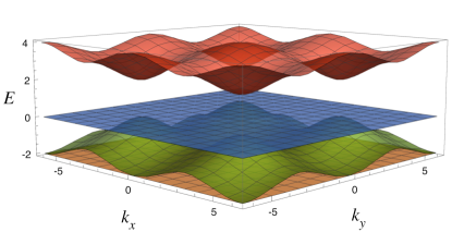
Figure 2: (Color online) Band structure of the noninteracting tight-binding square-octagon lattice model in momentum space. $\tau=1$, $\Theta=0$, and the energies are expressed in units of $t$.

The band structure for $\tau=1$ and $\Theta=0$ has been previously investigated Biplab2018 ; Sil2019 and a remarkable feature for the square-octagon lattice is that one of the dispersive bands is sandwiched in between two perfectly flat bands, while the other is isolated from the rest, at the top of the spectrum, as depicted in Fig. 2.

As emphasized in Ref. Biplab2018 , this is a remarkable result, very different from the usual flat bands that appear only at the maximum or minimum of the spectrum in absence of any magnetic field Ohgushi2000 ; Bergman2008 .

Notice that, within the first Brillouin zone, the sandwiched dispersive band touches the higher flat band ($\epsilon=0$) at ${\bf k}=(\pm\pi,\pm\pi)$ and the lowest flat band at ${\bf k}=(0,0)$.

Moreover, numerical calculations Biplab2018 indicate that flat bands appear even in the presence of a magnetic flux and remain robust for fairly high values of the flux, although they are not observed for every non-zero value of $\Theta$. Indeed, our studies ratify the numerical results, since it can be promptly verified analytically from Eq. (7) that perfectly flat bands arise for $\tau=1$ and $\Theta\neq 0$,

$$|\,\tilde{H}_{0}-\epsilon{\bf 1}\,|=F-2\left(\,\cos 4\Theta-1\,\right)=0\,.$$ (14)

Thus, whenever $\cos 4\Theta=1$, one obtains at least one flat bland, $\epsilon=0$, and hence $\Theta=n\,\pi/2$, with $n\in\mathbb{Z}$. In particular, for this specific choice of $\Theta$ and $\tau=1$, we get two flat bands and also two other dispersive bands,

$$\epsilon=\begin{cases}\,0\,,\\ \,2l\,,\\ \,-l\pm\sqrt{5+2f(k_{1},k_{2})}\,,\end{cases}$$ (15)

where $l=\pm 1$ for odd or even values of $n$, respectively. Therefore, from now on, we set $\tau=1$ and $\Theta=n\pi/2$ for even values of $n$ in the remaining of this paper.

Although we have concentrated here on the case $\tau=1$ and $n$ even for the magnetic flux quantization, $\Theta=n\pi/2$, the results for $n$ odd or $\tau=-1$ are essentially the same, since one still obtains two perfectly flat bands and two dispersive bands, where one of the bands is detached from the others and the remaining is sandwiched between the two flat bands.

Finally, the Chern numbers have been calculated for each of the bands Biplab2018 with $\Phi\neq 0$ and, as expected, the dispersive bands are trivial, but nearly flat bands present nonzero Chern numbers.

III On-site pairing interactions

Let us now turn our attention to the effect of interactions in the system by introducing an on-site Hubbard-like attractive term, expressed as $-g\,n^{\alpha}_{\uparrow}n^{\alpha}_{\downarrow}$, where $g>0$ is the interaction strength and $n^{\alpha}_{\sigma}$ is the number operator for fermions, with $\alpha=A,B,C,D$ labelling the basis of the unit cell, as before. Taking into account every site of the lattice, the interaction Hamiltonian can be rewritten as

$$H^{\mbox{\scriptsize{on-site}}}_{int}=-g\sum_{\alpha,i}\left(p^{\alpha}_{i}\right)^{\dagger}p^{\alpha}_{i}\,,$$ (16)

where the operator $p^{\alpha}_{i}=c^{\alpha}_{i,\downarrow}c^{\alpha}_{i,\uparrow}$ destroys a Cooper pair at the $i$-th site of the lattice and its adjoint $\left(p^{\alpha}_{i}\right)^{\dagger}$ creates a Cooper pair.

In a flat band, the interactions dominate over the kinetic energy, which suggests that a mean-field calculation might be appropriate to describe the superconducting phase. Therefore, the Fourier transform of Eq. (16) becomes

$$\tilde{H}^{\mbox{\scriptsize{on-site}}}_{int}=-\sum_{\alpha,\bf k}\left[\,\left(p^{\alpha}_{\bf k}\right)^{\dagger}\Delta+p^{\alpha}_{\bf k}\Delta^{*}-\frac{|\Delta|^{2}}{g}\,\right]\,,$$ (17)

where we have introduced the superconducting order parameter, $\Delta=-g\sum_{\bf k}c^{\alpha}_{-\bf k,\downarrow}c^{\alpha}_{\bf k,\uparrow}$ and we have also assumed that $\Delta^{\alpha}\equiv\Delta$.

Now, taking the spinor $\psi_{\bf k,\sigma}$ introduced above and defining the Nambu operator $\Psi^{\dagger}_{\bf k}=\left(\,\psi^{\dagger}_{\bf k,\uparrow};\,\psi^{T}_{\bf k,\downarrow}\,\right)$, one can combine the noninteracting Hamiltonian in Eq. (6) with the interaction term in Eq. (17), so that our model Hamiltonian becomes $H=\sum_{{\bf k}}\Psi^{\dagger}_{{\bf k}}\,\tilde{H}\,\Psi_{{\bf k}}$, where

$$\tilde{H} = \left(\begin{array}[]{cc}\tilde{H}_{0}-\mu&H_{\Delta}\\ H_{\Delta^{*}}&-\tilde{H}_{0}+\mu\end{array}\right)\,,$$ (20)

and we have introduced the chemical potential $\mu$, with $H_{\Delta}=\Delta\times{\bf 1}_{4}$, where ${\bf 1}_{4}$ is the 4 $\times$ 4 identity matrix. Therefore, the eigenvalues of our model Hamiltonian are

$$E= \pm\sqrt{\,\mu^{2}+|\Delta|^{2}\,}\,,$$ (21a)

$$E= \pm\sqrt{\left(2+\mu\right)^{2}+|\Delta|^{2}}\,,$$ (21b)

$$E= \pm\sqrt{\left(\,|1-\mu|-\xi\,\right)^{2}+|\Delta|^{2}}\,,$$ (21c)

$$E= \pm\sqrt{\left(\,|1-\mu|+\xi\,\right)^{2}+|\Delta|^{2}}\,,$$ (21d)

where $\xi=\sqrt{5+2f(k_{1},k_{2})}$. Notice that for $\Delta=\mu=0$ we get $E=\pm|\epsilon|$, where $\epsilon$ are the energies of the noninteracting system, with $l=-1$ in Eq.(15). In addition, Eqs. (21a) and (21b) is related to the flat bands obtained previously, while Eqs. (21c) and (21d) to the remaining dispersive bands. Since the band given by Eq. (21d) is detached from the others, we will consider an effective model from now on that disregards it.

The condition for the appearance of superconductivity is provided by the nonzero values of $\Delta$ that minimize the free energy (effective potential), given by

$$V_{\rm{eff}}=\frac{|\Delta|^{2}}{g}-T\sum_{n}\,\int\frac{d^{2}k}{\mathcal{A}}\,\log\left[\,\prod_{j=1}^{8}\left(i\omega_{n}-E_{j}\right)\,\right]\,,$$ (22)

where $T$ is the temperature, $\mathcal{A}$ is the area in momentum space, $\omega_{n}$ are the well known fermionic Matsubara frequencies and $j$ is the index for the eigenvalues in Eq. (21d). We have set $k_{B}=\hbar=1$ for the sake of simplicity.

Deriving $V_{\rm{eff}}$ with respect to $\Delta$, and performing the sum over $\omega_{n}$, we arrive at the gap equation,

$$1=\frac{g}{2}\sum_{j{\text{ (odd ) }}}\int\frac{d^{2}k}{\mathcal{A}}\,\frac{1}{E_{j}}\tanh\left(\frac{E_{j}}{2T}\right)\,,$$ (23)

where $j{\text{ (odd ) }}$ indicates that we are summing only over the first three positive values of $E$ in Eqs. (21a)-(21c).

From Eq. (23), we obtain the self-consistent equation for the critical temperature $T_{c}$, which is defined as the temperature at which $\Delta=0$,

$$\frac{1}{\Delta_{00}}=\frac{1}{|\mu|}\tanh\left(\frac{|\mu|}{2T_{c}}\right)+\frac{1}{|2+\mu|}\tanh\left(\frac{|2+\mu|}{2T_{c}}\right)+I\left(k_{c}\right)\,,$$ (24)

where

$$\Delta_{00}\equiv\frac{g}{2}\left[\,\frac{\mathcal{A}(k_{c})}{\mathcal{A}}\,\right]=\frac{g}{2}\left[\,\frac{1}{\mathcal{A}}\int_{|k|<k_{c}}d^{2}k\,\right]\,,$$ (25)

and

$$I\left(k_{c}\right)=\frac{1}{\mathcal{A}(k_{c})}\int_{|k|<k_{c}}d^{2}k\,\frac{1}{|\xi_{\mu}|}\tanh\left(\frac{|\xi_{\mu}|}{2T_{c}}\right)\,,$$ (26)

with $\xi_{\mu}=\xi-|1-\mu|$, and we have introduced the momentum cutoff $k_{c}$.

In order to calculate $T_{c}$ from Eq. (24), three parameters have to be given: $\Delta_{00}$, $\mu$ and $k_{c}$. Notice that a natural cutoff emerges from the theory, depending on the microscopic mechanism that is responsible for the Cooper pair formation. In the BCS theory, a natural cutoff is the Debye frequency, since the pairing is due to the electron-phonon interaction. Similarly, for the square-octagon lattice, a natural cutoff is given in terms of the inverse of the lattice constant, and we integrate the momentum over the first Brillouin zone. In such case, $\Delta_{00}=g/2$. Let us now expand $\xi$ in polar coordinates for small values of $k$, $\xi\sim\sqrt{9-k^{2}}$. Introducing the change of variables $x=(k/k_{c})^{2}$, we get $\xi(x)\sim 3\sqrt{1-\delta_{c}x}$, where the new parameter $\delta_{c}=(k_{c}/3)^{2}$ incorporates the momentum cutoff $k_{c}$. From that, one can rewrite Eq. (26) as

$$I(\mu,T_{c})=\int_{0}^{1}dx\,\frac{1}{|\,\xi_{\mu}(x)\,|}\tanh\left(\frac{|\,\xi_{\mu}(x)\,|}{2T_{c}}\right)\,.$$ (27)

From now on, we set $\delta_{c}=1$, which is equivalent to integrate over the first Brillouin zone.

III.1 Square-octagon lattice

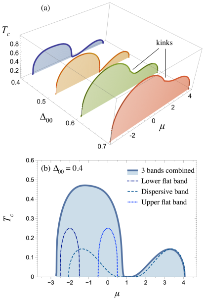
Figure 3: (Color online) a) Superconducting critical temperature $T_{c}$ as a function of the chemical potential $\mu$ for several values of $\Delta_{00}$. b) $T_{c}$ calculated individually for each band contribution compared with the combined results for $\Delta_{00}=0.4$. Energies are expressed in units of $t$.

The numerical results of $T_{c}$ as a function of $\mu$ for several values of $\Delta_{00}$ are presented in Fig. 3.

A unique feature for the square-octagon lattice is the kink at $\mu=1$, as indicated in Fig. 3(a) for $\Delta_{00}=0.6$ and $0.7$. This is due to the contribution of the dispersive energy in Eq. (21c), where a kink appears for the hyperbolic tangent at $\xi_{\mu}=0$ in Eq. (27), inducing a kink at $\mu=1$ in the phase diagram. As $\Delta_{00}$ decreases, a reentrant superconducting phase with two domes arises for $\Delta_{00}=0.4$ and $0.5$.

Interestingly, two-dome superconducting phase diagrams have been observed in several unconventional superconductors, as in cuprates, heavy-fermions, pnictides, chalcogenides and others Das2016 . Different theories have been proposed to explain the suppression of the superconductivity between the domes in those compounds. For the particular case of La-based cuprates, superconductivity is suppressed at $x\sim 0.125$ Buchner1994 , hence being called the 1/8 anomaly, and there is some consensus that this is due to the static stabilisation of stripes Tranquada1995 . For the Ce-based heavy fermion compounds, on the other hand, it has been suggested that the domes are related to different pairing mechanisms Yuan2014 , although a conclusion has not been reached yet Zeng2016 . For the YBCO compound, moreover, a richer scenario emerges as an external magnetic field is applied. In the absence of an external field, the domes are merged, which is similar to the data for the heavy-fermion CeCu₂Si₂ and also to our results in Fig. 3(a) for $\Delta_{00}=0.6$ and $0.7$. As an external magnetic field is applied, there are two superconducting domes, which closely resembles the data for La_2-x Ba_xCuO₄, at $x\sim 1/8$ and our results in Fig. 3(a) for $\Delta_{00}=0.4$ and $0.5$. For 50 T, only the second dome survives. Two possible scenarios have been proposed to explain the experimental data for YBCO Ranshaw2015 : independent pairing mechanisms, each responsible for a superconducting dome, as for the case of the Ce-based heavy fermion compounds; or a single pairing mechanism, where $T_{c}$ is reduced in the region between the domes. Presently, we argue that the two-dome phase diagram observed in unconventional superconductors can be related to a single pairing mechanism, specially when it is taken into account the multi-band aspect of the microscopic models that describe them.

Indeed, the emergence of these two superconducting domes in the square-octagon lattice is understood upon inspecting Fig. 3(b), where $T_{c}$ is calculated individually for each band in Eq. (23) for the particular case of $\Delta_{00}=0.4$. (The numerical results for different values of $\Delta_{00}$ in this range are qualitatively the same.) Notice that the first dome is essentially the combination of the three contributions in Eqs. (21a)-(21c), which are summed in a nonlinear way, as in Eq. (24), while the second dome is mainly provided by the dispersive band in Eq. (21c). We see that a single underlying pairing mechanism is responsible for the appearance of the two disconnected superconducting domes in the square-octagon lattice. Hence, we argue that the two-dome phase diagram observed in some unconventional superconductors can be related to a single pairing mechanism as well, specially when the multi-band aspect of the microscopic models that describe them is taken into account.

Another remarkable feature can be observed in Fig. 3(b) when we consider only the contribution of the flat bands for $\mu<1$. In this case, two superconducting domes are separated by an insulating phase, since the contribution from the dispersive band is disregarded. This resembles the phase diagram experimentally observed in twisted bilayer graphene MacDonald2019 . However, upon the contribution from the dispersive band sandwiched between the two flat bands, the superconducting domes become intertwined in the square-octagon lattice.

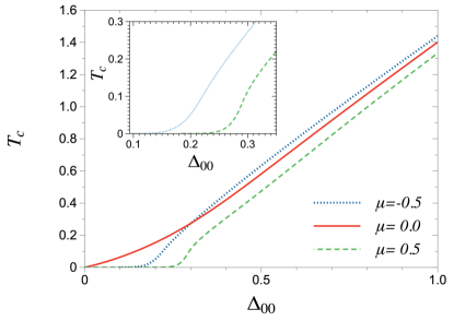
Figure 4: (Color online) Superconducting critical temperature $T_{c}$ as a function of the interaction strength $\propto\Delta_{00}$. Energies are expressed in units of $t$.

Next, we concentrate on the critical temperature $T_{c}$. The numerical results for $T_{c}$ as a function of $\Delta_{00}$ for several values of $\mu$ are presented in Fig. 4.

There seems to be an apparent threshold in the interaction strength for the appearance of superconductivity at finite values of the chemical potential. Per se, this defines a quantum critical point (QCP). However, the apparent suppression of the critical temperature for small values of $\Delta_{00}$ for $\mu=-0.5$ and $0.5$ is simply a steep exponential decay, as observed in the inset. Indeed, the absence of a QCP at $\mu=0$ in the square-octagon lattice can be demonstrated as follows: since the right-hand-side of Eq. (24) is a positive, unbounded and monotonically decreasing function of $T_{c}$ at $\mu=0$, given any positive value for $\Delta_{00}$, there is always a unique value for $T_{c}$ that satisfies the self-consistent equation, and, therefore there is no QCP at $\mu=0$. Moreover, while the contributions related to the flat bands are indeed bounded for finite values of the chemical potential, the contribution from the dispersive band $I(\mu,T_{c})$ diverges as $T_{c}\rightarrow 0$ (as demonstrated in the appendix) and, hence, there is no QCP for the square-octagon lattice even at $\mu\neq 0$.

Furthermore, for larger values of $\Delta_{00}$, there is a linear dependence of $T_{c}$ on $\Delta_{00}$. Since $\Delta_{00}\propto g$, the critical temperature scales linearly with the interaction strength. Such linear dependence was also obtained for generic flat-band superconductivity Heikkla2011 ; Kopnin2011 and should be contrasted with the exponential dependence of $T_{c}$ in conventional BCS superconductors, $T_{c}\sim\exp\left[-1/N(0)g\right]$, where $N(0)$ is the density of the states at the Fermi level. From there on, it has been conjectured that the superconducting critical temperature might reach room-temperatures for a system presenting flat bands Volovik2018 . Our results thus suggest that high-$T_{c}$ should be obtained in the square-octagon lattice, specially in the vicinity of $\mu=0$.

III.2 Generic flat band system

A superconducting QCP can be derived for a generic flat band system as follows: considering only the flat band $\epsilon=0$ in the Eq. (24), the critical temperature satisfies

$$\tilde{T_{c}}=\frac{|\tilde{\mu}|}{2\tanh^{-1}|\tilde{\mu}|}\,,$$ (28)

where we have defined $\tilde{T_{c}}=T_{c}/\Delta_{00}$ and $|\tilde{\mu}|=|\mu|/\Delta_{00}$. The real values for $T_{c}$ are constrained to $|\tilde{\mu}|<1$, which is equivalent to

$$g>2|\mu|\,,$$ (29)

assuming that $\Delta_{00}=g/2$ from the Eq. (25). The above equation defines a QCP whenever $\mu\neq 0$ and to the best of our knowledge, this is the first time that a QCP was derived for flat-band superconductivity. This is in contrast with 2D Dirac fermion systems, where there is a QCP at $\mu=0$ and the threshold is absent for $\mu\neq 0$ Marino2017 . It is curious that precisely the opposite applies for the flat-band superconductivity.

Moreover, assuming that the only relevant contribution in the self-consistent equation for $T_{c}$ arises from the flat band in Eq. (21a), and taking $\mu=0$, we get that $\Delta_{00}$ satisfies the gap equation and $\Delta_{00}/T_{c}=2$, which was obtained previously for flat-band superconductivity Heikkla2011 ; Kopnin2011 . This ratio is comparable to the results obtained experimentally for several high-$T_{c}$ superconductors Dagotto1994 .

IV Conclusions

In conclusion, in this paper we investigated the conditions for the appearance of flat bands in the square-octagon lattice. We found two perfectly flat bands with a dispersive band between them for equal values of NN and NNN hopping combined to an external magnetic flux, quantized as $\Theta=n\pi/2$, for even values of $n$.

Then, we introduced an on-site attractive interaction responsible for Cooper pairing and calculated the critical temperature for the two-dimensional system.

The superconducting phase diagram resembles those measured for unconventional superconductors Das2016 . In the square-octagon lattice, the disconnected superconducting domes are provided by the same underlying pairing mechanism and are related to the multi-band aspect of the system. We argue that the two-dome phase diagram observed in unconventional superconductors can be related to a single pairing mechanism as well.

Despite the steep reduction of $T_{c}$ for small values of the superconducting interaction strength, there is no QCP for the square-octagon lattice, but an exponential decay of $T_{c}$ for $\mu\neq 0$, given the presence of a dispersive band between the two flat bands. In contrast, we have derived the QCP for flat-band superconductivity, which occurs whenever $\mu\neq 0$. To the best of our knowledge, this is the first time that such a QCP was derived.

The linear dependence of the critical temperature on the coupling, as previously obtained for flat-band superconductivity Heikkla2011 ; Kopnin2011 , suggests that $T_{c}$ might reach very high temperatures in the square-octagon lattice.

The system discussed here could be experimentally realised using ultracold quantum gases in optical lattices. Interactions can be easily implemented using Feshbach resonances, but it might be challenging to design a laser setup that yields a square octagon lattice, and even more difficult, NN and NNN hopping of equal intensity. This problem can be easily solved by using electronic quantum simulators Slot2019 . In this case, lattices of any geometry can be promptly realised on the nanoscale, and the values of NN and NNN hopping can be controlled independently, with extreme precision. This occurs because the overlap integrals are designed by adjusting potential barriers, instead of the distance between lattice sites. Nevertheless, the currently investigated electronic quantum simulators rely on patterning adatoms on the surface state of copper, which is a non-interacting 2d electron gas, and interactions are not yet tunable. Further progress in the development of this platform is required to observe the phenomenon discussed here in designed structures.

Although we have focused the discussion of superconductivity on the square-octagon lattice, some results are generic, and valid for any system displaying flat bands. Indeed, we generalised the calculations in several instances to models with a generic flat band, and found that our results confirm previously obtained ones in some limits, and expands them. In particular, we find a striking similarity with the phase diagram observed experimentally in unconventional superconductors. Our studies might then shed further light on our understanding of these complex materials.

Appendix A Absence of a QCP

Here, we demonstrate that the contribution from the dispersive band is divergent when $T_{c}\rightarrow 0$ and therefore there is no QCP for the square-octagon lattice. Indeed, the integral in Eq. (27) can be broken in two parts, given the definition of the modulus. Employing the changes of variables,

$$y_{1,2}=\pm\left(\frac{a_{\mu}-3\sqrt{1-x}}{2T_{c}}\right)\,,$$ (30)

where $a_{\mu}=\left|1-\mu\right|$, Eq. (27) can be rewritten as

$$I(\mu,T_{c}) = \frac{2}{9}\left[\int_{0}^{a_{\mu}/2T_{c}}dy_{1}\left(\,\frac{a_{\mu}}{y_{1}}-2T_{c}\,\right)\tanh y_{1}\right.$$ (31)

$$+\left.\int_{0}^{\left(3-a_{\mu}\right)/2T_{c}}dy_{2}\left(\,\frac{a_{\mu}}{y_{2}}+2T_{c}\,\right)\tanh y_{2}\right]\,.$$

The r.h.s. in the above expression contains four terms, the second and the fourth terms are proportional to $T_{c}$ and bounded in the limit $T_{c}\rightarrow 0$; the first and the third terms, on the other hand, are proportional to

$$\int_{0}^{\frac{\alpha}{T_{c}}}dy\,\frac{\tanh y}{y}\,,$$ (32)

where $a$ is a constant, which diverges at $T_{c}\rightarrow 0$. It follows immediately that $I(\mu,\,T_{c})$ is divergent and there is no QCP for the square-octagon lattice, due to the presence of a dispersive band sandwiched between the two flat bands.

- (1) G. E. Volovik, JETP Lett. 107, 516 (2018).
- (2) T. T. Heikkilä, N. B. Kopnin, and G. E. Volovik, JETP Lett. 94, 233 (2011).
- (3) N. B. Kopnin, T. T. Heikkilä, and G. E. Volovik, Phys. Rev. B 83, 220503(R) (2011).
- (4) D. Marchenko Sci Adv. 4 (11): eaau0059 (2019).
- (5) Yuan Cao et al., Nature 556 , 43 (2018).
- (6) R. Bistritzer, and A. H. MacDonald, Proc. Natl Acad. Sci. USA 108, 12233 (2011).
- (7) Yuan Cao et al., Nature 556 , 81 (2018).
- (8) P. Esquinazi and T. T. Heikkilä, Y. V. Lysogorskiyc, D. A. Tayurskiic, and G. E. Volovik, JETP Lett. 100, 336 (2014).
- (9) Y. Kopelevich, R. R. da Silva, and Bruno C. Camargo, Physica C 514, 237 (2015).
- (10) E.H.Lieb, Phys.Rev.Lett. 62, 1201 (1989).
- (11) A. Mielke, J. of Phys. A: Mathematical and General 24, 311 (1991).
- (12) H. Tasaki Phys. Rev. Let. 69, 1608 (1992).
- (13) R. Arita, Y. Suwa, K. Kuroki, and H. Aoki, Phys. Rev. Lett. 88, 127202 (2002)
- (14) A. Tanaka, and H. Ueda, Phys. Rev. Lett. 90, 067204 (2003).
- (15) K. Noda, A. Koga, N. Kawakami, and T. Pruschke, Phys. Rev. A 80, 063622 (2009).
- (16) H. Katsura, I. Maruyama, A. Tanaka, and H. Tasaki, Eur. Phys. Let. 91, 57007 (2010).
- (17) A. Julku, S. Peotta, T. I. Vanhala, D.-H. Kim, and P. Törmä, Phys. Rev. Lett. 117, 045303 (2016).
- (18) N. Hartman, W.-T. Chiu, and R. T. Scalettar, Phys. Rev. B 93, 235143 (2016).
- (19) P. Kumar, T. I. Vanhala, and P. Törmä, Phys. Rev. B 96, 245127 (2017).
- (20) S. Peotta and P. Törmä, Nat. Commun. 6 8944 (2015).
- (21) L. Liang, T. I. Vanhala, S. Peotta, T. Siro, A. Harju, and P. Törmä, Phys. Rev. B 95, 024515 (2017).
- (22) H. Aoki, arXiv:1912.04469.
- (23) P. Kumar, T. I. Vanhala, and P. Törmä Phys. Rev. B 100, 125141 (2019).
- (24) J. S. Hofmann, E. Berg, and D. Chowdhury, arXiv:1912.08848.
- (25) S. Sayyad at al., Phys. Rev. B 101, 014501 (2020).
- (26) O. Derzhko, J. Richter,and M. Maksymenko, Int. J. Mod. Phys. B 29 1530007 (2015).
- (27) J.T. Chalker, Geometrically frustrated antiferromagnets: statistical mechanics and dynamics, in Introduction to Frustrated Magnetism: Materials, Experiments, Theory, C. Lacroix, P. Mendels, F. Mila, eds., (Springer, Berlin Heidelberg, Berlin, Heidelberg, 2011).
- (28) D. Leykam, A. Andreanov, and S.Flach, Adv. in Phys.: X 3 (1),1473052 (2018).
- (29) S. Taie, H. Ozawa, T. Ichinose, T. Nishio, S. Nakajima and T. Takahashi, Sci. Adv. 1 (2015).
- (30) H. Ozawa, S.Taie, T. Ichinose and Y.Takahashi, Phys. Rev. Lett. 118, 175301 (2017).
- (31) S. Taie, T. Ichinose, H. Ozawa and Y. Takahashi, Astroparticle Physics 99, 9 (2018).
- (32) F. A. An, E. J. Meier and B. Gadway, Phys. Rev. X 8, 031045 (2018).
- (33) S. A. Schulz, J. Upham, L. O’Faolain and R.W.Boyd, Opt. Lett. 42 3243 (2017).
- (34) L. J. Maczewsky, J. M. Zeuner, S. Nolte and A. Szameit, Nat. Comm. 8 13756 (2017).
- (35) S. Mukherjee and R. R. Thomson, Opt. Lett. 42, 2243 (2017).
- (36) B. Real et al., Sci. Rep. 7, 15085 (2017).
- (37) S. Klembt, Appl. Phys. Lett. 111 231102 (2017).
- (38) C. E. Whittaker et al., Phys. Rev. Lett. 120, 097401 (2018).
- (39) D. Leykam, and S. Flach, APL Photonics 3, 070901(2018).
- (40) X.-L. Sheng at al., J. Appl. Phys. 112, 074315 (2012).
- (41) A. Bao, H.-S. Tao, H.-D. Liu, X.Z. Zhang, W.-M. Liu, Sci. Rep. 4, 6918 (2014).
- (42) Y. Yang, and X. Li Eur. Phys. J. B 92, 277 (2019).
- (43) Y. Yang, J. Yang, X.B. Li, Y. Zhao, Phys. Lett. A 382, 723 (2018)
- (44) M. Kargarian, G.A. Fiete, Phys. Rev. B 82, 085106 (2010).
- (45) Y.T. Kang, C. Lu, F. Yang, and D.X. Yao, Phys. Rev. B 99, 184506 (2019).
- (46) B. Pal, Phys. Rev. B 98, 245116 (2018).
- (47) A. Sil , and A. K. Ghosh, J. Phys: Condens. Matter 31 245601 (2019).
- (48) T. Das , and C. Panagopoulos, N. J. Phys. 18, 103033 (2016).
- (49) A. H. MacDonald, Physics 12, 12 (2019).
- (50) Y. Yamashita, M. Tomura, Y. Yanagi, and K. Ueda, Phys. Rev. B 88, 195104 (2013).
- (51) K. Ohgushi, S. Murakami, and N. Nagaosa, Phys. Rev. B 62, R6065(R) (2000).
- (52) D. L. Bergman, C. Wu, and L. Balents, Phys. Rev. B 78, 125104 (2008).
- (53) B. Buchner, M. Breuer, A. Freimuth, and A. P. Kampf, Phys. Rev. Lett. 73, 1841 (1994).
- (54) J. M. Tranquada et al., Nature 375, 561 (1995).
- (55) H. Q. Yuan et al., Science 302 2104 (2003).
- (56) Z. F. Weng et al., Rep. Prog. Phys. 79 094503 (2016).
- (57) B. J. Ramshaw, Science 384, 317 (2015).
- (58) E. C. Marino, Quantum field theory approach to condensed matter physics (Cambridge, Cambridge University Press, 2017).
- (59) E. Dagotto, Rev. Mod. Phys. 66, 763 (1994).
- (60) M. R. Slot et al., Phys. Rev. X 9, 011009 (2019).