Discontinuity-resolving shock-capturing schemes on unstructured grids

Abstract

Solving compressible flows containing discontinuities remains a major challenge for numerical methods especially on unstructured grids. Thus in this work, we make contributions to shock capturing schemes on unstructured grids with aim of resolving discontinuities with low numerical dissipation. Different from conventional shock capturing schemes which only use polynomials as interpolation functions on unstructured grids, the proposed scheme employs the linear polynomial as well as non-polynomial as reconstruction candidates. For linear polynomial, the second order MUSCL (Monotone Upstream-centered Schemes for Conservation law) scheme with the MLP (Multi-dimensional Limiting Process) slope limiter is adopted. The multi-dimensional THINC (Tangent of Hyperbola for INterface Capturing) function with quadratic surface representation and Gaussian quadrature, so-called THINC/QQ, is used as the non-polynomial reconstruction candidate. With these reconstruction candidates, a multi-stage boundary variation diminishing (BVD) algorithm which aims to minimize numerical dissipation is designed on unstructured grids to select the final reconstruction function. The resulted shock capturing scheme is named as MUSCL-THINC/QQ-BVD. The performance of the proposed scheme is demonstrated through solving compressible single-phase and multi-phase problems where the discontinuity is the typical flow structure. The numerical results show that the proposed scheme is capable of capturing sharp discontinuous profiles without numerical oscillations as well as resolving vortices associated with Kelvin-Helmholtz instabilities along shear layers and material interfaces. In comparison with schemes only replying on high order polynomials, the proposed scheme shows significant improvement of resolution across discontinuities. Thus, this work provides an accurate and robust shock-capturing scheme to resolve discontinuities in compressible flows.

1 Introduction

Compressible flows containing discontinuities are widely found in transonic, supersonic and hypersonic flows, as well as flows involving multi-phases and multi-species. Sharp flow features such as shock waves, contact discontinuities, moving material interfaces, strong species gradients and shear layers become typical in these flows. Since in many cases compressible flows are too complicate to be analyzed by theoretical analysis or experimental approaches, the numerical simulation becomes an effective alternative to provide rich flow information for investigating the fundamental mechanisms. Meanwhile, industrial applications usually involve complex geometrical boundaries thus numerical solver on unstructured meshes are preferable.

Over recent decades, a number of high order schemes have been proposed on unstructured grids to provide high resolution solution for compressible flows. In the finite volume framework, a well-known approach called $k$-exact least-square method has been proposed and developed in [1, 2, 3]. In this approach, a stencil consisting of the target cell and its neighbors is employed to construct a polynomial of degree $k$. For higher degree of polynomials, however, the stencil has to be extended to include more neighbor cells, which increases the complexity for the algorithm and parallelism. Different from conventional finite volume method, high order Discontinuous Galerkin (DG) [4, 5], Flux Reconstruction (FR) [6, 7, 8, 9] and Spectral Difference (SD) methods [10, 11] realize high-order reconstruction by using locally defined degrees of freedom (DOFs). These methods have received particular attention in recent years because of their superior convergence property as well as the compact stencil.

Although these schemes based on high order polynomial reconstructions show superiority in simulating smooth flow features such as acoustic waves and turbulence, high order schemes generally face challenges to obtain accurate and stable solutions around discontinuities. Special techniques such as limiting projection or artificial viscosity must be designed to prevent Gibbs phenomenon and its associated spurious numerical oscillations arising from high order interpolations. Especially, solving discontinuous flow features on unstructured grids imposes additional difficulty. Based on the idea of TVD (Total Variation Diminishing) schemes [12], multi-dimensional slope limiting processes on unstructured grids have been proposed in [13, 14] and improved recently in [15, 16]. In order to reduce the numerical dissipation of TVD schemes, WENO schemes (Weighted Essentially Non-Oscillatory) have been extended to unstructured grids, for example [17, 18, 19, 20, 21], to cite but a few. The general idea of WENO schemes is to construct a weighted average of the polynomial approximations over all candidate stencils. However, it is not a trivial work to construct efficient WENO scheme on unstructured grids since dealing with wide stencils and choosing admissible stencil cells increases the algorithmic complexity. The difficulty of solving discontinuities also exists and is more severe for high order local reconstruction such as DG and FR schemes. Although several strategies such as artificial viscosity [22, 23] and subcell finite volume formulation [24, 25] have been proposed and improved, solving discontinuities accurately and robustly remains a challenge for high order local reconstruction schemes. Moreover, in spite of the efforts aforementioned, limiting processes or artificial viscosity methods usually introduce excessive numerical dissipation which continuously smears and blurs flow structures. Especially, the resolution of discontinuous flow features such as contact surfaces, shear waves, reaction fronts and material interfaces may evolve from bad to worse due to the limiting process.

Realizing that the polynomial-based reconstruction may not be a proper choice when the solution includes both smooth and discontinuous flow structures, the work [26] proposed a novel algorithm called boundary variation diminishing (BVD) which selects non-polynomial-based reconstruction THINC (Tangent of Hyperbola for INterface Capturing) scheme [27] to solve discontinuous flow structures while high order polynomial-based WENO scheme [28] for smooth flow regions. The proposed methodology has significantly reduces the numerical dissipation across discontinuities. Following the work [26], the BVD algorithm has been applied for more challenging problems involving stiff source terms and material interfaces in the work of [29, 30]. More recently, the works [31, 32] devise higher order shock capturing schemes which retain the high resolution property in smooth region through the BVD algorithm. Although being mainly practiced on structured grids, the above works show the BVD algorithm provides an alternative method to design accurate and robust shock capturing schemes.

In this work, we make efforts to extend the BVD algorithm on unstructured grids and devise new shock capturing schemes which are capable of resolving discontinuities with high resolutions. The proposed scheme employs the linear polynomial as well as non-polynomial as reconstruction candidates. For linear polynomial, the second order MUSCL (Monotone Upstream-centered Schemes for Conservation law) scheme with the MLP (Multi-dimensional Limiting Process) slope limiter [15, 16] is adopted. The multi-dimensional THINC (Tangent of Hyperbola for INterface Capturing) function with quadratic surface representation and Gaussian quadrature [33, 34], so-called THINC/QQ, is used as the non-polynomial reconstruction candidate. With above reconstruction candidates, a multi-stage BVD algorithm is devised to select the final reconstruction function. The resulted shock capturing scheme is named as MUSCL-THINC/QQ-BVD. The performance of MUSCL-THINC/QQ-BVD scheme is demonstrated through solving compressible single-phase and multi-phase problems. The numerical results show that the proposed scheme is able to capture sharp discontinuous profiles without numerical oscillation. Also, it’s able to resolve vortices associated with Kelvin-Helmholtz instabilities along the shear plane and material interface. Thus the proposed MUSCL-THINC/QQ-BVD scheme significantly improves the resolution across discontinuities in comparison with schemes only replying on high order polynomials. The proposed scheme is expected to serve as an accurate and robust shock capturing scheme for problems where the discontinuity is the typical flow structure.

The rest of this paper is organized as follows. Mathematical models for numerical tests are introduced in section 2. Section 3 is a brief introduction to the MUSCL scheme and the global THINC/QQ scheme, followed by details of our BVD algorithm and two new BVD schemes. Numerical results and discussion are presented in section 4 and some concluding remarks in section 5.

2 Mathematical models

2.1 Governing equations

In this work, our numerical schemes are tested by linear advection problems, inviscid single-phase and two-component compressible flows. Only two dimensional problems are discussed here. A general form of conservation laws can be written as:

$$\frac{\partial\bm{U}}{\partial t}+\frac{\partial\bm{F}(\bm{U})}{\partial x}+\frac{\partial\bm{G}(\bm{U})}{\partial y}=\bm{S}$$ (1)

• The Euler equation

  Inviscid single-phase compressible flows are modeled by the Euler equation. It consists of equations for conservation of mass, momentum and energy respectively.

  $$\bm{U}=\left(\begin{array}[]{cc}\rho\\ \rho u\\ \rho v\\ E\end{array}\right),\bm{F}(\bm{U})=\left(\begin{array}[]{cc}\rho u\\ \rho uu+p\\ \rho uv\\ u(E+p)\end{array}\right),\bm{G}(\bm{U})=\left(\begin{array}[]{cc}\rho v\\ \rho vu\\ \rho vv+p\\ v(E+p)\end{array}\right),\bm{S}=\left(\begin{array}[]{cc}0\\ 0\\ 0\\ 0\end{array}\right)$$ (2)

  where $\rho$ is density, $p$ is pressure field, and $E$ is total energy.

• The five-equation model

  Inviscid two-phases compressible flows under mechanical equilibrium are modeled by the five-equation model developed in [35]. It assumes that interface cells containing two kinds of fluids are in equilibrium of pressure. Governing equations consist of two mass conservation law, two momentum equations, one energy equation and an equation for the transportation of volume fraction.

  $$\bm{U}=\left(\begin{array}[]{cc}\alpha_{1}\\ \rho_{1}\alpha_{1}\\ \rho_{2}\alpha_{2}\\ \rho u\\ \rho v\\ E\end{array}\right),\bm{F}(\bm{U})=\left(\begin{array}[]{cc}u\alpha_{1}\\ \rho_{1}\alpha_{1}u\\ \rho_{2}\alpha_{2}u\\ \rho uu+p\\ \rho uv\\ u(E+p)\end{array}\right),\bm{G}(\bm{U})=\left(\begin{array}[]{cc}v\alpha_{1}\\ \rho_{1}\alpha_{1}v\\ \rho_{2}\alpha_{2}v\\ \rho vu\\ \rho vv+p\\ v(E+p)\end{array}\right),\bm{S}=\left(\begin{array}[]{cc}\alpha_{1}\nabla\cdot\bm{V}\\ 0\\ 0\\ 0\\ 0\\ 0\end{array}\right)$$ (3)

  where $\alpha_{k}\in\left[0,1\right]$ and $\rho_{k}$ is the volume fraction and density of the $k$th $(k=1,2)$ fluid. $\bm{V}=(u,v)$ is the velocity field.

2.2 The closure strategy

To close the Euler equation and the five-equation model, fluids are assumed to satisfy the following ideal gas law:

$$p=\rho e(\gamma-1)$$ (4)

where $e$ is the internal energy, and $\gamma$ is the ratio of the specific heats.

For two-component flows, conservative constraints lead to the following mixing formula of volume fraction, density and internal energy:

$$\begin{array}[]{cc}\alpha_{1}+\alpha_{2}=1\\ \alpha_{1}\rho_{1}+\alpha_{2}\rho_{2}=\rho\\ \alpha_{1}\rho_{1}e_{1}+\alpha_{2}\rho_{2}e_{2}=\rho e\end{array}$$ (5)

As derived in [36], the mixed ratio of the specific heats can be calculated as

$$\frac{1}{\gamma-1}=\frac{\alpha_{1}}{\gamma_{1}-1}+\frac{\alpha_{2}}{\gamma_{2}-1}.$$ (6)

3 Numerical methods

3.1 Computational grids

Two dimensional computational domains are divided into non-overlapping triangular or quadrilateral elements $\Omega_{i}(i=0,1,2,...,N)$. Vertices and edges are denoted by $\vartheta_{ik}(k=1,2,...,K)$ and $\Gamma_{ij}(j=1,2,...,J)$, where $K=J=3$ for triangular meshes and $K=J=4$ for quadrilateral meshes. The cell center is denoted by $\vartheta_{ic}(x_{ic},y_{ic})$ . We define the area of element $\Omega_{i}$ as $\left|\Omega_{i}\right|$, length and unit normal vector of edge $\Gamma_{ij}$ as $\left|\Gamma_{ij}\right|$ and $\bm{n}_{ij}=(n_{ijx},n_{ijy})$.

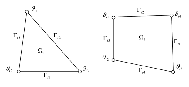
Figure 1: Two dimensional elements

3.2 A Godunov-type finite volume method

The first step is to integrate Eq. (1) over a finite volume element $\Omega_{i}$ yielding the following semi-discrete form for cell-average values.

$$\frac{d\overline{\bm{U}}_{i}}{dt}=\Re(\overline{\bm{U}}_{i})=-\frac{1}{\left|\Omega_{i}\right|}\oint_{\partial\Omega_{i}}\bm{F}_{n}(\bm{U})d\Gamma+\frac{1}{\left|\Omega_{i}\right|}\oint_{\Omega_{i}}\bm{S}d\Omega$$ (7)

where $\bm{F}_{n}(\bm{U})=\bm{F}(\bm{U})n_{ijx}+\bm{G}(\bm{U})n_{ijy}$. Curve integration along boundaries of the element can be calculated by the summation of integration along each edge.

$$\oint_{\partial\Omega_{i}}\bm{F}_{n}(\bm{U})d\Gamma=\sum_{j=1}^{J}\int_{\Gamma_{ij}}\bm{F}_{n}(\bm{U})d\Gamma\approx\sum_{j=1}^{J}\bm{F}_{nij}(\bm{U})\left|\Gamma_{ij}\right|=\sum_{j=1}^{J}\bm{F}_{nij}(\bm{U}_{ij}^{+},\bm{U}_{ij}^{-})\left|\Gamma_{ij}\right|$$ (8)

Here, $\bm{U}_{ij}^{\pm}$ are the right and left states at the edge $\Gamma_{ij}$. $\bm{F}_{nij}(\bm{U}_{ij}^{+},\bm{U}_{ij}^{-})$ is the numerical flux which can be calculated by Riemann solvers projected on the normal direction.

Finally, we can update cell-average values with the following third-order SSP Runge-Kutta [37] method.

$$\begin{array}[]{cc}\overline{\bm{U}}_{i}^{\ast}=\overline{\bm{U}}_{i}(t)+\triangle t\Re(\overline{\bm{U}}_{i}(t))\\ \overline{\bm{U}}_{i}^{\ast\ast}=\frac{3}{4}\overline{\bm{U}}_{i}(t)+\frac{1}{4}\overline{\bm{U}}_{i}^{\ast}+\frac{1}{4}\triangle t\Re(\overline{\bm{U}}_{i}^{\ast})\\ \overline{\bm{U}}_{i}(t+\triangle t)=\frac{1}{3}\overline{\bm{U}}_{i}(t)+\frac{2}{3}\overline{\bm{U}}_{i}^{\ast}+\frac{2}{3}\triangle t\Re(\overline{\bm{U}}_{i}^{\ast\ast})\end{array}$$ (9)

3.3 Reconstruction schemes

In this subsection, we propose two MUSCL-THINC/QQ-BVD schemes to reconstruct the left and right states $\bm{U}_{ij}^{\pm}$ from cell-averaged value $\overline{\bm{U}}_{i}$. A MUSCL scheme with the MLP-u2 limiter and the global THINC/QQ schemes with different steepness are implemented as reconstruction candidates. A BVD algorithm is then devised to select final reconstruction function from candidates. To avoid numerical oscillation, we choose primitive variables as reconstructed variables [38, 39], say, $(\rho,u,v,p)$ for the Euler equation and $(\alpha_{1},\alpha_{1}\rho_{1},\alpha_{2}\rho_{2},u,v,p)$ for the five-equation model. We denote a single reconstructed variable by $q$ to simplify the introduction.

3.3.1 The MUSCL scheme

The basic idea of a MUSCL-type scheme is to reconstruct variables in a certain cell by linear distributions. We use it as a candidate scheme in BVD schemes to approximate smooth solutions. For two dimensional unstructured grids, it can be written as,

$$q_{i}^{m}(x,y)=\bar{q}_{i}+\phi_{i}\left(q_{xi}(x-x_{ic})+q_{yi}(y-y_{ic})\right)$$ (10)

where $\bar{q}_{i}$ is the cell-average value, $\phi_{i}$ is a slope limiter to keep monotonicity and suppress numerical oscillation, $\left(q_{xi},q_{yi}\right)$ is the cell-averaged gradient determined from least-square method.

We use the so-called MLP-u2 limiter in [16] as the slope limiter for the MUSCL scheme.

$$\phi_{i}=\mathop{\min}\limits_{k=1}^{K}\left\{\begin{array}[]{ll}\Phi(R_{ik})&\textrm{if }\left(\overline{\nabla q}\right)_{i}\cdot\bm{r}_{ik}\neq 0\\ 1&\textrm{otherwise}\end{array}\right.$$

where $\bm{r}_{ik}(k=1,2,\dots,K)$ is the vector from $\vartheta_{ic}$ to vertex $\vartheta_{ik}$, and $R_{ik}$ is the ratio of the maximum or minimum allowable variation to the estimated variation at $\vartheta_{ik}$.

$$R_{ik}=\max\left(\frac{\bar{q}_{ik}^{min}-\bar{q}_{i}}{\left(\overline{\nabla q}\right)_{i}\cdot\bm{r}_{ik}},\frac{\bar{q}_{ik}^{max}-\bar{q}_{i}}{\left(\overline{\nabla q}\right)_{i}\cdot\bm{r}_{ik}}\right)$$

Here, $\bar{q}_{ik}^{min}$ and $\bar{q}_{ik}^{max}$ are minimum and maximum cell-average values of cells around $\vartheta_{ik}$. For the MLP-u2 limiter,

$$\Phi(R_{ik})=\frac{R_{ik}^{2}+2R_{i}k+\epsilon}{R_{ik}^{2}+R_{ik}+2.0+\epsilon}$$

where $\epsilon$ is a small positive number to distinguish a near smooth region from a fluctuating one. We take $\epsilon=1.0\times 10^{-15}$.

3.3.2 The THINC/QQ scheme

For unstructured grids, we use multi-dimensional THINC/QQ (THINC method with Quadratic surface representation and Gaussian Quadrature) scheme [34, 33] as another candidate in BVD schemes. As shown in [34, 33], THINC/QQ is able to achieve high accuracy discontinuity representation by accounting of geometrical information such as normal direction and curvature of the discontinuity. Here we use THINC/QQ in global coordinates, which states

$$q_{i}^{l}(x,y)=\bar{q}_{i}^{min}+\frac{\bar{q}_{i}^{max}-\bar{q}_{i}^{min}}{2}\left(1+\tanh\left(\frac{\beta}{H_{i}}\left(P_{i}(x,y)+d_{i}\right)\right)\right)$$ (11)

where $\bar{q}_{i}^{min}$ and $\bar{q}_{i}^{max}$ is the maximum and minimum cell-average values of cells sharing vertices with cell $\Omega_{i}$.

$$\bar{q}_{i}^{max}=\mathop{max}\limits_{k=1}^{K}\left\{\bar{q}_{ik}^{max}\right\},\bar{q}_{i}^{min}=\mathop{min}\limits_{k=1}^{K}\left\{\bar{q}_{ik}^{min}\right\}$$

$\beta$ is a parameter to control the steepness. $H_{i}$ is the hydraulic diameter of $\Omega_{i}$.

$$H_{i}=\frac{4\left|\Omega_{i}\right|}{\sum_{j=1}^{J}\left|\Gamma_{ij}\right|}$$

$P_{i}(x,y)+d_{i}$ is a full quadratic polynomial including geometrical information of the reconstruction as

$$P_{i}(x,y)=a_{20}(x-x_{ic})^{2}+a_{11}(x-x_{ic})(y-y_{ic})+a_{02}(y-y_{ic})^{2}+a_{10}(x-x_{ic})+a_{01}(y-y_{ic})$$

Coefficients $a_{st}(0<s+t\leq 2)$ can be calculated using least square method. The only unknown $d_{i}$ is determined from the conservation condition

$$\frac{1}{\left|\Omega_{i}\right|}\oint_{\Omega_{i}}q_{i}(x,y)dxdy=\bar{q}_{i}.$$

This integration is calculated with Gaussian quadrature. For more details, please refer to [34, 33].

3.3.3 The BVD algorithm

Generally, a numerical flux can be expressed in the following canonical formulation [26, 40]:

$$\bm{F}(\bm{U}_{L},\bm{U}_{R})=\frac{1}{2}\left(\bm{F}(\bm{U}_{L})+\bm{F}(\bm{U}_{R})\right)-\tilde{d}(\bm{U}_{R}-\bm{U}_{L}),$$ (12)

$\tilde{d}$ is a matrix function of $\bm{U}_{R}$ and $\bm{U}_{L}$. The last term of Eq.(12) can be interpreted as a diffusion term. The BVD algorithm is designed to select reconstruction function in target of minimizing the dissipation term. Choosing a final reconstruction with smaller boundary variation tends to preserve solution properties [41] and reduce numerical diffusion of the scheme.

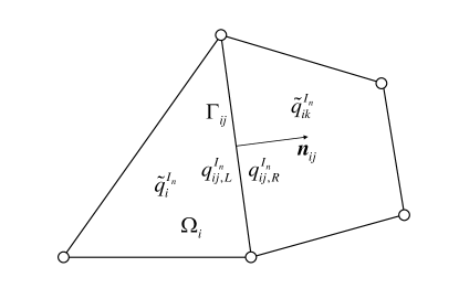
Figure 2: The left and right states of a cell face after reconstruction of candidate schemes

By assuming the target cell $i$ and its immediate neighbors are implemented with the same reconstruction scheme $I_{b}$ from the $B$ candidate schemes $(I_{1},I_{2},\cdots,I_{B})$, we define the BV at cell edge $\Gamma_{ij}$ as

$$BV_{ij}^{I_{b}}=\left|q_{ij,L}^{I_{b}}-q_{ij,R}^{I_{b}}\right|\left|\Gamma_{ij}\right|.$$

Then the total boundary variation ($TBV$) of cell $\Omega_{i}$ is defined as

$$TBV_{i}^{I_{b}}=\sum_{j=1}^{J}BV_{ij}^{I_{b}}.$$

Finally, the BVD algorithm selects the reconstruction scheme $I_{b}$ to reconstruct $q$ in cell $\Omega_{i}$ if $I_{b}$ satisfies the following condition

$$TBV_{i}^{I_{b}}=min(TBV_{i}^{I_{1}},TBV_{i}^{I_{2}},\cdots,TBV_{i}^{I_{B}}).$$

As shown later in numerical results, the proposed BVD algorithm is able to select jump-like THINC function for discontinuities thus to significantly improve resolution.

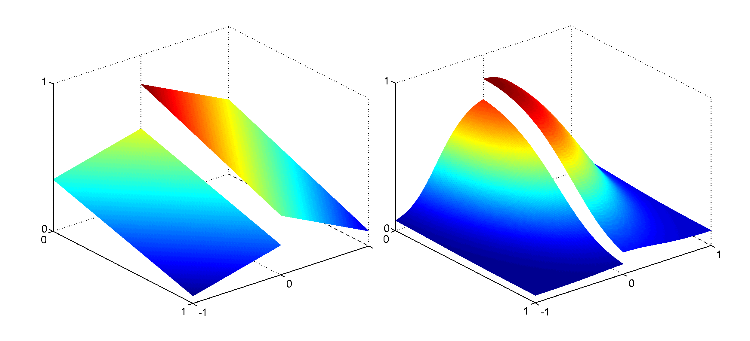
Figure 3: A illustration of possible reconstructions by the MUSCL scheme (left) and the THINC/QQ scheme (right)

3.3.4 The one-stage BVD scheme

Similar to the MUSCL-THINC-BVD scheme for structured grids, the one-stage BVD scheme has two candidate schemes: a MUSCL scheme and a THINC/QQ scheme with a relatively large steepness parameter $\beta_{l}$. The MUSCL scheme tends to smear discontinuities over several grids due to numerical dissipation. On the other hand, The THINC/QQ scheme can preserve the solution structure of discontinuities even for long-term simulations. Thus, using the BVD algorithm as the selecting procedure, we implement the MUSCL scheme at smooth regions and the THINC/QQ scheme at discontinuities. According to [30, 29] and our numerical tests, $\beta_{l}\sim(1.3,1.6)$ can give good or acceptable results and $\beta_{l}=1.4$ is used for all following test cases.

The one-stage BVD scheme is formulated as

$$q_{ij,\Theta}=\left\{\begin{array}[]{ll}q_{ij,\Theta}^{l}&\textrm{if }TBV_{i}^{l}<TBV_{i}^{m}\\ q_{ij,\Theta}^{m}&\textrm{otherwise}\end{array}\right.,\Theta=\left\{\begin{array}[]{ll}L&\textrm{if }\bm{n}_{ij}\textrm{ points outside of }\Omega_{i}\\ R&\textrm{otherwise}\end{array}\right.,j=1,2,\dots,J$$ (13)

where $TBV_{i}^{m/l}$ are $TBV$s corresponding to the MUSCL scheme and the THINC/QQ scheme with $\beta_{l}$.

Numerical tests show that this one-stage BVD scheme can efficiently reduce numerical diffusion at strong discontinuities such as shock waves and material interfaces. However, since a relatively large steepness $\beta_{l}$ is used, it can not capture some slight discontinuities such as shear waves and vortices.

3.3.5 The two-stage BVD scheme

The two-stage BVD scheme was inspired by a further investigation into the THINC/QQ scheme. Figure 3 shows possible reconstructions in two quadrilateral cells by the MUSCL scheme and the THINC/QQ scheme. As mentioned previously, The THINC/QQ function of Eq. 11 includes not only gradient terms but also curvature terms. Thus, it can preserve properties of some curved flow structures such as vortices better than the MUSCL scheme. To improve the performance of the one-stage BVD scheme at those curved smooth regions, and also for slight discontinuities, we add another THINC/QQ reconstruction with a relatively small steepness $\beta_{s}$ as the third candidate. According to [29] and our numerical tests, $\beta_{s}\sim(0.7,1.0)$ can give good or acceptable results. A $\beta_{s}=0.8$ is used for all the following test cases.

In the two-stage BVD scheme, we have three group of candidate states, say, $q_{ij,L/R}^{I}(I=m,s,l)$ from the MUSCL scheme, the THINC/QQ scheme with $\beta_{s}$ and the THINC/QQ scheme with $\beta_{l}$. The final reconstruction are chosen according to the following criterion.

$$q_{ij,\Theta}=\left\{\begin{array}[]{ll}q_{ij,\Theta}^{l}&\textrm{if }TBV_{i}^{l}<TBV_{i}^{m}\textrm{and }TBV_{i}^{l}<TBV_{i}^{s}\\ q_{ij,\Theta}^{s}&\textrm{if }TBV_{i}^{s}<TBV_{i}^{m}\textrm{and }TBV_{i}^{s}<TBV_{i}^{l}\\ q_{ij,\Theta}^{m}&\textrm{otherwise}\end{array}\right.,\Theta=\left\{\begin{array}[]{ll}L&\textrm{if }\bm{n}_{ij}\textrm{ points outside of }\Omega_{i}\\ R&\textrm{otherwise}\end{array}\right.,j=1,2,\dots,J$$ (14)

It is noticed that, this two-stage BVD algorithm is simpler than the one for structured grids in [31]. In fact, we compare all three $TBV$s directly and choose the scheme with the smallest $TBV$. This means that our two stages are parallel with a uniform algorithm. But for the structured one, two stages have a determined order to treat smooth regions and discontinuities separately.

4 Numerical results

4.1 Solid rotation of a complex profile

This case can assess the ability of present schemes to resolve sharp discontinuities and keep smooth regions smooth. We consider a complex 2D benchmark problem used by [42, 34] .The computational domain is $[0,1]^{2}$, divided into $54,604$ triangular elements. The initial condition consists three shapes within three circles of radius $r_{0}=0.15$ respectively, as showed in Figure 5.

$$\phi=\left\{\begin{array}[]{ll}1,\textrm{ if}\left|x-0.5\right|<0.25,\textrm{ or }y>0.85&r_{1}(x,y)<r_{0}\\ \frac{1}{4}(1+\textrm{cos}(\pi\textrm{min}(r_{2}(x,y)/r_{0},1)))&r_{2}(x,y)<r_{0}\\ 1-r_{3}(x,y)/r_{0}&r_{3}(x,y)<r_{0}\\ 0&\textrm{otherwise}\end{array}\right.$$

where $r_{i}(x,y)=\sqrt{(x-x_{i})^{2}+(y-y_{i})^{2}}$, $(x_{1},y_{1})=(0.5,0.78)$, $(x_{2},y_{2})=(0.31,0.39)$, $(x_{3},y_{3})=(0.69,0.39)$.

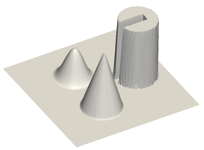
Figure 4: The initial condition of the rotation test

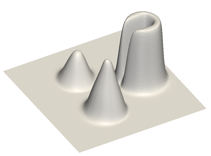
Figure 5: The solution of the MUSCL scheme

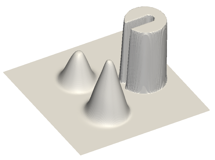
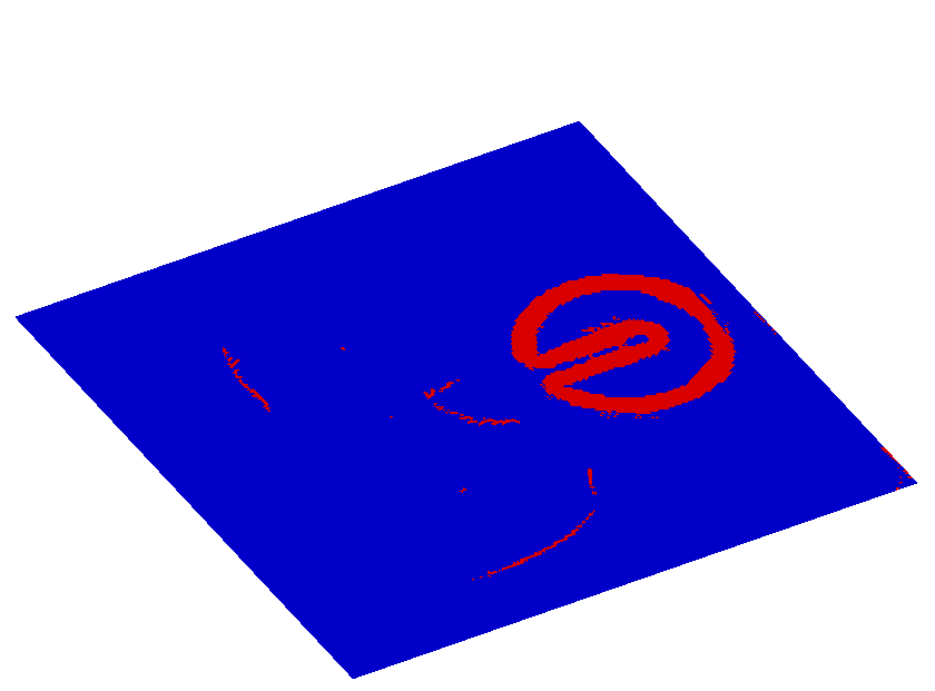
Figure 6: Results of the one-stage BVD scheme: (a)The solution after one rotation; (b)Red cells use THINC/QQ scheme

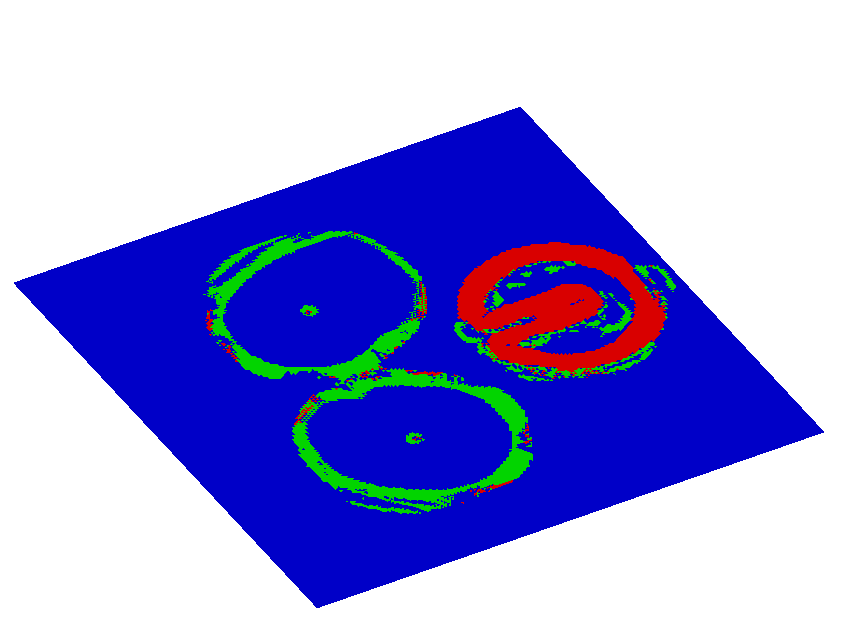
Figure 7: Results of the two-stage BVD scheme: (a)The solution after one rotation; (b)Red and yellow cells use THINC/QQ scheme

It includes a classical shape of a slotted disk proposed by Zalesak [43], a smooth hump and a sharp cone. These shapes are rotated by a velocity field of

$$u=0.5-y,v=x-0.5$$

Zero-gradient boundary condition is applied to all boundaries. Results of $t=2\pi$ by different schemes are showed in Figure 5 to 7. The maximum Courant number is set to $0.2$.

For the smooth hump and cone, three schemes give almost the same results. Since BVD schemes choose the MUSCL scheme for these region, as showed in Figure 6(b) and Figure 7(b). Although the two-stage BVD scheme chooses THINC/QQ scheme with $\beta_{s}$ in some cells (marked with yellow color) around hump and cone, it almost gives the same solution as the MUSCL scheme. On the other hand, BVD schemes can find cells including discontinuity (marked with red color), like the edge of the slotted disk, and implement THINC/QQ scheme with $\beta_{l}$ which can preserve the step-like solution structure. This step-like solution is smeared by the pure MUSCL scheme, as showed in Figure 5.

4.2 Gas Dynamic Problems

In this section, we assess the ability of BVD schemes to capture shock waves and vortices in gas dynamic problems. The Euler equation is solved by prescribed methods with the HLL Riemann solver. The ratio of specific heats is $\gamma=1.4$.

4.2.1 A Riemann Problem

Two-dimensional schemes are applied to a one-dimensional shock tube problem. The computational domain is $[0,1]\times[0,0.1]$ with $100$ triangular elements in the $x$-direction and $10$ triangular elements in the $y$-direction. We consider the following Riemann-type initial conditions [44]:

$$(\rho,u,p)=\left\{\begin{array}[]{ll}(1.0,0.0,1000.0)&\textrm{if }x<0.5\\ (1.0,0.0,0.01)&\textrm{otherwise}\end{array}\right.$$

It is the left half of the blast wave problem of Woodward and Colella [45]. Its solution contains a left rarefaction, a contact wave and a right-moving shock wave. Density of the exact solution and numerical methods at $t=0.012$ are showed in Figure 8. It is obvious that BVD schemes can resolve a sharper shock and contact wave than the pure MUSCL scheme, and there is no oscillation around discontinuities. Figure 9 shows cells using THINC/QQ schemes for reconstructing $\rho$ when BVD schemes are implemented. For cells around the shock and contact waves, the THINC/QQ with $\beta_{l}$ is used (red cells), which can preserve the step-like flow structure.

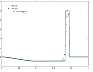
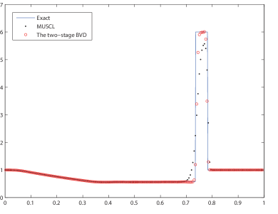
Figure 8: Density of the Riemann problem at $t=0.012$

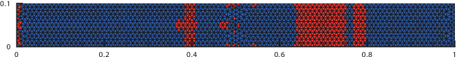
(a) The one-stage BVD scheme

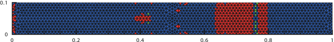
(b) The two-stage BVD scheme

Figure 9: Cells using THINC/QQ schemes to reconstruct density

4.2.2 A Mach 3 Wind Tunnel with a Step

This problem is also from [45], and widely used to verify the capability of numerical schemes in capturing strong shocks and vortices [46, 47, 19, 48, 49]. The wind tunnel is $1.0$ unit high and $3.0$ unit long. A step is located $0.6$ unit from the left boundary with a height of $0.2$ unit. This domain is divided into triangular elements with a size of $1/160$ away from the corner but $1/320$ around the corner, as Figure 10. This mesh was used by [46] to deal with the singularity point of the corner. The initial condition is the same as the inflow passing through the scram-jet engine.

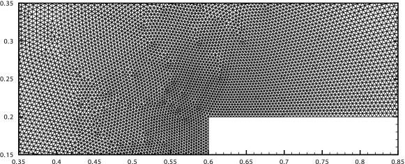
Figure 10: Mesh of wind tunnel around the corner

Figure 11 is the density contour at $t=4.0$, ranging from 0.32 to 6.15 with 30 equivalent intervals. It is seen that with the help of THINC/QQ schemes, BVD schemes can resolve shock waves better than pure MUSCL scheme. Red cells in FIgure 12 use THINC/QQ with $\beta_{l}$. They are also cells including shock waves. On the other hand, the two-stage BVD scheme can resolve very clear vortices, as showed in Figure 13. This benefits from the implementation of THINC/QQ with $\beta_{s}$, which also includes curvature information in second order terms but not as steep as the one with $\beta_{l}$. It can preserve flow structures of vortices. By comparing with the result of a 3rd-order WENO scheme [46], we can see that although the order of both the MUSCL scheme and the THINC/QQ scheme [33] are around 2nd-order, the combination of them by BVD algorithms can sometimes give better results than a 3rd-order scheme.

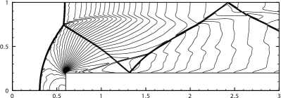
(a) The muscl scheme

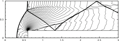
(b) The one-stage BVD scheme

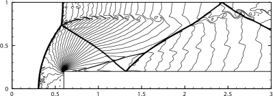
(c) The two-stage BVD scheme

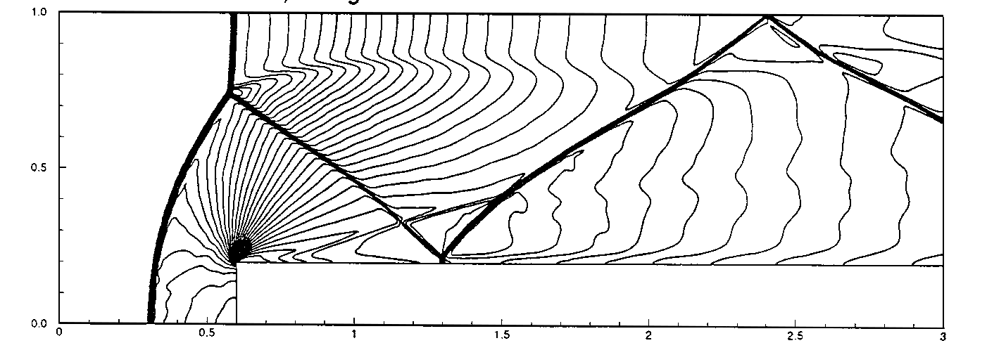
(d) The result of a 3rd-order scheme [46] with the same grid

Figure 11: Density contour of results at $t=4.0$

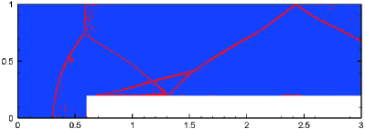
(a) The one-stage BVD scheme

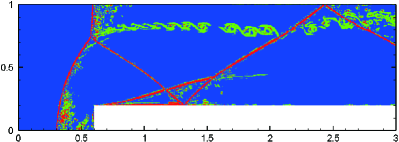
(b) The two-stage BVD scheme

Figure 12: Cells using THINC/QQ schemes to reconstruct $\rho$

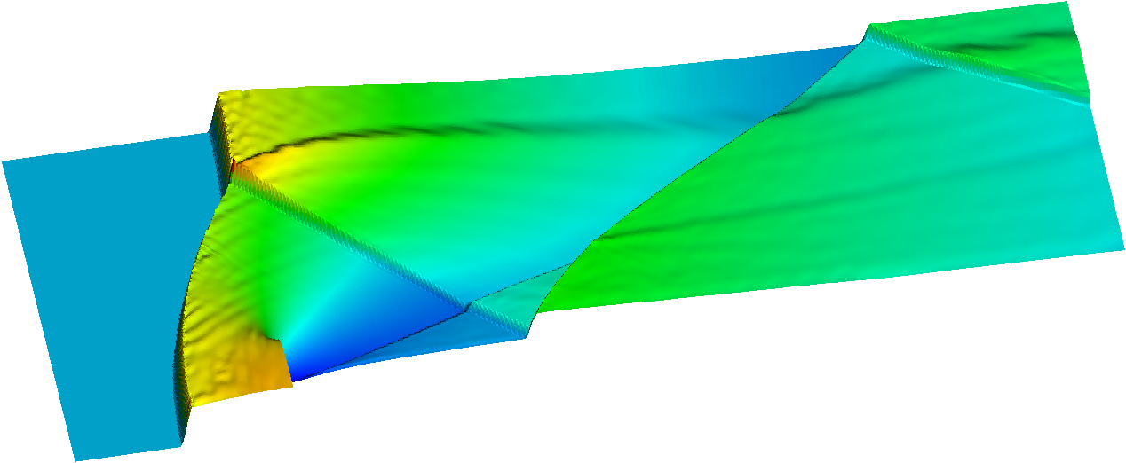
(a) The one-stage BVD scheme

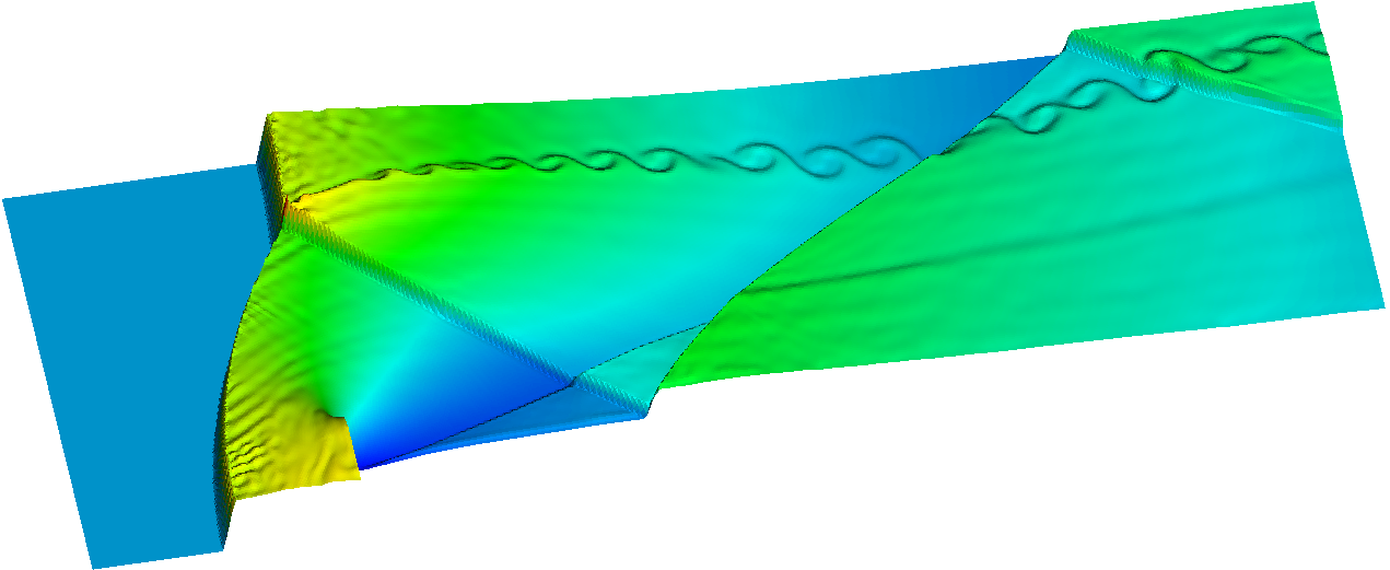
(b) The two-stage BVD scheme

Figure 13: Three-dimensional bird’s view of the density field

4.3 Two-fluid flow problems

One of main applications of the THINC scheme and the THINC/QQ scheme is to capture immersed interfaces. They can limit interfaces into several cells even over very long-term simulations [27, 33, 50, 51]. The combination of the THINC sheme and the MUSCL scheme by BVD algorithm in the structured-gird framework [30] showed that it can not only resolve a very clear interface, but also capture more flow details than traditional polynomial reconstructions such as the MUSCL scheme and the WENO sheme. In this section, we will see that the MUSCL-THINC/QQ-BVD scheme in the unstructured-grid framework has comparable performance. The five-equation model is solved by prescribed numerical schemes with the HLLC Riemann solver.

4.3.1 Two dimensional shock–R22-cylinder interaction

As the first benchmark test of two-component flows, we consider a well known shock-bubble interaction problem involving interaction between a shock in air and a R22 cylinder [30, 52, 53, 54, 55]. As analyzed in [56, 57], vortices will be generated by the baroclinic mechanism when the shock wave pass through the surface of R22 cylinder. Consider the equation of vorticity without viscous terms proposed in [56]:

$$\frac{d\bm{\omega}}{dt}+\bm{\omega}\nabla\cdot\bm{V}=\bm{\omega}\cdot\nabla\bm{V}+\frac{\nabla\rho\times\nabla p}{\rho^{2}}$$ (15)

The last term of Eq.(15) is a source term. Misalignment of the local gradient of pressure and local gradient of density will lead to a generation of vorticity. Figure 14 shows the direction of verticity generated in the interaction between a right-moving air shock and a R22 cylinder. If the numerical diffusion of a numerical scheme is too strong, it will smear these vortices.

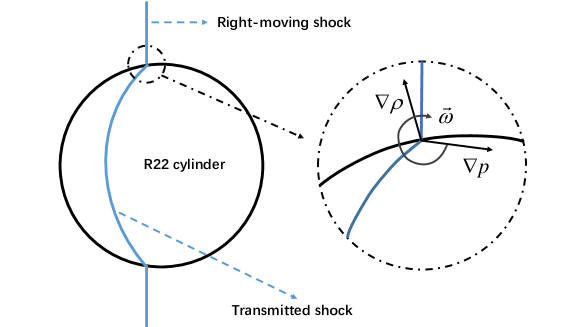
Figure 14: Generation of vorticity in interaction between air shock and R22 cylinder

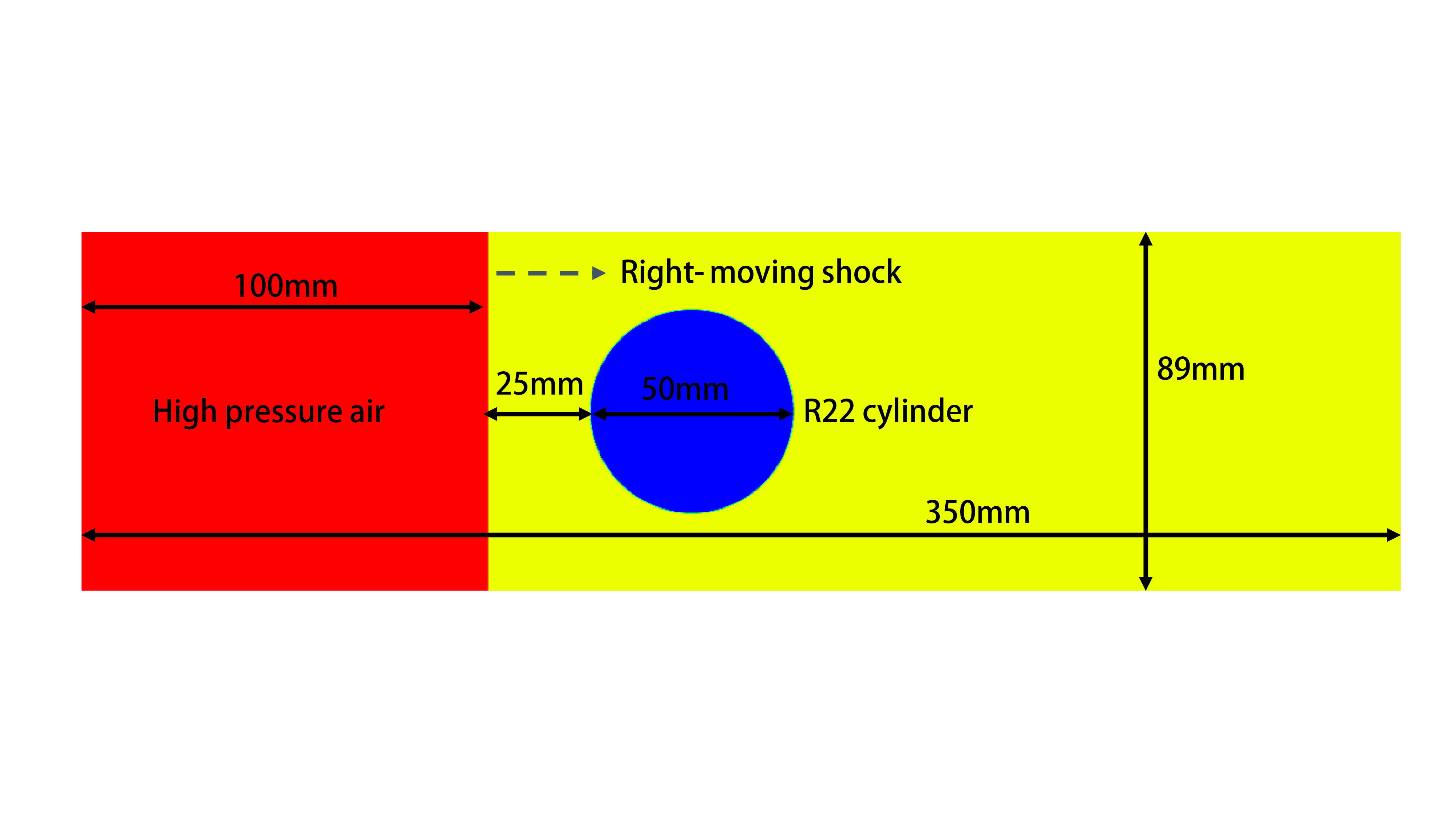
Figure 15: The computational domain of shock–R22-cylinder interaction

The computational setup is shown in Figure 15. Refer to [58] for experimental results. A planar right-moving Mach 1.22 shock in air hits a stationary R22 gas cylinder with a diameter $d=50mm$. Both air and R22 gas are treated as ideal gases. The initial condition is given as:

$$(\alpha_{1},\rho,u,v,p,\gamma)=\left\{\begin{array}[]{ll}(\epsilon,3.863kg/m^{3},0.0,0.0,1.01325\times 10^{5}Pa,1.249)&\textrm{In the R22 cylinder}\\ (1.0-\epsilon,1.686kg/m^{3},113.5m/s,0.0,1.59\times 10^{5}Pa,1.4)&\textrm{Post-shock}\\ (1.0-\epsilon,1.225kg/m^{3},0.0,0.0,1.01325\times 10^{5}Pa,1.4)&\textrm{Otherwise}\end{array}\right.$$

where $\epsilon=10^{-8}$. A uniform triangular mesh with $h=0.1875mm$ is used, which corresponds to a mesh number of 1,894,892. Reflective wall boundary conditions are implemented to the top and bottom boundaries. The left and right ones are zero gradient boundaries.

Numerical schlierens of results, $\ln(1.0+\left|\nabla\rho\right|)$, are shown in Figure 16 and 17. From the left column we can see that the one-stage BVD scheme can not only keep a very sharp interface, but also resolve vortices generated by the baroclinic mechanism. On the other hand, the MUSCL scheme is too diffusive that it smears almost all the small vortices. Only large-scale vortices can be observed in upper half of Figure 17 (a)(c)(e). Since Mach number of the shock wave is only 1.22, most wave structures generated by reflection and transmission are not strong enough to be distinguished by the one-stage BVD scheme. However, they can be recognised by the two-stage BVD scheme with both $\beta_{l}$ and $\beta_{s}$. At the same time, it is possible to reduce numerical dissipation further by the participation of the THINC/QQ scheme with $\beta_{s}$. That’s why interface of results by the two-stage BVD scheme have more small structures than those from the one-stage BVD scheme. Flow structures inside the R22 gas cylinder by BVD schemes are also clearer than the MUSCL scheme.

Finally we compare our results with those from the structured BVD scheme in [30]. Structured-grid framework can be done dimension-by-dimension without geometry dependence. For unstructured grids, we consider all the faces at the same time and including the geometry information of faces. Although there are some difference in detail, BVD schemes for two kind of grids share the same basic idea, say, reducing numerical diffusion by boundary variation diminishing. Thus, at least in our numerical tests, as showed in Figure 18, their behavior are very similar.

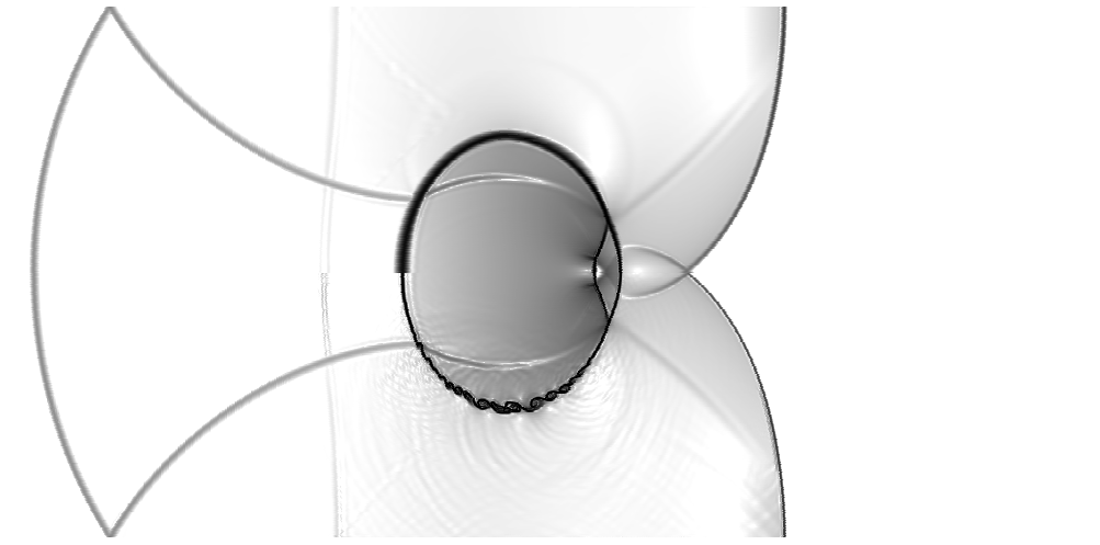
(a) $t=247\mu s$

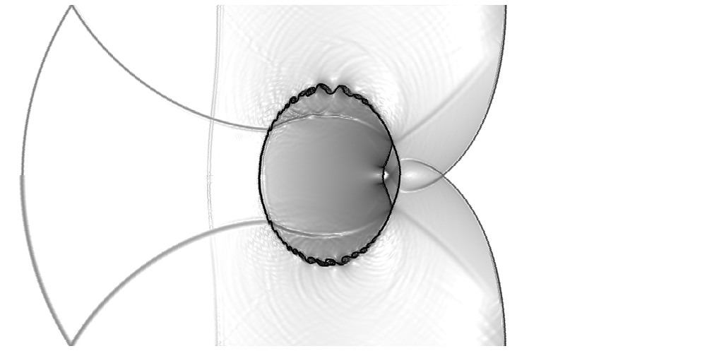
(b) $t=247\mu s$

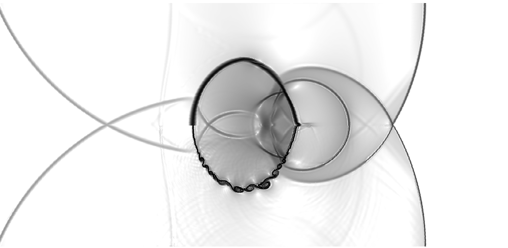
(c) $t=307\mu s$

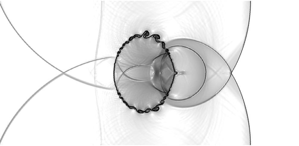
(d) $t=307\mu s$

Figure 16: Numerical schlierens for results of interaction between air shock and R22 cylinder. Pictures of each row are at the same instant. The result of the one-stage BVD (lower half) is plotted against results of MUSCL (left-upper half) and the two-stage BVD (right-upper half).

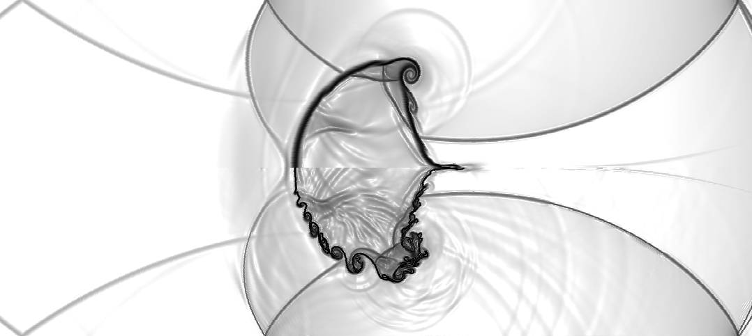
(a) $t=477\mu s$

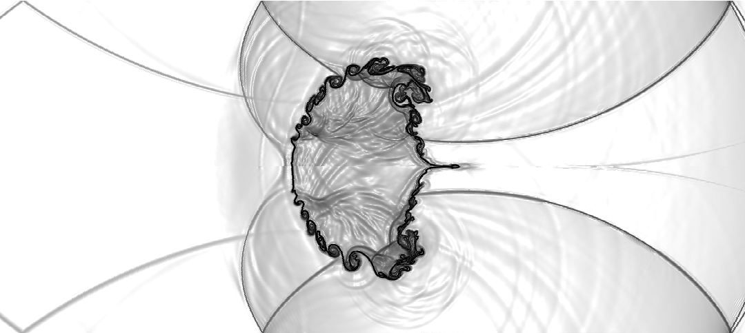
(b) $t=477\mu s$

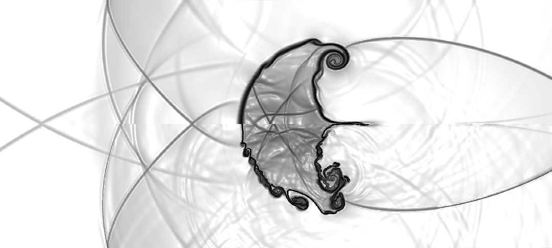
(c) $t=583\mu s$

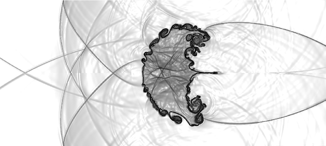
(d) $t=583\mu s$

Figure 17: Continue of Figure 16

(a) $t=378\mu s$

(b) $t=648\mu s$

Figure 18: Results from the two-stage BVD scheme (upper half) and [30] (lower half) with the same mesh number.

5 Conclusion remarks

In this work, we extend BVD algorithms of structured grids to unstructured grids by including geometrical information and propose two less-dissipate MUSCL-THINC/QQ-BVD schemes. Both of them can be implemented to reconstructed variables independently. Thus, they can be treated in the same manner as normal finite volume schemes. Results shows that our BVD algorithm can preserve solution properties and reduce numerical dissipation effectively. For advection or interface tracking problem, BVD schemes can limit discontinuities into few cells which can be controlled by parameter of steepness. In gas dynamic problems, both of the one- and two- stage BVD scheme can resolve sharp shock waves yet the MUSCL scheme tends to smear them. Numerical dissipation of the two-stage BVD scheme is further reduced at vortices and weak shocks. For compressible multi-component flows, the MUSCL scheme can not keep a clear material interface and resolve small flow structures induced by instabilities, but BVD schemes can capture them very clearly. Our results are comparable to results by the MUSCL-THINC-BVD scheme for structured grids. Furthermore, some of our results are even better than high-order finite volume schemes such as the fourth-order WENO scheme. This work shows that the basic idea of the BVD algorithm works very well for both structured and unstructured grids. It can be seen as another path to construct high-order non-oscillatory numerical schemes.

6 Acknowledgment

The authors acknowledge Dr. Peng Jin and Dr. Siengdy Tann at Tokyo Institute of Technology for their inspirational discussions. This paper was funded by International Graduate Exchange Program of Beijing Institute of Technology and National Natural Science Foundation of China (grant no. 11802178). FX was supported in part by the fund from JSPS (Japan Society for the Promotion of Science) under Grant Nos. 17K18838 and 18H01366.

References

- Barth and Frederickson [1990] T. Barth, P. Frederickson, Higher order solution of the euler equations on unstructured grids using quadratic reconstruction, in: 28th aerospace sciences meeting, 1990, p. 13.
- BARTH [1993] T. BARTH, Recent developments in high order k-exact reconstruction on unstructured meshes, in: 31st Aerospace Sciences Meeting, 1993, p. 668.
- Delanaye and Liu [1999] M. Delanaye, Y. Liu, Quadratic reconstruction finite volume schemes on 3d arbitrary unstructured polyhedral grids, in: 14th Computational Fluid Dynamics Conference, 1999, p. 3259.
- Reed and Hill [????] W. Reed, T. Hill, Triangular mesh methods for the neutron transport equation, technical report la-ur-73-479, los alamos scientific laboratory, los alamos, 1973 (????).
- Cockburn et al. [1990] B. Cockburn, S. Hou, C.-W. Shu, The runge-kutta local projection discontinuous galerkin finite element method for conservation laws. iv. the multidimensional case, Mathematics of Computation 54 (1990) 545–581.
- Huynh [2007] H. T. Huynh, A flux reconstruction approach to high-order schemes including discontinuous galerkin methods, in: 18th AIAA Computational Fluid Dynamics Conference, 2007, p. 4079.
- Vincent et al. [2011] P. E. Vincent, P. Castonguay, A. Jameson, A new class of high-order energy stable flux reconstruction schemes, Journal of Scientific Computing 47 (2011) 50–72.
- Castonguay et al. [2012] P. Castonguay, P. E. Vincent, A. Jameson, A new class of high-order energy stable flux reconstruction schemes for triangular elements, Journal of Scientific Computing 51 (2012) 224–256.
- Witherden et al. [2014] F. D. Witherden, A. M. Farrington, P. E. Vincent, Pyfr: An open source framework for solving advection–diffusion type problems on streaming architectures using the flux reconstruction approach, Computer Physics Communications 185 (2014) 3028–3040.
- Kopriva and Kolias [1996] D. A. Kopriva, J. H. Kolias, A conservative staggered-grid chebyshev multidomain method for compressible flows, Journal of computational physics 125 (1996) 244–261.
- Sun et al. [2006] Y. Sun, Z. Wang, Y. Liu, High-order multidomain spectral difference method for the navier-stokes equations, in: 44th AIAA Aerospace Sciences Meeting and Exhibit, 2006, p. 301.
- Harten [1983] A. Harten, High resolution schemes for hyperbolic conservation laws, Journal of computational physics 49 (1983) 357–393.
- Barth and Jespersen [1989] T. Barth, D. Jespersen, The design and application of upwind schemes on unstructured meshes, in: 27th Aerospace sciences meeting, 1989, p. 366.
- Spekreijse [1987] S. Spekreijse, Multigrid solution of monotone second-order discretizations of hyperbolic conservation laws, Mathematics of Computation 49 (1987) 135–155.
- Park et al. [2010] J. S. Park, S.-H. Yoon, C. Kim, Multi-dimensional limiting process for hyperbolic conservation laws on unstructured grids, Journal of Computational Physics 229 (2010) 788–812.
- Park and Kim [2012] J. S. Park, C. Kim, Multi-dimensional limiting process for finite volume methods on unstructured grids, Computers & Fluids 65 (2012) 8–24.
- Friedrich [1998] O. Friedrich, Weighted essentially non-oscillatory schemes for the interpolation of mean values on unstructured grids, Journal of computational physics 144 (1998) 194–212.
- Haselbacher [2005] A. Haselbacher, A weno reconstruction algorithim for unstructured grids based on explicit stencil construction, in: 43rd AIAA Aerospace Sciences Meeting and Exhibit, 2005, p. 879.
- Wolf and Azevedo [2007] W. Wolf, J. Azevedo, High-order eno and weno schemes for unstructured grids, International Journal for Numerical Methods in Fluids 55 (2007) 917–943.
- Titarev et al. [2010] V. Titarev, P. Tsoutsanis, D. Drikakis, Weno schemes for mixed-element unstructured meshes, Communications in Computational Physics 8 (2010) 585.
- Tsoutsanis et al. [2011] P. Tsoutsanis, V. A. Titarev, D. Drikakis, Weno schemes on arbitrary mixed-element unstructured meshes in three space dimensions, Journal of Computational Physics 230 (2011) 1585–1601.
- Persson and Peraire [2006] P.-O. Persson, J. Peraire, Sub-cell shock capturing for discontinuous galerkin methods, in: 44th AIAA Aerospace Sciences Meeting and Exhibit, 2006, p. 112.
- Barter and Darmofal [2010] G. E. Barter, D. L. Darmofal, Shock capturing with pde-based artificial viscosity for dgfem: Part i. formulation, Journal of Computational Physics 229 (2010) 1810–1827.
- Dumbser and Loubère [2016] M. Dumbser, R. Loubère, A simple robust and accurate a posteriori sub-cell finite volume limiter for the discontinuous galerkin method on unstructured meshes, Journal of Computational Physics 319 (2016) 163–199.
- Dumbser et al. [2014] M. Dumbser, O. Zanotti, R. Loubère, S. Diot, A posteriori subcell limiting of the discontinuous galerkin finite element method for hyperbolic conservation laws, Journal of Computational Physics 278 (2014) 47–75.
- Sun et al. [2016] Z. Sun, S. Inaba, F. Xiao, Boundary variation diminishing (bvd) reconstruction: A new approach to improve godunov schemes, Journal of Computational Physics 322 (2016) 309–325.
- Xiao et al. [2005] F. Xiao, Y. Honma, T. Kono, A simple algebraic interface capturing scheme using hyperbolic tangent function, International Journal for Numerical Methods in Fluids 48 (2005) 1023–1040.
- Jiang and Shu [1996] G.-S. Jiang, C.-W. Shu, Efficient implementation of weighted eno schemes, Journal of computational physics 126 (1996) 202–228.
- Deng et al. [2018a] X. Deng, B. Xie, R. Loubère, Y. Shimizu, F. Xiao, Limiter-free discontinuity-capturing scheme for compressible gas dynamics with reactive fronts, Computers & Fluids 171 (2018a) 1–14.
- Deng et al. [2018b] X. Deng, S. Inaba, B. Xie, K.-M. Shyue, F. Xiao, High fidelity discontinuity-resolving reconstruction for compressible multiphase flows with moving interfaces, Journal of Computational Physics 371 (2018b) 945–966.
- Deng et al. [2019] X. Deng, Y. Shimizu, F. Xiao, A fifth-order shock capturing scheme with two-stage boundary variation diminishing algorithm, Journal of Computational Physics 386 (2019) 323–349.
- Deng et al. [2020] X. Deng, Y. Shimizu, B. Xie, F. Xiao, Constructing higher order discontinuity-capturing schemes with upwind-biased interpolations and boundary variation diminishing algorithm, Computers & Fluids (2020) 104433.
- Xie and Xiao [2017] B. Xie, F. Xiao, Toward efficient and accurate interface capturing on arbitrary hybrid unstructured grids: The thinc method with quadratic surface representation and gaussian quadrature, Journal of Computational Physics 349 (2017) 415–440.
- Xie et al. [2019] B. Xie, X. Deng, S. Liao, F. Xiao, High-order multi-moment finite volume method with smoothness adaptive fitting reconstruction for compressible viscous flow, Journal of Computational Physics 394 (2019) 559 – 593.
- Allaire et al. [2002] G. Allaire, S. Clerc, S. Kokh, A five-equation model for the simulation of interfaces between compressible fluids, Journal of Computational Physics 181 (2002) 577–616.
- Shyue [2001] K.-M. Shyue, A fluid-mixture type algorithm for compressible multicomponent flow with mie–grüneisen equation of state, Journal of Computational Physics 171 (2001) 678–707.
- Gottlieb et al. [2001] S. Gottlieb, C.-W. Shu, E. Tadmor, Strong stability-preserving high-order time discretization methods, SIAM review 43 (2001) 89–112.
- Johnsen and Colonius [2006] E. Johnsen, T. Colonius, Implementation of weno schemes in compressible multicomponent flow problems, Journal of Computational Physics 219 (2006) 715–732.
- Johnsen [2011] E. Johnsen, On the treatment of contact discontinuities using weno schemes, Journal of Computational Physics 230 (2011) 8665 – 8668.
- Harten et al. [1983] A. Harten, P. D. Lax, B. v. Leer, On upstream differencing and godunov-type schemes for hyperbolic conservation laws, SIAM review 25 (1983) 35–61.
- Tann et al. [2019] S. Tann, X. Deng, Y. Shimizu, R. Loubère, F. Xiao, Solution property preserving reconstruction for finite volume scheme: a bvd+ mood framework, International Journal for Numerical Methods in Fluids (2019).
- LeVeque [1996] R. J. LeVeque, High-resolution conservative algorithms for advection in incompressible flow, SIAM Journal on Numerical Analysis 33 (1996) 627–665.
- Zalesak [1979] S. T. Zalesak, Fully multidimensional flux-corrected transport algorithms for fluids, Journal of computational physics 31 (1979) 335–362.
- Toro [2013] E. F. Toro, Riemann solvers and numerical methods for fluid dynamics: a practical introduction, Springer Science & Business Media, 2013.
- Woodward and Colella [1984] P. Woodward, P. Colella, The numerical simulation of two-dimensional fluid flow with strong shocks, Journal of computational physics 54 (1984) 115–173.
- Hu and Shu [1999] C. Hu, C.-W. Shu, Weighted essentially non-oscillatory schemes on triangular meshes, Journal of Computational Physics 150 (1999) 97–127.
- Li and Ren [2012] W. Li, Y.-X. Ren, High-order k-exact weno finite volume schemes for solving gas dynamic euler equations on unstructured grids, International Journal for Numerical Methods in Fluids 70 (2012) 742–763.
- Zhu et al. [2008] J. Zhu, J. Qiu, C.-W. Shu, M. Dumbser, Runge–kutta discontinuous galerkin method using weno limiters ii: unstructured meshes, Journal of Computational Physics 227 (2008) 4330–4353.
- Zhu and Qiu [2009] J. Zhu, J. Qiu, Hermite weno schemes and their application as limiters for runge-kutta discontinuous galerkin method, iii: unstructured meshes, Journal of Scientific Computing 39 (2009) 293–321.
- Shyue and Xiao [2014] K.-M. Shyue, F. Xiao, An eulerian interface sharpening algorithm for compressible two-phase flow: the algebraic thinc approach, Journal of Computational Physics 268 (2014) 326–354.
- Pandare et al. [2019] A. K. Pandare, H. Luo, J. Bakosi, An enhanced ausm+up scheme for high-speed compressible two-phase flows on hybrid grids, Shock Waves 29 (2019) 629–649.
- Quirk and Karni [1996] J. J. Quirk, S. Karni, On the dynamics of a shock–bubble interaction, Journal of Fluid Mechanics 318 (1996) 129–163.
- Shyue [2006] K.-M. Shyue, A wave-propagation based volume tracking method for compressible multicomponent flow in two space dimensions, Journal of Computational Physics 215 (2006) 219–244.
- Shankar et al. [2010] S. Shankar, S. Kawai, S. Lele, Numerical simulation of multicomponent shock accelerated flows and mixing using localized artificial diffusivity method, in: 48th AIAA Aerospace Sciences Meeting Including the New Horizons Forum and Aerospace Exposition, 2010, p. 352.
- So et al. [2012] K. So, X. Hu, N. A. Adams, Anti-diffusion interface sharpening technique for two-phase compressible flow simulations, Journal of Computational Physics 231 (2012) 4304–4323.
- Picone and Boris [1988] J. Picone, J. Boris, Vorticity generation by shock propagation through bubbles in a gas, Journal of Fluid Mechanics 189 (1988) 23–51.
- Giordano and Burtschell [2006] J. Giordano, Y. Burtschell, Richtmyer-meshkov instability induced by shock-bubble interaction: Numerical and analytical studies with experimental validation, Physics of Fluids 18 (2006) 036102.
- Haas and Sturtevant [1987] J.-F. Haas, B. Sturtevant, Interaction of weak shock waves with cylindrical and spherical gas inhomogeneities, Journal of Fluid Mechanics 181 (1987) 41–76.