Schur Polynomials through Lindström Gessel Viennot Lemma

Abstract

In this article, we use Lindström Gessel Viennot Lemma to give a short, combinatorial, visualizable proof of the identity of Schur polynomials — the sum of monomials of Young tableaux equals to the quotient of determinants. As a by-product, we have a proof of Vandermonde determinant without words. We also prove the cauchy identity. In the remarks, we discuss factorial Schur polynomials, dual Cauchy identity and the relation beteen Newton interpolation formula.

1 Introduction

The main purpose of this article is to give a combinatorial proof of the identity of Schur polynomials

$$\sum_{T\textrm{ Young tableaux}}x^{T}=\frac{\det(x_{i}^{\lambda_{j}+n-j})}{\det(x_{i}^{n-j})}$$

using this Lindström Gessel Viennot lemma. The classic algebraic proof, see Fulton and Harris [1] page 462, proving $\det(h_{\lambda_{i}+i-j})=\frac{\det(x_{i}^{\lambda_{j}+n-j})}{\det(x_{i}^{n-j})}$. The classic combinatorial proof (analysing a bijection carefully), see Mendes, and Remmel [3], page 40.

Lindström Gessel Viennot Lemma.

Let $\Gamma=(V,E)$ be a locally finite directed acyclic graph. Let $\{X_{e}:e\in E\}$ be a set of pairwise commutative indeterminants. For each path $P:v_{0}\stackrel{{\scriptstyle e_{1}}}{{\to}}v_{1}\to\cdots\stackrel{{\scriptstyle e_{k}}}{{\to}}v_{k}$, we define $X_{P}=X_{e_{1}}\cdots X_{e_{k}}$. For two vertices $u,v\in V$, we define $e(u,v)$ to be the sum of $X_{P}$ with $P$ going through all path from $u$ to $v$.

Now, fix some integer $n>0$, and two subsets of order $n$ of $V$, say $A=\{a_{1},\ldots,a_{n}\}$ and $B=\{b_{1},\ldots,b_{n}\}$. We have the following lemma.

Lemma 1 (Lindström Gessel Viennot Lemma, [2])

As notations above,

$$\det(e(a_{i},b_{j}))=\sum_{\sigma\in\mathfrak{S}_{n}}\operatorname{sgn}\sigma\sum_{\{P_{1},\ldots,P_{n}\}}X_{P_{1}}\cdots X_{P_{n}}$$

where $\{P_{1},\ldots,P_{n}\}$ goes through all pairwise non-intersecting paths with each $P_{i}$ from $a_{i}$ to $b_{\sigma(i)}$.

Schur polynomials.

For $n>0$, the $n$-variable Schur polynomial of a partition $\lambda:\lambda_{1}\geq\cdots\geq\lambda_{n}$ is defined to be

$$S_{\lambda}=\sum_{T}x^{T},$$

where $T$ goes through all Young tableaux (weakly increasing in row and strictly increasing in column) of alphabet $\{1,\cdots,n\}$ with shape $\lambda$. If we denote $N_{i}=\#T^{-1}\{i\}$, then $x^{T}$ is defined to be $x_{1}^{N_{1}}\cdots x_{n}^{N_{n}}$.

We know the following identity.

Theorem 2 (Jacobi-Trudy identity)

As notation above,

$$S_{\lambda}=\det(h_{\lambda_{i}+i-j}),$$

where $h_{k}$ is the sum of all monomials of degree $k$ in $n$ variables.

One of the combinatorial proof is to use Lindström Gessel Viennot lemma 1 above. Since we will use the proof of it, let me state the proof briefly.

Consider the lattice graph $\Gamma=(V,E)$, with $V=\mathbb{Z}\times\mathbb{Z}$ the plane lattice points, and $E$ all the edge from $(i,j)$ to $(i,j+1)$ and $(i+1,j)$. Assign the edge $(i,j)\to(i+1,j)$ by weight $x_{j}$, the rest by $1$, and consider

$$\begin{array}[]{l}A=\{a_{1}=(1,1),a_{2}=(2,1),\ldots,a_{n}=(n,1)\};\\ B=\{b_{1}=(1+\lambda_{n},n),b_{2}=(2+\lambda_{n-1},n),\ldots,b_{n}=(n+\lambda_{1},n)\}.\end{array}$$

Then the left hand side of Lindström Gessel Viennot Lemma is exactly $\det(h_{\lambda_{i}+i-j})$, and right hand side is exactly Schur polynomial. The proof is contained in wikipedia, [6]. For a complete proof, see for example Prasad [4].

2 Main Lemma

Here we consider the same graph $\Gamma=(V,E)$, the lattice graph, as above but of different weight. More precisely, assign the edge $(i,j)\to(i+1,j)$ by $x_{j}-x_{i+j}$, and the rest by $1$.

Lemma 3

Let $a=(1,1)$ and $b=(m,n)$, with $m,n>0$, then

$$e(a,b)=(x_{1}-x_{m+n-1})\cdots(x_{1}-x_{n+2})(x_{1}-x_{n+1}).$$

We use the convention that when $m+n-1<n+1$ the above expression equals to $1$.

This follows from induction. Firstly, the expression holds when $m=1$ or $n=1$. Generally, if $m,n>1$, let $b^{\prime}=(m-1,n)$ and $b^{\prime\prime}=(m,n-1)$, as below

Then

$$\begin{array}[]{rll}e(a,b)&=e(a,b^{\prime})(x_{n}-x_{m+n-1})+e(a,b^{\prime\prime})\\ &=(x_{1}-x_{m+n-2})\cdots(x_{1}-x_{n+2})(x_{1}-x_{n+1})(x_{n}-x_{m+n-1})\\ &+(x_{1}-x_{m+n-2})\cdots(x_{1}-x_{n+2})(x_{1}-x_{n+1})(x_{1}-x_{n})&\textrm{by induction}\\ &=(x_{1}-x_{m+n-1})\cdots(x_{1}-x_{n+2})(x_{1}-x_{n+1}).\end{array}$$

The proof is complete.

See figure 1 for first several terms.

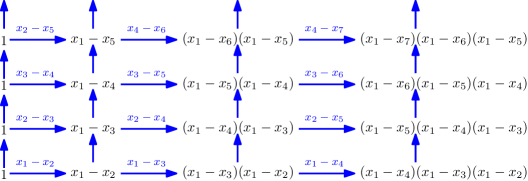
Figure 1: The table

Corollary 4

Let $a=(1,t)$ and $b=(m,n)$, with $m>s>0,n>t>0$. Then

$$e(a,b)=(x_{t}-x_{m+n-1})\cdots(x_{t}-x_{n+2})(x_{t}-x_{n+1}).$$

In particular, when $0=x_{n+1}=x_{n+2}=\cdots$, $e(a,b)=x_{t}^{m-1}$.

By replacing $(x_{1},x_{2},\ldots)$ by $(x_{t},x_{t+1},\ldots)$.

As an application, we can get the classic Vandermonde determinant from above computation and Lindström Gessel Viennot Lemma 1.

Theorem 5 (Vandermonde)

For $n$ variables, the determinant $\det(x_{i}^{n-j})=\prod_{i<j}(x_{i}-x_{j})$.

Consider the graph above, with $0=x_{n+1}=x_{n+2}=\cdots$ and consider

$$\begin{array}[]{l}A=\{a_{1}=(1,1),a_{2}=(1,2),\cdots,a_{n}=(1,n)\}\\ B=\{b_{1}=(n,n),b_{2}=(n-1,n),\cdots,b_{n}=(1,n)\}\end{array}$$

Then by 4 above $e(a_{i},b_{j})=x_{i}^{n-j}$. But the only non-intersecting paths are as figure 2. Apply Lindström Gessel Viennot Lemma 1, we see $\det(x_{i}^{n-j})=\prod_{i<j}(x_{i}-x_{j})$.

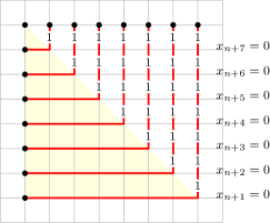
Figure 2: Prove Vandermonde determinant without words

3 Schur polynomial by quotient of determinants

Theorem 6

The $n$-variable Schur polynomial of a partition $\lambda:\lambda_{1}\geq\cdots\geq\lambda_{n}$

$$S_{\lambda}=\frac{\det(x_{i}^{\lambda_{j}+n-j})}{\det(x_{i}^{n-j})}.$$

Step 1. Remind the proof of Jacobi Trudy identity 2. Since the path from $(i,1)$ in any set of non-intersecting paths only went vertically before height $n-i+1$, so it is equivalent to change $(i,1)$ by $a_{i}^{\prime}=(i,n-i+1)$. That is,

$$\det(e(a^{\prime}_{i},b_{j}))=S_{\lambda}.$$

See figure 3.

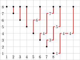
Figure 3: First step of reduction

Now, if we apply $0=x_{n+1}=x_{n+2}=\cdots$ in the weight of last section, then in the region $\{(i,j):i+j\geq n\}$, it coincides with that in the proof of Jacobi Trudy identity 2.

Step 2. Let us consider $a_{i}^{\prime\prime}=(1,n-i+1)$. It is easy to see

$$e(a_{i}^{\prime\prime},b_{j})=\sum_{k}e(a_{i}^{\prime\prime},a_{k}^{\prime})\cdot e(a_{k}^{\prime},b_{j}),$$

so

$$\det(e(a_{i}^{\prime\prime},b_{j}))=\det(e(a_{i}^{\prime\prime},a_{j}^{\prime}))\cdot\det(e(a_{i}^{\prime},b_{j})).$$

And trivially,

$$\det(e(a_{i}^{\prime\prime},a_{j}^{\prime}))=\prod_{i<j}(x_{i}-x_{j})=\det(x_{i}^{n-j}),$$

the Vandermonde determinant 5. See figure 4.

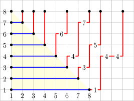
Figure 4: Second step of reduction

Step 3. By corollary 4, $e(a_{n+1-i}^{\prime\prime},b_{n+1-j})=x_{i}^{\lambda_{j}+n-j}$, so

$$\det(e(a_{i}^{\prime\prime},b_{j}))=\det(x_{i}^{\lambda_{j}+n-j})$$

See figure 5.

Hence the equation $(1,2,3,4)$ proves the assertion.

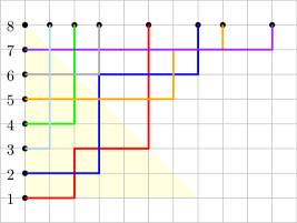
Figure 5: Last step of reduction

4 Cauchy identity

We can use the identical way to prove Cauchy identity.

Theorem 7 (Cauchy)

For fixed $n>0$, and $x_{1},\ldots,x_{n},y_{1},\ldots,y_{n}$ two sets of variables,

$$\frac{1}{\prod_{i<j}(x_{i}-x_{j})\prod_{i<j}(y_{i}-y_{j})}\det\left(\frac{1}{1-x_{i}y_{j}}\right)=\sum_{\lambda}S_{\lambda}(x)S_{\lambda}(y),$$

with $\lambda$ going through all young diagrams with no more than $n$ rows.

Here we consider a variant of our graph. Consider the graph $\Gamma=(V,E)$,

$$V=\{1,2,3,\ldots\}\times\{1,2,\cdots,2n-1,2n\}$$

with edge $(i,j)\to(i,j+1)$ with weight $1$, and $(i,j)\to(i+1,j)$ of weight $x_{j}-x_{i+j}$ if $j\leq n$, $(i+1,j)\to(i,j)$ of weight $y_{2n-j}-y_{i+2n-j}$ if $j\geq n+1$. Then apply $0=x_{n+1}=x_{n+2}=\cdots$ and $0=y_{n+1}=y_{n+2}=\cdots$. Consider the points

$$a_{1}=(1,1),a_{2}=(1,2),\cdots,a_{n}=(1,n)$$

and

$$b_{n}=(1,n+1),b_{n-1}=(1,n+2),\cdots,b_{1}=(1,2n).$$

Then cutting the line $y=n+1/2$, by corollary 4 we see (see figure 6)

$$e(a_{i},b_{j})=\sum_{k=0}^{\infty}x_{i}^{k}y_{j}^{k}=\frac{1}{1-x_{i}y_{j}}.$$

Apply Lindström Gessel Viennot Lemma 1. By the same argument of cut, we see the right hand side is actually $\sum_{\lambda}S_{\lambda}(x)S_{\lambda}(y)$, see figure 7. The proof is complete.

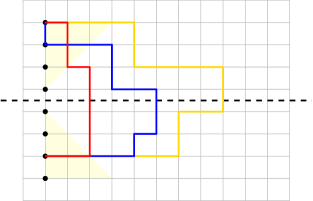
Figure 6: Cutting the line $y=n+1/2$

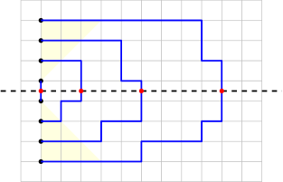
Figure 7: Cutting the line $y=n+1/2$

Actually, the left hand side of above identity turns out to be $\prod_{i,j=1}^{n}\frac{1}{1-x_{i}y_{j}}$, known as Cauchy determinant.

For the classic proof, see Richard and Sergey [5] theorem 7.12.1, using Robinson Schensted Knuth Algorithm.

5 Remarks

Factorial Schur polynomials.

Firstly, there are also factorial Schur polynomials

$$S_{\lambda}(x\mid a)=\sum_{T}\prod_{(i,j)\in\lambda}(x_{T(i,j)}-a_{T(i,j)+i-j})$$

with $A$ going through all Young tableaux of $\lambda$. By a completely same argument, but $x_{n+i}=a_{i}$,

$$S_{\lambda}(x\mid a)=\frac{\det[(x_{j}\mid a)^{\lambda_{i}+n-i}]}{\det(x_{i}^{n-j})}$$

with $(y\mid a)^{k}=(y-a_{1})...(y-a_{k})$.

Dual Cauchy identity.

Secondly, there is also dual Cauchy identity,

$$\prod_{i=1}^{n}\prod_{j=1}^{m}(1+x_{i}y_{j})=\sum_{\lambda}S_{\lambda}(x)S_{\lambda^{\prime}}(y)$$

where $\lambda$ goes through all young diagrams of at lost $n$ rows and $m$ columns, and $\lambda^{\prime}$ is the conjugation of $\lambda$. The classic proof, see Richard and Sergey [5] theorem 7.14.3, using dual Robinson Schensted Knuth Algorithm. This can be proven like what we did in proof of Cauchy identity 7 but a little careful about the sign. More precisely, consider the graph $\Gamma=(V,E)$,

$$V=\{1,2,3,\cdots,m+n\}\times\{1,2,3\cdots,m+n-1\}$$

with edge $(i,j)\to(i,j+1)$ with weight $1$, and $(i,j)\to(i+1,j)$ of weight $x_{j}-x_{i+j}$ if $j\leq n$, $(i,j)\to(i+1,j)$ of weight $-(y_{m+n-j}-y_{(m+n-i)+(m+n-j)})$ if $j\geq n+1$. Similar, we apply $0=x_{n+1}=x_{n+2}=\cdots$ and $0=y_{m+1}=y_{m+2}=\cdots$ Then consider

$$(1,1),(1,2),\ldots,(1,n),\quad(m+n,n),(m+n,n+1),\ldots,(m+n,m+n-1)$$

and

$$(1,n),(2,n),\ldots,(m+n,n).$$

See figure 8. The sign of permutation cancels the sign of $y_{\bullet}$’s. Apply Lindström Gessel Viennot Lemma, 1, the left hand side is

$$\det\left(\begin{matrix}x_{1}^{m+n-1}&\cdots&x_{n}^{m+n-1}&(-y_{1})^{0}&\cdots&(-y_{m})^{0}\\ \vdots&\ddots&\vdots&\vdots&\ddots&\vdots\\ x_{1}^{0}&\cdots&x_{n}^{0}&(-y_{n})^{m+n-1}&\cdots&(-y_{m})^{m+n-1}\end{matrix}\right)$$

and the right hand side is

$$\prod_{1\leq i<j\leq n}(x_{i}-x_{j})\prod_{1\leq i<j\leq m}(y_{i}-y_{j})\sum_{\lambda}S_{\lambda}(x)S_{\lambda^{\prime}}(y).$$

By a direct computation of $(*)$ (a good exercise of linear algebra), we get dual Cauchy identity.

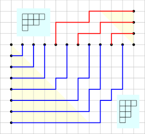
Figure 8: Dual Cauchy identity

Newton interpolation formula.

Last but no mean least, our weight chosen is relative to Newton interpolation formula. If we view $x_{0}=x$ as variable, and $x_{1},x_{2},\ldots,x_{n}$ as data points, as usual $0=x_{n+1}=x_{n+2}=\cdots$. Cutting the path from $(1,0)$ to $(n,n)$ by $y=\frac{1}{2}$, see figure 9, by corollary 4, we have the following identity

$$\begin{array}[]{rl}x^{n}&=e(a_{0},b)\\ &\quad+e(a_{1},b)\cdot(x-x_{1})\\ &\qquad+e(a_{2},b)\cdot(x-x_{1})(x-x_{2})+\cdots\\ &\qquad\quad+e(a_{n},b)\cdot(x-x_{1})\cdots(x-x_{n}),\end{array}$$

with $a_{i}=(i,1)$, $N=(n,n)$.

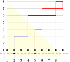
Figure 9: Newton interpolation formula

One can show by induction that for each point $(i,j)$ with $0\leq i,j\leq n$, $e((i,j),b)$ corresponds to a divided differences of $x^{n}$. More exactly, consider the inverse diagram, and stare at the following diagram.

Since $\heartsuit\cdot(x_{1}-x_{2})+x_{2}^{n}=x_{1}^{n}$, so $\heartsuit=\frac{x_{1}^{n}-x_{2}^{n}}{x_{1}-x_{2}}$. The same reason, $\diamondsuit=\frac{x_{2}^{2}-x_{3}^{n}}{x_{2}-x_{3}}$. Therefore $\square=\frac{\heartsuit-\diamondsuit}{x_{1}-x_{3}}$, and so on.

References

- [1] William Fulton and Joe Harris. Representation theory. A first course., volume 129. New York etc.: Springer-Verlag, 1991.
- [2] Ira M Gessel and Xavier Viennot. Determinants, paths, and plane partitions. preprint, 132(197.15), 1989.
- [3] Anthony Mendes and Jeffrey Remmel. Counting with symmetric functions. Springer, 2015.
- [4] Amritanshu Prasad. An introduction to schur polynomials. 2018.
- [5] Richard P. Stanley and Sergey Fomin. Enumerative Combinatorics, volume 2 of Cambridge Studies in Advanced Mathematics. Cambridge University Press, 1999.
- [6] Wikipedia contributors. Lindström–gessel–viennot lemma — Wikipedia, the free encyclopedia, 2019. [Online; accessed 19-March-2020].