New statistical model for misreported data with application to current public health challenges

Abstract

The main goal of this work is to present a new model able to deal with potentially misreported continuous time series. The proposed model is able to handle the autocorrelation structure in continuous time series data, which might be partially or totally underreported or overreported. Its performance is illustrated through a comprehensive simulation study considering several autocorrelation structures and two real data applications on human papillomavirus incidence in Girona (Catalunya, Spain) and Covid-19 incidence in the Chinese region of Heilongjiang.

1 Introduction

There has been a growing interest in the past years to deal with data that is only partially registered or underreported in the time series literature. This phenomenon is very common in many fields, and has been previously explored by different approaches in epidemiology, social and biomedical research among many other contexts [6, 3, 23, 1, 27]. The sources and underlying mechanisms that cause the underreporting might differ depending on the particular data. Some authors consider a situation where the registry is updated with time and therefore the underreporting issue is mitigated [13]. That leads to temporary underreporting while this work is focused on permanent underreporting, where the registered data are never updated in order to become more accurate. From the methodological point of view, several alternatives have been explored, from Markov chain Monte-Carlo based methods [27] to recent discrete time series approaches [9, 10]. Several attempts to estimate the degree of underreporting in different contexts have been done [11], although there is a lack of models incorporating continuous time series structures and handling underreporting.

One of the fields where the interest in addressing the underreporting issues is higher is the epidemiology of infectious diseases. In the last few years, many approaches to deal with underreported data have been suggested with a growing level of sophistication from the usage of multiplication factors [25] to several Markov-based models [4, 20] or even spatio-temporal modelling [26]. Even a new R [22] package able to fitting endemic-epidemic models based on approximative maximum likelihood to underreported count data has been recently published [17]. This work presents two examples where such phenomenon appears.

Human papillomavirus (HPV) is one of the most prevalent sexually transmitted infections. It is so common that nearly all sexually active people have it at some point in their lives, according to the information provided by the United States’ Centers for Disease Control and Prevention (CDC) [8]. Generally, the infection disappears on its own without inducing any health problem, but in some cases it can produce an abnormal growth of cells on the surface of the cervix that could potentially lead to cervical cancer. HPV infection is also related to other cancers (vulva, vagina, penis, anus, $\dots$) and other diseases like genital warts (GW). The fact that most cases of HPV infection are asymptomatic causes that public health registries might be potentially underestimating its incidence. The underreporting phenomenon in HPV data from the discrete time series point of view has been recently studied [9].

There is an enormous global concern around 2019-novel coronavirus (SARS-CoV-2) infection in the last few months, leading the World Health Organization (WHO) to declare public health emergency [24]. As the symptoms of this infection can be easily confused with those of similar diseases like Middle East Respiratory Syndrome Coronavirus (MERS-CoV) or Severe Acute Respiratory Syndrome Coronavirus (SARS-CoV), its incidence has been notably underreported, especially at the beginning of the outbreak in Wuhan (Hubei province, China) by December 2019.

2 Model definition

Consider an unobservable process with an AutoRegressive Moving Average ($ARMA(p,r)$) structure defined by

$$X_{t}=\alpha_{1}X_{t-1}+\ldots+\alpha_{p}X_{t-p}+\theta_{1}\epsilon_{t-1}+\ldots+\theta_{r}\epsilon_{t-r}+\epsilon_{t},$$ (1)

where $\epsilon_{t}$ is a Gaussian white noise process with $\epsilon_{t}\sim N(\mu_{\epsilon},\sigma_{\epsilon}^{2})$. The ARMA processes belong to the family of so called linear processes. Their importance relies on the fact that any stationary nondeterministic process can be written as a sum of a linear process and a deterministic component [7]. These models are very well known, have been used in many applications since their introduction in the early 1950’s and are general and flexible enough to be useful in a wide range of different contexts. Most used statistical software packages include functions that allow straightforward fitting of this family of models, so it seems a natural choice in the present work.

In our setting, this process $X_{t}$ cannot be directly observed, and all we can see is a part of it, expressed as

$$Y_{t}=\left\{\begin{array}[]{ll}X_{t}\text{ with probability }1-\omega\\ q\cdot X_{t}\text{ with probability }\omega\end{array}\right.$$ (2)

The interpretation of the parameters in Eq. (2) is straightforward: $q$ is the overall intensity of misreporting (if $0<q<1$ the observed process $Y_{t}$ would be underreported while if $q>1$ the observed process $Y_{t}$ would be overreported). The parameter $\omega$ can be interpreted as the overall frequency of misreporting (proportion of misreported observations).

2.1 Model properties

Consider that the unobserved process $X_{t}$ follows an $ARMA(p,r)$ model as defined in Eq. (1). As can be seen in Appendix 1 (Supplementary Material), the observed process has mean $\mathbb{E}(Y_{t})=\frac{\mu_{\epsilon}}{1-\alpha_{1}-\ldots-\alpha_{p}}\cdot\left(1-\omega+q\cdot\omega\right)$ and variance $\mathbb{V}(Y_{t})=\left(\left(\frac{\sigma_{\epsilon}^{2}\cdot(1+\theta_{1}^{2}+\ldots+\theta_{r}^{2})}{1-\alpha_{1}^{2}-\ldots-\alpha_{p}^{2}}\right)+\frac{\mu^{2}_{\epsilon}}{(1-\alpha_{1}-\ldots-\alpha_{p})^{2}}\right)\cdot(1+\omega\cdot(q^{2}-1))-\frac{\mu^{2}_{\epsilon}}{(1-\alpha_{1}-\ldots-\alpha_{p})^{2}}\cdot(1-\omega+q\cdot\omega)^{2}$. The autocorrelation function of the observed process can be written in terms of the features of the hidden process $X_{t}$ as

$$\begin{array}[]{ll}\rho_{Y}(k)&=\frac{V(X_{t})(1-\omega+q\omega)^{2}}{(V(X_{t})+E(X_{t})^{2})(1+\omega(q^{2}-1))-E(X_{t})^{2}(1-\omega+q\cdot\omega)^{2}}\cdot\rho_{X}(k)=\\ &=c(\alpha_{1},\ldots,\alpha_{p},\theta_{1},\ldots,\theta_{r},\mu_{\epsilon},\sigma^{2}_{\epsilon},\omega,q)\cdot\rho_{X}(k),\end{array}$$ (3)

where $\rho_{X}$ is the autocorrelation function of the unobserved process $X_{t}$.

A situation of particular interest is the case $\omega=1$, meaning that all the observations might be underreported and that a simpler model for $Y_{t}$ excluding the parameter $\omega$ might be suitable

$$Y_{t}=q\cdot X_{t}.$$ (4)

In this case, however, the observed process $Y_{t}$ would be a non-identifiable $ARMA(p,r)$ model as the parameter $q$ cannot be estimated on the basis of the methodology described in the following section.

2.2 Estimation

The likelihood function of the observed process $Y_{t}$ is not easily computable but the parameters of the model can be estimated by means of an iterative algorithm based on its marginal distribution, using the R packages mixtools [5] and forecast [16, 15]. The main steps are described in detail below:

1. Following Eq. (2), the observed process $Y_{t}$ can be written as $Y_{t}=(1-Z_{t})\cdot X_{t}+q\cdot Z_{t}\cdot X_{t}$, where $Z_{t}$ is an indicator of the underreported observations, following a Bernoulli distribution with probability of success $\omega$ $(Z_{t}\sim Bern(\omega))$. The marginal distribution of $Y_{t}$ is a mixture of two normal random variables $N\left(\mu,\sigma^{2}\right)$ and $N\left(q\cdot\mu,q^{2}\cdot\sigma^{2}\right)$ respectively, where $\mu=\frac{\mu_{\epsilon}}{1-\alpha_{1}-\ldots-\alpha_{p}}$ and $\sigma^{2}=\frac{\sigma_{\epsilon}^{2}\cdot(1+\theta_{1}^{2}+\ldots+\theta_{r}^{2})}{1-\alpha_{1}^{2}-\ldots-\alpha_{p}^{2}}$. This fact can be used to obtain initial estimates for $q$ and $\omega$. Using the EM algorithm (specifically on the E-step), the posterior probabilities (conditional on the data and the obtained estimates) can be computed. This can be done using, for instance, the R package mixtools.

2. Using the indicator $\hat{Z_{t}}$ obtained in the previous step, the series is divided in two: One including the underreported observations (treating the non-underreported values as missing data) and another with the non underreported observations (treating the underreported values as missing data). An $ARMA$ model is fitted to each of these two series and a new $\hat{q}$ is obtained by dividing the fitted means.

3. A mixture of two normals is fitted to the observed series $Y_{t}$ with mean and standard deviation fixed to the corresponding values obtained from the previous step, and a new $\omega$ is estimated.

4. Steps (ii) and (iii) are repeated until the quadratic distance between two consecutive iterations $(\hat{q}_{i}-\hat{q}_{i-1})^{2}+(\hat{\omega}_{i}-\hat{\omega}_{i-1})^{2}+\sum_{j}(\hat{\alpha}_{j_{i}}-\hat{\alpha}_{j_{i-1}})^{2}+\sum_{k}(\hat{\theta}_{k_{i}}-\hat{\theta}_{k_{i-1}})^{2}$ is below a fixed tolerance level.

5. Once the parameter estimates are stable according to the previous criterion, the underlying process $X_{t}$ is reconstructed as $\hat{X_{t}}=(1-\hat{Z_{t}})\cdot Y_{t}+\frac{1}{\hat{q}}\cdot\hat{Z_{t}}\cdot Y_{t}$, and an $ARMA$ model is fitted to the reconstructed process to obtain $\hat{\alpha}_{j}$, $j=1,\ldots,p$, $\hat{\theta}_{k}$, $k=1,\ldots,r$ and $\hat{\sigma_{\epsilon}}^{2}$.

To account for potential trends or seasonal behaviour, covariates can be included in the described estimation process. Additionally, a parametric bootstrap procedure with 500 replicates is used to estimate standard errors and build confidence intervals based on the percentiles of the distribution of the estimates. The R codes used to estimate the parameters and build the confidence intervals are available from the authors upon request.

3 Results

The results of the proposed methodology over a comprehensive simulation study and an application on two real data sets are shown in this Section.

3.1 Simulation study

A thorough simulation study has been conducted to ensure that the model behaves as expected, including $AR(p)$, $MA(r)$ and $ARMA(p,r)$ for $1\leq p,r\leq 3$ structures for the hidden process $X_{t}$ with values for the parameters $\alpha$, $\theta$, $q$ and $\omega$ ranging from 0.1 to 0.9 for each parameter (some combinations of parameters have been omitted for $p>1$ or $r>1$ to ensure stationarity). For $ARMA(p,r)$ structures with $p>1$ or $r>1$ the parameters covered the same range (0.1 to 0.9) but with a difference of 0.2 instead of 0.1 for computational feasibility. Only average absolute bias, interval coverage and 95% confidence interval corresponding to $p=r=1$ are shown in Table 1, as higher order models behave in a very similar manner (see Supplementary Material for details). These values are averaged over all combinations of parameters. Additionally, standard $AR(1)$, $MA(1)$ and $ARMA(1,1)$ models were fitted to the same simulated series without accounting for their underreporting structure.

For each autocorrelation structure and parameters combination, a random sample of size $n=1000$ has been generated using the function arima.sim from R package forecast [16, 15]. Different sample sizes ($n=50,100,500$) have also been considered to study the impact of sample size on accuracy and the results are reported in the Supplementary Material. The performance of the proposed methodology is summarised in Tables S1 to S4 for $n=50,100,500$ and $1000$ respectively. Average absolute bias is similar regardless of the sample size, while average interval lengths (AIL) are higher and interval coverages are poorer (around 75% for $n=50$) for lower sample sizes as could be expected. Several bootstrap sizes ($b=20,50,100,500$) were also considered and the difference between them were negligible, so only results corresponding to $b=500$ bootstrap replicates are reported.

Table 1: Model performance measures (average absolute bias, average interval length and average coverage) summary based on a simulation study.

Structure	Parameter	Bias	AIL	Coverage (%)
$AR(1)$	$\hat{\alpha}$	0.003	0.101	94.79%
	$\hat{q}$	$<10^{-3}$	0.001	93.28%
	$\hat{\omega}$	$<10^{-3}$	0.057	92.73%
Standard $AR(1)$	$\hat{\alpha}$	0.500	0.124	0.96%
$MA(1)$	$\hat{\theta}$	0.001	0.116	95.61%
	$\hat{q}$	$<10^{-3}$	$<10^{-3}$	92.87%
	$\hat{\omega}$	$<10^{-3}$	0.055	93.96%
Standard $MA(1)$	$\hat{\theta}$	0.499	0.124	1.23%
$ARMA(1,1)$	$\hat{\alpha}$	0.003	0.170	95.50%
	$\hat{\theta}$	0.006	0.213	96.77%
	$\hat{q}$	$<10^{-3}$	0.004	95.61%
	$\hat{\omega}$	$<10^{-3}$	0.065	94.35%
Standard $ARMA(1,1)$	$\hat{\alpha}$	0.492	3.056	52.48%
	$\hat{\theta}$	0.509	3.055	51.14%

It is clear from Table 1 that ignoring the underreported nature of data (labeled as Standard models in the table) leads to highly biased estimates with extremely low coverage rates, even with larger average interval lengths. This is especially relevant when the intensity or frequency of underreported observations is high.

3.2 Example: HPV infection incidence

The series of weekly cases of HPV infection in Girona in the period 2010-2014 was previously analysed as a discrete $INAR(1)$ hidden Markov process [9]. In a similar way, we aim to analyse the corresponding series of incidence, and an AR process of order 1 seems to be adequate (see Figure 1). Additionally, the $AR(1)$ structure has the lowest AIC when compared to similar alternative models like $AR(2)$, $ARMA(1,1)$ and $MA(1)$ (AICs are 291.63, 292.78, 292.78 and 292.02 respectively). According to Eq. (3), the autocorrelation function of the observed process $Y_{t}$ when the hidden process $X_{t}$ has an $AR(1)$ structure takes the form $\rho_{Y}(k)=c\cdot\alpha^{k}$, where
$c=c(\alpha,\mu_{\epsilon},\sigma^{2}_{\epsilon},\omega,q)=\frac{(1-\omega+q\cdot\omega)^{2}\cdot\sigma^{2}_{\epsilon}}{(1-\alpha^{2})\cdot\left(\left(\frac{\sigma^{2}_{\epsilon}}{1-\alpha^{2}}+\frac{\mu^{2}_{\epsilon}}{(1-\alpha^{2})}\right)\cdot(1+\omega\cdot(q^{2}-1))-(1-\omega+q\cdot\omega)^{2}\cdot\frac{\mu_{\epsilon}^{2}}{(1-\alpha)^{2}}\right)}$. In particular, in this case we can write $\log(\rho_{Y}(k))=\log(c)+k\cdot\log(\alpha)$, so a statistically significant intercept of this linear regression model (estimating the parameters by ordinary least squares method) could be interpreted as an evidence of underreporting, as in this case ($p-value=0.0016$). It is clear from Figure 1 that the estimated regression line does not cross the origin, so the behavior of the observed process is consistent with an underlying underreported $AR(1)$ process.

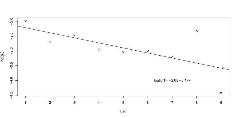
Figure 1: Sample autocorrelation coefficients and estimated regression line of $\log(\rho_{Y}(k))=\log(c)+k\cdot\log(\alpha)$.

By means of the estimation method described in Section Estimation, it can be seen that the estimated model for the hidden process is $X_{t}=0.109\cdot X_{t-1}+\epsilon_{t}$, being the observed process $Y_{t}$,

$$Y_{t}=\begin{cases}X_{t}&\text{with probability }0.240\\ 0.242\cdot X_{t}&\text{with probability }0.760\end{cases}$$ (5)

The estimated parameters are reported in Table 2.

Table 2: Bootstrap means and standard errors of the proposed model for the HPV example.

Parameter	Bootstrap mean	Bootstrap SE
$\hat{\mu_{\epsilon}}$	0.560	0.079
$\hat{\alpha}$	0.109	0.044
$\hat{\omega}$	0.760	0.154
$\hat{q}$	0.242	0.034

These results are highly consistent with those previously reported in the literature for the number of HPV cases obtained through a discrete time series approach [9] and can be interpreted in a very straightforward way. Moreover, this new methodology can be used to model the incidence of the disease instead of the number of cases, accounting for potential changes in the underlying population.

The estimated intensity of underreporting is $\hat{q}=0.242$, with 95% confidence interval $(0.176,0.308)$. The registered and estimated evolution of HPV incidence within the study period (2010-2014) can be seen in Figure 2.

These results indicate that only 34% of the HPV incidence in the considered period of time was actually recorded. Taking into account that public health cervical cancer prevention strategies are often designed on the basis of simulation models which are calibrated to registered HPV data [21], it is clear that providing decision makers with accurate data on HPV incidence is key to ensure optimal allocation of scarce public health funds.

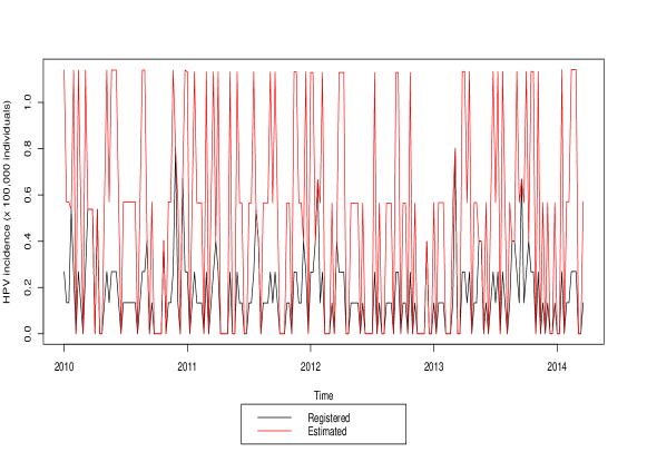
Figure 2: Registered and estimated HPV incidence in Girona in the period 2010-2014.

3.3 Example: COVID-19 incidence in the region of Heilongjiang

The betacoronavirus SARS-CoV-2 has been identified as the causative agent of an unprecedented world-wide outbreak of pneumonia starting in December 2019 in the city of Wuhan (China) [24], named as COVID-19. Considering that many cases run without developing symptoms beyond those of MERS-CoV, SARS-CoV or pneumonia due to other causes, it is reasonable to assume that the incidence of this disease has been underregistered, especially at the beginning of the outbreak [28]. This work focuses on the COVID-19 incidence registered in Heilongjiang province (north-eastern China) in the period (2020/01/22-2020/02/26), and it can be seen in Figure 3 that the registered data (black color) reflect only a fraction of the actual incidence (red color).

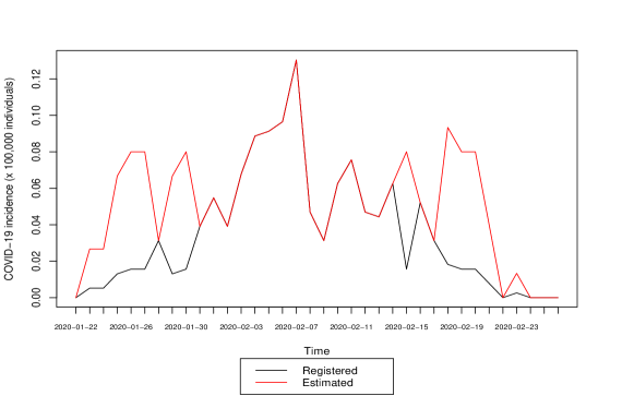
Figure 3: Registered (black) and estimated (red) COVID-19 incidence in the region of Heilongjiang in the period 2020/01/22-2020/02/26.

A disease with a similar behavior (MERS-CoV) has been modeled in a previous work as an $ARMA(3,1)$ [2], so we evaluated the performance of this model and similar ones. Probably due to the shortness of the available data this autoregressive structure was not observed and in our case the best performing model was an $MA(1)$ (AIC of -151.04 against -148.49 for the $ARMA(3,1)$), consistently with the residuals profile shown in Figure 4, obtained from fitting an $MA(1)$ model to the most likely process $X_{t}$ reconstructed following step (v) in Section Estimation.

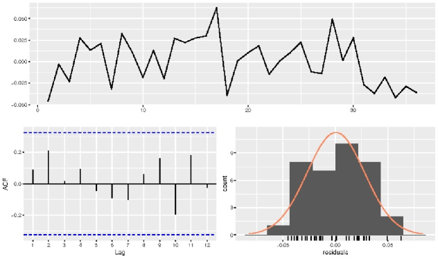
Figure 4: Residual analysis (raw residuals, ACF and histogram) from a $MA(1)$ model.

By means of the estimation method described in Section Estimation, it can be seen that the estimated model for the hidden process is $X_{t}=0.481\cdot\epsilon_{t-1}+\epsilon_{t}$, being the observed process $Y_{t}$,

$$Y_{t}=\begin{cases}X_{t}&\text{with probability }0.483\\ 0.194\cdot X_{t}&\text{with probability }0.517\end{cases}$$ (6)

The estimated parameters are reported in Table 3.

Table 3: Bootstrap means standard errors of the proposed model for the Covid-19 example.

Parameter	Bootstrap mean	Bootstrap SE
$\hat{\mu_{\epsilon}}$	0.057	0.014
$\hat{\theta}$	0.481	0.196
$\hat{\omega}$	0.517	0.180
$\hat{q}$	0.194	0.094

4 Discussion

In biomedical and epidemiological research, the usage of disease registries in order to analyse the impact and incidence of health issues is very common. However, the accuracy and data quality of such registries is in many cases at least doubtful. This is the case, for instance, for rare diseases [18] or health issues that clear asymptomatically in most cases like HPV infection. In the case of HPV incidence in Girona in the period 2010-2014, the registered weekly average is 0.17 cases per 100,000 individuals, while the reconstructed process has a weekly average of 0.50 cases per 100,000 individuals, showing that only 34% of the real incidence is recorded by the public health system. It must be considered that HPV infection is related to subsequent complications such as cervical cancer in some cases and that public health cervical cancer prevention strategies are often designed on the basis of simulation models which are calibrated to registered HPV data [21] and therefore the optimal allocation of scarce public health resources cannot be ensured if the under-reporting issue is not accounted for. This result is very consistent with that of [9], where the authors claim that only 38% of the HPV cases were registered in the same area and period of time.

The Heilongjiang region COVID-19 data reveal that in average about 66% of the actual incidence in the period 2020/01/22-2020/02/26 was reported. The unavailable data estimated by the proposed methodology are crucial to provide public health decision-makers with reliable information, which can also be used to improve the accuracy of dynamic models aimed to estimate the spread of the disease [28]. In China and almost globally afterwards, different non-pharmaceutical interventions were undertaken in order to minimise the impact of the disease on the general population and especially over the health systems, which were put to the limit of their capacity by the pandemic. In this context, one of the main challenges in predicting the evolution of the disease or evaluating the impact of these strategies is to use data as accurate as possible, taking into account that many COVID-19 cases are asymptomatic or with mild symptoms and a generalized shortage of testing kits [14], and therefore knowing that the registered number of affected individuals might be severely underestimated.

The concerns around accuracy of registered data have recently led to the publication of recommendations to improve data collection to ensure accuracy of registries (see for instance [19, 12]). Nonetheless, these recommendations are very recent and may be difficult for the public health services of many countries to fully implement them, due to operational or structural issues.

The proposed methodology is able to deal with underreported (or overreported) data in a very natural and straightforward way, estimating its intensity and frequency on a continuous time series, and allowing to reconstruct the most likely unobserved process. It is also flexible enough to handle covariates straightforwardly, and therefore it is simple to introduce trends or seasonality if necessary, so it can be useful in many contexts, where these issues might arise.

The simulation study shows that the proposed methodology behaves as expected and that the parameters used in the simulations, under different autocorrelation structures, are properly recovered, regardless of the intensity and frequency of the underreporting issues.

References

- [1] Jose H. Alfonso, Eva K. Løvseth, Yogindra Samant, and Jan-Ø. Holm. Work-related skin diseases in Norway may be underreported: data from 2000 to 2013. Contact Dermatitis, 72(6):409–412, jun 2015.
- [2] M. A. Alkhamis, A. Fernández-Fontelo, K. Vanderwaal, S. Abuhadida, P. Puig, and A. Alba-Casals. Temporal dynamics of Middle East respiratory syndrome coronavirus in the Arabian Peninsula, 2012-2017, 2019.
- [3] Susan Arendt, Lakshman Rajagopal, Catherine Strohbehn, Nathan Stokes, Janell Meyer, and Steven Mandernach. Reporting of foodborne illness by U.S. consumers and healthcare professionals. International journal of environmental research and public health, 10(8):3684–3714, 2013.
- [4] Amin Azmon, Christel Faes, and Niel Hens. On the estimation of the reproduction number based on misreported epidemic data. Statistics in medicine, 33(7):1176–92, mar 2014.
- [5] Tatiana Benaglia, Didier Chauveau, David R. Hunter, and Derek Young. mixtools : An R Package for Analyzing Finite Mixture Models. Journal of Statistical Software, 32(6):1–29, oct 2009.
- [6] Helen Bernard, Dirk Werber, and Michael Höhle. Estimating the under-reporting of norovirus illness in Germany utilizing enhanced awareness of diarrhoea during a large outbreak of Shiga toxin-producing E. coli O104: H4 in 2011 - a time series analysis. BMC Infectious Diseases, 14(1), mar 2014.
- [7] Peter J. Brockwell and Richard A. Davis. Time Series: Theory and Methods. chapter Stationary, pages 77–113. 1991.
- [8] Eileen F Dunne, Lauri E Markowitz, Mona Saraiya, Shannon Stokley, Amy Middleman, Elizabeth R Unger, Alcia Williams, and John Iskander. CDC grand rounds: Reducing the burden of HPV-associated cancer and disease. MMWR. Morbidity and mortality weekly report, 63(4):69–72, jan 2014.
- [9] Amanda Fernández-Fontelo, Alejandra Cabaña, Pedro Puig, and David Moriña. Under-reported data analysis with INAR-hidden Markov chains. Statistics in Medicine, 35(26):4875–4890, nov 2016.
- [10] Amanda Fernández‐Fontelo, Alejandra Cabaña, Harry Joe, Pedro Puig, and David Moriña. Untangling serially dependent underreported count data for gender‐based violence. Statistics in Medicine, 38(22):4404–4422, sep 2019.
- [11] Cheryl L Gibbons, Marie-Josée J Mangen, Dietrich Plass, Arie H Havelaar, Russell John Brooke, Piotr Kramarz, Karen L Peterson, Anke L Stuurman, Alessandro Cassini, Eric M Fèvre, Mirjam E E Kretzschmar, and Burden of Communicable diseases in Europe (BCoDE) consortium. Measuring underreporting and under-ascertainment in infectious disease datasets: a comparison of methods. BMC public health, 14(1):147, feb 2014.
- [12] Sonja Harkener, Jürgen Stausberg, Christiane Hagel, and Roman Siddiqui. Towards a Core Set of Indicators for Data Quality of Registries. Studies in health technology and informatics, 267:39–45, 2019.
- [13] Michael Höhle and Matthias an der Heiden. Bayesian nowcasting during the STEC O104:H4 outbreak in Germany, 2011. Biometrics, 70(4):993–1002, dec 2014.
- [14] Lei Huang, Xiuwen Zhang, Xinyue Zhang, Zhijian Wei, Lingli Zhang, Jingjing Xu, Peipei Liang, Yuanhong Xu, Chengyuan Zhang, Aman Xu, L Huang, and X Zhang. Rapid asymptomatic transmission of COVID-19 during the incubation period demonstrating strong infectivity in a cluster of youngsters aged 16-23 years outside Wuhan and characteristics of young patients with COVID-19: A prospective contact-tracing study. Journal of Infection, 80:e1–e13, 2020.
- [15] RJ Hyndman, G Athanasopoulos, C Bergmeir, G Caceres, L Chhay, M O’Hara-Wild, F Petropoulos, S Razbash, E Wang, and F Yasmeen. forecast: Forecasting functions for time series and linear models, 2018.
- [16] Rob J. Hyndman and Yeasmin Khandakar. Automatic time series forecasting: The forecast package for R. Journal of Statistical Software, 27(3):1–22, 2008.
- [17] Johannes Bracher. hhh4u: Fit an endemic-epidemic model to underreported data, 2019.
- [18] Yllka Kodra, Manuel Posada De La Paz, Alessio Coi, Michele Santoro, Fabrizio Bianchi, Faisal Ahmed, Yaffa R. Rubinstein, Jérôme Weinbach, and Domenica Taruscio. Data quality in rare diseases registries. In Advances in Experimental Medicine and Biology, volume 1031, pages 149–164. Springer New York LLC, 2017.
- [19] Yllka Kodra, Jérôme Weinbach, Manuel Posada-De-La-Paz, Alessio Coi, S. Lydie Lemonnier, David van Enckevort, Marco Roos, Annika Jacobsen, Ronald Cornet, S. Faisal Ahmed, Virginie Bros-Facer, Veronica Popa, Marieke van Meel, Daniel Renault, Rainald von Gizycki, Michele Santoro, Paul Landais, Paola Torreri, Claudio Carta, Deborah Mascalzoni, Sabina Gainotti, Estrella Lopez, Anna Ambrosini, Heimo Müller, Robert Reis, Fabrizio Bianchi, Yaffa R. Rubinstein, Hanns Lochmüller, and Domenica Taruscio. Recommendations for improving the quality of rare disease registries, aug 2018.
- [20] Pierre Magal and Glenn Webb. The parameter identification problem for SIR epidemic models: identifying unreported cases. Journal of Mathematical Biology, 77(6-7):1629–1648, dec 2018.
- [21] David Moriña, Silvia De Sanjosé, and Mireia DIaz. Impact of model calibration on cost-effectiveness analysis of cervical cancer prevention. Scientific Reports, 7(1):17208, dec 2017.
- [22] R Core Team. R: A Language and Environment for Statistical Computing, 2019.
- [23] Kenneth D. Rosenman, Alice Kalush, Mary Jo Reilly, Joseph C. Gardiner, Mathew Reeves, and Zhewui Luo. How much work-related injury and illness is missed by the current national surveillance system? Journal of Occupational and Environmental Medicine, 48(4):357–365, 2006.
- [24] Catrin Sohrabi, Zaid Alsafi, Niamh O’Neill, Mehdi Khan, Ahmed Kerwan, Ahmed Al-Jabir, Christos Iosifidis, and Riaz Agha. World Health Organization declares Global Emergency: A review of the 2019 Novel Coronavirus (COVID-19). International journal of surgery (London, England), feb 2020.
- [25] Theresa Stocks, Tom Britton, and Michael Höhle. Model selection and parameter estimation for dynamic epidemic models via iterated filtering: application to rotavirus in Germany. Biostatistics, sep 2018.
- [26] Oliver Stoner, Theo Economou, and Gabriela Drummond Marques da Silva. A Hierarchical Framework for Correcting Under-Reporting in Count Data. Journal of the American Statistical Association, pages 1–17, mar 2019.
- [27] Rainer Winkelmann. Markov Chain Monte Carlo analysis of underreported count data with an application to worker absenteeism. Empirical Economics, 21(4):575–587, 1996.
- [28] Zhao, Musa, Lin, Ran, Yang, Wang, Lou, Yang, Gao, He, and Wang. Estimating the Unreported Number of Novel Coronavirus (2019-nCoV) Cases in China in the First Half of January 2020: A Data-Driven Modelling Analysis of the Early Outbreak. Journal of Clinical Medicine, 9(2):388, feb 2020.