Bivariate $q$-normal distribution for transition strengths distribution from many-particle random matrix ensembles generated by $k$-body interactions

Abstract

Recently it is established, via lower order moments, that the univariate q-normal distribution, which is the weight function for $q$-Hermite polynomials, describes the ensemble averaged eigenvalue density from many-particle random matrix ensembles generated by $k$-body interactions [Manan Vyas and V.K.B. Kota, J. Stat. Mech. 2019, 103103 (2019)]. These ensembles are generically called embedded ensembles of $k$-body interactions [EE($k$)] and their GOE and GUE versions are called EGOE($k$) and EGUE($k$) respectively. Going beyond this work, the lower order bivariate reduced moments of the transition strength densities, generated by EGOE($k$) [or EGUE($k$)] for the Hamiltonian and an independent EGOE($t$) for the transition operator ${\cal O}$ that is $t$-body, are used to establish that the ensemble averaged bivariate transition densities follow the bivariate $q$-normal distribution. Presented are also formulas for the bivariate correlation coefficient $\rho$ and the $q$ values as a function of the particle number $m$, number of single particle states $N$ that the particles are occupying and the body ranks $k$ and $t$ of $H$ and ${\cal O}$ respectively. Finally, using the bivariate $q$ normal form a formula for the chaos measure number of principal components (NPC) in the transition strengths from a state with energy $E$ is presented.

I Introduction

Statistical properties of isolated finite many-particle systems such as atomic nuclei, mesoscopic systems (quantum dots, small metallic grains), interacting spin systems modeling quantum computing core, ultra-cold atoms, quantum black holes using SYK model and so on are being investigated with renewed interest in recent years for deeper understanding of quantum many-body chaos and thermalization in finite quantum systems. It is now well established that Random matrix theory is appropriate for providing answers to many of the questions in this topic. See Refs. kota ; zel-lea ; Rigol ; Verb-1 ; Verb-2 and references therein. In most of the finite many-particle quantum systems, their constituents predominantly interact via few-particle interactions. Therefore, modification of the classical Gaussian orthogonal (GOE) or unitary (GUE) or symplectic (GSE) random matrix ensembles with various deformations, incorporating information about interactions is essential. An appropriate model is to consider $m$ particles (in the present paper we will restrict to fermions) occupying $N$ single particle (sp) states and interacting with a $k$-body ($k<m$) interaction. In this situation, using a GOE/GUE/GSE representation for the Hamiltonian in $k$ particle spaces (defining random $k$-body interactions) and then propagating the information in the interaction to many particle spaces, we have embedded ensembles of $k$ particle interactions [EE($k$)] in $m$-particle spaces. Note that in these ensembles, a GOE/GUE/GSE random matrix ensemble in $k$-particle spaces is embedded in the $m$-particle $H$ matrix. Then, with GOE embedding, we have embedded Gaussian orthogonal ensemble of $k$-body interactions [EGOE($k$)] and similarly with GUE embedding EGUE($k$) kota . The two-body ensembles are first introduced in Fr-71 ; Bo-71 with reference to nuclear shell model and the seminal paper of Mon and French MF gave first analytical results for the general EGOE($k$). These early papers gave the remarkable result that as $k$ changes from 1 to $m$, EGOE($k$) [similarly EGUE($k$)] generates Gaussian to semi-circle transition in the eigenvalue density Br-81 . A more modern discussion of this results is due to Weidenmüller BW .

Most recently, Verbaarschot and collaborators extended the EGOE concept to the so called SYK model and pointed out that the weight function (giving orthogonal property) for $q$-Hermite polynomials describes the Gaussian to semi-circle transition in the eigenvalue density giving a functional for this transition Verb-1 . This weight function is called $q$-normal distribution in Sza-1 and throughout this paper we will use this name and its explicit form is given in Section 2. Using these observations combined with the asymptotic formulas for the lower order moments of the eigenvalue density generated by EGOE($k$) and EGUE($k)$ (both for fermion and boson systems), it is shown in a previous paper MaKo-19 that the $q$-normal distribution indeed gives the eigenvalue density for any $k$ in these ensembles and used here are the lower order moments of $q$-normal given in Ism-87 . In MaKo-19 , derived are also formulas for the parameter $q$ as a function of $(m,N,k)$. This result is also found to extend to the strength functions (also called local density of states).

Going beyond the eigenvalue densities, most important quantities in spectroscopy are transition strengths generated by a transition operator ${\cal O}$. Given an eigenstate $\left|E_{i}\right\rangle$ of $H$ in a $m$ particle space, action of ${\cal O}$ on this state will result in the transition to states $\left|E_{f}\right\rangle$ with transition probability or transition strength $\left|\left\langle E_{f}\mid{\cal O}\mid E_{i}\right\rangle\right|^{2}$. Multiplying this with the eigenvalue densities at $E_{i}$ and $E_{f}$ will give transition strength densities $\rho_{biv-{\cal O}}(E_{i},E_{f})$. In the situation that ${\cal O}$ a $t$-body operator, representing $H$ and ${\cal O}$ by independent EGOE($k$) and EGOE($t$), it was shown via the lower order moments of $\rho_{biv-{\cal O}}(E_{i},E_{f})$ that it will take bivariate Gaussian form for $(k,t)<<m$ (also assuming the dilute limit with $m\rightarrow\infty$, $N\rightarrow\infty$ and $m/N\rightarrow 0$) FKPT ; KoMa-15 . This result is used in several applications in nuclear structure, for example to calculate $\beta$-decay rates for pre-super novae stars, nuclear structure matrix elements for neutrinoless double beta decay and so on KM-94 ; KH-17 . An important unanswered question here is about the form of $\rho_{biv-{\cal O}}$ for all $k\leq m$ and $t\leq m$. The purpose of the present paper is to address this question and establish that indeed the form of $\rho_{biv-{\cal O}}$ in general will be bivariate $q$-normal distribution giving bivariate normal (Gaussian) form as $q\rightarrow 1$ and a bivariate semi-circle for $q=0$. Now we will give a preview.

In Section 2, we will introduce $q$-Hermite polynomials, $q$-normal distribution and also the bivariate $q$-normal distribution. Also presented here are some of their important properties. All the results in this Section are from Sza-1 ; Sza-2 . In Section 3, we will derive formulas the reduced bivariate moments $\mu_{rs}$, $r+s\leq 6$ of the bivariate $q$-normal distribution. Using these and the known results for EGOE and EGUE, in Section 4 established is the main result that the $\rho_{biv-{\cal O}}(E_{i},E_{f})$ follow bivariate $q$-normal form. Presented are also formulas for the bivariate correlation coefficient $\rho$ and the $q$ values, that define a bivariate $q$-normal, as a function of $(m,N,k,t)$. In Section 5, as an application of the bivariate $q$-normal, a formula in terms of an integral is given for the chaos measure number of principle components (NPC) in the transition strengths originating from a initial eigenstate of a $m$ particle Hamiltonian. Finally, Section 6 gives conclusions.

II $q$-Hermite polynomials and bivariate $q$-normal distribution

Let us begin with $q$-numbers $\left[n\right]_{q}$, $q$ factorials $\left[n\right]_{q}!$ and $q$-binomials $\left[\begin{smallmatrix}n\\ k\end{smallmatrix}\right]_{q}$,

$$\begin{array}[]{l}\left[n\right]_{q}=\displaystyle\frac{1-q^{n}}{1-q}=1+q+q^{2}+\ldots+q^{n-1}\;;\;\;\left[0\right]_{q}=0\;,\\ \left[n\right]_{q}!=\displaystyle\prod_{j=1}^{n}\left[j\right]_{q}!\;;\;\;\left[0\right]_{q}!=1\;,\\ \left[\begin{smallmatrix}n\\ k\end{smallmatrix}\right]_{q}=\displaystyle\frac{\left[n\right]_{q}!}{\left[n-k\right]_{q}!\;\left[k\right]_{q}!}\;;\;\;n\geq k\geq 0\;.\end{array}$$ (1)

Note that $\left[n\right]_{q=1}=n$, $\left[n\right]_{q=1}!=n!$ and $\left[\begin{smallmatrix}n\\ k\end{smallmatrix}\right]_{q=1}={n\choose k}$. Although we can use $-1\leq q\leq+1$, in the applications in this paper $0\leq q\leq 1$. With the $q$ numbers, the $q$-Hermite polynomials are defined by the relation

$$H_{n+1}(x|q)=xH_{n}(x|q)-\left[n\right]_{q}H_{n-1}(x|q)\;\;\mbox{with}\;\;n\geq 1,\;\;H_{-1}(x|q)=0,\;\;H_{0}(x|q)=1\;.$$ (2)

Note that $H_{n}(x|1)=H_{n}(x)$, the Hermite polynomials with respect to $1/\sqrt{2\pi}\,\exp-x^{2}/2$. Also, $H_{n}(x|0)=U_{n}(x/2)$, the Chebyshev polynomials that satisfy the relation

$$2xU_{n}(x)=U_{n+1}(x)+U_{n-1}(x)\;;\;\;\;U_{-1}(x)=0,\;U_{0}(x)=1\;.$$

Now, let us introduce the $q$-normal distribution $f_{qN}(x|q)$,

$$f_{qN}(x|q)=\displaystyle\frac{\displaystyle\sqrt{1-q}\displaystyle\prod_{\kappa=0}^{\infty}\left(1-q^{\kappa+1}\right)}{2\pi\,\displaystyle\sqrt{4-(1-q)x^{2}}}\;\displaystyle\prod_{k=0}^{\infty}\left[(1+q^{k})^{2}-(1-q)q^{k}x^{2}\right]\;.$$ (3)

The $f_{qN}(x|q)$ is defined over $S(q)$ with

$$S(q)=\left(-\displaystyle\frac{2}{\displaystyle\sqrt{1-q}}\;,\;+\displaystyle\frac{2}{\displaystyle\sqrt{1-q}}\right)$$

and $q$ in this work takes values $0$ to $1$. For $q=1$ taking the limit properly will give $S(q)=(-\infty,\infty)$. Note that the integral of $f_{qN}(x|q)$ over $S(q)$ is unity. It is easy to see that $f_{qN}(x|1)=1/\sqrt{2\pi}\,\exp-x^{2}/2$, the Gaussian and $f_{qN}(x|0)=(1/2\pi)\sqrt{4-x^{2}}$, the semi-circle. A very important property of $f_{qN}(x|q)$ is that it is the weight function with respect to which the $q$-Hermite polynomials are orthogonal over $S(q)$ giving,

$$\int_{S(q)}H_{n}(x|q)H_{m}(x|q)f_{qN}(x|q)dx=\left[n\right]_{q}!\;\delta_{mn}\;.$$ (4)

Going further, bivariate $q$-normal distribution $f_{biv-qN}(x,y|\rho,q)$ as given in Sza-1 is defined as follows,

$$\begin{array}[]{l}f_{biv-qN}(x,y|\rho,q)=f_{qN}(x|q)f_{qN}(y|q)h(x,y|\rho,q)\;;\\ h(x,y|\rho,q)=\displaystyle\prod_{k=0}^{\infty}\displaystyle\frac{1-\rho^{2}q^{k}}{(1-\rho^{2}q^{2k})^{2}-(1-q)\,\rho\,q^{k}\,(1+\rho^{2}q^{2k})\,xy+(1-q)\rho^{2}q^{2k}(x^{2}+y^{2})}\;,\end{array}$$ (5)

where $\rho$ is the bivariate correlation coefficient. The conditional $q$-normal densities ($f_{CqN}$) are then,

$$\begin{array}[]{l}f_{biv-qN}(x,y|\rho,q)=f_{qN}(x|q)f_{CqN}(y|x;\rho,q)=f_{qN}(y|q)f_{CqN}(x|y;\rho,q)\;;\\ f_{CqN}(x|y;\rho,q)=f_{qN}(x|q)h(x,y|\rho,q)\;,\\ f_{CqN}(y|x;\rho,q)=f_{qN}(y|q)h(x,y|\rho,q)\;.\end{array}$$ (6)

A very important property of $f_{CqN}$ is

$$\int_{S(q)}H_{n}(x|q)f_{CqN}(x|y;\rho,q)dx=\rho^{n}H_{n}(y|q)\;.$$ (7)

Putting $n=0$ in Eq. (7), it is easy to infer that $f_{CqN}$ and hence $f_{biv-qN}$ are normalized to unity over $S(q)$. We will make use of Eqs. (4) and (7) in the next Section to arrive at the main result of this paper given in Section 4. Let us mention that for $q=1$ and $0$, $f_{CqN}$ reduces to

$$\begin{array}[]{l}f_{CqN}(x|y;\rho,q=1)=\displaystyle\frac{1}{2\pi(\displaystyle\sqrt{1-\rho^{2}})}\,\exp-\displaystyle\frac{(x-\rho y)^{2}}{2(1-\rho^{2})}\;,\\ f_{CqN}(x|y;\rho,q=0)=\displaystyle\frac{(1-\rho^{2})\displaystyle\sqrt{4-x^{2}}}{2\pi\left[(1-\rho^{2})^{2}-\rho(1+\rho^{2})xy+\rho^{2}(x^{2}+y^{2})\right]}\;.\end{array}$$ (8)

There are many other properties of $q$-Hermite polynomials and $f_{CqN}$ as given in detail in Sza-1 ; Sza-2 . Some of these are,

$$\begin{array}[]{l}f_{biv-qN}(x,y|\rho,q)=f_{qN}(x|q)f_{qN}(y|q)\displaystyle\sum_{n=0}^{\infty}\displaystyle\frac{\rho^{n}}{\left[n\right]!}H_{n}(x|q)H_{n}(y|q)\;,\\ \phi(x,t|q)=\displaystyle\prod_{k=0}^{\infty}\left(1-(1-q)xtq^{k}+(1-q)t^{2}q^{2k}\right)^{-1}=\displaystyle\sum_{j=0}^{\infty}\displaystyle\frac{t^{j}}{\left[j\right]_{q}!}\,H_{j}(x|q)\;,\\ \displaystyle\int_{S(q)}P_{n}(x|y,\rho,q)P_{m}(x|y,\rho,q)f_{CqN}(x|y;\rho,q)dx=\left(\rho^{2}\right)_{n}\left[n\right]_{q}!\,\delta_{mn}\;.\end{array}$$ (9)

The first equality here can be used for example to obtain Eq. (7). The Second equality gives the generating $\phi(x,t|q)$ of the $q$-Hermite polynomials. In the third equality, $P_{n}(x|y,\rho,q)$ are Al-Salam-Chihara polynomials and $(\rho^{2})_{n}=\displaystyle\prod_{i=0}^{n-1}(1-\rho^{2}q^{i})$ with $(\rho^{2})_{0}=1$. Now, we will derive formulas for the reduced bivariate moments $\mu_{rs}$ of $f_{biv-qN}$.

III Reduced bivariate moments $\mu_{r+s}$, $r+s\leq 6$ of bivariate $q$-normal

Reduced bivariate central moments $\mu_{rs}$ of $f_{biv-qN}$ are defined by

$$\mu_{rs}=\displaystyle\int_{S(q)}x^{r}\,y^{s}\,f_{biv-qN}(x,y|\rho,q)\,dxdy\;.$$ (10)

As $H_{0}(x|q)=1$, $x=H_{1}(x|q)$ and $x^{2}=H_{2}(x|q)+1$, using Eqs. (4) and (7) will immediately give (note that the integrals of $f_{qN}$ and $f_{biv-qN}$ are 1) the results $\mu_{10}=\mu_{01}=0$ and $\mu_{20}=\mu_{02}=1$. Also $\mu_{rs}=\mu_{sr}$ and $\mu_{rs}=0$ for $r+s$ odd. As lower order moments suffice to arrive at the ensemble averaged forms of $\rho_{biv-{\cal O}}$, here we will consider only $\mu_{rs}$ of $f_{biv-qN}$ with $r+s=4$ and $6$ and $r\geq s$. To derive the formulas for $\mu_{rs}$, we will first write $x^{p}$, $p\leq 6$ in terms of $H_{n}(x|q)$, $n\leq 6$ using Eq. (2). This will give, after some algebra the formulas,

$$\begin{array}[]{rcl}x&=&H_{1}\;,\;\;\;x^{2}=H_{2}+H_{0}\;,\\ x^{3}&=&H_{3}+(2+q)H_{1}\;,\\ x^{4}&=&H_{4}+(3+2q+q^{2})H_{2}+(2+q)H_{0}\;,\\ x^{5}&=&H_{5}+(4+3q+2q^{2}+q^{3})H_{3}+(5+6q+3q^{2}+q^{3})H_{1}\;,\\ x^{6}&=&H_{6}+(5+4q+3q^{2}+2q^{3}+q^{4})H_{4}\\ &&+(9+13q+12q^{2}+7q^{3}+3q^{4}+q^{5})H_{2}+(5+6q+3q^{2}+q^{3})H_{0}\;.\end{array}$$ (11)

Here, $H_{n}$ stands for $H_{n}(x|q)$ and $H_{0}(x|q)=1$. Firstly, it is easy to see that $\mu_{11}=\rho$,

$$\begin{array}[]{rcl}\mu_{11}&=&\displaystyle\int_{S(q)}x\,y\,f_{biv-qN}(x,y|\rho,q)\,dxdy=\displaystyle\int_{S(q)}xf_{qN}(x|q)dx\displaystyle\int_{S(q)}H_{1}(y)f_{CqN}(y|x;\rho,q)dy\\ &=&\rho\;\displaystyle\int_{S(q)}H_{1}(x)H_{1}(x)f_{qN}(x|q)dx=\rho\;.\end{array}$$ (12)

In the first step here we have used Eqs. (11) and (7) and in the second step Eq. (4). For $r+s=4$ we need $\mu_{40}$, $\mu_{31}$ and $\mu_{22}$. The $\mu_{40}$ is simple,

$$\mu_{40}=\displaystyle\int_{S(q)}x^{4}f_{N}(x|q)dx=(2+q)\displaystyle\int_{S(q)}f_{N}(x|q)dx=(2+q)\;.$$ (13)

In the above we have substituted for $x^{4}$ the expansion in terms of $H_{n}$ using Eq. (11) and then used Eq. (4). Similarly, formula for $\mu_{31}$ is,

$$\begin{array}[]{rcl}\mu_{31}&=&\displaystyle\int_{S(q)}x^{3}\,y\,f_{biv-qN}(x,y|\rho,q)\,dxdy=\displaystyle\int_{S(q)}x^{3}f_{qN}(x|q)dx\displaystyle\int_{S(q)}H_{1}(y)f_{CqN}(y|x;\rho,q)dy\\ &=&\rho\;\displaystyle\int_{S(q)}\left[H_{3}(x|q)H_{1}(x|q)+(2+q)H_{1}(x|q)H_{1}(x|q)\right]f_{qN}(x|q)dx=\rho(2+q)=\rho\mu_{40}\;.\end{array}$$ (14)

Finally, proceeding to $\mu_{22}$ we have,

$$\begin{array}[]{rcl}\mu_{22}&=&\displaystyle\int_{S(q)}x^{2}\,y^{2}\,f_{biv-qN}(x,y|\rho,q)\,dxdy=\displaystyle\int_{S(q)}x^{2}f_{qN}(x|q)dx\displaystyle\int_{S(q)}\left[H_{2}(y|q)+1\right]f_{CqN}(y|x;\rho,q)dy\\ &=&\displaystyle\int_{S(q)}\left[H_{2}(x|q)+1\right]\left[\rho^{2}H_{2}(x|q)+1\right]f_{qN}(x|q)dx=1+(1+q)\rho^{2}\;.\end{array}$$ (15)

Turning to the sixth order moments first we have easily using $x^{6}$ and $x^{5}$ from Eq. (11),

$$\mu_{60}=(5+6q+3q^{2}+q^{3})\;,\;\;\;\mu_{51}=\rho\mu_{60}\;.$$ (16)

Formula for $\mu_{42}$ is,

$$\begin{array}[]{rcl}\mu_{42}&=&\displaystyle\int_{S(q)}x^{4}\,y^{2}\,f_{biv-qN}(x,y|\rho,q)\,dxdy\\ &=&\displaystyle\int_{S(q)}x^{4}f_{qN}(x|q)dx\displaystyle\int_{S(q)}\left[H_{2}(y|q)+1\right]f_{CqN}(y|x;\rho,q)dy\\ &=&\displaystyle\int_{S(q)}\left[H_{4}(x|q)+(3+2q+q^{2})H_{2}(x|q)+(2+q)\right]\left[\rho^{2}H_{2}(x|q)+1\right]f_{qN}(x|q)dx\\ &=&\rho^{2}(3+2q+q^{2})\left[2\right]_{q}!+(2+q)=(2+q)+\rho^{2}(3+5q+3q^{2}+q^{3})\;.\end{array}$$ (17)

Finally, $\mu_{33}$ is given by

$$\begin{array}[]{rcl}\mu_{33}&=&\displaystyle\int_{S(q)}x^{3}\,y^{3}\,f_{biv-qN}(x,y|\rho,q)\,dxdy\\ &=&\displaystyle\int_{S(q)}x^{3}f_{qN}(x|q)dx\displaystyle\int_{S(q)}\left[H_{3}(y|q)+(2+q)H_{1}(y|q)\right]f_{CqN}(y|x;\rho,q)dy\\ &=&\displaystyle\int_{S(q)}\left[H_{3}(x|q)+(2+q)H_{1}(x|q)\right]\left[\rho^{3}H_{3}(x|q)+\rho(2+q)H_{1}(x|q)\right]f_{qN}(x|q)dx\\ &=&(2+q)^{2}\rho+(1+q)(1+q+q^{2})\rho^{3}\;.\end{array}$$ (18)

Formulas for the bivariate moments given in Eqs. (13) - (18) can be derived also from the formulation presented in Sza-3 . Now, we will consider the bivariate moments of the transition strength densities generated by EGOE (and EGUE) and establish that the strength densities follow $f_{biv-qN}$ form.

Table 1: Reduced bivariate moments $\mu_{rs}$ from EGOE for a system of $m=10$ fermions with $k=2-6$ and $t=1$ and $2$. The results follow from Eqs. (20)-(23). Given also are values of the bivariate correlation coefficient $\rho$ and the $q$ values. Numbers in the brackets give the difference between EGOE values and those from the bivariate $q$-normal. Note that, for $k=6$ or higher the corrections to the $\mu_{rs}$ are $0$ and therefore the results for $k\geq 7$ are not shown in the table.

$k=2,t=1$	$k=2,t=2$
$\rho=0.8$,$\;\;q=0.622$	$\rho=0.622$,$\;\;q=0.622$
$\mu_{22}=2.013+(-0.025)$,$\;\;\mu_{60}=10.102+(-0.034)$	$\mu_{22}=1.595+(-0.034)$, $\;\;\mu_{60}=10.102+(-0.034)$
$\mu_{42}=7.095+(-0.336)$, $\;\;\mu_{33}=7.042+(-0.128)$	$\mu_{42}=5.246+(-0.285)$, $\;\;\mu_{33}=4.943+(-0.12)$
$k=3,t=1$	$k=3,t=2$
$\rho=0.7$,$\;\;q=0.292$	$\rho=0.467$,$\;\;q=0.292$
$\mu_{22}=1.607+(-0.026)$,$\;\;\mu_{60}=7.015+(-0.015)$	$\mu_{22}=1.257+(-0.025)$,$\;\;\mu_{60}=7.015+(-0.015)$
$\mu_{42}=4.47+(-0.144)$,$\;\;\mu_{33}=4.222+(-0.064)$	$\mu_{42}=3.213+(-0.111)$, $\;\;\mu_{33}=2.595+(-0.036)$
$k=4,t=1$	$k=4,t=2$
$\rho=0.6$,$\;\;q=0.071$	$\rho=0.333$,$\;\;q=0.071$
$\mu_{22}=1.374+(-0.011)$, $\;\;\mu_{60}=5.444+(0.0)$	$\mu_{22}=1.113+(-0.006)$,$\;\;\mu_{60}=5.444+(0.0)$
$\mu_{42}=3.248+(-0.038)$,$\;\;\mu_{33}=2.808+(-0.015)$	$\mu_{42}=2.426+(-0.021)$,$\;\;\mu_{33}=1.468+(-0.005)$
$k=5,t=1$	$k=5,t=2$
$\rho=0.5$,$\;\;q=0.004$	$\rho=0.222$,$\;\;q=0.004$
$\mu_{22}=1.25+(-0.001)$,$\;\;\mu_{60}=5.024+(0.0)$	$\mu_{22}=1.049+(0.0)$,$\;\;\mu_{60}=5.024+(0.0)$
$\mu_{42}=2.756+(-0.003)$, $\;\;\mu_{33}=2.133+(-0.001)$	$\mu_{42}=2.153+(-0.001)$,$\;\;\mu_{33}=0.903+(0.0)$
$k=6,t=1$	$k=6,t=2$
$\rho=0.4$,$\;\;q=0.0$	$\rho=0.133$,$\;\;q=0.0$
$\mu_{22}=1.16+(0.0)$,$\;\;\mu_{60}=5+(0.0)$	$\mu_{22}=1.018+(0.0)$, $\;\;\mu_{60}=5+(0.0)$
$\mu_{42}=2.48+(0.0)$, $\;\;\mu_{33}=1.664+(0.0)$	$\mu_{42}=2.053+(0.0)$, $\;\;\mu_{33}=0.536+(0.0)$

IV Bivariate $q$-normal representing bivariate transition strength densities generated by EGOE and EGUE

Let us say we have a system of $m$ fermions occupying $N$ number of sp states and the Hamiltonian ($H$) operator is $k$-body. Then, the $m$ particle space dimension is ${N\choose m}$. Starting with $H(k)$, it is possible to construct the $m$ particle $H$ matrix and obtain the eigenstates $\left|E\right\rangle$ with energy $E$ in $m$ particle spaces. Now, given a $t$-body transition operator ${\cal O}(t)$ acting on an eigenstate $\left|E_{i}\right\rangle$ in the $m$ particle space will populate the $m$ particle state $\left|E_{f}\right\rangle$ with probability $\left|\left\langle E_{f}\mid{\cal O}\mid E_{i}\right\rangle\right|^{2}$ and the resulting bivariate transition strength density (normalized to unity) is,

$$\rho_{biv-{\cal O}}(E_{i},E_{f})=\left[\left\langle\left\langle{\cal O}^{\dagger}{\cal O}\right\rangle\right\rangle^{m}\right]^{-1}\;\left\langle\left\langle{\cal O}^{\dagger}\delta(H-E_{f}){\cal O}\delta(H-E_{i})\right\rangle\right\rangle^{m}\;.$$ (19)

Note that $\left\langle\left\langle X\right\rangle\right\rangle^{m}=\sum_{E}\left\langle E\mid X\mid E\right\rangle$ where $\left|E\right\rangle$ are all the eigenstates of the $m$ particle Hamiltonian matrix. In order to derive the statistical law for the form of $\rho_{biv-{\cal O}}(E_{i},E_{f})$, random matrix theory is used by representing the $H$ by EGOE($k$) and the ${\cal O}$ by an independent EGOE($t$). With this, formulas for the (ensemble averaged) bivariate reduced central moments $\mu_{rs}$ of $\rho_{biv-{\cal O}}(E_{i},E_{f})$ are derived, as a function of $(m,k,t)$ using the so called binary correlation approximation for $r+s=4$ and $6$ (also for $\mu_{11}$); see Refs. FKPT ; Ko-01 . These results are also valid for the EGUE($k$) for $H$ and EGUE($t$) for ${\cal O}$; see kota . Further, for $\mu_{11}$ and $\mu_{rs}$ with $r+s=4$ results with finite $N$ corrections are derived in KoMa-15 . Quite strikingly, the formulas are close to those obtained for $f_{biv-qN}$. We will describe this in some detail below starting with the formulas without finite $N$ corrections.

IV.1 Equivalence between lower order moments

With EGOE($k$) for $H$ and EGOE($t$) for ${\cal O}$, the bivariate reduced central moments $\mu^{E}_{rs}$ for $r=s=1$ (the superscript $E$ denoting that the quantities are for the EGOE ensemble) and for $r+s=4$, using binary correlation approximation and the dilute limit conditions with $N\rightarrow\infty$ as described in FKPT ; Ko-01 ; MaKo-19 , are given by

$$\begin{array}[]{rcl}\mu^{E}_{11}&=&\displaystyle\frac{{m-t\choose k}}{{m\choose k}}\Rightarrow\rho^{E}=\displaystyle\frac{{m-t\choose k}}{{m\choose k}}\;,\\ \mu^{E}_{40}=\mu^{E}_{04}&=&2+\displaystyle\frac{{m-k\choose k}}{{m\choose k}}\Rightarrow q^{E}=\displaystyle\frac{{m-k\choose k}}{{m\choose k}}\;,\\ \mu^{E}_{31}=\mu^{E}_{13}&=&\rho^{E}\mu_{40}\;,\\ \mu^{E}_{22}&=&1+\left(\rho^{E}\right)^{2}(1+q^{E})+\rho^{E}\Delta_{0}\;;\\ \Delta_{0}&=&\displaystyle\frac{{m-k-t\choose k}}{{m\choose k}}-\displaystyle\frac{{m-t\choose k}{m-k\choose k}}{{m\choose k}^{2}}\;.\end{array}$$ (20)

Thus, $\mu_{11}$ gives the EGOE formula for the bivariate correlation coefficient $\rho^{E}$ and $\mu^{E}_{40}$ gives the formula for the $q^{E}$ parameter (see also MaKo-19 ). In terms of these, the formulas for $\mu^{E}_{31}$ and $\mu^{E}_{22}$ given in FKPT ; Ko-01 are rewritten in Eq. (20). To the extent that the correction $|\rho^{E}\Delta_{0}|\sim 0$, the $\mu^{E}_{rs}$ with $r+s=4$ from EGOE are same as the $\mu_{rs}$ from $f_{biv-qN}$. Numerical calculations using some typical values for $(m,k,t)$ show that this is indeed the situation; see Tables 1 and 2. Thus, the fourth order EGOE moments show that $f_{biv-qN}$ is a good representation of $\rho_{biv-{\cal O}}$. For further confirming this important result, we will turn to the sixth order bivariate moments.

Firstly, rewriting the formula for $\mu^{E}_{60}=\mu^{E}_{06}$ given in FKPT ; Ko-01 in terms of $q^{E}$ we have

$$\begin{array}[]{l}\mu^{E}_{60}=\mu^{E}_{06}=5+6q^{E}+3\left[q^{E}\right]^{2}+\left[q^{E}\right]^{3}+q^{E}\Delta_{1}\;;\;\;\Delta_{1}=\displaystyle\frac{{m-2k\choose k}}{{m\choose k}}-\left[\displaystyle\frac{{m-k\choose k}}{{m\choose k}}\right]^{2}\;,\\ \mu^{E}_{51}=\mu^{E}_{15}=\rho^{E}\,\mu^{E}_{60}\;.\end{array}$$ (21)

This is same as Eq. (16) provided the correction $\left|q^{E}\Delta_{1}\right|\sim 0$. Examples in Tables 1 and 2 confirm that this correction is indeed small. Using the expressions for $\Delta_{0}$ and $\Delta_{1}$ given in Eqs. (20) and (21), the formula for $\mu^{E}_{42}$ is

$$\begin{array}[]{l}\mu^{E}_{42}=\mu^{E}_{24}=(2+q^{E})+3\left[\rho^{E}\right]^{2}+5\left[\rho^{E}\right]^{2}q^{E}+3\left[\rho^{E}q^{E}\right]^{2}+\left[\rho^{E}\right]^{2}\left[q^{E}\right]^{3}+\rho^{E}(X)\;;\\ X=\Delta_{0}\left[3+2q^{E}+\Delta_{1}+(q^{E})^{2}\right]+\rho^{E}q^{E}\Delta_{1}-\rho^{E}(q^{E})^{2}+Y\;,\\ Y=\displaystyle\sum_{\nu=k}^{2k}\displaystyle\frac{{m-2\nu\choose k}{m-t-k\choose\nu-k}{k\choose 2k-\nu}}{{m\choose k}^{2}}\;.\end{array}$$ (22)

Similarly, simplifying the formula for $\mu^{E}_{33}$ we have,

$$\begin{array}[]{l}\mu^{E}_{33}=\rho^{E}\left[4+4q^{E}+(q^{E})^{2}\right]+\left\{\rho^{E}\right\}^{3}\left[1+2q^{E}+2(q^{E})^{2}+(q^{E})^{3}\right]+\rho^{E}(Z)\;;\\ Z=2\Delta_{0}^{2}+4\rho^{E}q^{E}\Delta_{0}+2\rho^{E}\Delta_{0}+\Delta_{0}\left[(q^{E})^{2}\rho^{E}+q^{E}\Delta_{0}+\Delta_{2}\right]+\rho^{E}q^{E}(q^{E}\Delta_{0}+\Delta_{2})\;,\\ \Delta_{2}=\displaystyle\frac{{m-t-2k\choose k}}{{m\choose k}}-\displaystyle\frac{{m-k-t\choose k}}{{m\choose k}}\displaystyle\frac{{m-k\choose k}}{{m\choose k}}\;.\end{array}$$ (23)

The formulas for $\mu^{E}_{42}$ and $\mu^{E}_{33}$ will be same as those from $f_{biv-qN}$ to the extent that the corrections $\left|\rho^{E}X\right|\sim 0$ in Eq. (22) and $\left|\rho^{E}Z\right|\sim 0$ in Eq. (23). This is indeed the situation as shown using two examples in Tables 1 and 2.

Results in Tables 1 and 2 clearly establish that in general the corrections $\rho^{E}\Delta_{0}$, $q^{E}\Delta_{1}$, $\rho^{E}X$ and $\rho^{E}Z$ for $\mu_{22}$, $\mu_{60}$, $\mu_{42}$ and $\mu_{33}$, with formulas for these given in Eqs. (20), (21), (22) and (23) respectively, are indeed less than 2-3% (in a few cases they are $\sim 5$%). Therefore, we conclude that the transition strength density generated by EGOE (similarly, EGUE) is well represented by the bivariate $q$-normal distribution. Let us mention that it is well known in statistics Kendall and in random matrix theory Br-81 ; KH-10 that lower order moments generate the form of a probability distribution.

Table 2: Reduced bivariate moments $\mu_{rs}$ from EGOE for a system of $m=15$ fermions with $k=2-8$ and $t=1$ and $2$. The results follow from Eqs. (20)-(23). Given also are values of the bivariate correlation coefficient $\rho$ and the $q$ values. Numbers in the brackets give the difference between EGOE values and those from the bivariate $q$-normal. Note that, for $k=8$ or higher the corrections to the $\mu_{rs}$ are $0$ and therefore the results for $k\geq 9$ are not shown in the table.

$k=2,t=1$	$k=2,t=2$
$\rho=0.867$, $\;\;q=0.743$	$\rho=0.743$, $\;\;q=0.743$
$\mu_{22}=2.296+(-0.013)$, $\;\;\mu_{60}=11.502+(-0.021)$	$\mu_{22}=1.941+(-0.021)$, $\;\;\mu_{60}=11.502+(-0.021)$
$\mu_{42}=9.022+(-0.315)$, $\;\;\mu_{33}=9.034+(-0.09)$	$\mu_{42}=7.302+(-0.285)$, $\;\;\mu_{33}=7.118+(-0.11)$
$k=3,t=1$	$k=3,t=2$
$\rho=0.8$, $\;\;q=0.484$	$\rho=0.629$, $\;\;q=0.484$
$\mu_{22}=1.93+(-0.019)$, $\;\;\mu_{60}=8.692+(-0.024)$	$\mu_{22}=1.561+(-0.025)$, $\;\;\mu_{60}=8.692+(-0.024)$
$\mu_{42}=6.239+(-0.233)$, $\;\;\mu_{33}=6.157+(-0.082)$	$\mu_{42}=4.747+(-0.199)$, $\;\mu_{33}=4.434+(-0.076)$
$k=4,t=1$	$k=4,t=2$
$\rho=0.733$, $\;\;q=0.242$	$\rho=0.524$, $\;\;q=0.242$
$\mu_{22}=1.651+(-0.017)$, $\;\;\mu_{60}=6.632+(-0.008)$	$\mu_{22}=1.323+(-0.018)$, $\;\;\mu_{60}=6.632+(-0.008)$
$\mu_{42}=4.511+(-0.096)$, $\;\;\mu_{33}=4.281+(-0.041)$	$\mu_{42}=3.367+(-0.081)$, $\;\;\mu_{33}=2.836+(-0.029)$
$k=5,t=1$	$k=5,t=2$
$\rho=0.667$, $\;\;q=0.084$	$\rho=0.429$, $\;\;q=0.084$
$\mu_{22}=1.472+(-0.009)$, $\;\;\mu_{60}=5.525+(-0.001)$	$\mu_{22}=1.192+(-0.007)$, $\;\;\mu_{60}=5.525+(-0.001)$
$\mu_{42}=3.58+(-0.033)$, $\;\;\mu_{33}=3.231+(-0.014)$	$\mu_{42}=2.691+(-0.025)$, $\;\;\mu_{33}=1.947+(-0.007)$
$k=6,t=1$	$k=6,t=2$
$\rho=0.6$, $\;\;q=0.017$	$\rho=0.343$, $\;\;q=0.017$
$\mu_{22}=1.363+(-0.003)$, $\;\;\mu_{60}=5.102+(0.0)$	$\mu_{22}=1.118+(-0.002)$, $\;\;\mu_{60}=5.102+(0.0)$
$\mu_{42}=3.119+(-0.008)$, $\;\;\mu_{33}=2.661+(-0.003)$	$\mu_{42}=2.375+(-0.005)$, $\;\;\mu_{33}=1.435+(-0.001)$
$k=7,t=1$	$k=7,t=2$
$\rho=0.533$, $\;\;q=0.001$	$\rho=0.267$, $\;\;q=0.001$
$\mu_{22}=1.285+(0.0)$, $\;\;\mu_{60}=5.007+(0.0)$	$\mu_{22}=1.071+(0.0)$, $\;\;\mu_{60}=5.007+(0.0)$
$\mu_{42}=2.856+(-0.001)$, $\;\;\mu_{33}=2.288+(0.0)$	$\mu_{42}=2.215+(0.001)$, $\;\;\mu_{33}=1.087+(0.0)$
$k=8,t=1$	$k=8,t=2$
$\rho=0.467$, $\;\;q=0.0$	$\rho=0.2$, $\;\;q=0.0$
$\mu_{22}=1.218+(0.0)$, $\;\;\mu_{60}=5+(0.0)$	$\mu_{22}=1.04+(0.0)$, $\;\;\mu_{60}=5+(0.0)$
$\mu_{42}=2.653+(0.0)$, $\;\;\mu_{33}=1.968+(0.0)$	$\mu_{42}=2.12+(0.0)$, $\;\;\mu_{33}=0.808+(0.0)$

IV.2 Formulas for correlation coefficient $\rho^{E}$ and parameter $q^{E}$ with finite $N$ corrections

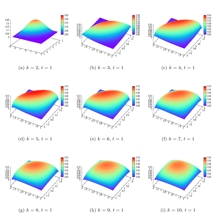
Figure 1: Bivariate transition strength density $f_{biv-qN}(x,y|\rho,q)$ given by Eq. (5) for $m=10$ fermions in $N=20$ sp levels using Eqs. (24) and (25) for the parameters $q$ and $\rho$ respectively. Parameters $k$ and $t$ are as indicated in the figure.

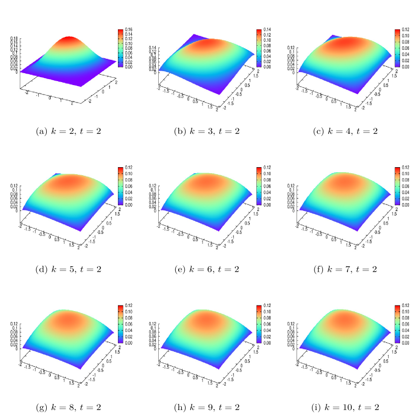
Figure 2: Bivariate transition strength density $f_{biv-qN}(x,y|\rho,q)$ given by Eq. (5) for $m=10$ fermions in $N=20$ sp levels using Eqs. (24) and (25) for the parameters $q$ and $\rho$ respectively. Parameters $k$ and $t$ are as indicated in the figure.

Although in the previous subsection we have used the dilute limit formulas (hence $N$, the number of sp states do not appear in the formulas), in applying the bivariate $q$-normal form for the transition strength densities, it is useful to have formulas for the two parameters $q^{E}$ and $\rho^{E}$ with finite $N$ corrections. As it is clearly established earlier in MaKo-19 , the EGOE and EGUE give essentially same numerical results for the lower order moments generating the same form the state densities (similarly for transition strength densities), we can use Eqs. (13) and (24) given in KoMa-15 , to write the formulas for $\rho^{E}$ and $q^{E}$ with finite $N$ corrections. For example, the formula for $q^{E}$ is, with EGUE($k$) [or EGOE($k$)] representing $H$,

$$\begin{array}[]{l}q^{E}=\displaystyle\binom{N}{m}^{-1}\displaystyle\sum_{\nu=0}^{min(k,m-k)}\;\displaystyle\frac{\Lambda^{\nu}(N,m,m-k)\;\Lambda^{\nu}(N,m,k)\;d(g_{\nu})}{\left[\Lambda^{0}(N,m,k)\right]^{2}}\;;\\ \\ \Lambda^{\nu}(N,m,r)=\displaystyle\binom{m-\nu}{r}\;\displaystyle\binom{N-m+r-\nu}{r}\;,\\ \\ d(g_{\nu})=\displaystyle\binom{N}{\nu}^{2}-\displaystyle\binom{N}{\nu-1}^{2}\;.\end{array}$$ (24)

Note that we are considering $m$ fermions in $N$ sp states with $H$ a $k$-body operator. Similarly, with ${\cal O}$ a $t$-body operator represented by an independent EGUE($t$) [or EGOE( $t$)], the bivariate correlation coefficient $\rho^{E}$ is given by,

$$\rho^{E}=\displaystyle\sum_{\nu=0}^{min(t,m-k)}\;\displaystyle\frac{\Lambda^{\nu}(N,m,m-t)\;\Lambda^{\nu}(N,m,k)\;d(g_{\nu})}{\binom{N}{m}\;\Lambda^{0}(N,m,k)\;\Lambda^{0}(N,m,t)}\,.$$ (25)

Although we have restricted to ${\cal O}(t)$ type operators in this paper, it is also possible to analyze $\mu^{E}_{rs}$ with $r+s=4$ and $(rs)=(11)$ for beta and neutrinoless double beta decay type operators and also for particle removal operators using the results in KoMa-15 . More importantly, they will give formulas, with finite $N$ corrections, for $\rho^{E}$ and $q^{E}$ for the transition strength densities generated by these operators.

Figure 1 shows the bivariate transition strength density $f_{biv-qN}(x,y|\rho,q)$ given by Eq. (5) for $m=10$ fermions in $N=20$ sp levels. Parameters $q$ and $\rho$ are calculated using Eqs. (24) and (25) respectively; see Table 3 for numerical values. Here, $t=1$ and $k$ varies from 2 to 10. As can be seen from this figure, the bivariate transition strength density is close to Gaussian form for small $k$ and becomes semi-circular like with increasing $k$. Similarly, Figure 2 shows the bivariate transition strength density $f_{biv-qN}(x,y|\rho,q)$ with $t=2$. The transition in $f_{biv-qN}(x,y|\rho,q)$ from Gaussian to semi-circular form is faster for $t=2$ in comparison to that for $t=1$.

Table 3: Correlation coefficient $\rho$ and parameter $q$ with finite-$N$ corrections. Values are given for a system of $m=10$ fermions in $N=20$ sp levels.

$t$	$k$	$\rho$	$q$	$t$	$k$	$\rho$	$q$
1	2	0.682	0.465	2	2	0.465	0.465
	3	0.559	0.176		3	0.314	0.176
	4	0.455	0.044		4	0.210	0.044
	5	0.364	0.007		5	0.136	0.007
	6	0.284	0.001		6	0.085	0.001
	7	0.214	0.000		7	0.050	0.000
	8	0.152	0.000		8	0.027	0.000
	9	0.096	0.000		9	0.012	0.000
	10	0.046	0.000		10	0.004	0.000

V Application of bivariate $q$-normal form of the strength densities

Using the bivariate $q$-normal form for the strength densities and using the formulation given in KS-PLB ; KGK-PRE , it is possible to derive formulas for the chaos measures number of principle components (NPC) and information entropy in transition strengths. For example, (NPC)_E in transition strengths generated by the action of a transition operator ${\cal O}(t)$ on an eigenstate with energy $E$ [of a given $(m,N)$ system with $k$-body interactions] gives the number of $m$-particle eigenstates excited by the transition operator. Note that, (NPC)_E is small implies that the state $E$ is collective or regular with respect to ${\cal O}$ and if it is large then the state is chaotic or mixed. Eq. (6) of KS-PLB gives,

$$(\mbox{NPC})_{E}=\displaystyle\frac{d}{3}\;\left[\rho_{1:{\cal O}}(E)\right]^{2}\;\left\{\displaystyle\int_{\epsilon_{0}^{i}}^{\epsilon_{0}^{f}}dE_{f}\;\displaystyle\frac{\left[\rho_{biv-{\cal O}}(E,E_{f})\right]^{2}}{\rho(E_{f})}\right\}^{-1}\;.$$ (26)

Here, $d=\binom{N}{m}$ is the dimension of the space, $\rho(E_{f})$ is the normalized state density of the final states with energy $E_{f}$, $\rho_{biv-{\cal O}}$ is the normalized bivariate transition strength density and $\rho_{1:{\cal O}}$ is the marginal density of $\rho_{biv-{\cal O}}$. We will give the values of $\epsilon_{0}^{i}$ and $\epsilon_{0}^{f}$ ahead. Putting the centroids and widths $(\epsilon_{1},\sigma_{1})$ and $(\epsilon_{2},\sigma_{2})$ of $E$ and $E_{f}$ respectively in $\rho_{biv-{\cal O}}$ and similarly the centroid and width $(\epsilon_{f},\sigma_{f})$ of $\rho(E_{f})$ we have from Sections II and IV,

$$\begin{array}[]{l}\rho(E_{f})=\displaystyle\frac{1}{\sigma_{f}}\;f_{qN}\left(\frac{E-\epsilon_{f}}{\sigma_{f}}\mid q^{\prime}\right)\\ \mbox{with}\;\;\epsilon_{f}-\displaystyle\frac{2\sigma_{f}}{\displaystyle\sqrt{1-q^{\prime}}}\leq E_{f}\leq\epsilon_{f}+\displaystyle\frac{2\sigma_{f}}{\displaystyle\sqrt{1-q^{\prime}}}\;,\\ \\ \rho_{biv-{\cal O}}(E,E_{f})=\displaystyle\frac{1}{\sigma_{1}\sigma_{2}}\;f_{biv-qN}\left(\hat{E},\frac{E_{f}-\epsilon_{2}}{\sigma_{2}}\mid\rho,q\right)\;;\;\hat{E}=(E-\epsilon_{1})/\sigma_{1}\\ \mbox{with}\;\;\epsilon_{2}-\displaystyle\frac{2\sigma_{2}}{\displaystyle\sqrt{1-q}}\leq E_{f}\leq\epsilon_{2}+\displaystyle\frac{2\sigma_{2}}{\displaystyle\sqrt{1-q}}\;\;\mbox{and}\;\;\epsilon_{1}-\displaystyle\frac{2\sigma_{1}}{\displaystyle\sqrt{1-q}}\leq E\leq\epsilon_{1}+\displaystyle\frac{2\sigma_{1}}{\displaystyle\sqrt{1-q}}\;,\\ \\ \rho_{1:{\cal O}}(E)=\displaystyle\frac{1}{\sigma_{1}}\;f_{qN}(\hat{E}|q)\;.\end{array}$$ (27)

Note that the $q$ value for $\rho_{biv-{\cal O}}(E,E_{f})$ and $\rho(E_{f})$ need not be same in general, i.e. $q\neq q^{\prime}$. Substituting all those in Eq. (27) in Eq. (26) will give the following formula,

$$\begin{array}[]{l}(\mbox{NPC})_{E}=\displaystyle\frac{d}{3}\;\left[f_{qN}(\hat{E}|q)\right]^{2}\;\left\{\displaystyle\int_{y_{0}^{i}}^{y_{0}^{f}}dy\;\hat{\sigma}\;\displaystyle\frac{\left[f_{biv-qN}(\hat{E},y|\rho,q)\right]^{2}}{f_{qN}\left(\frac{y-\hat{\Delta}}{\hat{\sigma}}\left|q^{\prime}\right.\right)}\right\}^{-1}\;;\\ \\ \hat{\sigma}=\displaystyle\frac{\sigma_{f}}{\sigma_{2}}\;,\;\;\;\hat{\Delta}=\displaystyle\frac{\epsilon_{f}-\epsilon_{2}}{\sigma_{2}}\;,\\ \\ y_{0}^{i}=max\left(\hat{\Delta}-\displaystyle\frac{2\hat{\sigma}}{\displaystyle\sqrt{1-q^{\prime}}}\;,\;-\displaystyle\frac{2}{\displaystyle\sqrt{1-q}}\right)\;,\;\;y_{0}^{f}=min\left(\hat{\Delta}+\displaystyle\frac{2\hat{\sigma}}{\displaystyle\sqrt{1-q^{\prime}}}\;,\;\displaystyle\frac{2}{\displaystyle\sqrt{1-q}}\right)\;.\end{array}$$ (28)

It is of interest in future to apply Eq. (28) to some realistic examples and also check in some examples if $\hat{\sigma}\sim 1$ and $\hat{\Delta}\sim 0$.

Figure 3 shows $(\mbox{NPC})_{E}$ given by Eq. (28) as a function of $E$ for various $k$ with $t=1$ (left panel) and $t=2$ (right panel). Results are shown for $m=10$ fermions in $N=20$ sp levels and the parameters $q$ and $\rho$ are obtained using Eqs. (24) and (25) respectively; see Table 3 for numerical values. We assume $\hat{\sigma}=1$, $\hat{\Delta}=0$ and $q=q^{\prime}$. Note that the $H$ matrix dimension for this system is $d=\binom{20}{10}=184756$. It is seen from the figure that for a given $t$, there is a transition from Gaussian form to the GOE result (GOE gives NPC to be $d/3\sim 61585$) with increasing $k$. This transition is faster for larger $t$.

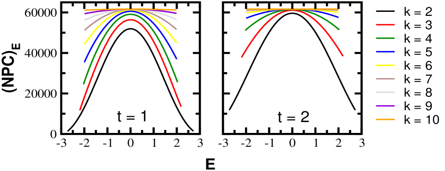
Figure 3: $(\mbox{NPC})_{E}$ given by Eq. (28) as a function of $E$ for various $k$ values with $t=1$ (left panel) and $t=2$ (right panel). Results are shown for $m=10$ fermions in $N=20$ sp levels and the parameters $q$ and $\rho$ are obtained using Eqs. (24) and (25) respectively. We assume $\hat{\sigma}=1$, $\hat{\Delta}=0$ and $q=q^{\prime}$. Note that $E$ in the figure is same as $\hat{E}$ in Eqs. (27) and (28).

VI Conclusions

Using lower order bivariate moments, it is established that the transition strength densities generated by EGOE and EGUE random matrix ensembles follow bivariate $q$-normal form. Formulas for the correlation coefficient $\rho^{E}$ and the parameter $q^{E}$ are also given as a function of $(N,m,k,t)$ for $m$ fermions in $N$ sp states with the Hamiltonian operator $H(k)$ and transition operator ${\cal O}(t)$ represented by independent EGUE($k$) and EGUE($t$) respectively. These formulas are expected to apply to EGOE and this follows from kota ; KoMa-15 ; MaKo-19 . In addition, application of the bivariate $q$-normal to the NPC in transition strengths is described by deriving a formula involving an integral.

Using $f_{biv-qN}$ and its extensions, it should be possible to address several important issues in the subject of embedded ensembles with $k$-body interactions [EE($k$)]. Some of these are as follows. (i) It is possible to study the measures for wavefunction structure, as given by the form of the strength functions $F_{k}(E)$, number of principal components (NPC)_E and information entropy $S^{info}(E)$ kota ; KS-01 , for a system of $m$ particles (fermions or bosons) in a one-body mean-field with $N$ sp states and interacting with a $k$-body force. Then, $H=h(1)+\lambda V(k)$ with $V(k)$ represented by EGOE($k)$ or EGUE($k$). This is under investigation ChvMan . Here, one complication compared to the $k=2$ analysis given in KS-01 is that the $V(k)$ with $k\geq 3$ will have more than two $U(N)$ tensorial parts with tensorial rank $\nu=1,2,\ldots,k$ ($\nu=0$ part is not important here). (ii) It may be possible to study the two-point function that gives the number variance (fluctuations) for EGOE and EGUE using $q$-Hermite polynomials and the results in Refs. Verb-2 ; LHKC . (iii) Although $f_{CqN}(x|y;\rho,q)$ gives $F_{k}(E)$ changing from Gaussian form to a semi-circle like form, this will not give the Breit-Wigner (BW) form for $F_{k}(E)$ in any limit (BW form appears for small values of $\lambda$). It is important to study $q$ extended $t$-distribution so that the BW form is also included; see kota for the role of $t$-distribution in describing strength functions. (iv) The bivariate $t$-distribution describes transition strength densities for $\lambda$ small in $H=h(1)+\lambda V(k)$ as shown in KCS-06 for $k=2$. Therefore, it is important to study its $q$ extensions. (v) With other quantum numbers such as $J$ for the eigenstates, trivariate $q$-normal and in general multivariate $q$-normal distributions may prove to be useful in random matrix theory with $k$-body interactions; see Sza-1 ; Sza-2 ; Sza-4 for some properties of tri- and multi-variate $q$-normal distributions. It is also of interest to investigate the usefulness of the modified $q$-normal $\phi(x,t|q)f_{qN}(x|q)$ discussed in Sza-1 .

- (1) V. K. B. Kota, Embedded Random Matrix Ensembles in Quantum Physics (Springer-Verlag, Heidelberg 2014).
- (2) F. Borgonovi, F. M. Izrailev, L. F. Santos, and V. G. Zelevinsky, Phys. Rep. 626, 1 (2016).
- (3) L. D’Alessio, Y. Kafri, A. Polkovnikov, and M. Rigol, Adv. Phys. 65, 239 (2016).
- (4) A. M. García-García and J. J. M. Verbaarschot, Phys. Rev. D 96, 066012 (2017).
- (5) Y. Jia and J. J. M. Verbaarschot, arXiv:1912.11923 [hep-th] (2019).
- (6) J. B. French and S. S. M. Wong, Phys. Lett. B33, 449 (1970).
- (7) O. Bohigas and J. Flores, Phys. Lett. B34, 261 (1971).
- (8) K. K. Mon and J.B. French, Ann. Phys. (N.Y.) 95, 90 (1975).
- (9) T. A. Brody, J. Flores, J. B. French, P. A. Mello, A. Pandey, and S. S. M. Wong, Rev. Mod. Phys. 53, 385 (1981).
- (10) L. Benet, T. Rupp, and H. A. Weidenmüller, Ann. Phys. (N.Y.) 292, 67 (2001).
- (11) P. J. Szablowski, Electronic Journal of Probability 15, 1296 (2010).
- (12) Manan Vyas and V.K.B. Kota, J. Stat. Mech. 2019, 103103 (2019).
- (13) M. E. H. Ismail, D. Stanton, and G. Viennot, Europ. J. Combinatorics 8, 379 (1987).
- (14) J.B. French, V.K.B. Kota, A. Pandey, and S. Tomsovic, Ann. Phys. (N.Y.) 181, 235 (1988).
- (15) V.K.B. Kota and Manan Vyas, Ann. Phys. (N.Y.) 359, 252 (2015).
- (16) V.K.B. Kota and D. Majumdar, Z. Phys. A351, 377 (1995).
- (17) V.K.B. Kota, AIP Conf. Proc. 1912, 020009 (2017).
- (18) P.J. Szablowski, Demonstratio Mathematica, 46, 679 (2013).
- (19) P.J. Szablowski, moments, arXiv:1506.07970 [math-PR] (2015).
- (20) V.K.B. Kota, Physics Reports 347, 223 (2001).
- (21) A. Stuart and J.K. Ord, Kendall’s Advanced Theory of Statistics : Distribution Theory (Oxford University Press, New York, 1987).
- (22) V.K.B. Kota and R.U. Haq, Spectral Distributions in Nuclei and Statistical Spectroscopy (World Scientific, Singapore, 2010).
- (23) V.K.B. Kota and R. Sahu, Phys. Lett. B429, 1 (1998).
- (24) J.M.G. Gómez, K. Kar, V.K.B. Kota, R.A. Molina, and J. Retamosa, Phys. Rev. C 69, 057302/1-4 (2004).
- (25) Priyanka Rao, Manan Vyas, and N.D. Chavda, in preparation (2020).
- (26) V.K.B. Kota and R. Sahu, Phys. Rev. E 64, 016219 (2001).
- (27) R.J. Leclair, R.U. Haq, V.K.B. Kota, and N.D. Chavda, Phys. Lett. A 372, 4373 (2008).
- (28) V.K.B. Kota, N.D. Chavda, and R. Sahu, Phys. Rev. E 73, 047203 (2006).
- (29) P.J. Szablowski, arXiv:1712.04250v5 [math-PR] (2019).