Identification of pre-biotic molecules containing Peptide-like bond in a hot molecular core, G10.47+0.03

Abstract

After hydrogen, oxygen, and carbon, nitrogen is one of the most chemically active species in the interstellar medium (ISM). Nitrogen bearing molecules have great importance as they are actively involved in the formation of biomolecules. Therefore, it is essential to look for nitrogen-bearing species in various astrophysical sources, specifically around high-mass star-forming regions where the evolutionary history is comparatively poorly understood. In this paper, we report observation of three potential pre-biotic molecules, namely, isocyanic acid (HNCO), formamide ($\rm{NH_{2}CHO}$), and methyl isocyanate ($\rm{CH_{3}NCO}$), which contain peptide-like bonds (-NH-C(=O)-) in a hot molecular core, G10.47+0.03 (hereafter, G10). Along with the identification of these three complex nitrogen-bearing species, we speculate their spatial distribution in the source and discuss their possible formation pathways under such conditions. Rotational diagram method under LTE condition has been employed to estimate the excitation temperature and the column density of the observed species. Markov Chain Monte Carlo method was used to obtain the best suited physical parameters of G10 as well as line properties of some species. We also determined the hydrogen column density and the optical depth for different continuum observed in various frequency ranges. Finally, based on these observational results, we have constructed a chemical model to explain the observational findings. We found that HNCO, $\rm{NH_{2}CHO}$, and $\rm{CH_{3}NCO}$ are chemically linked with each other.

Keywords: Astrochemistry - line: identification - ISM: individual (G10.47+0.03) - ISM: molecules, ISM: abundance.

1 Introduction

Various inter-disciplinary studies are involved in the search of the origin of life on Earth. Whether life evolved ab-initio here on the Earth or came from another part of the space is debatable, but it is accepted that our ancestors (may be the unicellular species) should have formed from the raw materials present at that time somewhere in the universe. When, where, and how the first life came is not straight forward to answer. However, at the current era, it is necessary to try to explain how the building blocks of life (simple $\rightarrow$ complex molecule $\rightarrow$ bio-molecule) could be indigenously produced in the universe.

Around $200$ molecular species have been identified in the ISM or circumstellar shells (https://www.astro.uni-koeln.de/cdms/molecules). Among them several species are marked as the precursor to biomolecules. Study of the pre-biotic molecules is always fascinating as they involved in the formation of amino acids, proteins, and the basic building blocks of life (Chakrabarti & Chakrabarti, 2000a, b; Das et al., 2008; Garrod, 2013; Chakrabarti et al., 2015; Majumdar et al., 2015; Das et al., 2019). Protein synthesis occurs through peptide bond formation (Goldman et al., 2010). CN is the first observed nitrogen-bearing species in space (McKellar, 1940). Since then, various nitrogen-bearing species were identified in numerous astronomical objects. Hot core regions are the unique laboratory of complex organic molecules (COMs). Forest of molecular lines has been identified in several hot molecular cores (HMCs) (e.g., Belloche et al., 2016; Garrod et al., 2017). Here, we will focus on the observation done towards a hot molecular core, G10, which is located at a distance of 8.6 kpc (Sanna et al., 2014) having luminosity $\rm{5\times 10^{5}\ L_{\odot}}$ (Cesaroni et al., 2010).

Among the pre-biotic molecules, methanimine (CH₂NH) and methylamine ($\rm{CH_{3}NH_{2}}$) are the simple imine and amine respectively which play a significant role in the synthesis of the simplest amino acid, glycine ($\rm{NH_{2}CH_{2}COOH}$) (Altwegg et al., 2017; Sil et al., 2018). These molecules have been identified in G10, which strengthens the possibility of the presence of glycine in this source (Ohishi et al., 2017).

Isocyanic acid (HNCO) is the simple molecule which has four biogenic elements (C, N, O, and H) making a peptide bond, -NH-C(=O)-. HNCO was observed long ago towards the high-mass star-forming region, Sgr B2 (Snyder & Buhl, 1972). Presently, it has been observed in various astronomical objects such as translucent molecular cloud (Turner et al., 1999), dense core (Marcelino et al., 2018), and low-mass protostar, IRAS 16293-2422 (Bisschop et al., 2008). It was also previously detected in G10 (Wyrowski et al., 1999).

Formamide (NH₂CHO) is the simplest possible amide and a potential pre-biotic molecule which contains a peptide bond that can link with the amino acids and form proteins. NH₂CHO is also a precursor of genetic and metabolic molecules (Saladino et al., 2012). This molecule is one of the key species for the formation of nucleobases and nucleobase analogs. NH₂CHO was observed for the first time towards high-mass star-forming region, Sgr B2 (Rubin et al., 1971). Subsequently, it was identified in other hot cores, such as, Orion KL, G327.3-0.6, G34-3+0.15, NGC 6334 (Turner, 1991; Bøgelund et al., 2019), solar-type low-mass protostar IRAS 16293-2422 (Kahane et al., 2013), and in the shock of the prestellar core, L1157-B1 (Codella et al., 2017). NH₂CHO was previously detected in G10 using millimeter and sub-millimeter wavelength facility with Sub-millimeter Array (SMA) observation (Rolffs et al., 2011).

Methyl isocyanate (CH₃NCO) is another potential pre-biotic molecules, which also has a peptide-like bond. It has recently been observed in a high-mass star-forming region, Sgr B2 (Cernicharo et al., 2016) and low-mass star-forming region, IRAS 16293-2422 (Ligterink et al., 2017; Martín-Doménech et al., 2017). Here, for the first time, we are reporting the identification of CH₃NCO in G10. HNCO has firmly been identified in G10, but for NH₂CHO, no clear peak was present in the observed spectra of Rolffs et al. (2011). Recently, HNCO and NH₂CHO both have been identified, but $\rm{CH_{3}NCO}$ has been tentatively identified in the 67P/Churyumov-Gerasimenko comet by Double Focusing Mass Spectrometer (DFMS) of the ROSINA experiment on ESA’s Rosetta mission (Altwegg et al., 2017).

In this paper, we present a combined study of observational analysis and chemical modeling of the peptide-like bond molecules. We report identifications of HNCO, $\rm{NH_{2}CHO}$, and $\rm{CH_{3}NCO}$ in G10. To understand the formation of these three species, we prepare a chemical model which mimics the observed results. We have organized this paper as follows. In Section 2, we describe observational details and data analysis procedures. Observational results are presented in Section 3. Chemical model and results are described in Section 4. Finally, in Section 5, we make concluding remarks.

2 Observations, data analysis and line identification

In this paper, we have used ALMA cycle 4 archival data of G10.47+0.03 observation ($\#$2016.1.00929.S.). The phase center of the observation is located at $\alpha$(J2000)=18^h08^m38.232^s and $\delta$(J2000)=-19⁰51^′50.4${}^{{}^{\prime\prime}}$. Observations were performed with ALMA Band 4 covering four spectral ranges; (i) 129.50-131.44 GHz, (ii) 147.50-149.43 GHz, (iii) 153.00-154.93 GHz, and (iv) 158.49-160.43 GHz. In this observation, the flux calibrator was J1733-1304, the phase calibrator was J1832-2039 and the bandpass calibrator was J1924-2914. The systematic velocity of this source was $67-68$ Km s^-1 (Rolffs et al., 2011). Observational summary is given in Table 1. All the analysis, such as spectral and line analysis, were done using CASA 4.7.2 software (McMullin et al., 2007). We have implemented a first-order baseline fit by using ‘uvcontsub’ command available in the CASA program. We have divided each spectral window into two data cubes: continuum and line emission for the analysis. We did not apply the self-calibration and ALMA missing flux correction. The line identification of all the observed species presented in this paper was carried out using CASSIS software together with the Cologne Database for Molecular Spectroscopy (CDMS, Müller et al., 2001, 2005) and Jet Propulsion Laboratory (JPL, Pickett et al., 1998). To firmly identify a molecular transition corresponding to the observed spectra, we checked line blending, V_LSR velocity, upper state energy (E_up), and Einstein coefficient. After assigning a molecular species to the observed spectral feature, we used LTE modeling to confirm or reject the identification.

Table 1: Summary of the observation.

Source name	Observation date	On-source time	Number	Frequency range	Channel spacing	Baseline
	yyyy-dd-mm	hh:mm	of antennas	GHz	kHz	Maximum (m)	Minimum (m)
G10.47+0.03	2017-05-03	001:53	39	129.50-131.44	244, 976	310	15
	2017-28-01	00:33.6	40	147.50-149.43	244, 976	272	15
	2017-06-03	01:03.5	41	153.00-154.93	244, 976	331	15
	2017-07-03	00:28.72	39	158.49-160.63	244, 976	331	15

3 Observational results

3.1 Continuum images

Cesaroni et al. (2010) observed G10 with a very large array (VLA) and identified three distinct HII regions A, B1, and B2 inside the HMC. The RMS noises of these observation were 269 $\mu$Jy/beam, $73$ $\mu$Jy/beam, 773 $\mu$Jy/beam, and 227 $\mu$Jy/beam for 6 cm, $3.6$ cm, 2 cm, and $1.3$ cm continuum and corresponding synthesized beam and position angle are 0${}^{{}^{\prime\prime}}$.73$\times$0${}^{{}^{\prime\prime}}$.42 and -11^∘.2; 0${}^{{}^{\prime\prime}}$.37$\times$0${}^{{}^{\prime\prime}}$.19 and -15^∘.5; 0${}^{{}^{\prime\prime}}$.74$\times$0${}^{{}^{\prime\prime}}$.39 and 16^∘.2; and 0${}^{{}^{\prime\prime}}$.15$\times$0${}^{{}^{\prime\prime}}$.092 and 6^∘.8 respectively. They referred B1 and B2 as hypercompact (HC) HII regions and A as ultracompact (UC) HII regions. Rolffs et al. (2011) observed this source with SMA. They observed continuum at three different frequency regions, 201/211 GHz, 345/355 GHz, 681/691 GHz. However, the beam size of 201/211 GHz, 681/691 GHz frequency ranges were not sufficient to resolve the continuum, but the extension can be seen at 345/355 GHz. Here, we also observed continuum maps of G10 at four different frequencies ($130.5$ GHz, $148.51$ GHz, $153.96$ GHz, and $159.45$ GHz), which are presented in Figure 1. Our observed beam sizes are also not sufficient to resolve the continuum. The observed parameters of continuum images such as frequency, position, synthesized beam size, position angle, peak flux, integrated flux, and deconvolved beam size (FWHM) are provided in Table 2. We obtained the peak flux, integrated flux, and the deconvolved beam size by using two-dimensional Gaussian fitting of the continuum images.

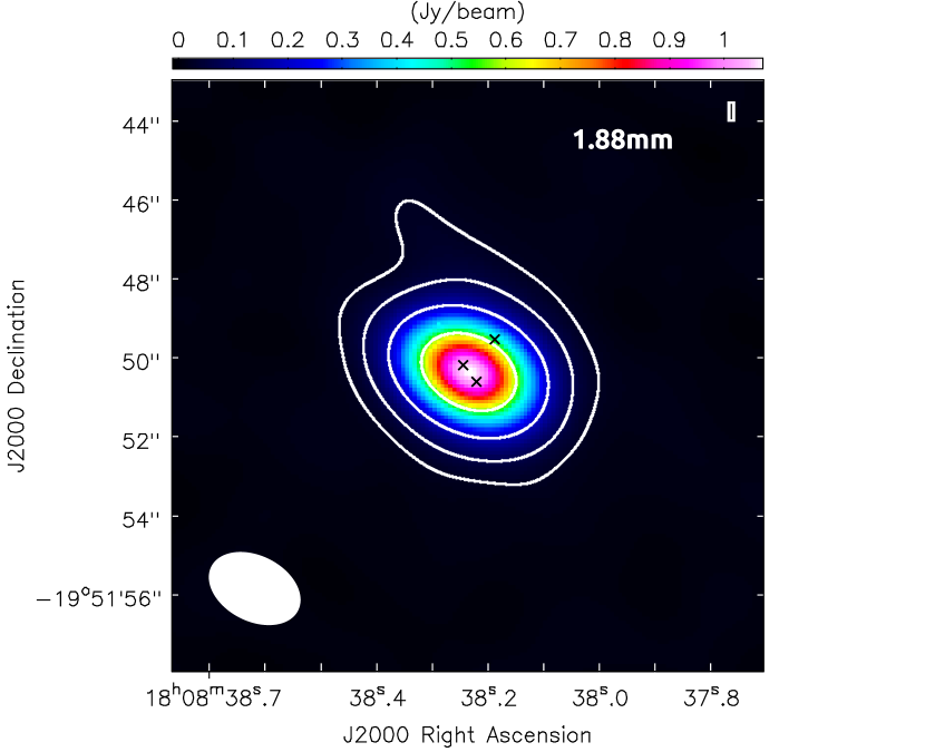
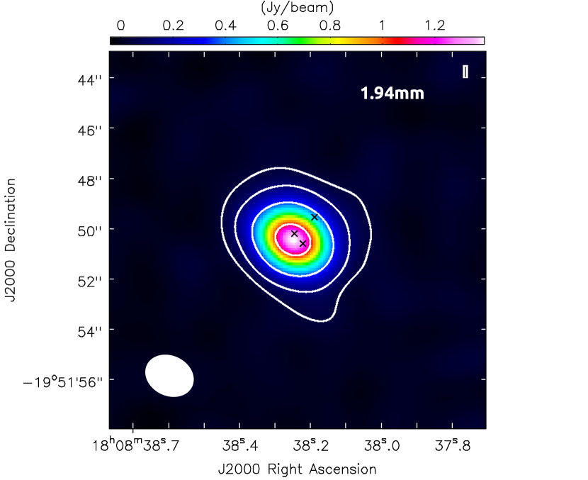
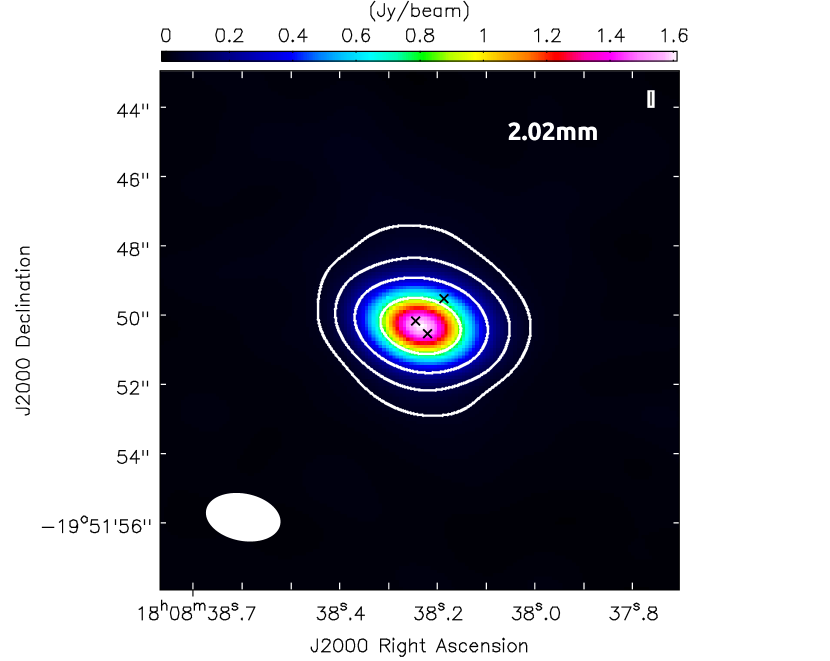
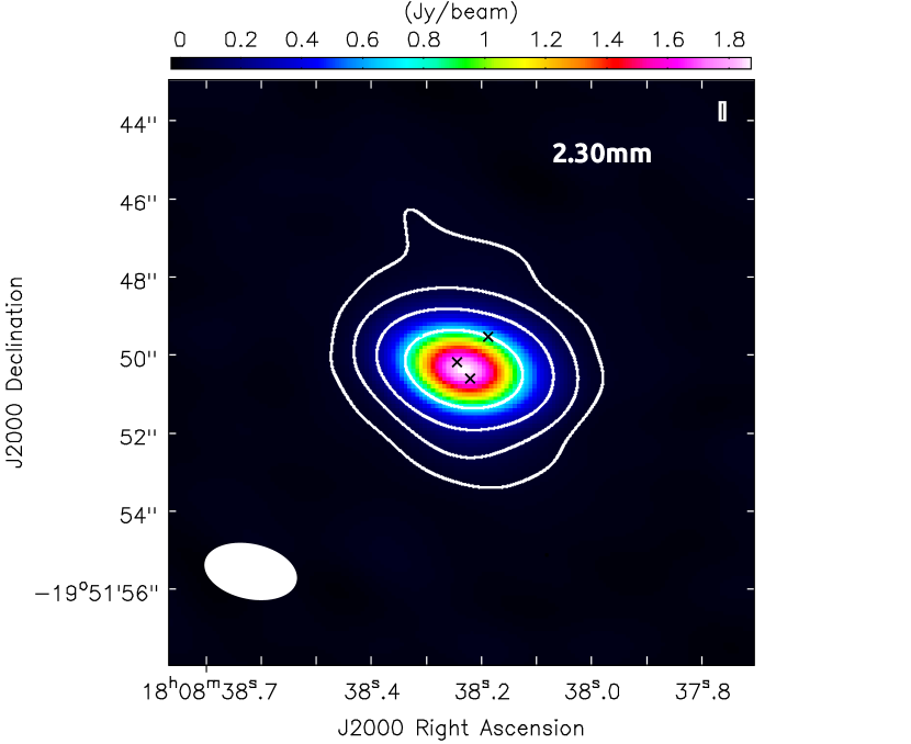
Figure 1: Images of continuum emission observed towards G10 with ALMA at (i) $130.5$ GHz ($\sigma$ = 7 mJy/beam), (ii) $148.51$ GHz ($\sigma$ = 13 mJy/beam), (iii) $153.96$ GHz ($\sigma$ = 10 mJy/beam), and (iv) $159.45$ GHz ($\sigma$ = 9 mJy/beam). Contours are drawn at 3$\sigma$, 9$\sigma$, 27$\sigma$, and 81$\sigma$ for all the continuum maps. The observed beam is shown in the lower left corner of each figure. Black crosses in the continuum images indicate the HII regions B1, B2, and A in anticlockwise direction starting from the left black cross situated in the white and pink contour of continuum images (Cesaroni et al., 2010).

Table 2: Summary of the continuum images.

Frequency	Position (ICRS 2000)		Synthesized beam	Position angle	Peak flux	Integrated flux	FWHM	RMS
(GHz)	$\alpha$, hms	$\delta$, ${\circ}$ ′ ′′	${}^{\prime\prime}\times^{\prime\prime}$	in degree	(Jy/beam)	(Jy)	′′	(mJy/beam)
130.50	18:08:38.23	-19.51.50.34	2.44$\times$1.64	63.16	1.06(0.007)	1.367(0.015)	1.04(0.057)	$7$
148.51	18:08:38.24	-19.51.50.42	1.98$\times$1.57	64.28	1.37(0.012)	2.031(0.026)	1.22(0.041)	$13$
153.96	18:08:38.24	-19.51.50.32	2.03$\times$1.47	73.50	1.59(0.001)	2.138(0.020)	1.00(0.031)	$10$
159.45	18:08:38.23	-19.51.50.35	2.38$\times$1.39	77.84	1.86(0.014)	2.477(0.030)	1.01(0.047)	$9$

Table 3: Hydrogen column density and optical depth.

Wavelength	Hydrogen column density	Optical depth
(mm)	(cm-2)	($\tau$)
2.30	$\rm{9.93\times 10^{24}}$ ($\rm{5.52\times 10^{24}}$)∗	0.098
2.02	$\rm{1.32\times 10^{25}}$ ($\rm{5.84\times 10^{24}}$)∗	0.133
1.94	$\rm{1.48\times 10^{25}}$ ($\rm{6.30\times 10^{24}}$)∗	0.151
1.88	$\rm{1.62\times 10^{25}}$ ($\rm{6.46\times 10^{24}}$)∗	0.166
Average Value	$\rm{1.35\times 10^{25}}$ ($\rm{6.04\times 10^{24}}$)∗	0.135

^∗ These are estimated by considering new set of mass absorption coefficient values, which are obtained following Motogi et al. (2019) as described in Section 3.3.

3.2 Rotation diagram analysis

In this work, we have detected multiple lines of HNCO, NH₂CHO, and CH₃NCO and carried out rotation diagram analysis to obtain the temperature and column density of the observed species. Assuming the observed transitions of these species are optically thin and are in Local Thermodynamic Equilibrium (LTE), we performed rotational diagram analysis. For optically thin lines, column density can be expressed as (Goldsmith & Langer, 1999),

$$\frac{N_{u}^{thin}}{g_{u}}=\frac{3k_{B}\int{T_{mb}dV}}{8\pi^{3}\nu S\mu^{2}},$$ (1)

where, g_u is the degeneracy of the upper state, k_B is the Boltzmann constant, $\rm{\int T_{mb}dV}$ is the integrated intensity, $\nu$ is the rest frequency, $\mu$ is the electric dipole moment, and S is the transition line strength. Under LTE conditions, the total column density can be written as,

$$\frac{N_{u}^{thin}}{g_{u}}=\frac{N_{total}}{Q(T_{rot})}\exp(-E_{u}/k_{B}T_{rot}),$$ (2)

where, $T_{rot}$ is the rotational temperature, E_u is the upper state energy, $\rm{Q(T_{rot})}$ is the partition function at rotational temperature. Equation 2 can be rearranged as,

$$log\Bigg{(}\frac{N_{u}^{thin}}{g_{u}}\Bigg{)}=-\Bigg{(}\frac{log\ e}{T_{rot}}\Bigg{)}\Bigg{(}\frac{E_{u}}{k_{B}}\Bigg{)}+log\Bigg{(}\frac{N_{total}}{Q(T_{rot})}\Bigg{)}.$$ (3)

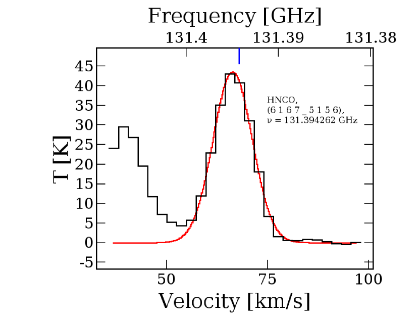
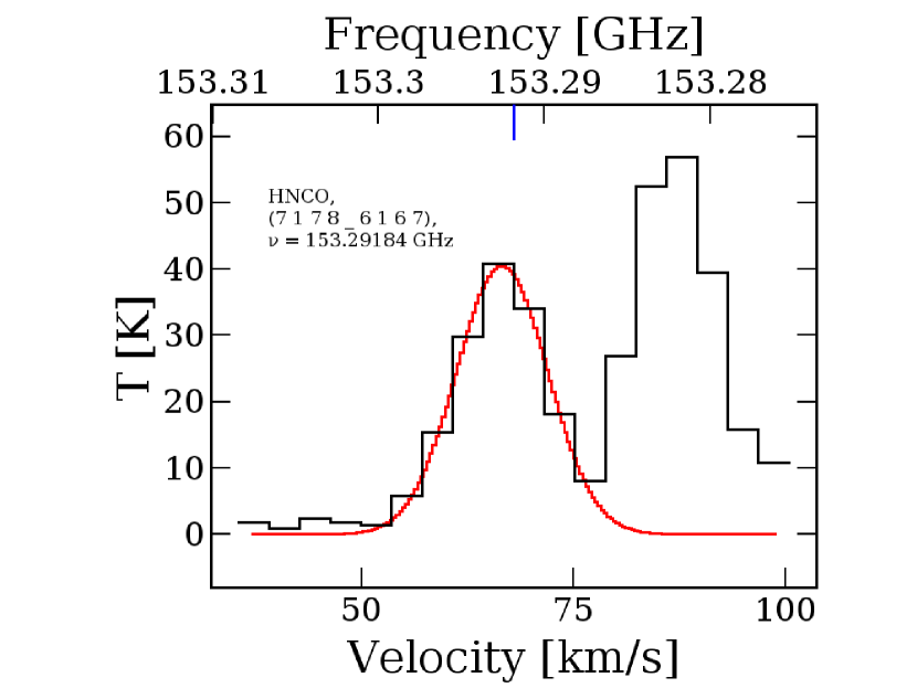
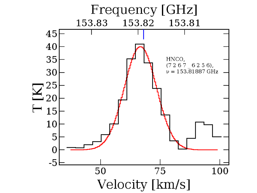
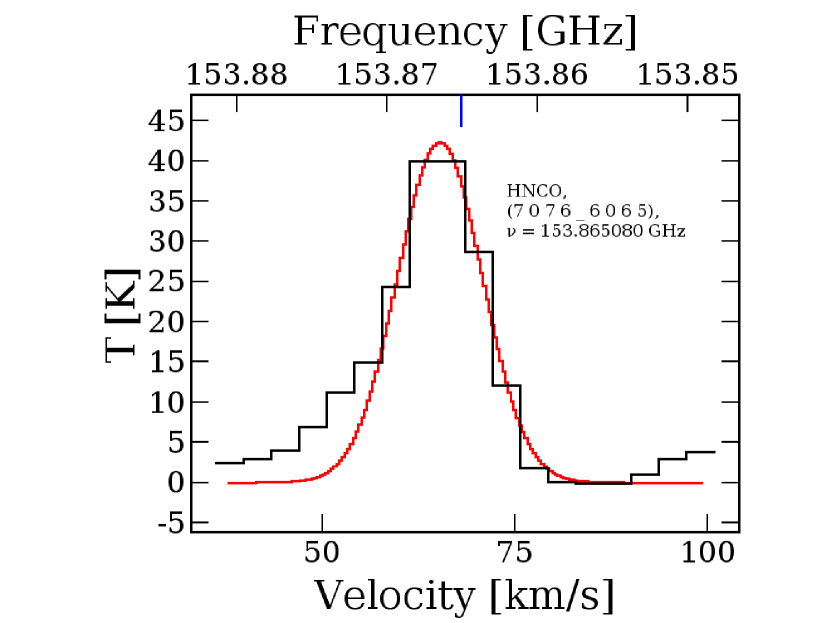
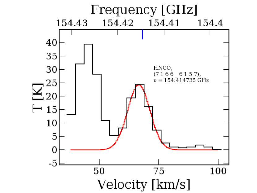
Figure 13: Gaussian fitting of the observed emission spectra of HNCO towards G10. Black line represents observed emission spectra and red line represents a Gaussian profile fitted to the observed spectra.

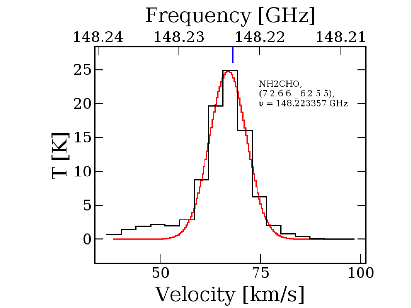
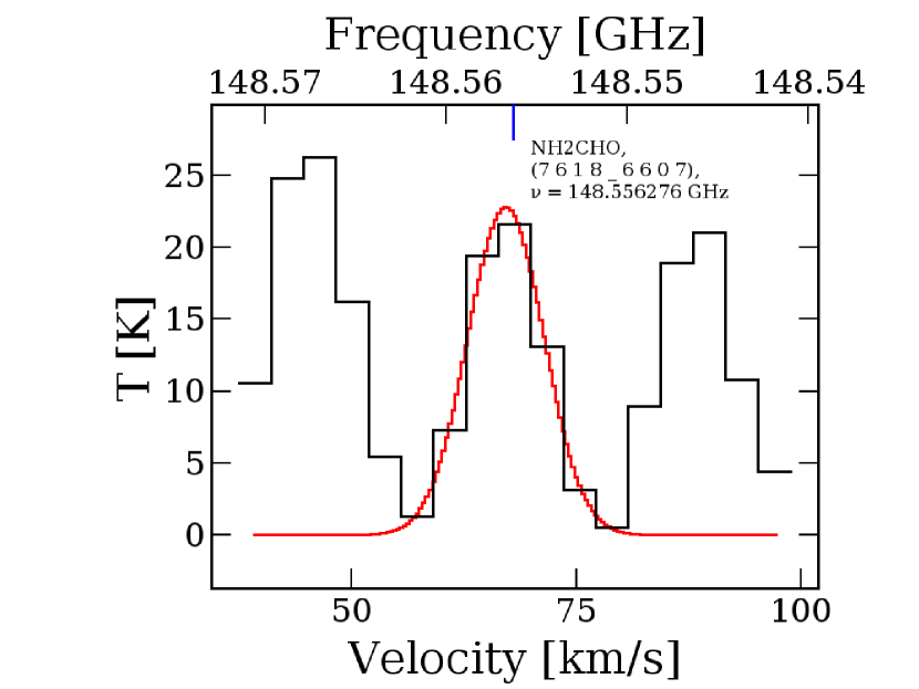
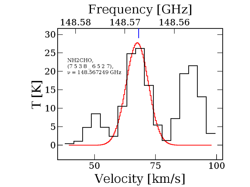
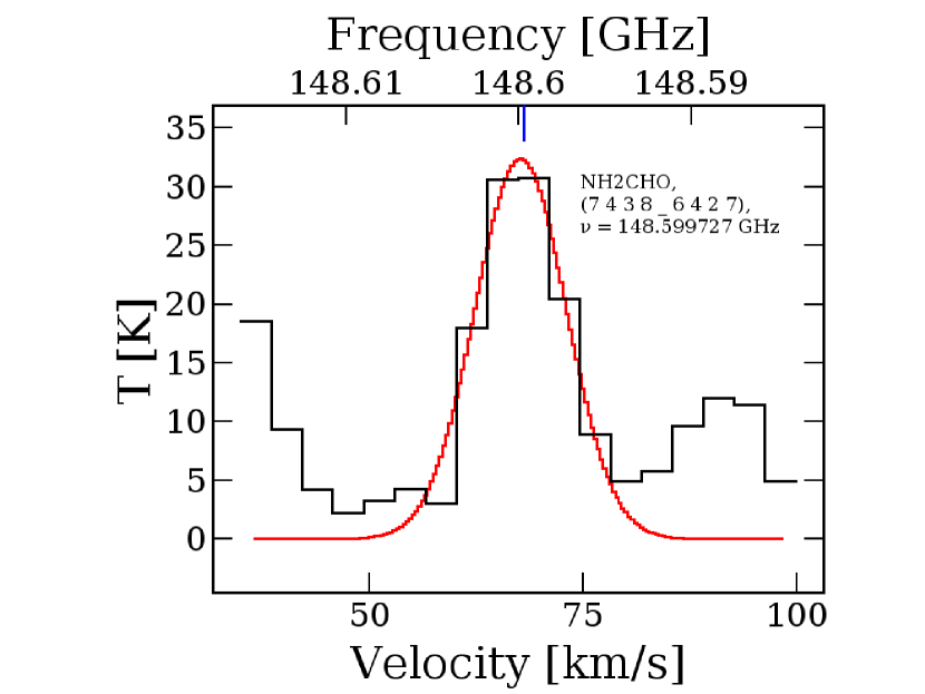
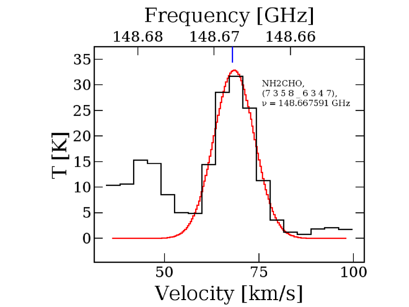
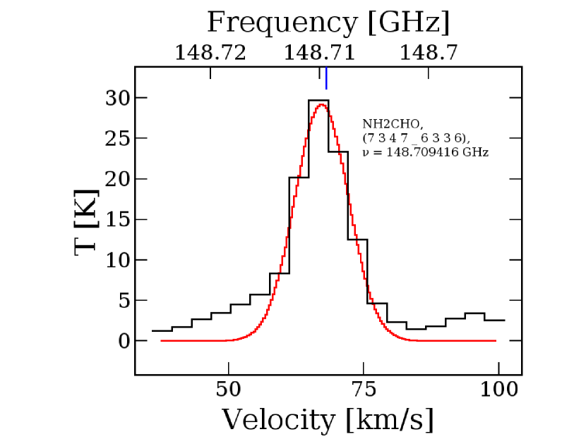
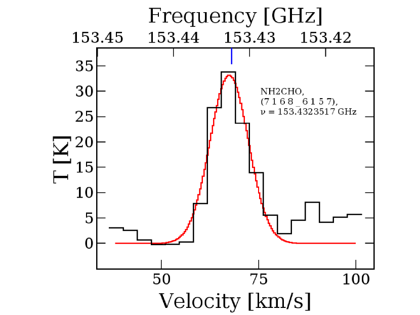
Figure 14: Gaussian fitting of the observed emission spectra of NH₂CHO towards G10. Black line represents observed emission spectra and red line represents a Gaussian profile fitted to the observed spectra.

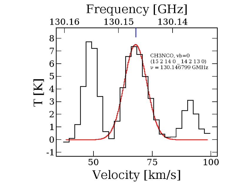
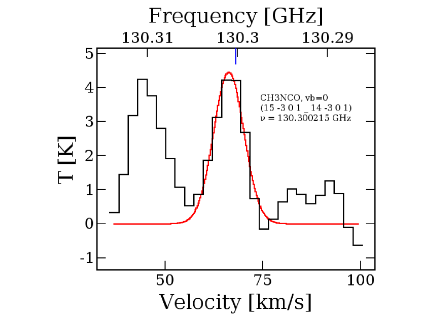
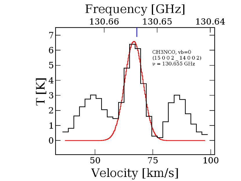
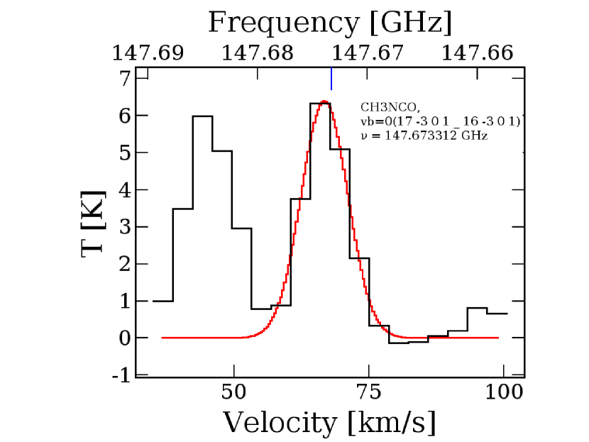
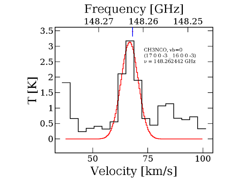
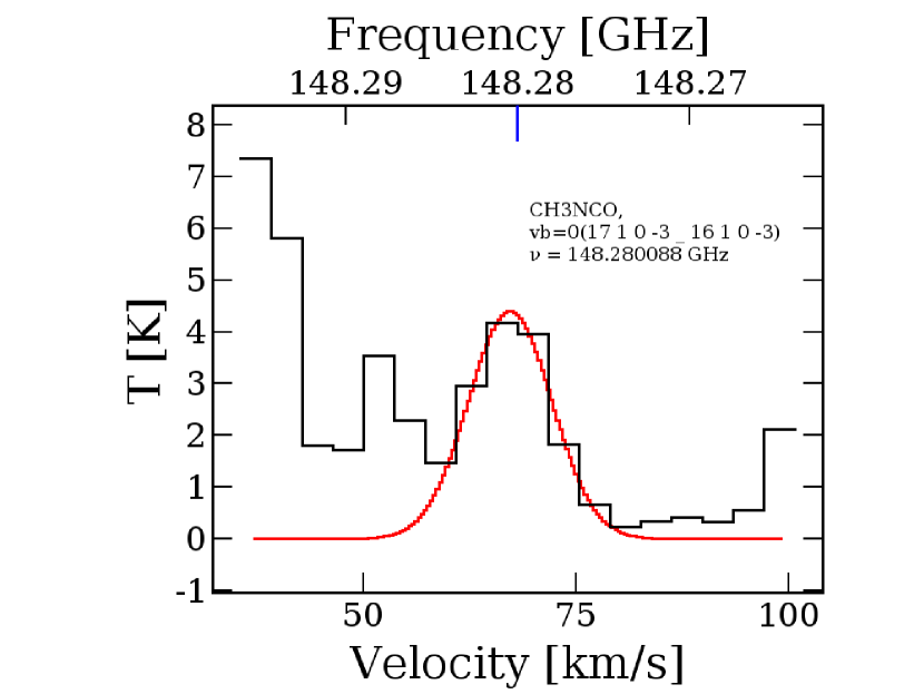
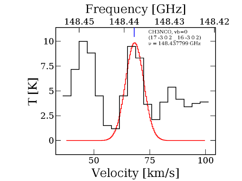
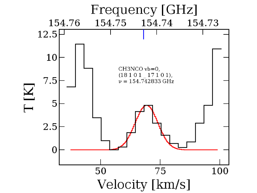
Figure 15: Gaussian fitting of the observed emission spectra of CH₃NCO towards G10. Black line represents observed emission spectra and red line represents a Gaussian profile fitted to the observed spectra.

Above equation shows that there is a linear relationship between the upper state energy and column density at the upper level. Using this equation, we can extract both column density and rotational temperature. Line parameters of the observed transitions are estimated with a single Gaussian fit. Observed and Gaussian fitted spectra of various transitions of HNCO, NH₂CHO, and CH₃NCO are provided in the Appendix (see Figures 13-15). All the line parameters of observed molecules such as molecular transitions (quantum numbers) along with their rest frequency ($\nu$), upper state energy (E_u), line width ($\Delta V$), line intensity (S$\mu^{2}$), integrated intensity ($\rm{\int T_{mb}dV}$) are presented in Table 4.

We have identified multiple hyperfine transitions of HNCO and $\rm{NH_{2}CHO}$. However, with the present spectral resolution it is not possible to resolve these transitions. Since there were various hyperfine transitions corresponds to a single observed spectral profile, we have split the observed intensity flux according to their S$\mu^{2}$ values. Then we have used the most probable (maximum intensity) hyperfine transitions in rotational diagram analysis. Selected transitions are then used to obtain the rotational temperature and column density from the rotational diagram. We have detected many transitions of CH₃NCO but few of them are blended with some other nearby molecular transitions. In Table 4, we have provided all the observed transitions. However, the integrated intensity is estimated only for non-blended transitions of CH₃NCO, which are further used in the rotational diagram analysis of it. Rotational diagrams of HNCO, NH₂CHO, and CH₃NCO are presented in Fig. 2.

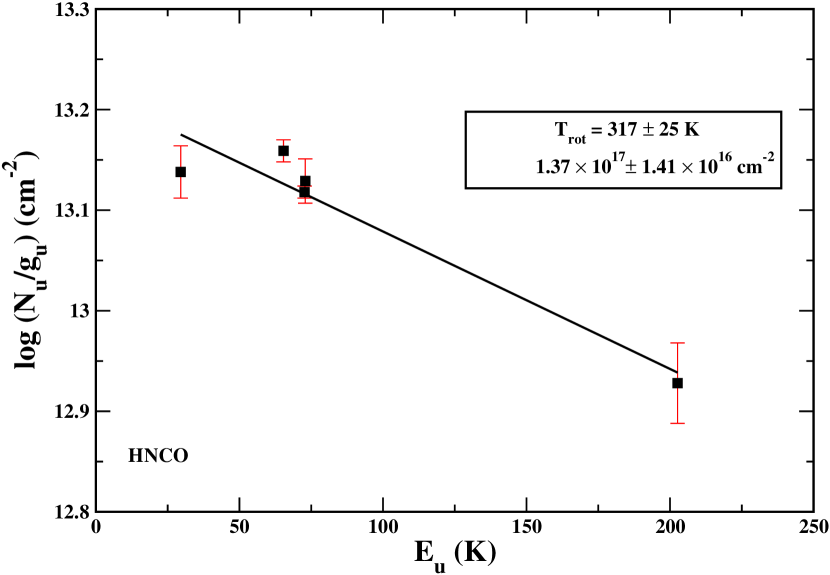
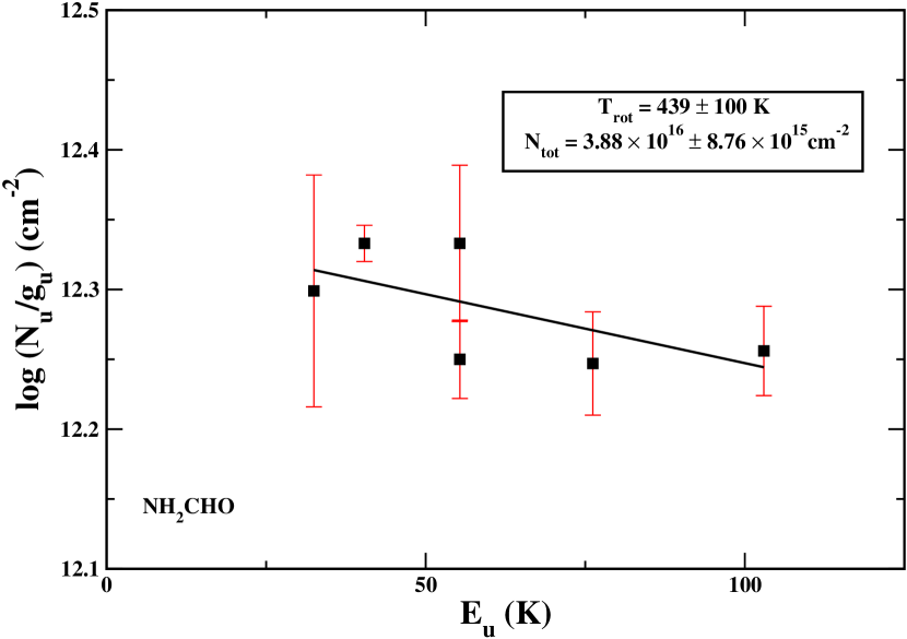
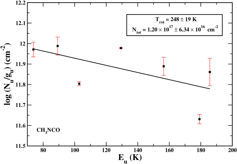
Figure 2: Rotational diagram of HNCO, NH₂CHO, and CH₃NCO. Black filled squares are the data points and red lines represent the error bar. Best fit rotational temperature and column density are mentioned inside the small box for corresponding figure.

3.3 Hydrogen Column density estimation

Flux density of the dust continuum ($S_{\nu}$) for the optically thin condition can be written as,

$$S_{\nu}=\Omega\tau_{\nu}B_{\nu}(T_{d}),$$ (4)

where, $\Omega$ is solid angle of the synthesized beam, $\tau_{\nu}$ is optical depth, $T_{d}$ is dust temperature, and $\rm{B_{\nu}(T_{d})}$ is the Planck function (Whittet, 1992). Optical depth can be expressed as,

$$\tau_{\nu}=\rho_{d}\kappa_{\nu}L,$$ (5)

where, $\rho_{d}$ is mass density of dust, $\kappa_{\nu}$ is the mass absorption coefficient, and L is the path length. Using the dust-to-gas mass ratio ($Z$), the mass density of the dust can be written as,

$$\rho_{d}=Z\mu_{H}\rho_{H_{2}}=Z\mu_{H}N_{H_{2}}2m_{H}/L,$$ (6)

where, $\rho_{H}$ is the mass density of hydrogen, N_H is the column density of hydrogen, m_H is the hydrogen mass and $\mu_{H}$ is the mean atomic mass per hydrogen. Here, we used $Z=0.01$, $\mu_{H}=1.41$ (Cox & Pilachowski, 2000), and dust temperature 200 K. Measured peak flux density of the dust continuum of the source at different frequencies are noted in Table 2. From the above equations, the column density of molecular hydrogen can be written as,

$$N_{H_{2}}=\frac{S_{\nu}/\Omega}{2\kappa_{\nu}B_{\nu}(T_{d})Z\mu_{H}m_{H}}.$$ (7)

According to the extrapolation of the data presented in Ossenkopf & Henning (1994), the mass absorption coefficient per gram of dust at $130.50$, $148.51$, $153.96$, and $159.45$ GHz ($2.30$, $2.02$, $1.94$, and $1.88$ mm respectively) is of $\sim 0.20$ cm²/g for the thin ice condition. If we adopt the formula $\rm{k_{\nu}=0.90(\nu/230GHz)^{\beta}\ cm^{2}\ g^{-1}}$ (Motogi et al., 2019) in estimating the mass absorption coefficient, where $\rm{k_{230}=0.90\ cm^{2}\ g^{-1}}$ is the emissivity of the dust grains at a gas density of $\rm{10^{6}\ cm^{-3}}$ covered by a thin ice mantle at 230 GHz. Dust spectral index $\beta$ is used of $\sim$1.6 (Friesen et al., 2005). Following the above mentioned formula, the obtained value of mass absorption coefficient is 0.36, 0.45, 0.47, and 0.50 for the frequency 130.5 GHz, 148.5 GHz, 153.96 GHz, and 159.45 GHz respectively. We estimated the hydrogen column density and optical depth of dust for the four frequency regions. Estimated hydrogen column density and optical depth values are given in Table 3. We take a mean value to find out the resultant column density of the source. By taking the average of these four continuum values, we obtained column density of $\sim 1.35\times 10^{25}$ cm^-2. Observed average hydrogen column density is of $\sim$2 times lower (see Table 3) if we consider the mass absorption coefficients values as estimated following Motogi et al. (2019). Optical depth of the dust is estimated to be $0.135$. Achieved optical depth suggests that the source is optically thin in this frequency range and with present angular resolution of the observation.

3.4 Results of observed species

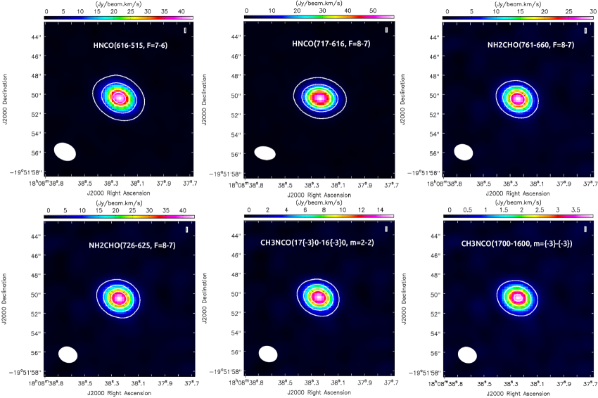
Figure 3: Moment maps of HNCO, NH₂CHO, and CH₃NCO for various transitions. The contours are from 3$\sigma$ to 43$\sigma$ in steps of 10$\sigma$ for HNCO. For $\rm{NH_{2}CHO}$ and $\rm{CH_{3}NCO}$ the contours are from 3$\sigma$ to 18$\sigma$ in steps of 5$\sigma$. The RMS noise levels are 140, 130, 282, 412, 146, and 40 mJy beam^-1 Km s^-1 for HNCO ($6_{16}-5_{15}$, $7_{17}-6_{16}$), NH₂CHO ($7_{61}-6_{60}$, $7_{26}-6_{25}$) and CH₃NCO ($17_{-30}-16_{-30}$, $17_{00}-16_{00}$) respectively.

3.4.1 Isocyanic acid, HNCO

We have observed numerous hyperfine transitions of HNCO. All the line parameters of perceived transitions are summarized in Table 4. Spatial distribution of the observed HNCO transitions is shown in Fig. 3. Here, we have depicted the spatial distribution of two transitions of HNCO with two different upper state energies. To determine the emitting region of various molecular transitions, we have used two-dimensional Gaussian fittings of the first-order moment map image. $\rm{6_{1,6}-5_{1,5}}$ emission of HNCO is found to be compact ($\rm{\theta\sim\ 1.11^{{}^{\prime\prime}}}$) than $\rm{7_{1,7}-6_{1,6}}$ transition ($\rm{\theta\sim\ 1.25^{{}^{\prime\prime}}}$). For 7_0,7-6_0,6 and 7_2,6-6_2,5 transitions we found slightly extended region ($\rm{\theta\sim\ 1.38^{{}^{\prime\prime}}}$). However, the morphological structures of spatial distribution of all transitions are similar. Obtained rotational temperature, column density, and fractional abundances are given in Table 5. From the rotational diagram analysis, we obtained a rotational temperature of about $317$ K, and column density of $\rm{\sim 1.37\times 10^{17}\ cm^{-2}}$. Gibb et al. (2003) estimated the rotational temperature and column density of HNCO to be $328$ K and 6.76$\rm{\times 10^{16}\ cm^{-2}}$ respectively in G10. Here, we obtained a column density which is about two times higher and almost similar rotational temperature as reported in Gibb et al. (2003).

3.4.2 Formamide, NH₂CHO

We have identified several hyperfine transitions of NH₂CHO. All the line parameters of the observed NH₂CHO transitions are presented in Table 4. Spatial distribution of the observed NH₂CHO transitions are depicted in Fig. 3. Spatial distribution of $\rm{7_{2,6}-6_{2,5}}$ ($E_{u}=40.40$ K) and $\rm{7_{6,1}-6_{6,0}}$ ($E_{u}=135.74$ K) transitions show similar nature. We obtained a higher rotational temperature of $\sim 439$ K. We obtained the column density of NH₂CHO of $\sim 3.88\times 10^{16}$ cm^-2 which is in good agreement with previous study (Rolffs et al., 2011). Spatial distribution of NH₂CHO is also found to be similar as HNCO. Emitting region ($\theta$) of NH₂CHO transitions varies between $\rm{1.18^{{}^{\prime\prime}}}$ and $1.55^{{}^{\prime\prime}}$.

3.4.3 Methyl isocyanate, CH₃NCO

In CH₃NCO, there is an internal rotation of the methyl group (CH₃, described by quantum number $m$) and low-frequency CNC bending motion. Estimated energies for the sub-states m = 1, 2 relative to the ground state (m = 0) is $8.4$ and $36.8$ cm^-1 respectively. For $m=3$ sub-state this estimated relative energy is $79.7$, and $80.3$ cm^-1 for the nearly two degenerate $m=3$ sub-state and $140.6$ cm^-1 for $m=4$ sub-state. The next higher vibrational state was found to be the first excited state of the CNC bending mode, $V_{b}=1$ at $182.2$ cm^-1 (Cernicharo et al., 2016). Observed transitions of CH₃NCO and their line parameters are summarized in Table 4. Several transitions of methyl isocyanate have observed in this work with $m=0,1,2,3$. Spatial distribution of CH₃NCO transitions for $m=2$ and $3$ are depicted in Figure 3. Interestingly, it is observed that emission with $m=0$ transitions of CH₃NCO are compact ($\rm{\theta\sim 1.0^{{}^{\prime\prime}}}$) with the continuum emission whereas the transitions with a higher value of m, the emitting regions are comparatively extended (for m = 1, $\rm{\theta\sim 1.15^{{}^{\prime\prime}}}$; m = 2, $\rm{\theta\sim 1.19^{{}^{\prime\prime}}}$). However, these transitions are marginally resolved and it is not possible to draw any conclusion regarding the spatial distribution of these molecules in this source. A high angular and spatial resolution observation can shed some light on this issue more elaborately. The obtained rotational temperature of CH₃NCO is $248$ K. For another high-mass star-forming region, Cernicharo et al. (2016) observed CH₃NCO in the warm gas of Sgr B2 and obtained rotational temperature of $\sim$ 200 K and column density of $\sim\rm{(3-5)\times 10^{17}\ cm^{-2}}$. We estimated the column density and fractional abundance CH₃NCO as $\rm{1.20\times 10^{16}}$ cm^-2 and $\rm{8.88\times 10^{-09}}$ respectively. Our observed column density of CH₃NCO in this source to be 2-4 times lower as compared to that in Sgr B2 observation (Cernicharo et al., 2016).

Table 4: Summary of the line parameters of observed molecules towards G10.

Species	(${\rm J^{{}^{\prime}}_{K_{a}^{{}^{\prime}}K_{c}^{{}^{\prime}}}}$-${\rm J^{{}^{\prime\prime}}_{K_{a}^{{}^{\prime\prime}}K_{c}^{{}^{\prime\prime}}}}$)	Frequency (GHz)	Eu (K)	FWHM (Km s-1)	S$\mu^{2}$(Debye2)	${\int{T_{mb}}dv(K.Km/s)}$	Remarks
	61,6-51,5, F=7-6	131.394262	65.35	3.85	0.00291	228.88$\pm$5.72
HNCO	71,7-61,6, F=8-7	154.414770	72.92	1.93	0.35919	289.88$\pm$12.91
	70,7-60,6, F=8-7	153.865080	29.54	2.27	0.36664	301.17$\pm$17.68
	72,6-62,5, F=8-7	153.818870	202.63	1.99	0.33673	170.14$\pm$14.40
	71,7-61,6, F=8-7	153.291840	72.70	2.16	0.00184	280.76$\pm$3.66
	72,6-62,5, F= 8-7	148.223354	40.40	3.79	95.26	212.49$\pm$6.33
	76,1-66,0, F=8-7	148.556276	135.74	1.71	20.55	74.04$\pm$6.22
	75,3-65,2, F=8-7	148.567249	102.99	1.81	43.92	95.13$\pm$6.96
NH2CHO	74,3-64,2, F=8-7	148.599727	76.19	2.11	52.15	128.08$\pm$11.02
	73,5-63,4, F=8-7	148.667591	55.34	4.23	73.20	189.77$\pm$12.34
	73,4-63,3, F=8-7	148.709316	55.35	3.93	63.22	161.56$\pm$10.54
	71,6-61,5, F=8-7	153.432351	32.47	3.82	101.58	217.18$\pm$41.43
	150,15-140,14, m=0-0	129.957471	49.91	–	123.94	–	Blended
	153,12-143,11, m=0-0	129.669703	103.61	–	120.32	–	Blended
	152,14-142,13, m=0-0	130.146799	73.80	11.63	121.88	103.58$\pm$8.52
	15-3,0- 14-3,0, m=1-1	130.300215	115.63	9.61		50.89$\pm$5.36
	152,13-142,12, m=0-0	130.228419	73.82	–	121.89	–	Blended
	152,0-142,0, m=1-1	130.541066	85.84	–	121.08	–	Blended
	15-1,0-14-10, m=2-2	130.583038	108.84	–	122.79	–	Blended
	150,0-140,0, m=2-2	130.653851	102.88	9.39	123.19	71.61$\pm$1.57
	143,0-133,0, m=1-1	130.661691	109.38	–	95.64	–	Blended
	151,0-141,0, m=2-2	130.88332	108.84	–	124.79	–	Blended
CH3NCO	173,0 -163,0, m=(-3)-(-3)	148.833657	232.81	–	122.25	–	Blended
	17-3,0 -16-3,0, m=2-2	148.437799	170.22	9.92	134.84	200.34$\pm$9.84
	171,0-1610, m=2-2	148.376092	85.19	–	138.51	–	Blended
	171,0-161,0, m=3-3	148.326896	184.87	–	141.48	–	Blended
	171,0-161,0, m=(-3)-(-3)	148.280088	185.73	12.11	141.57	106.45$\pm$16.28
	170,0-160,0, m=(-3)-(-3)	148.262442	179.18	10.03	139.37	61.71$\pm$3.20
	163,0-153,0, m=1-1	148.075687	122.28	–	112.35	–	Blended
	170,0-160,0, m=2-2	148.061901	116.62	–	139.59	–	Blended
	17-3,0 -16-3,0, m=1-1	147.673312	129.36	10.53	136.04	133.62$\pm$0.98
	172,15-162,14, m=0-0	147.603962	87.56	–	138.69	–	Blended
	181,0-171,1, m=1-1	154.742833	89.20	11.62	150.95	158.88$\pm$15.98
	181,18-171,17, m=0-0	154.636867	76.47	–	148.31	–	Blended

Table 5: Estimated rotational temperatures, column densities, and fractional abundances of the observed species.

Species	Rotational	Column	Fractional
	temperature	density	abundance
	(K)	(cm-2)
HNCO	317 $\pm$ 25	$\rm{1.37\times 10^{17}}$	$\rm{1.02\times 10^{-08}}$
NH2CHO	439 $\pm$ 100	$\rm{3.88\times 10^{16}}$	$\rm{2.87\times 10^{-09}}$
CH3NCO	248 $\pm$ 19	$\rm{1.20\times 10^{17}}$	$\rm{8.88\times 10^{-09}}$

Notes. Assuming the mean value of $\rm{N_{H_{2}}=1.35\times 10^{25}}$ cm^-2 as estimated in Table 3.

3.5 LTE fitting using MCMC

We have used Markov Chain Monte Carlo (MCMC) method to fit the observed line profiles of $\rm{HNCO,NH_{2}CHO}$, and $\rm{CH_{3}NCO}$ towards the hot core G10. We have assumed that the source is under the LTE condition. We have extracted the best fitted physical parameters (column density, excitation temperature, FWHM, optical depth, and source velocity) from the fitting. We have used the python scripting interface available in CASSIS for our model calculation to find out the best-fitted physical parameters for the astronomical source. To determine the best-fitted set that can fit the observational result, we have used the $\chi^{2}$ minimization process by considering the N number of spectra. This python script computes the $\chi^{2}$ between the observed and simulated data and finds the minimal value of $\chi^{2}$ following the relation:

$${\rm{\chi_{i}}^{2}=\sum_{j=1}^{N_{i}}\frac{(I_{obs,ij}-I_{model,ij})^{2}}{rms^{2}_{i}+(cal_{i}\times I_{obs,ij})^{2}}},$$

where, ${\rm I_{obs,ij}}$ and ${\rm I_{model,ij}}$ are observed and modeled intensity in the channel j of transition i respectively, rms_i is the rms of the spectrum i, and cal_i is the calibration error. The reduced $\chi^{2}$ is computed using the following relation:

$${\rm\chi^{2}_{red}=\frac{1}{\sum_{i}^{N_{spec}}N_{i}}\sum_{i=1}^{N_{spec}}\chi^{2}_{i}}.$$

In the MCMC calculation, the initial physical values are chosen randomly between the minimum (${\rm X_{max}}$) to the maximum (${\rm X_{min}}$) range set by the user during their modeling. The step of MCMC computation ($\theta_{l}$) depends on the iteration number $l$ and other parameters ($\alpha$ and $v$), where, $\theta_{l+1}=\theta_{l}+\alpha(v-0.05)$ (v is a random number between 0 to 1). Here $\alpha$ is defined as,

$${\rm\alpha=\frac{k(X_{max}-X_{min})}{k^{\prime}}},$$

where, k is defined as

$$k=r_{c}\hskip 99.58464pt\rm{when\ l>c},$$

$$k=\frac{(r_{c}-1)}{c}l+1\hskip 56.9055pt\rm{when\ l<c},$$

where, c and r_c are the parameter cutoff and ratio at cutoff respectively which are set by the user during the modeling. k^′ is defined as reduced physical parameter which is set to a value during computation. $\alpha$ determines the amplitude of the steps, which starts with a bigger step at the initial stage of the computation to find a good $\chi^{2}$ and shorter steps at the end of the computation to extract the value of the potential best $\chi^{2}$.

LTE model fitted line parameters of all the observed transitions are provided in Table 6. The observed spectra, along with the fitted one, are shown in Fig. 4, 5, and 6 for $\rm{HNCO}$, $\rm{NH_{2}CHO}$, and $\rm{CH_{3}NCO}$ respectively. We found that some transitions of $\rm{CH_{3}NCO}$ are blended and thus, we do not obtain better fits for those transitions. Some of the spectra shown in these figures contain multiple hyperfine transitions. For the LTE fitting, we have considered only that transition which has the highest value of Einstein coefficients among them. Since some of the transitions with the highest Einstein coefficient are slightly offset from the peak position, LTE fitting results show a slight offset from some observational spectra. Extracted physical parameters in Table 6 shows that the optical depths ($\tau$) of all the lines are less than $1$. Our obtained best fitted column densities of these three species are shown in Table 6. For this MCMC fitting, we have used the different source sizes for different species as obtained from their two-dimensional Gaussian fitting. We have obtained higher excitation temperatures by the MCMC calculations (Table 6) which are consistent with the high rotational temperatures of these molecules obtained by the rotational diagram analysis which is described in the Section 3.2 (Table 5).

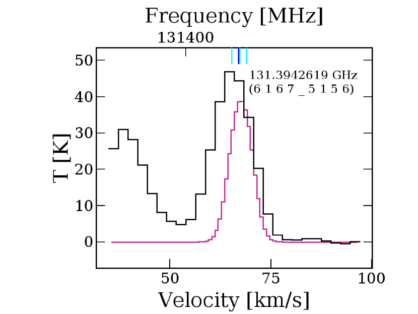
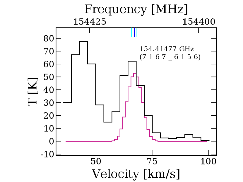
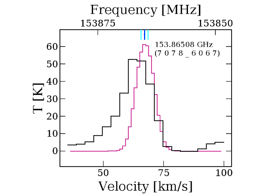
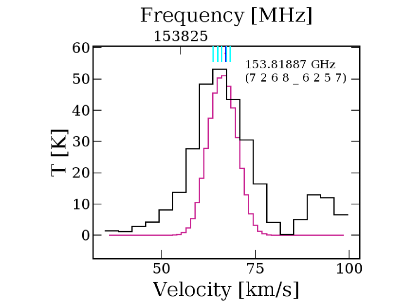
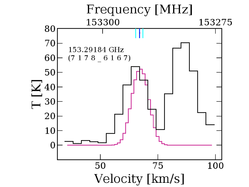
Figure 4: LTE fitting of observed lines of HNCO towards G10. Black line represents the observed spectra and pink line is the fitted profile.

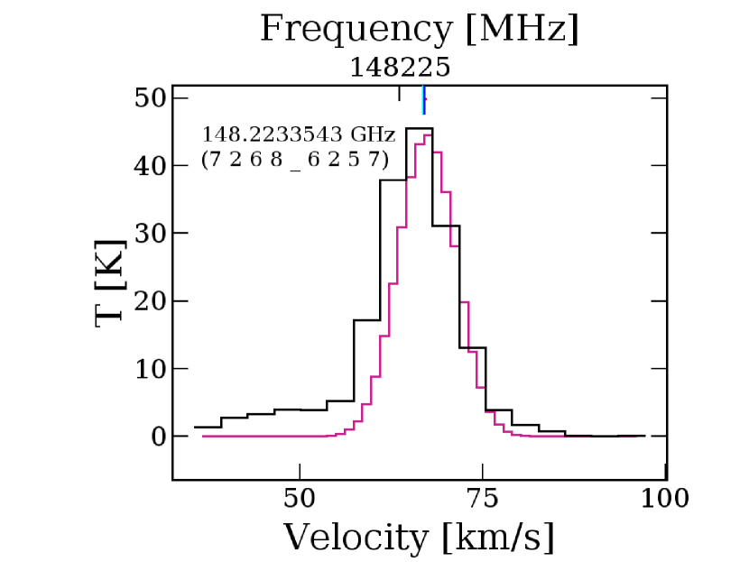
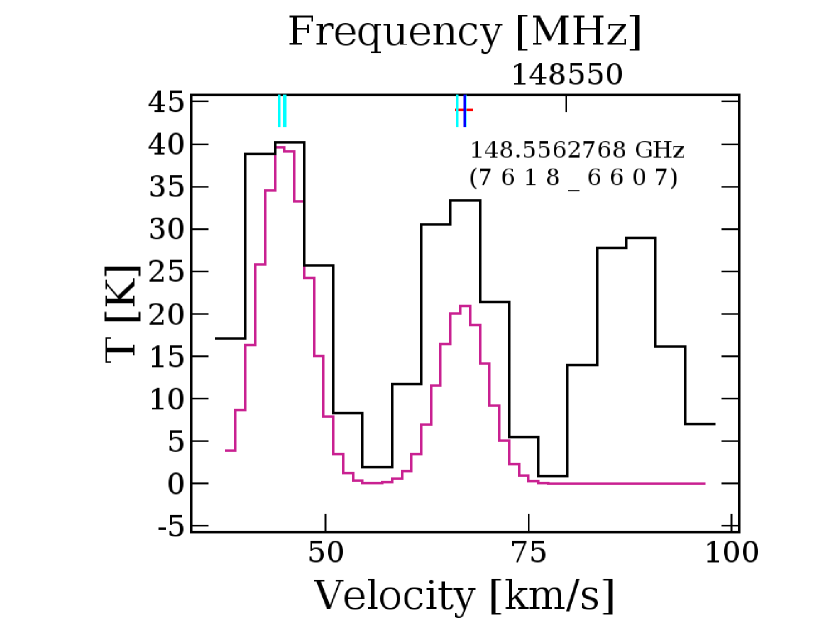
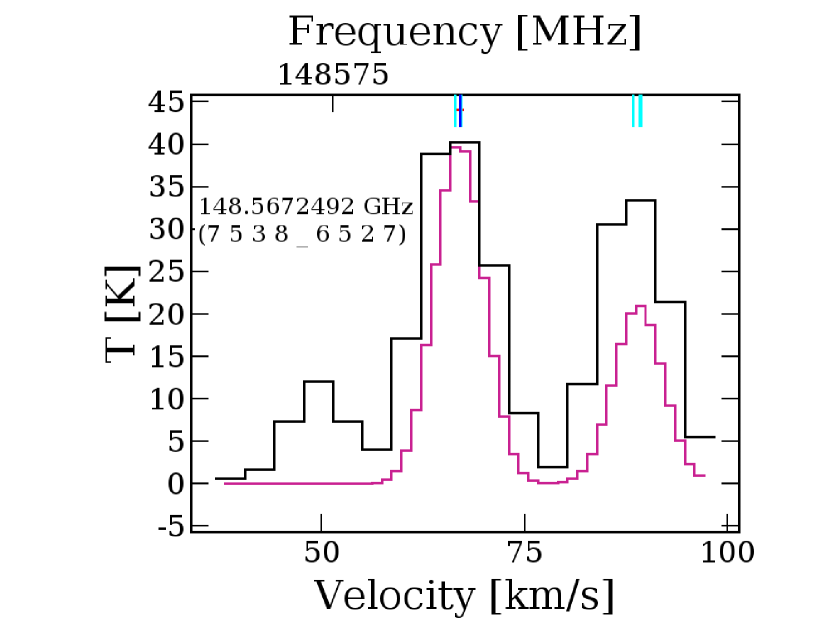
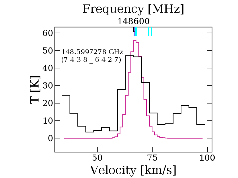
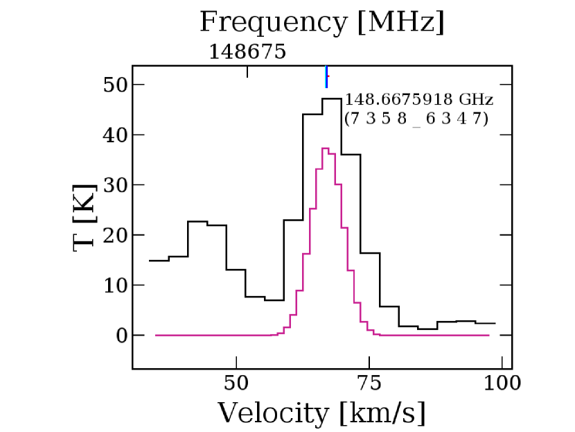
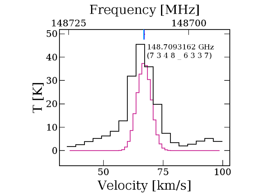
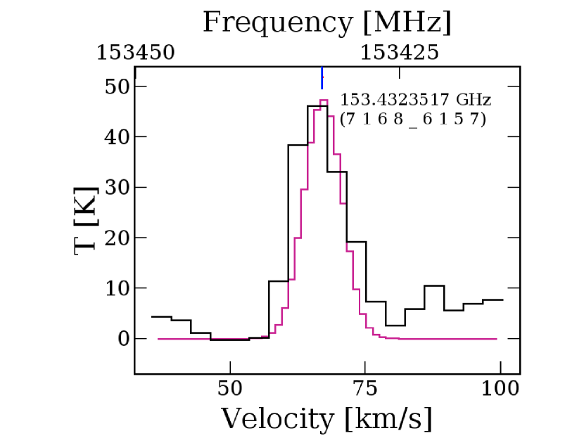
Figure 5: LTE fitting of observed lines of $\rm{NH_{2}CHO}$ towards G10. Black line represents the observed spectra and pink line is the fitted profile.

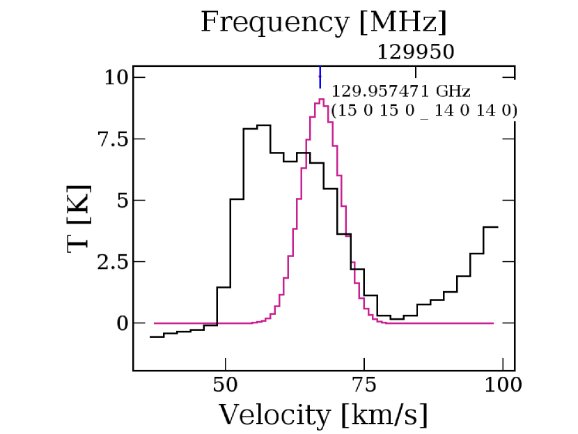
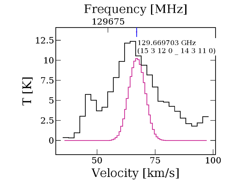
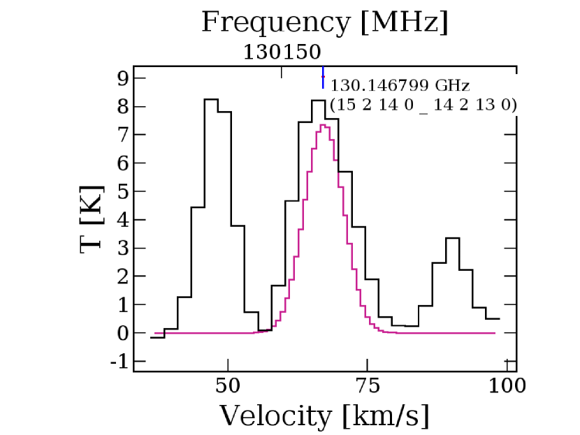
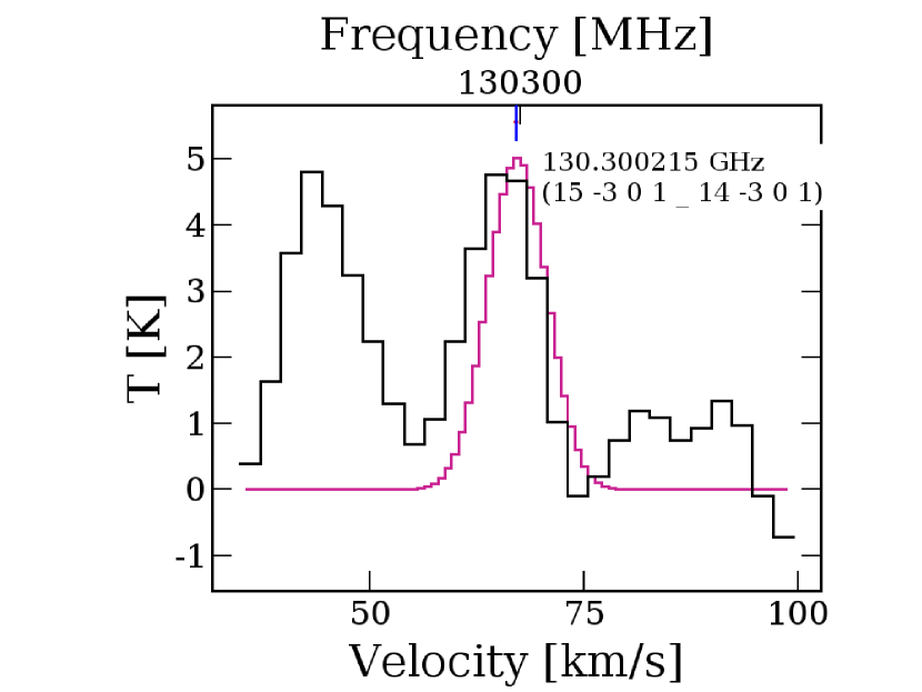
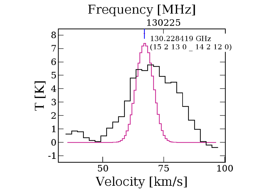
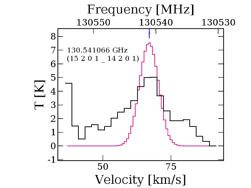
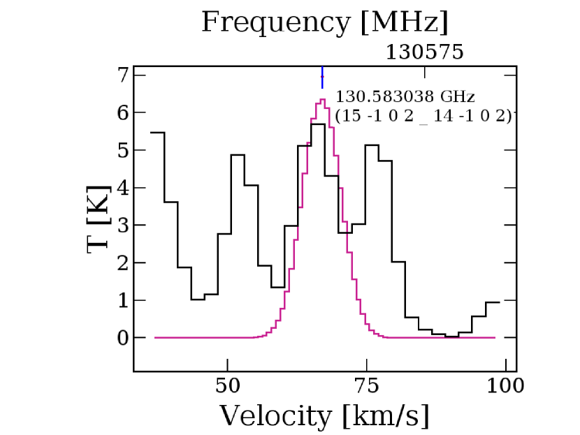
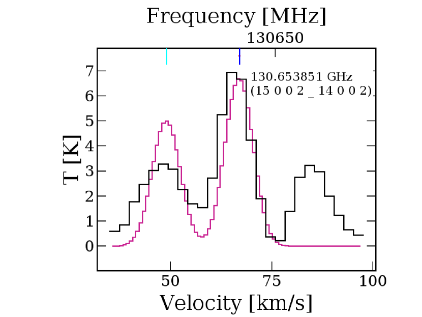
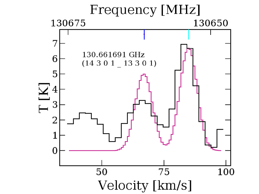
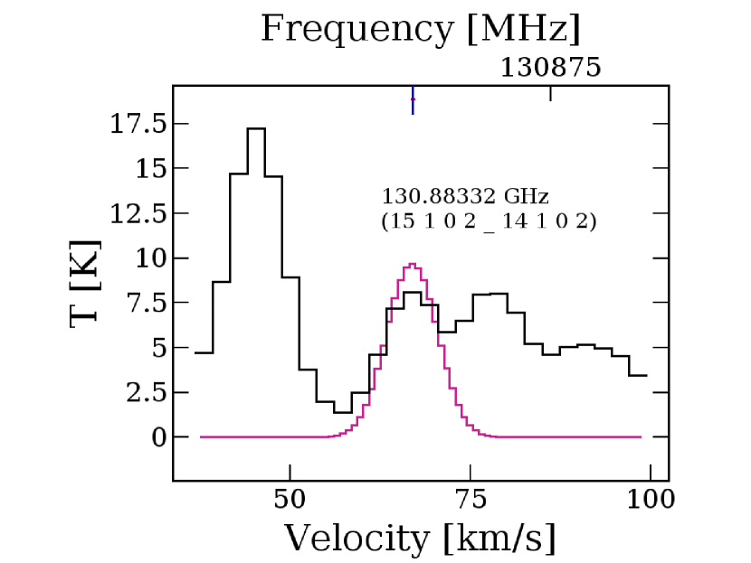
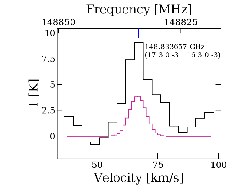
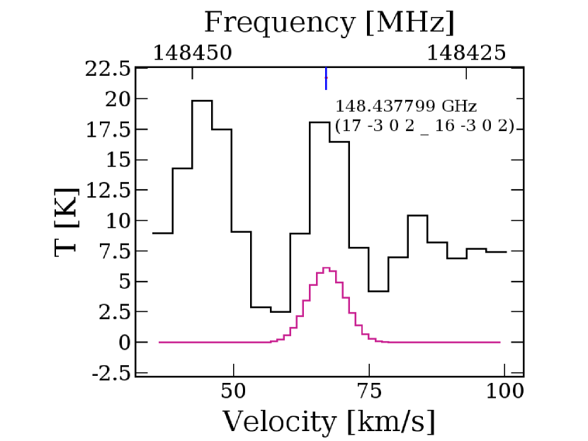
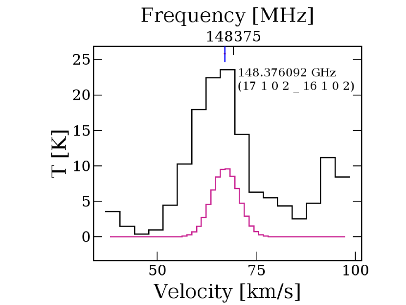
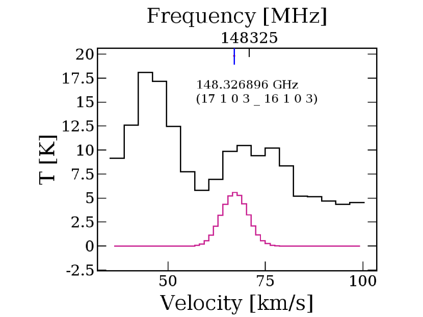
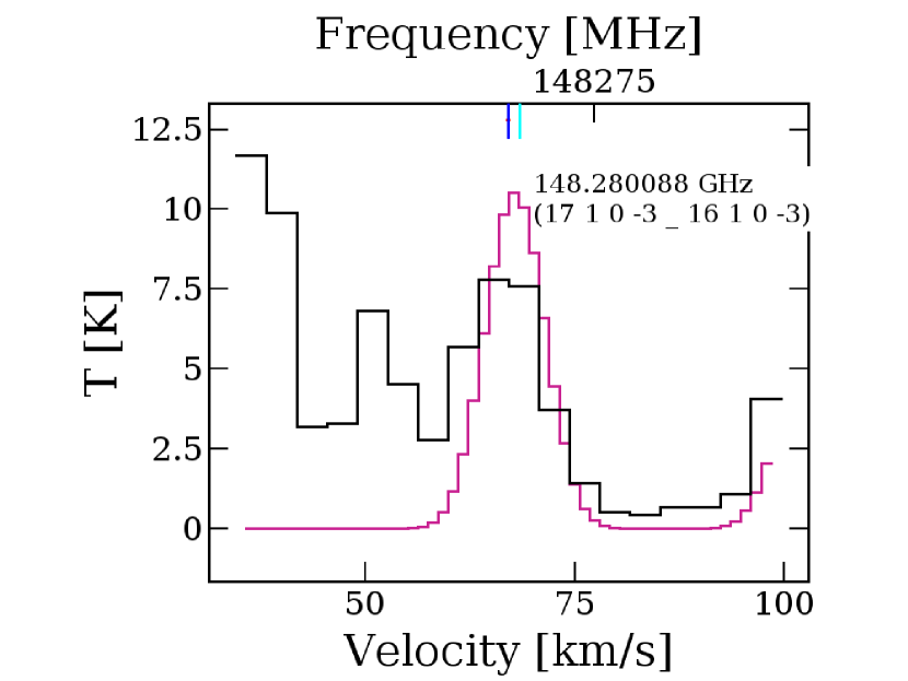
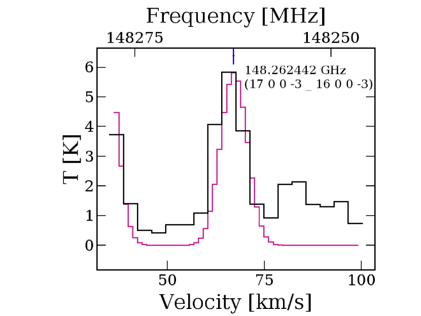
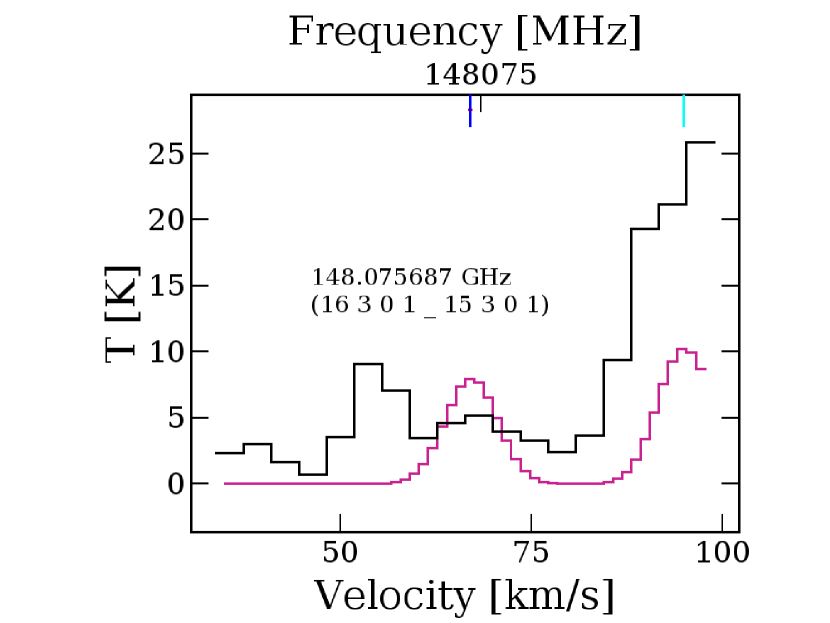
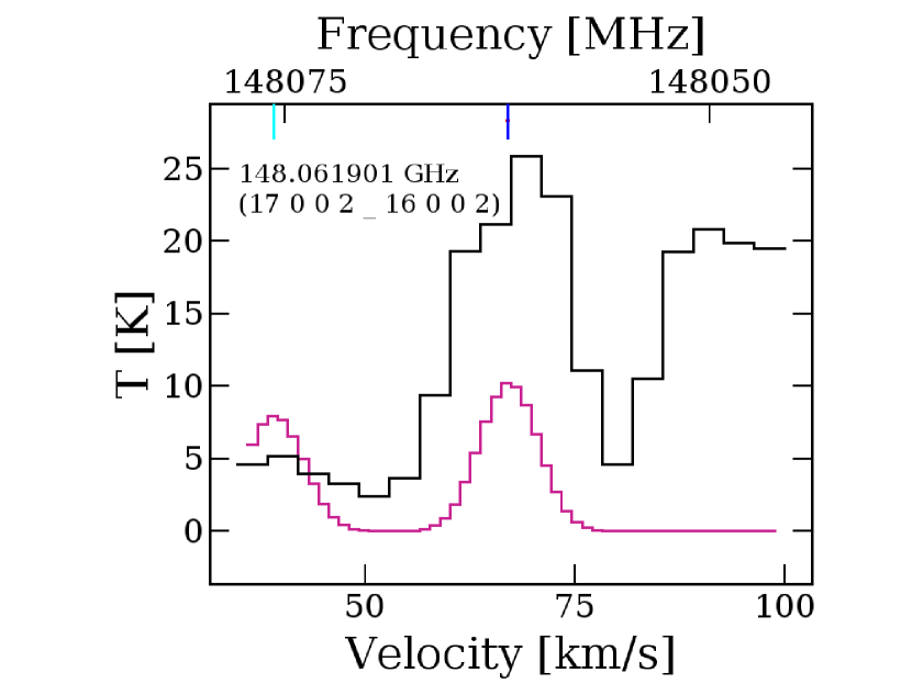
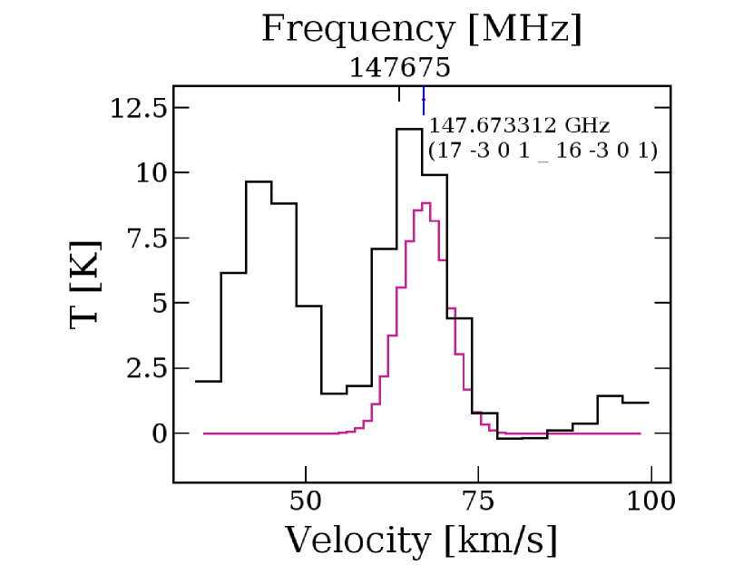
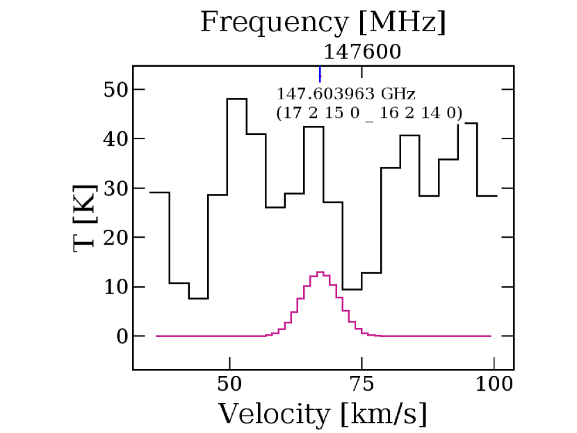
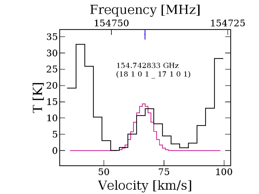
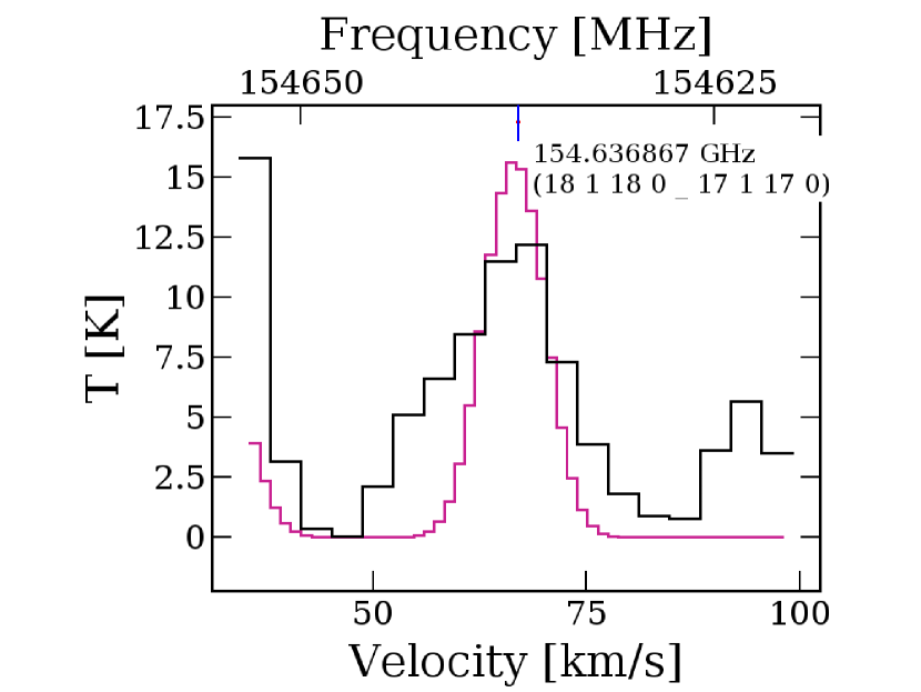
Figure 6: LTE fitting of observed transitions of $\rm{CH_{3}NCO}$ towards G10. Black line represents the observed spectra and pink line is the fitted profile.

Table 6: Summary of the best fitted line parameters of observed molecules towards G10.

Species	Frequency	Range used	Range used	Best fit FWHM	Best fit column	Optical depth	Range used	Best fitted	Source size	Range used	Best fitted
	(GHz)	Frequency (GHz)	FWHM (Km s-1)	(Km s-1)	density (cm-2)	($\tau$)	Tex (K)	Tex (K)	(${}^{{}^{\prime\prime}}$)	Vlsr (Km s-1)	Vlsr (Km s-1)
	131.394262	130.53092 - 131.46660	3-6	5.97	1.6$\times$1017	2.85$\times$10-1	200-350	201.19	1.12	67.2-67.9	67.59
HNCO	154.414770	154.03118 - 154.96636	5-7	6.97	1.6$\times$1017	2.64$\times$10-1	200-350	205.65	1.16	66.5-67.5	67.20
	153.865080	153.03117 - 153.96523	5-8	7.96	1.5$\times$1017	2.94$\times$10-1	200-330	211.98	1.35	66.5-67.5	67.32
	153.818870	153.03117 - 153.96523	5-8	7.96	1.5$\times$1017	1.19$\times$10-1	200-330	211.98	1.35	66.5-67.5	67.32
	153.291840	153.03117 - 153.96523	5-8	7.96	1.5$\times$1017	2.34$\times$10-1	200-330	211.98	1.35	66.5-67.5	67.32
	148.223354	148.46523 - 147.53117	3-9	8.98	1.3$\times$1017	7.73$\times$10-2	400-600	472.07	1.33	66.5-67.5	67.43
	148.556276	148.53115 - 149.46522	3-7	7.00	9.5$\times$1016	1.78$\times$10-2	400-550	450.09	1.37	66.5-67.5	67.09
	148.567249	148.53115 - 149.46522	3-7	7.00	9.5$\times$1016	3.52$\times$10-2	400-550	450.09	1.37	66.5-67.5	67.09
NH2CHO	148.599727	148.53115 - 149.46522	3-7	7.00	9.5$\times$1016	5.15$\times$10-2	400-550	450.09	1.37	66.5-67.5	67.09
	148.667591	148.53115 - 149.46522	3-7	7.00	9.5$\times$1016	6.53$\times$10-2	400-550	450.09	1.37	66.5-67.5	67.09
	148.709316	148.53115 - 149.46522	3-7	7.00	9.5$\times$1016	6.54$\times$10-2	400-550	450.09	1.37	66.5-67.5	67.09
	153.432351	153.96523 - 153.03118	3-8	7.99	1.2$\times$1017	6.70$\times$10-2	400-600	474.33	1.18	66.5-67.5	67.43
	129.957471	129.53092 - 130.46674	4-8	7.99	6.9$\times$1016	3.08$\times$10-1	100-300	104.04	1.05	66.5-67.5	67.14
	129.669703	129.53092 - 130.46674	4-8	7.99	6.9$\times$1016	1.77$\times$10-1	100-300	104.04	1.05	66.5-67.5	67.14
	130.146799	129.53092 - 130.46674	4-8	7.99	6.9$\times$1016	2.41$\times$10-1	100-300	104.04	1.05	66.5-67.5	67.14
	130.300215	129.53092 - 130.46674	4-8	7.99	6.9$\times$1016	1.57$\times$10-1	100-300	104.04	1.05	66.5-67.5	67.14
	130.228419	129.53092 - 130.46674	4-8	7.99	6.9$\times$1016	2.41$\times$10-1	100-300	104.04	1.05	66.5-67.5	67.14
	130.541066	130.53092 - 131.46660	4-8	5.99	7.8$\times$1016	1.91$\times$10-1	100-300	115.48	1.15	66.5-67.5	66.89
	130.583038	130.53092 - 131.46660	4-8	7.99	7.8$\times$1016	1.59$\times$10-1	100-300	115.48	1.15	66.5-67.5	66.89
	130.653851	130.53092 - 131.46660	4-8	7.99	7.8$\times$1016	1.68$\times$10-1	100-300	115.48	1.15	66.5-67.5	66.89
	130.661691	130.53092 - 131.46660	4-8	7.99	7.8$\times$1016	1.23$\times$10-1	100-300	115.48	1.15	66.5-67.5	66.89
	130.88332	130.53092 - 131.46660	4-8	7.99	7.8$\times$1016	1.58$\times$10-1	100-300	115.48	1.15	66.5-67.5	66.89
CH3NCO	148.833657	148.53115 - 149.46522	4-8	7.99	8.8$\times$1016	7.25$\times$10-2	100-300	122.21	1.23	66.5-67.5	66.68
	148.437799	148.46523 - 147.53117	4-8	7.92	7.7$\times$1016	1.41$\times$10-1	100-300	101.24	1.23	66.5-67.5	67.13
	148.376092	148.46523 - 147.53117	4-8	7.92	7.7$\times$1016	2.32$\times$10-1	100-300	101.24	1.23	66.5-67.5	67.13
	148.326896	148.46523 - 147.53117	4-8	7.92	7.7$\times$1016	1.28$\times$10-1	100-300	101.24	1.23	66.5-67.5	67.13
	148.280088	148.46523 - 147.53117	4-8	7.92	7.7$\times$1016	1.27$\times$10-1	100-300	101.24	1.23	66.5-67.5	67.13
	148.262442	148.46523 - 147.53117	4-8	7.92	7.7$\times$1016	1.33$\times$10-1	100-300	101.24	1.23	66.5-67.5	67.13
	148.075687	148.46523 - 147.53117	4-8	7.92	7.7$\times$1016	1.88$\times$10-1	100-300	101.24	1.23	66.5-67.5	67.13
	148.061901	148.46523 - 147.53117	4-8	7.92	7.7$\times$1016	2.48$\times$10-1	100-300	101.24	1.23	66.5-67.5	67.13
	147.673312	148.46523 - 147.53117	4-8	7.92	7.7$\times$1016	2.12$\times$10-1	100-300	101.24	1.23	66.5-67.5	67.13
	147.603962	148.46523 - 147.53117	4-8	7.92	7.7$\times$1016	3.27$\times$10-1	100-300	101.24	1.23	66.5-67.5	67.13
	154.742833	154.03118 - 154.96636	4-8	7.97	7.5$\times$1016	3.53$\times$10-1	100-300	101.70	1.21	66.5-67.5	66.54
	154.636867	154.03118 - 154.96636	4-8	7.97	7.5$\times$1016	3.92$\times$10-1	100-200	101.70	1.21	66.5-67.5	66.54

4 Chemical Modeling

We carry out extensive modeling to study the abundance of three peptide bond related species in G10. To study the chemical evolution of these species, we used our previous chemical network (Das et al., 2015a, b, 2016; Gorai et al., 2017a, b; Sil et al., 2018). Gas phase pathways were mainly adopted from the UMIST database (McElroy et al., 2013), whereas ice phase pathways and binding energies (BEs) of the surface species were taken from the KIDA database (unless otherwise stated, Ruaud et al., 2016). We have considered the diffusion energy of a species is $0.5$ times its adsorption energy and non-thermal desorption rate with a fiducial parameter $0.01$ (Gorai et al., 2017a). A cosmic ray rate of $1.3\times 10^{-17}$ s^-1 is considered in all our models. For the formation and destruction reactions of these species, we mainly have followed Quénard et al. (2018). In addition, following the recent study of Haupa et al. (2019), we have exclusively included a dual-cyclic hydrogen addition and abstraction reactions, which is connecting NH₂CHO, NH₂CO, and HNCO. We have shown the chemical linkages among HNCO, NH₂CHO, and CH₃NCO. Initial abundances of the model is provided in Table 7.

Table 7: Initial abundances with respect to total hydrogen nuclei.

Species	Abundance
$\mathrm{H_{2}}$	$5.00\times 10^{-01}$
$\mathrm{He}$	$9.00\times 10^{-02}$
$\mathrm{C}$	$7.30\times 10^{-05}$
$\mathrm{O}$	$1.76\times 10^{-04}$
$\mathrm{N}$	$2.14\times 10^{-05}$
$\mathrm{Cl}$	$1.00\times 10^{-09}$
$\mathrm{Fe}$	$3.00\times 10^{-09}$
$\mathrm{Mg}$	$7.00\times 10^{-09}$
$\mathrm{Na}$	$2.00\times 10^{-09}$
$\mathrm{S}$	$8.00\times 10^{-08}$
$\mathrm{Si^{+}}$	$8.00\times 10^{-09}$
$\mathrm{e^{-}}$	$7.31\times 10^{-05}$

4.1 Physical condition of the adopted model

We have considered a 3-phase model to study the chemical evolution of these species (Garrod, 2013). This model is best suited because G10 is a high mass star forming core. The detail considerations of each phase are discussed as below.

1^st phase: In the first phase, we have considered that the cloud collapses from a low total hydrogen density ($\rho_{min}=10^{3}$ cm^-3) to a high total hydrogen density ($\rho_{max}$). The initial gas temperature ($T_{gas}$) is assumed to be $40$ K, whereas the dust temperature is assumed to remain fixed at initial ice temperature ($T_{ice}$). We have considered a time interval of $t_{coll}$ years to reach from $\rho_{min}$ to $\rho_{max}$. Since at the highest density, the gas and dust are well coupled, we have considered $T_{gas}=T_{ice}$ at the highest density ($\rho_{max}$), i.e., at $t=t_{coll}$. From this stage onward, we have assumed that the temperature of the dust and the gas is the same. Thus, we have considered a negative slope for $T_{gas}$ for the collapsing phase. Throughout the first phase, the visual extinction parameter is considered constantly increasing from $\rm{A_{V}={A_{V}}_{min}=10}$ to finally at $\rm{{A_{V}}_{max}=200}$ in $t=t_{coll}$.

2^nd phase: The second phase of the simulation corresponds to a warm-up phase. Since G10 is a high mass star forming region, we consider a moderate warm-up time scale ($t_{w}$) $5\times 10^{4}$ years (Garrod, 2013). Therefore, during this short period, the temperature of the cloud from $T_{ice}$ can reach the highest hot core temperature $T_{max}$. Density, temperature, and visual extinction parameter remain constant at $\rho_{max}$, $T_{max}$, and ${A_{V}}_{max}$ respectively.

3^rd phase: This phase belongs to the post-warm-up time. Here, we have considered a post-warm-up time scale ($t_{pw}$) of $10^{5}$ years. So, the total simulation time ($t_{tot}=t_{coll}+t_{w}+t_{pw}$). The parameters such as the density and visual extinction are assumed to be the same as they were in the warm-up phase. The temperature of the cloud is kept at $T_{max}$ throughout the last phase.

4.2 Binding energies and reaction pathways

Table 8: Obtained adsorption energies (BEs) and thermodynamic parameters.

Species	Optimized	Calculated BE (K)	Average BE (K)	Scaled BE (K)	Calculated BE (K)	Available BE (K)
	Structure	using water monomer		($\times 1.416$)	using water hexamer	in literatures
CHNO
HNCO		3308	3308	4684	6310, 5554	$4400\pm 1320$a
HCNO		2640	2345	3320	6046	2800b
		2050
HOCN		5936	4250	6018	2153, 8404	2800/b
		2563
HONC		5874	4122	5837	3387, 8727	2800b
		2370
$\rm{C_{2}NH_{3}O}$
CH3NCO		3627	3091	4377	4309	$4700\pm 1410$a
		2555
CH3CNO		2786	2786	3945	—	—
CH3OCN		3534	3535	5006	6530	—
		3536
CH3ONC		2939	2752	3897	4652	—
		2565
$\rm{CNH_{3}O}$
$\rm{NH_{2}CHO}$		3627
		2880	3862	5468	6602	$6300\pm 1890$a
		5079

^aWakelam et al. (2017), ^bQuan et al. (2010)
Notes. We use our calculated scaled BE values of monomer for astrochemical modeling.

Table 9: Calculated reaction enthalpies, type of reactions, and activation barriers of various reactions.

Reactions	Reaction	Types of	Activation
	enthalpy
	(kcal/mol)	reactions	barrier (K)
Ice phase reactions
$\rm{NH+CO\rightarrow HNCO}$	-139.19	Exothermic	4200a
$\rm{CH+NO\rightarrow HCNO}$	-124.62	Exothermic	4691
$\rm{CN+OH\rightarrow HOCN}$	-120.35	Exothermic	4857
$\rm{CN+OH\rightarrow HONC}$	-59.32	Exothermic	9855
$\rm{HNCO+H\rightarrow H_{2}NCO}$	-31.35	Exothermic	1962
$\rm{H_{2}NCO+H\rightarrow NH_{2}CHO}$	-92.76	Exothermic	0
$\rm{H_{2}NCO+H\rightarrow HNCO+H_{2}}$	-73.15	Exothermic	0
$\rm{HCNO+H\rightarrow H_{2}CNO}$	-57.29	Exothermic	1073
$\rm{H_{2}CNO+H\rightarrow HCNO+H_{2}}$	-47.20	Exothermic	0
Gas phase reactions
$\rm{HNCO+O\rightarrow CO+HNO}$	-23.70	Exothermic	-
$\rm{HNCO+O\rightarrow OH+OCN}$	5.70	Endothermic	-
$\rm{HCNO+O\rightarrow CO+HNO}$	-92.52	Exothermic	-
$\rm{HCNO+O\rightarrow OH+CNO}$	0.064	Endothermic	-
$\rm{HOCN+O\rightarrow OH+OCN}$	-22.90	Exothermic	-
$\rm{HONC+O\rightarrow OH+CNO}$	-18.80	Exothermic	-

^aHimmel et al. (2002)

To study the desorption energy (BE) and reaction pathways of three peptide bond-like species HNCO, NH₂CHO, and CH₃NCO and their isomers/precursors, we use Gaussian 09 suite of programs (Frisch et al., 2013). Recently, Das et al. (2018) made an extensive effort to estimate the BE of $100$ interstellar species on water ice surface by applying quantum chemical approach and compared their values with the available experimental results. They found that on an average, the computed BE shows larger deviation from experiments when they considered a single water molecule as a substrate. The deviation is minimum when they used pentamer or hexamer configuration of water cluster. They provided a scaling factor for the extrapolation as the computation was performed with smaller water structures. We carry out quantum chemical study to find out the BEs of the three peptide bond related species considered in this work along with their potentially observable isomers. To estimate the BEs of these species, we have used similar method and basis set (MP2/aug-cc-pVDZ) as mentioned in Sil et al. (2017) and Das et al. (2018). Our calculated BE values are given in Table 8. For some cases, we have found multiple probable sites for the adsorption and thus obtained multiple BE values. In that case, we take the average of the multiple BEs. Calculated BEs with the single water molecule are then scaled up by a factor of $1.416$ (Das et al., 2018) to have the realistic estimation. Additionally, in Table 8 we present the BE values for some of these species with the hexamer configuration of water cluster. Since the BE with the pentamer/hexamer configuration show minimum deviation (Das et al., 2018), one can use these BEs values in the model without scaling. We are unable to provide the BE values of all the species with the hexamer configuration and with all the probable sites of adsorption. Thus for the modeling, we use BE values obtained with single water molecule with appropriate scaling.

For the formation of ice phase HNCO, Quénard et al. (2018) considered the reaction between NH and CO. They considered an activation barrier of $4200$ K for this reaction (Himmel et al., 2002). For the formation of its other isomers no such reactions were available. Due to this reason, for the sake of completeness, here, we run quantum chemical calculation to check the reaction enthalpy of the following reactions.

$$\rm{NH+CO\rightarrow HNCO},\\$$ (8)

$$\rm{CH+NO\rightarrow HCNO},\\$$ (9)

$$\rm{CN+OH\rightarrow HOCN},\\$$ (10)

$$\rm{CN+OH\rightarrow HONC}.\\$$ (11)

We have found that the above four reactions are exothermic in nature. Exothermicity values are given in Table 9. The activation barrier for the reaction between NH and CO was known to be $4200$ K but for the others it was unknown. The above reactions are mostly between radicals and finding a true transition state is a difficult task. Instead, we have calculated the reaction enthalpy of these four reactions. Based on the reaction enthalpies, we have prepared the most probable reaction sequence in between these four reactions. Since the activation barrier of the first reaction was known to be $4200$ K, we scaled the activation barriers of the rest of the reactions. Though the reaction enthalpy (exothermicity values) is not directly related to the activation barrier of the reaction but it is eventually a better-educated approximation rather than using any other crude approximation. Scaled activation barriers are provided in Table 9.

Quénard et al. (2018) studied the peptide bond related molecules in protostar (IRAS 16293-2422) and pre-stellar core (L1554) by using chemical model. Earlier, it was claimed that HNCO and $\rm{NH_{2}CHO}$ are chemically linked because $\rm{NH_{2}CHO}$ could be formed by the successive hydrogenation reactions of HNCO ($\rm{HNCO\rightarrow H_{2}NCO\rightarrow NH_{2}CHO}$) (Mendoza et al., 2014; López-Sepulcre et al., 2015; Song & Kästner, 2016; López-Sepulcre et al., 2019). The first step of this hydrogenation sequence have the activation barrier of $1962$ K and the second step is a radical-radical reaction and thus could be barrier-less. Recent experimental study by Noble et al. (2015) and Fedoseev et al. (2015) questions this fact. They opposed the formation of $\rm{NH_{2}CHO}$ by the reaction between $\rm{H_{2}NCO}$ and hydrogen, rather they proposed that eventually it would return back to HNCO again ($\rm{H_{2}NCO+H\rightarrow HNCO+H_{2}}$). Here, we have considered only the formation of $\rm{NH_{2}CHO}$ in our ice phase network. In order to continue a comparative study between the various isomers of HNCO, we are interested to check the hydrogenation reactions with the various isomeric forms of HNCO. Thus, we have studied the reaction enthalpies of the following reactions:

$$\rm{HNCO+H\rightarrow H_{2}NCO},\\$$ (12)

$$\rm{HCNO+H\rightarrow H_{2}CNO},\\$$ (13)

$$\rm{HOCN+H\rightarrow H_{2}OCN},\\$$ (14)

$$\rm{HONC+H\rightarrow H_{2}ONC}.\\$$ (15)

However, no valid neutral structure for $\rm{H_{2}OCN}$ and $\rm{H_{2}ONC}$ were obtained and thus we did not consider the last two hydrogenation reactions of this sequence. In Table 9, we summarize the obtained reaction enthalpies of the reactions 12 and 13. Based on the obtained reaction enthalpy for the second reaction with respect to the first reaction, we scale the activation barrier of the second reaction to $1073$ K.

Recently, Haupa et al. (2019) proposed the successive hydrogen abstraction reactions to $\rm{NH_{2}CHO}$ for the formation of HNCO:

$$\rm{NH_{2}CHO+H\rightarrow H_{2}+H_{2}NCO},\\$$ (16)

$$\rm{H_{2}NCO+H\rightarrow H_{2}+HNCO}.\\$$ (17)

They pointed out that reaction 16 has an activation barrier of $240-3130$ K depending on the level of theory used for the quantum chemical calculation. They found that the reaction 17 is barrier-less. This reaction is very interesting as it might supports the earlier claim of chemical linkage between HNCO and ${\rm NH_{2}CHO}$. They also performed quantum chemical calculations for the hydrogen addition reactions to H₂NCO and HNCO:

$$\rm{H+H_{2}NCO\rightarrow NH_{2}CHO},$$ (18)

$$\rm{H+HNCO\rightarrow H_{2}NCO}.$$ (19)

They found that reaction 18 is barrier-less whereas the reaction 19 is having an activation barrier $2530-5050$ K depending on the level of theory used for the computation.

For the computation of the gas phase reaction rate of these four reactions, we have used,

$${\rm rate=\alpha\Big{(}\frac{T}{300}\Big{)}^{\beta}exp{({-\gamma/T})},}$$ (20)

where $\alpha$, $\beta$, and $\gamma$ are the three constants of the reaction. We have considered $\alpha=10^{-10}$, $\beta=0$ and $\gamma=240-3130$ for reaction 16. For the reaction 17 and 18, we have considered $\alpha=10^{-10}$, $\beta=0$, and $\gamma=0$ and for reaction 19, we have considered $\alpha=10^{-10}$, $\beta=0$, and $\gamma=2530-5050$. Since a valid structure for H₂CNO was obtained, we have considered the reaction $\rm{H+H_{2}CNO\rightarrow HCNO+H_{2}}$ in both gas and ice phases.

Quénard et al. (2018) used the gas phase destruction of HOCN, HCNO, HONC by the oxygen atom. For all the three destruction reactions they considered an activation barrier of $195$ K. However, Quan et al. (2010) considered the activation barrier of $2470$, $195$ and $3570$ K respectively for these three destruction reactions by oxygen atom and these are the default in the UMIST 2012 network. Here, we consider the default destruction reactions as it was used in UMIST 2012. For the destruction of HNCO by the oxygen atom, no reaction was considered. In this effect, we calculate the reaction enthalpies for the reactions $\rm{HNCO+O\rightarrow CO+HNO}$ and $\rm{HNCO+O\rightarrow OH+OCN}$. We have found that the second reaction in this sequence is endothermic whereas the first one is exothermic and thus we are not considering the second one. $\rm{HNCO+O\rightarrow CO+HNO}$ is very similar to $\rm{HCNO+O\rightarrow CO+HNO}$ for which a $195$ K activation barrier was considered in UMIST 2012. Based on the exothermicity values between $\rm{HCNO+O}$ and $\rm{HNCO+O}$, we have used a scaling factor and obtained an activation barrier of $765$ K for $\rm{HNCO+O}$. Calculated reaction enthalpies and the activation barriers are noted in Table 9.

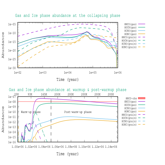
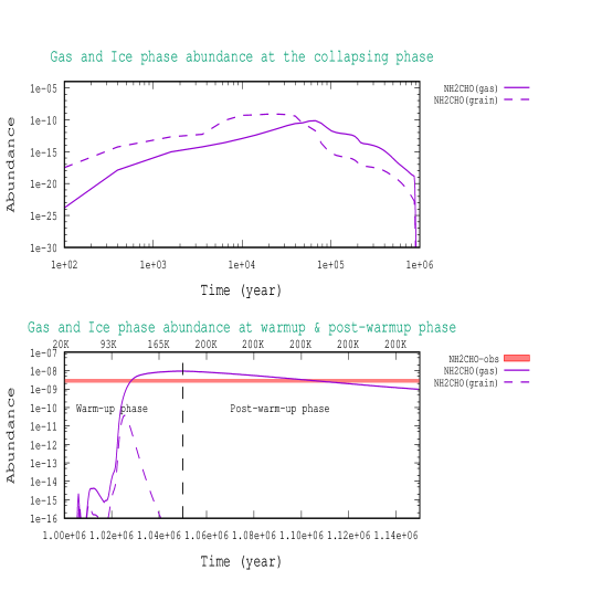
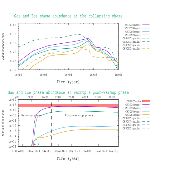
Figure 7: Chemical evolution of the three peptide bond related molecules (HNCO, NH₂CHO, CH₃NCO) and their isomers (if any). This is shown for $\rho_{max}=1.0\times 10^{7}$ cm^-3 and $T_{ice}=20$ K by considering the best-fitted parameters with Model A. Red shaded lines represent the observed abundances obtained in G10.

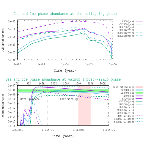
Figure 8: Chemical evolution of HNCO, CH₃NCO, and NH₂CHO during the three phases by considering the best-fit parameters of Model A. Best-fitted time zone is also highlighted. Abundance variation by avoiding Haupa et al. (2019) pathways in gas phase is also shown.

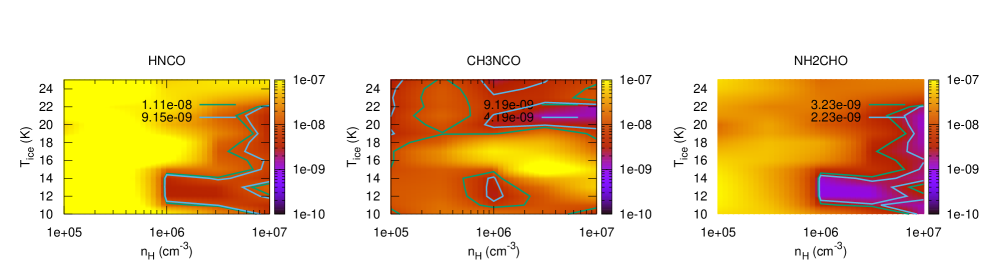
Figure 9: Parameter space obtained with Model A by considering the best-fitted parameters noted in Table 10 at an age position $1.12\times 10^{6}$ years. Color code in the right side of the each panel represents the abundance with respect to H₂.

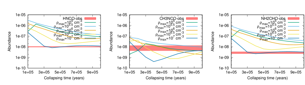
Figure 10: Abundances of HNCO, CH₃NCO, and NH₂CHO by considering different $T_{coll}$, $\rho_{max}$ with Model B.

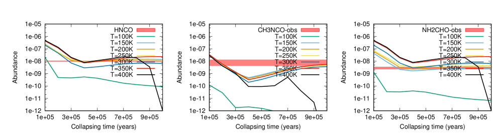
Figure 11: Abundances of HNCO, CH₃NCO, and NH₂CHO by considering $\rho_{max}=10^{7}$ cm^-3, different $T_{max}$ and $T_{coll}$ with Model B.

4.3 Modeling results

The observed abundances of HNCO, $\rm{NH_{2}CHO}$, and $\rm{CH_{3}NCO}$ are provided in Table 5. From the chemical modeling, we have seen that our obtained abundance is very much sensitive to the physical parameters ($T_{ice}$, $\rm{\rho_{max}}$, $T_{max}$, $t_{coll}$, and $t_{pw}$) and adopted rate constants. Here, we have put an extensive effort to find out the simultaneous appearance of these three nitrogen-bearing species by varying the sensitive physical parameters and rate constants of some of the key reactions. More precisely, we have prepared two models: Model A and Model B. The difference between the two models is highlighted in Table 10.

Table 10: Key differences between the Model A and Model B.

Physical parameters	Model A	Model B
${\rm{\rho_{max}}}$ ($cm^{-3}$)	$10^{7}$	$10^{5-7}$
${\rm{T_{max}}}$ (K)	200	100-400
$t_{coll}$ (years)	$10^{6}$	$10^{5-6}$
$t_{w}$ (years)	$5\times 10^{4}$	$5\times 10^{4}$
$t_{pw}$ (years)	$6.2-10\times 10^{4}$	$10^{5}$
$T_{ice}$ (K)	10-25	20
	Gas phase reactions parameterized
	Gas phase rate constants used in Model A and Model B	Rate constant used in literature
$\rm{NH_{2}+H_{2}CO\rightarrow NH_{2}CHO+H}$	$\alpha=5.00\times 10^{-12},\ \beta=-2.56,\ \gamma=4.88$	$\alpha=7.79\times 10^{-15},\ \beta=-2.56,\ \gamma=4.88$ (Skouteris et al., 2017)
$\rm{CH_{3}+HNCO\rightarrow CH_{3}NCO+H}$	$\alpha=1.0\times 10^{-12},\ \beta=0,\ \gamma=0$	$\alpha=5\times 10^{-11},\ \beta=0,\ \gamma=0$ (Quénard et al., 2018)
$\rm{H+NH_{2}CHO\rightarrow H_{2}NCO+H}$	$\alpha=1\times 10^{-10},\ \beta=0,\ \gamma=240$	$\alpha=-,\ \beta=-,\ \gamma=240-3130$ (Haupa et al., 2019)
$\rm{H+H_{2}NCO\rightarrow HNCO+H_{2}}$	$\alpha=1\times 10^{-10},\ \beta=0,\ \gamma=0$	$\alpha=-,\ \beta=-,\ \gamma=0$ (Haupa et al., 2019)
$\rm{H+H_{2}NCO\rightarrow NH_{2}CHO}$	$\alpha=1\times 10^{-10},\ \beta=0,\ \gamma=0$	$\alpha=-,\ \beta=-,\ \gamma=0$ (Haupa et al., 2019)
$\rm{H+HNCO\rightarrow H_{2}NCO}$	$\alpha=1\times 10^{-10},\ \beta=0,\ \gamma=5050$	$\alpha=-,\ \beta=-,\ \gamma=2530-5050$ (Haupa et al., 2019)

4.3.1 Results obtained with Model A

To constrain the best possible model, we have explored the parameter space around which the modeling results are in well agreement with the observational results. In this effect, we run several cases by varying the initial dust temperature ($T_{ice}$) in between $10$ to $25$ K and $\rho_{max}$ in between $10^{5}$ to $10^{7}$ cm^-3 for Model A. Since, G10 is a hot core, higher density ($10^{6}-10^{7}$ cm^-3) is preferable. It has been earlier pointed out that the G10 region is extended roughly by $0.1$ parsec and has of $\sim 10^{3}$ solar mass of matter (Cesaroni et al., 1994). From that estimation, the average density of the source is around $10^{7}$ cm^-3. It is also interesting to note that our observational analysis suggests that continuum temperatures vary within $19$ to $27$ K. Based on the observational results as a preliminary guess, we have used $\rho_{max}=10^{7}$ cm^-3 and $T_{ice}=20$ K for Model A. Initially, we have started with Model A with the rate constants of the gas phase reactions available in the literature (Skouteris et al., 2017; Quénard et al., 2018; Haupa et al., 2019). Based on some preliminary iterations of our simulation, we have varied the rate constants of the some key gas phase reactions which are controlling the abundances of the three targeted species. We have obtained a nice correlation between these three species when the rate constants listed in Table 10 is used. Quénard et al. (2018) considered the reaction between HNCO and CH₃ in the ice phase for the formation of CH₃NCO and CH₃OCN both the isomers with the same rate. However, for the gas phase formation of other isomers of CH₃NCO (CH₃CNO, CH₃OCN, CH₃ONC), Quénard et al. (2018) considered some rate coefficients of $\sim 10^{-20}$ and $5\times 10^{-11}$ cm³ s^-1. Here, instead of the rate constant $5\times 10^{-11}$ cm³ s^-1, we have considered a rate constant $10^{-12}$ cm³ s^-1 for some gas phase reactions and have used a rate $10^{-20}$ cm³ s^-1 for those reactions as it was used in Quénard et al. (2018). For the ice phase formation reactions, we kept it as it was considered by Quénard et al. (2018). To study the abundances of various isomers considered in the network, we thus choose our best fitted parameters listed in Table 10 for Model A. Time evolution of the abundances of HNCO isomers, $\rm{CH_{3}NCO}$ isomers, and $\rm{NH_{2}CHO}$ is shown in Fig. 7. Results obtained with the best fitted rate constants are shown separately in Fig. 8 for HNCO, CH₃NCO, and NH₂CHO. It clearly shows that around the age of $\sim 1.12\times 10^{6}$ years, we are having a good correlation between these three species. Parameter space obtained with the best-fitted rate constants after a suitable age position ($1.12\times 10^{6}$ years) is shown in Fig. 9. For the better understanding, abundances closer to the observed values are shown with the contours.

Among the other isomers of HNCO, HOCN is found to be significantly abundant (during the warm-up and post-warm-up phase, it has attained a peak value $4.8\times 10^{-9}$ for the best fitted parameters of Model A). This is of $\sim 10$ times lower than the lowest energy isomer, HNCO (peak abundance $4.13\times 10^{-8}$). Similarly, in between all the other isomers of $\rm{CH_{3}NCO}$, abundance of $\rm{CH_{3}OCN}$ is found to be higher. This is due to the gas phase formation of CH₃OCN by the reaction between CH₃ and HOCN. With the best-fitted parameters, we have obtained the peak abundance of $\rm{CH_{3}OCN}$ as $6.1\times 10^{-10}$ which is of $\sim 8$ times lower than that of the $\rm{CH_{3}NCO}$ (peak abundance $5.0\times 10^{-9}$). Here, we have reported the identification of HNCO and CH₃NCO in G10. However, looking at the abundances of HOCN and CH₃OCN, it should also be proposed as potential candidates for the future astronomical detection in G10. Cernicharo et al. (2016) predicted an upper limit of $6\times 10^{13}$ cm^-2 for the another isomer, CH₃CNO in Orion. Here, we have found its peak abundance $7.4\times 10^{-13}$. Converting this peak abundance in terms of the column density, we have of $\sim 10^{13}$ cm^-2 (by using a hydrogen column density $1.35\times 10^{25}$ cm^-2) which is in line with the observed upper limit.

4.3.2 Results obtained with Model B

For Model B, we did not vary any rate constants. We kept it as it was obtained with the best fitted Model A which is noted in Table 10. To find out the best-fit physical parameters for Model B, we have started with $T_{ice}=20$ K and have varied $\rho_{max}$. Figure 10 shows the variation of HNCO, CH₃NCO and NH₂CHO abundance by considering a post warm-up time ($t_{pw}$) of $10^{5}$ years. Observed abundances are also marked in each panel. We found that the abundance of these three species is highly sensitive on the chosen collapsing time scale ($t_{coll}$) and the maximum density ($\rho_{max}$) achieved during the collapsing phase. As we have increased $\rho_{max}$, abundance significantly decreased. Similarly, as we have increased $t_{coll}$, the abundances gradually decreased. Based on Figure 10, we found that $\rho_{max}=10^{7}$ cm^-3 and $T_{coll}\sim 2-3\times 10^{5}$ years are most suitable to explain the abundance of these three species simultaneously. We further have varied $T_{max}$ in between $100-400$ K by considering $\rho_{max}=10^{7}$ cm^-3. Fig. 11 shows that an increase in $T_{max}$ from $100$ K to $150$ K shows a strong increasing trend in abundance profile. We have a reasonable match when we have used $T_{max}=200$ K. In between $T_{max}=150-350$ K abundance profile shows moderate changes. Beyond $350$ K the abundances drastically decreased while we have considered a comparatively longer collapsing time scale. Thus, by considering all types of variation with Model B, we have obtained a good fit between the three targeted nitrogen-bearing species when we have used the parameters listed in Table 10. We found that our model B with $T_{coll}=(2-3)\times 10^{5}$ years, $T_{w}=5\times 10^{4}$ years and $T_{pw}=10^{5}$ years can be able to explain the observation of these three species simultaneously when we have considered $\rho_{max}=10^{7}$ cm^-3, $T_{max}=200$ K and $T_{ice}=20$ K. Obtained lower time scale with Model B is very interesting because G10 is a high-mass star forming region. Gas phase pathways required to establish the linkage between these three species are summarized in Fig. 12.

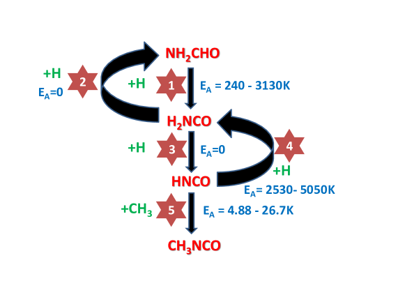
Figure 12: Chemical linkage between three nitrogen bearing molecules.

4.3.3 Chemical linkage between $\rm{HNCO}$, $\rm{NH_{2}CHO}$, and $\rm{CH_{3}NCO}$

Earlier it was proposed that HNCO and NH₂CHO are chemically linked. The successive hydrogenation reactions of HNCO was proposed for the formation of $\rm{NH_{2}CHO}$. However, the validity of the second hydrogenation reaction is ruled out by the experimental study (Noble et al., 2015). Recently a theoretical work by Haupa et al. (2019) proposed dual-cyclic hydrogen addition and abstraction reactions to support the chemical linkage between HNCO and NH₂CHO. The chemical evolution of HNCO, $\rm{NH_{2}CHO}$, and CH₃NCO with Model A are shown in Fig. 8. Gradual enhancement in the abundance of ice phase HNCO and its isomers arises because radicals become mobile enough with the increase in temperature. Beyond $80-90$ K, the diffusion time scale of the radicals become comparable to their desorption time scale and thus desorbed back to the gas phase very quickly. Also, HNCO starts to sublimate beyond $90$ K and resulting in a sharp decrease in the ice phase. The gas phase production of CH₃NCO mainly occurs by the reaction between CH₃ and HNCO. The formation rate of CH₃NCO enhances during the later phases of the simulation. In the case of $\rm{NH_{2}CHO}$, ice phase production is sufficient in the collapsing phase, but gas phase production is not adequate. In the warm-up period, a smooth transfer of $\rm{NH_{2}CHO}$ from the ice phase to the gas phase can occur. The location of this transfer depends on the adopted BE of $\rm{NH_{2}CHO}$. In the warm-up and post-warm-up phase, major portion of $\rm{NH_{2}CHO}$ is formed by the gas phase reaction between $\rm{NH_{2}}$ and $\rm{H_{2}CO}$. Due to the increased temperature, activation barrier for the hydrogen abstraction reaction of $\rm{NH_{2}CHO}$ (by reaction 16) become probable and thus produce HNCO by reaction 17 by the barrier-less reaction. To check the effects of the addition of the Haupa et al. (2019) pathways, we have checked with $\alpha=0$ for the gas phase reactions 16-19. Figure 8 shows the abundances of these three species by considering $\alpha=0$ (marked as ”NO-Haupa”). We have noticed that the abundance of gas phase HNCO is significantly affected with the inclusion of the gas phase pathways of Haupa et al. (2019). Consideration of reactions $16-19$ shows more $\rm{HNCO}$ at the end and absence of these pathways (i.e., with $\alpha=0$) reflects comparatively lower $\rm{HNCO}$. In brief, we have found that the pathways proposed by Haupa et al. (2019) are relevant for the gas phase production of HNCO around the post-warm-up period. In the first phase, $\rm{CH_{3}NCO}$ is mainly formed in the grain surface by the reaction between CH₃ and OCN. $\rm{CH_{3}NCO}$ also have formed by the reaction between $\rm{CH_{3}}$ and HNCO (Quénard et al., 2018) in the ice phase. However, it is clear from the warm-up and post-warm-up phase that the major contribution of the gas phase $\rm{CH_{3}NCO}$ is not coming from the ice phase; instead it is producing inside the gas phase itself. The gas phase formation is efficient by the HNCO channel at the warm-up and post-warm-up phase.

5 Conclusions

• We identified three molecules HNCO, NH₂CHO, and CH₃NCO in G10 which contain peptide-like bond. Earlier HNCO and $\rm{NH_{2}CHO}$ had been identified in G10, but this is the first identification of $\rm{CH_{3}NCO}$ in this source.

• We estimated the hydrogen column density of this source to be $\rm{N_{H_{2}}=1.35\times 10^{25}\ cm^{-2}}$. Our estimated optical depth is $0.136$ which suggest that the dust is optically thin. Kinetic temperatures of the gas is found to vary between $248$ to $439$ K. We estimated the column densities and fractional abundances of three observed peptide like bond containing molecules.

• From the obtained spatial distribution of these three species we speculated that they are chemically linked. Since all the transitions were marginally resolved, one need to have high angular and spatial resolution data to make a rigorous comment on their spatial distribution in G10.

• From our chemical modeling results, we also noticed that these three species are chemically linked. We found that HNCO and NH₂CHO are chemically linked by a dual-cyclic hydrogen addition and abstraction reactions proposed by Haupa et al. (2019) during the warm-up and post-warm-up phase. HNCO and CH₃NCO are also chemically related because HNCO reacts with CH₃ to form $\rm{CH_{3}NCO}$ (Fig. 12).

• Our modeling results suggest that the abundance of HOCN and $\rm{CH_{3}OCN}$ are significantly higher and could be observed in G10.

References

- Altwegg et al. (2017) Altwegg, K., Balsiger, H., Berthelier, J. J., et al. 2017, MNRAS, 469, S130
- Belloche et al. (2016) Belloche, A., Müller, H. S. P., Garrod, R. T., & Menten, K. M. 2016, Astronomy & Astrophysics, 587, A91. http://dx.doi.org/10.1051/0004-6361/201527268
- Bisschop et al. (2008) Bisschop, S. E., Jørgensen, J. K., Bourke, T. L., Bottinelli, S., & van Dishoeck, E. F. 2008, A&A, 488, 959
- Bøgelund et al. (2019) Bøgelund, E. G., McGuire, B. A., Hogerheijde, M. R., van Dishoeck, E. F., & Ligterink, N. F. W. 2019, A&A, 624, A82
- Cernicharo et al. (2016) Cernicharo, J., Kisiel, Z., Tercero, B., et al. 2016, A&A, 587, L4
- Cesaroni et al. (1994) Cesaroni, R., Churchwell, E., Hofner, P., Walmsley, C. M., & Kurtz, S. 1994, A&A, 288, 903
- Cesaroni et al. (2010) Cesaroni, R., Hofner, P., Araya, E., & Kurtz, S. 2010, A&A, 509, A50
- Chakrabarti & Chakrabarti (2000a) Chakrabarti, S., & Chakrabarti, S. K. 2000a, A&A, 354, L6
- Chakrabarti & Chakrabarti (2000b) Chakrabarti, S. K., & Chakrabarti, S. 2000b, Indian Journal of Physics Section B, 74B, 97
- Chakrabarti et al. (2015) Chakrabarti, S. K., Majumdar, L., Das, A., & Chakrabarti, S. 2015, Ap&SS, 357, 90
- Codella et al. (2017) Codella, C., Ceccarelli, C., Caselli, P., et al. 2017, A&A, 605, L3
- Cox & Pilachowski (2000) Cox, A. N., & Pilachowski, C. A. 2000, Physics Today, 53, 77
- Das et al. (2008) Das, A., Chakrabarti, S. K., Acharyya, K., & Chakrabarti, S. 2008, New A, 13, 457
- Das et al. (2019) Das, A., Gorai, P., & Chakrabarti, S. K. 2019, A&A, 628, A73
- Das et al. (2015b) Das, A., Majumdar, L., Chakrabarti, S. K., & Sahu, D. 2015b, New A, 35, 53
- Das et al. (2015a) Das, A., Majumdar, L., Sahu, D., et al. 2015a, ApJ, 808, 21
- Das et al. (2016) Das, A., Sahu, D., Majumdar, L., & Chakrabarti, S. K. 2016, MNRAS, 455, 540
- Das et al. (2018) Das, A., Sil, M., Gorai, P., Chakrabarti, S. K., & Loison, J. C. 2018, ApJS, 237, 9
- Fedoseev et al. (2015) Fedoseev, G., Ioppolo, S., Zhao, D., Lamberts, T., & Linnartz, H. 2015, MNRAS, 446, 439
- Friesen et al. (2005) Friesen, R. K., Johnstone, D., Naylor, D. A., & Davis, G. R. 2005, MNRAS, 361, 460
- Frisch et al. (2013) Frisch, M. J., Trucks, G. W., Schlegel, H. B., et al. 2013, Gaussian˜09 Revision D.01, , , gaussian Inc. Wallingford CT
- Garrod (2013) Garrod, R. T. 2013, ApJ, 765, 60
- Garrod et al. (2017) Garrod, R. T., Belloche, A., Müller, H. S. P., & Menten, K. M. 2017, A&A, 601, A48
- Gibb et al. (2003) Gibb, A. G., Wyrowski, F., & Mundy, L. G. 2003, in SFChem 2002: Chemistry as a Diagnostic of Star Formation, ed. C. L. Curry & M. Fich, 214
- Goldman et al. (2010) Goldman, N., Reed, E. J., Fried, L. E., William Kuo, I. F., & Maiti, A. 2010, Nature Chemistry, 2, 949
- Goldsmith & Langer (1999) Goldsmith, P. F., & Langer, W. D. 1999, ApJ, 517, 209
- Gorai et al. (2017a) Gorai, P., Das, A., Das, A., et al. 2017a, ApJ, 836, 70
- Gorai et al. (2017b) Gorai, P., Das, A., Majumdar, L., et al. 2017b, Molecular Astrophysics, 6, 36
- Haupa et al. (2019) Haupa, K. A., Tarczay, G., & Lee, Y.-P. 2019, J. Am. Chem. Soc., 141, 11614
- Himmel et al. (2002) Himmel, H.-J., Junker, M., & Schnöckel, H. 2002, J. Chem. Phys., 117, 3321
- Kahane et al. (2013) Kahane, C., Ceccarelli, C., Faure, A., & Caux, E. 2013, ApJ, 763, L38
- Ligterink et al. (2017) Ligterink, N. F. W., Coutens, A., Kofman, V., et al. 2017, MNRAS, 469, 2219
- López-Sepulcre et al. (2015) López-Sepulcre, A., Jaber, A. A., Mendoza, E., et al. 2015, Monthly Notices of the Royal Astronomical Society, 449, 2438
- López-Sepulcre et al. (2019) López-Sepulcre, A., Balucani, N., Ceccarelli, C., et al. 2019, ACS Earth and Space Chemistry, 3, 2122. https://doi.org/10.1021/acsearthspacechem.9b00154
- Majumdar et al. (2015) Majumdar, L., Gorai, P., Das, A., & Chakrabarti, S. K. 2015, Ap&SS, 360, 18
- Marcelino et al. (2018) Marcelino, N., Agúndez, M., Cernicharo, J., Roueff, E., & Tafalla, M. 2018, A&A, 612, L10
- Martín-Doménech et al. (2017) Martín-Doménech, R., Rivilla, V. M., Jiménez-Serra, I., et al. 2017, MNRAS, 469, 2230
- McElroy et al. (2013) McElroy, D., Walsh, C., Markwick, A. J., et al. 2013, A&A, 550, A36
- McKellar (1940) McKellar, A. 1940, PASP, 52, 187
- McMullin et al. (2007) McMullin, J. P., Waters, B., Schiebel, D., Young, W., & Golap, K. 2007, in Astronomical Society of the Pacific Conference Series, Vol. 376, Astronomical Data Analysis Software and Systems XVI, ed. R. A. Shaw, F. Hill, & D. J. Bell, 127
- Mendoza et al. (2014) Mendoza, E., Lefloch, B., López-Sepulcre, A., et al. 2014, MNRAS, 445, 151
- Motogi et al. (2019) Motogi, K., Hirota, T., Machida, M. N., et al. 2019, ApJ, 877, L25
- Müller et al. (2005) Müller, H. S. P., Schlöder, F., Stutzki, J., & Winnewisser, G. 2005, Journal of Molecular Structure, 742, 215
- Müller et al. (2001) Müller, H. S. P., Thorwirth, S., Roth, D. A., & Winnewisser, G. 2001, A&A, 370, L49
- Noble et al. (2015) Noble, J. A., Theule, P., Congiu, E., et al. 2015, A&A, 576, A91
- Ohishi et al. (2017) Ohishi, M., Suzuki, T., Hirota, T., Saito, M., & Kaifu, N. 2017, arXiv e-prints, arXiv:1708.06871
- Ossenkopf & Henning (1994) Ossenkopf, V., & Henning, T. 1994, A&A, 291, 943
- Pickett et al. (1998) Pickett, H. M., Poynter, R. L., Cohen, E. A., et al. 1998, J. Quant. Spec. Radiat. Transf., 60, 883
- Quan et al. (2010) Quan, D., Herbst, E., Osamura, Y., & Roueff, E. 2010, ApJ, 725, 2101
- Quénard et al. (2018) Quénard, D., Jiménez-Serra, I., Viti, S., Holdship, J., & Coutens, A. 2018, MNRAS, 474, 2796
- Rolffs et al. (2011) Rolffs, R., Schilke, P., Zhang, Q., & Zapata, L. 2011, A&A, 536, A33
- Ruaud et al. (2016) Ruaud, M., Wakelam, V., & Hersant, F. 2016, MNRAS, 459, 3756
- Rubin et al. (1971) Rubin, R. H., Swenson, G. W., J., Benson, R. C., Tigelaar, H. L., & Flygare, W. H. 1971, ApJ, 169, L39
- Saladino et al. (2012) Saladino, R., Botta, G., Pino, S., Costanzo, G., & Di Mauro, E. 2012, Chem Soc Rev, 41, 5526
- Sanna et al. (2014) Sanna, A., Reid, M. J., Menten, K. M., et al. 2014, ApJ, 781, 108
- Sil et al. (2018) Sil, M., Gorai, P., Das, A., et al. 2018, ApJ, 853, 139
- Sil et al. (2017) Sil, M., Gorai, P., Das, A., Sahu, D., & Chakrabarti, S. K. 2017, European Physical Journal D, 71, 45
- Skouteris et al. (2017) Skouteris, D., Vazart, F., Ceccarelli, C., et al. 2017, Monthly Notices of the Royal Astronomical Society: Letters, slx012. http://dx.doi.org/10.1093/mnrasl/slx012
- Snyder & Buhl (1972) Snyder, L. E., & Buhl, D. 1972, ApJ, 177, 619
- Song & Kästner (2016) Song, L., & Kästner, J. 2016, Physical Chemistry Chemical Physics (Incorporating Faraday Transactions), 18, 29278
- Turner (1991) Turner, B. E. 1991, ApJS, 76, 617
- Turner et al. (1999) Turner, B. E., Terzieva, R., & Herbst, E. 1999, ApJ, 518, 699
- Wakelam et al. (2017) Wakelam, V., Loison, J. C., Mereau, R., & Ruaud, M. 2017, Molecular Astrophysics, 6, 22
- Whittet (1992) Whittet, D. C. B. 1992, Journal of the British Astronomical Association, 102, 230
- Wyrowski et al. (1999) Wyrowski, F., Schilke, P., & Walmsley, C. M. 1999, A&A, 341, 882