Nonlinear extension of the quantum dynamical semigroup
Abstract
In this paper we consider deterministic nonlinear time evolutions satisfying so called convex quasi-linearity condition. Such evolutions preserve the equivalence of ensembles and therefore are free from problems with signaling. We show that if family of linear non-trace-preserving maps satisfies the semigroup property then the generated family of convex quasi-linear operations also possesses the semigroup property. Next we generalize the Gorini–Kossakowski–Sudarshan–Lindblad type equation for the considered evolution. As examples we discuss the general qubit evolution in our model as well as an extension of the Jaynes–Cummings model. We apply our formalism to spin density matrix of a charged particle moving in the electromagnetic field as well as to flavor evolution of solar neutrinos.
1 Introduction
In last decades many authors tried to generalize the standard quantum mechanical evolution. Two most important approaches are based on including nonlinear operations (see, e.g., [7, 35, 36]) and considering non-Hermitian Hamiltonians (see, e.g., [5, 28]).
Deterministic nonlinear evolutions are believed to allow for signaling [19], which was for the first time explicitly shown by Gisin in [18], compare also [29, 13]. Such evolutions are usually defined for pure states:
| (1) |
and consequently the evolution of ensembles is assumed to have the following form: If , then
| (2) |
i.e., coefficients of the ensemble do not change under the evolution. This assumption easily implies that deterministic nonlinear evolution breaks the equivalence of ensembles corresponding to the same mixed state and results in the possibility of arbitrary fast signaling [3]. In our recent paper [30] it was shown that if we replace the assumption (2) by the so called convex quasi-linearity, i.e., we allow the appropriate change of the coefficients [see Eq. (3)], then evolution satisfying such a condition preserves equivalence of ensembles and consequently such evolutions cannot be ruled out by the standard Gisin’s argument.
Let us stress that in our approach we do not change anything else in the quantum formalism but only extend admissible set of quantum evolutions by including nonlinear deterministic evolutions that do not admit superluminal signaling. This is in contrast with such nonlinear extensions of quantum mechanics that does not allow signaling but demand modifications of other quantum mechanical rules (see, e.g., [14, 22]). We also do not consider here stochastic nonlinear evolutions some of which are free from the problems with signaling and have many important applications (like in the collapse models [15, 4]).
In this paper we demonstrate that there exist a large class of convex quasi-linear evolutions. These evolutions are generated by linear non-trace-preserving quantum operations and/or derived from generalized master equation. What is interesting, recently considered evolutions generated by non-Hermitian Hamiltonians [32, 21, 10, 25] also belong to this class. It shows that convex quasi-linearity might be used as a principle joining nonlinear quantum mechanics and non-Hermitian quantum mechanics.
In Sec. 2 we remind the definition of convex quasi-linearity formulated in [30] and demonstrate that each linear non-trace-preserving quantum operation generates convex quasi-linear operation. In Sec. 3 we show that if family of linear non-trace-preserving maps satisfies the semigroup property then the generated family of convex quasi-linear operations also possesses the semigroup property. Next we consider Gorini–Kossakowski–Sudarshan–Lindblad type equation for the considered evolution. Sec. 4 is devoted to the discussion of qubit evolution in our model while in Sec. 5 we apply our formalism to two physical systems. We finish with some discussion and conclusions.
2 Admissible nonlinear quantum operations
We start with recalling the definition of convex quasi-linearity [30]. Let us denote by the convex set of density matrices. We call a map convex quasi-linear if for all and , ( ) there exist such that
| (3) |
and , . Below we show that there exists a class of convex quasi-linear operations.
An example is discussed by Kraus [26] as a generalized measurement. We considered this example in details in our previous paper [30].
Let us consider the most general linear quantum operation having the Kraus form
| (4) |
where , are Kraus operators, , is the dimension of the Hilbert space of the considered system. Furthermore, . To obtain a map into the convex set of density matrices we must normalize the in the case . Consequently, the complete quantum operation has the form
| (5) | ||||
| (6) |
i.e.,
| (7) |
Of course implies linearity of . It is easy to see that is in general convex quasi-linear, i.e.,
| (8) |
where and thus
| (9) | ||||
| (10) |
so . Of course, if then (compare [20]).
From the above definition it follows that the frequently used argument that two equivalent ensembles after nonlinear map lost this equivalence does not apply to the map . This means that can be treated as the generalized form of the acceptable quantum operation.
3 Admissible nonlinear evolutions
Now, the notion of convex quasi-linearity can be extended for deterministic time evolution. Namely, the transformation
| (11) |
is a convex quasi-linear time evolution if forms a semigroup, i.e., and the condition (3) holds for all times , i.e., for all , , there exist such that:
| (12) |
and , . In our paper [30] we have found a model of a convex quasi-linear time evolution of a qubit. Here we show that there exists a large class of natural evolutions fulfilling the above conditions.
3.1 Quasi-linear time evolution generated by linear transformations
According to the above discussion there are no formal objections to identify time evolution of density operators with a family of time dependent extended quantum operations. Consequently we postulate the evolution of the density operator in the form of the nonlinear map
| (13) |
with
| (14) |
Here , . Notice that if then the evolution is linear. The initial condition is related standardly with and for .
Let us assume that the family of linear positive maps satisfy for each , i.e., forms a one parameter semigroup. Then using linearity of and the definition of we have for each
| (15) |
i.e., . We conclude that under our assumptions the family of quantum operations forms a nonlinear realization of the one-parameter semigroup realized in the convex set of the density matrices. In particular, subfamily of trace-preserving evolutions (for ) became linear. Notice also that the above time evolution preserves convex quasi-linearity, i.e.,
| (16) |
where and
| (17) | ||||
| (18) |
and .
3.2 Nonlinear extension of the Gorini–Kossakowski–Sudarshan–Lindblad equation
The linear dynamics of an open quantum system is described by Gorini–Kossakowski–Sudarshan–Lindblad (GKSL) dynamical semigroup which is generated by the GKSL generator.
Using the infinitesimal form of the global time evolution as well as the form of the effect operator and defining , where and are Hermitian while for , , we obtain the generalization of the action of this generator to the form
| (19) |
(the detailed derivation of the above equation is given in Appendix). Notice, that the nonlinearity of the dynamics of the density operator is rather weak: It relies on the nonlinear coupling between (operator) and the -dependent trace .
From the above dynamical equation it follows that infinitesimally the operator is generated by
| (20) |
We observe that for , i.e., for , we recover the standard form of the GKSL generator:
| (21) |
Notice, that vanishing of the Lindblad generators (only is nonzero) implies that the nonlinear Kraus evolution reduces to
| (22) |
with
| (23) |
where , and we can restrict ourselves to the case of traceless generators and . Thus, the family of operators forms an one-parameter subgroup of the SL linear group. The corresponding GKSL equation reduces to the nonlinear generalization of the von Neumann equation, i.e., (compare [32])
| (24) |
with the initial condition . Let us observe that the pure states form for this evolution an invariant subset in the convex set of density operators. Indeed, we see that in this case with , so the evolution equation takes the form
| (25) |
Therefore
| (26) |
i.e., is a pure state. Therefore, we can find a counterpart of Eq. (24) for state vectors. However, the corresponding equation describing the evolution of a state vector is not uniquely determined by Eq. (24). Indeed, the whole family of equations of the form
| (27) |
where is an arbitrary real function of , leads to the evolution equation (24) for density matrices. It is worth to mention here that in general the evolution equation for a state vector also does not determine uniquely the evolution equation for density matrices.
Evolution of the form (27) for pure states with and was discussed by Gisin in [16] and subsequently with general and in [17]. Evolution similar to (24) was also considered in a specific experimental context of interaction of a two-level atom with maser photons [9]. Eq. (24) was also proposed in [10] as an evolution equation in presence of gain and loss while in [25] the information retrieval during such an evolution was discussed.
The fact that equation (24) preserves the coherence of pure states means that in the density matrix evolution this part of the master equation (19) plays different role than Lindblad operators. We will discuss this question later.
The generalized GKLS master equation (19) admits also evolutions with time-dependent generators; in particular in (24) and (27) and can be time-dependent. In such a case the global solutions have different form than those with time-independent generators. Such evolutions are very interesting because they can contain structural instability points [1].
4 Nonlinear qubit evolution
In this section we discuss qubit evolution in our model. Under the special choice of the von Neumann nonlinear equation it was also investigated recently in [32, 33, 37, 21]. In this case the initial density matrix can be taken in the following form:
| (28) |
where is a real vector satisfying the condition and is the triple of the Pauli matrices.
4.1 The case of vanishing Lindblad generators ()
The SL nonlinear evolution of in the case of vanishing of the Lindblad generators has the form
| (29) |
where the evolution matrix reads
| (30) |
with , , and g, are fixed real vectors. Moreover we assume .
This evolution can be represented on the Bloch ball as a nonlinear realization of one-parameter subgroup of the orthochronous Lorentz group homomorphic to SL. Notice that the quantities and are invariant under inner automorphisms of the SL. Therefore, values of and determine different types of evolution.
We get explicitly
| (31) |
where and for :
| (32) |
while for :
| (33) |
The general form of can be found from Eq. (29). After simple but rather lengthy calculation we obtain:
| (34) |
If we restrict our attention to the case when then and for the sake of brevity we introduce the following notation:
| (35) |
The considered case divides into three sub-classes:
(i) (), are given
in Eq. (33) and
| (36) |
(ii) , (compare Eq. (35)), , and
| (37) |
(iii) , (compare Eq. (35)), , and
| (38) |
To simplify our example, in what follow we put and , . In this case the generator satisfies the -symmetry condition and was used in [10].
Let us calculate the time evolution of the probability of finding the evolved state in eigenvectors of the Hamiltonian . For the normalized eigenvectors of the Hamiltonian have the form:
| (39) |
thus the corresponding projectors correspond to the
. We obtain:
| (40) | ||||
| (41) |
In the asymptotic limit .
| (42) | ||||
| (43) |
In the asymptotic limit .
| (44) | ||||
| (45) |
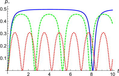
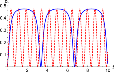
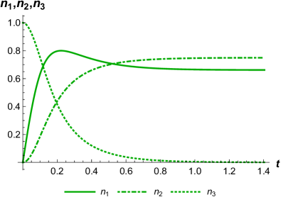
The case (when ) is the most interesting one (compare with [21]). In this case the probability of finding the evolved state in one of the eigenstates of the Hamiltonian , , is given by (45). For comparison, let us remind that the counterpart of the probability (45) obtained for the standard Rabi oscillations (i.e. in the case of evolution governed by the Hamiltonian ) has the form [12]
| (46) |
It is interesting to notice that both probabilities, (45) and (46), for fixed and attain the same maximal value equal to
| (47) |
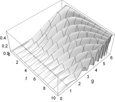
Below we illustrate the behavior of the probabilities (45) and compare it with the probabilities obtained for the standard Rabi oscillations (46). In Figs. 1 and 2 we present the probability (45) for . In Fig. 3 we compare the probability (45) with the probability obtained it the case of standard Rabi oscillations (46) (for the same values of parameters and ).
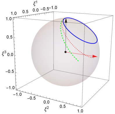
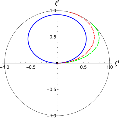
In Fig. 4 we show the trajectories of the Bloch vector under the evolution (29) with the initial condition and with and , for all three cases [Eq. (37)], [Eq. (36)], and [Eq. (38)]. Since the initial state is pure , the vector has length 1 for all . It means that the curves in Fig. 4 are situated on the Bloch sphere. For comparison, in Fig. 6 we present similar trajectories for the initial state ( and again and , ) [for calculations we used formulas (36,37,38)]. In this case the curves are inside the Bloch sphere on the plane .
Asymptotes
In this subsection we discuss asymptotic behavior of quasilinear evolutions using as a model the explicit global solution (34). Analyzing time dependence of the Bloch vector we obtain the following classes of asymptotes: (i)
| (48) |
where
| (49) |
so
| (50) |
and is the angle between and g.
(ii) and
| (51) |
(iii) and
| (52) |
(iv) In the case and the evolution is oscillatory and there are no asymptotes. It is worth to stress that almost all quasilinear evolutions (34) of qubit attain stationary states. This mean that the operator damps oscillations generated by the Hamiltonian . The only exception is the case when is perpendicular to g under condition . Notice that this damping does not increase entropy of pure initial states ( is the evolution invariant). Notice that in the neighborhood of the point given by the conditions and the character of the evolution changes drastically. It means that this point can be identified with the so called point of structural instability [1]. This point is especially important in analysis of evolutions with time dependent and/or g (see Sec. 5). A physical meaning of the vectors and g depends on the physical context (see, e.g., Sec. 5).
It can be shown that in the case (i) and for the asymptotic state is very close to the Bloch vector determining one of eigenstates of the Hamiltonian , i.e., the state of the system approaches to a stationary state. In particular, for and g parallel or anti-parallel and the asymptotic state is exactly the stationary state and it does not depend on the initial state .
4.2 The case of time-dependent g
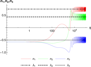
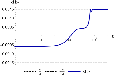
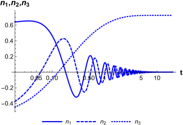
Let us consider an example of a qubit evolution governed by the nonlinear von Neumann equation (27) in the case of the time-dependence of the vector g. Let the vectors and g are oriented in the polar coordinates by the angles (, ) and (, ), respectively, so the angle between and g is about of . We choose , (inverted Morse potential), and . In that case Bloch vectors of stationary states of the Hamiltonian have the form . Furthermore, the time coordinate of the structural instability point is determined by the condition so its value is in this case. In Fig. 7 we presented the evolution of a qubit for the above parameters under initial condition . We observe a strong damping of oscillations before the instability point and a rapid conversion to an weakly oscillatory state after this time. As we see, the averages of the components of the Bloch vector n for this outgoing state are very closed to components of , represented by the dashed, dotted, dashed-dotted lines because for . Next, in Fig. 7 we present time-dependence of the average energy. We see that the energy flow is in this case directed to the qubit system. However, if we invert the direction of the vector g the average energy at the beginning goes up but next goes down to the lowest value . Thus we cannot identify the interaction of the system with the environment as dissipative.
4.3 The case with nonzero Lindblad operators
Finally, we will discuss an example with nonzero Lindblad operators. For simplicity let us assume that only one of them is nonzero, i.e., , for . In this case the nonlinear GKSL equation takes the form
| (53) |
Now, we consider an example of the Kraus form of the qubit evolution with the following choice of generators:
| (54) |
with the initial condition given in Eq. (28). The nonlinear GKSL equation implies in this case that
| (55) | ||||
| (56) |
where . Taking into account the initial condition and integrating the system we finally get
| (57a) | ||||
| (57b) | ||||
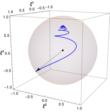
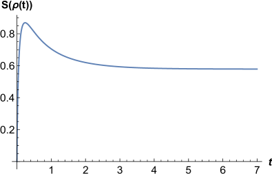
where . Notice that implies . Moreover, for : , so we obtain the pure state while for : , so we get in general the mixed state. In Fig. 8 we present an exemplary evolution of a Bloch vector in this case. In Fig. 9 we present the behavior of the von Neumann entropy under the evolution (57), we take the same initial condition and parameters as in Fig. 8.
We can also find an explicit form of Kraus operators in this case. We have
| (58) |
and
| (59) |
Furthermore
| (60) |
so we arrive at the same form of as the result of the solution of the nonlinear GKSL equation.
4.4 The Jaynes–Cummings model
In this section we show that the standard Jaynes–Cummings model [24, 34] describing the interaction of a two-level atom with a single mode of the electromagnetic (EM) field can be also generalized along the lines discussed in the paper. The standard Jaynes–Cummings Hamiltonian describing the system atom + EM field has the form
| (61) |
The creation and annihilation operators , fulfill the standard bosonic commutation relation.
In order to obtain a nonlinear generalization we replace with
| (62) |
Let us notice that subspaces
| (63) |
are invariant under the action of both and . Therefore, can be written as the following direct sum:
| (64) |
where
| (65) |
Furthermore, assuming that the initial full density matrix can be written in a similar way
| (66) |
where the conditions , imply that . Now, according to Eq. (22), during the evolution governed by (64) the density matrix (66) evolves to
| (67) |
where
| (68) | ||||
| (69) |
Notice that choosing , for we obtain the model considered in the subsection 4.1. From Eqs. (67–68) it follows that in each subspace the time evolution generator has the form (65), i.e., the corresponding vectors and are of the form and so . Thus, according to Eqs. (51–52) if the oscillations are damped and in each subspace states evolve to appropriate stationary states. However, if then for lower satisfying the states are oscillating but for are evolving to stationary states.
5 Applications
In this section we present two applications of quasi-linear evolutions: relativistic Dirac qubit in electromagnetic field and evolution of the flavor state of solar neutrinos propagating through Sun in their way to Earth. In both cases we utilize the nonlinear differential evolution equation (24) generalizing the von Neumann equation. In the former case we assume time independence of the evolution generators so we can use the global solution (34). In the latter case generators must be time(distant)-dependent which causes more sophisticated and interesting dynamics but solutions are usually achievable with use of numerical calculations only.
5.1 Evolution of the relativistic qubit carrying by a Dirac particle in electromagnetic field
Let us consider an evolution of a spin quantum charged particle (e.g. electron) which motion is generated by the electromagnetic tensor . We assume that state of the particle is determined by its four-momentum and the spin density matrix heaving in the spin basis standard form , where is the particle polarization vector, so . For a sharp momentum particle it is possible to find this matrix in the manifestly Lorentz-covariant spinorial basis [11]
| (70) |
and is known in the literature [6] as the covariant spin density matrix for a Dirac particle. Here are the gamma matrices while is the counterpart of the Pauli-Lubanski four-vector, called polarization pseudo-vector. It is defined by the relations , [8]. Notice, that can be expressed by and :
| (71) |
The four-vectors and are Minkowski-orthogonal, i.e., . Moreover , . Under the bi-spinor representation of the Lorentz group transforms according to
| (72) |
with and . In the following we will use the Weyl representation of the gamma matrices (see Appendix B). It is easy to prove that is Hermitian, non-negative definite and as well as it is related to the matrix by the formulas
| (73) | ||||
| (74) |
where satisfies the Dirac equation and intertwines spinorial and spin bases; its explicit form in the Weyl representation is given in Appendix B.
Now, we define the evolution of , satisfying the nonlinear von Neumann equation (24), by choosing its generator as follows
| (75) |
where is the Bohr magneton for a particle with charge . The complex vector
| (76) |
is known as the Riemann-Silberstein vector related to a self-dual tensor while E, B are the electric and magnetic fields, respectively. Note that
| (77) | ||||
| (78) |
so coincides with the Hamiltonian (divided by ) twisting the spin and in the case of a constant B.
Assuming that the electromagnetic field is time independent we obtain the result of integration of the von Neumann equation in the form (22). More specifically, the evolution operator takes the form
| (79) |
where we choose the proper time as the dynamical parameter to guarantee the Lorentz covariance of our formalism. Taking into account that , and choosing the rest frame values of the four-momentum and the polarization pseudo-vector as the initial conditions, i.e., so , we obtain that
| (80) |
and
| (81) |
while as well as can be calculated by means of the following equations
| (82) | ||||
| (83) |
The solution of (81) is given in (34) under appropriate identification of F and with , g, and n. On the other hand, from (79) with use of the explicit form of the gamma matrices in the Weyl form (Appendix B) we see that Eqs. (82-83) imply the following differential equations for the four-momentum and the polarization four-vector :
| (84) | ||||
| (85) |
Equation (84) is the well known covariant form of the classical charged particle momentum evolution under action of the Lorentz force and its energy change [23] while Eq. (85) is equivalent to the evolution equation for the classical pseudo-spin vector of a particle with the gyromagnetic ratio value equal to 2 (Bargmann-Michel-Telegdi (BMT) equation [2]). Summarizing, we demonstrated the semi-quantum analog of the BMT formalism where space-time coordinates are treated classically. Here the spin state is quantum. Indeed, heaving and we have determined the density matrix so we are able to calculate probabilities of measurements and evolution of averages of relativistic observables for the Dirac particle being the carrier particle of the relativistic qubit. We demonstrate evolution of the spin state of electron moving in the constant electromagnetic field in Fig 10. Notice, that this state evolves to the state which is very close to stationary state of the Hamiltonian . The exact stationary states of are achieved for parallel (antiparallel) configurations of E and B.
5.2 Evolution of the flavor quantum state of solar neutrino
As is well known, neutrino oscillates in the leptonic flavor space (space of fractional leptonic charges), i.e., it evolves between electric muonic and taonic neutrino flavors. However, neutrinos produced in the core of Sun undergo interaction with the dense solar electron plasma and, as consequence, their flavor oscillations are modified when neutrinos propagate through the Sun in their way to detectors on Earth. This is known as the Mikheyev-Smirnov-Wolfenstein (MSW) mechanism based on the Wolfenstein equation and form of the solar electron density function [27]. This process is dominated by the electron and muon neutrinos. Therefore, the effective Hamiltonian in the flavor space of electronic and muonic neutrinos is of the form
| (86) |
Here is the neutrino energy given in GeV, rad is the mixing angle between mass 1 and 2 Bloch vectors for eigenstates and , eV2,
| (87) |
(where Sun radius km) approximates the effective potential (given in neV) generated by the solar electron plasma density and is the radial distance from the center of Sun given in kilometers; is the Fermi constant while is the conversion factor. The Wolfenstein equation is simply the Schrödinger equation with time replaced by , i.e., it describes evolution of the neutrino flavor state in the neutrino travel from center of Sun to Earth.
In the paper [31] one demonstrates another point of view to this problem suggesting that the change of the neutrino state inside of the dense matter of Sun can be forced by a sort of damping of the neutrino flavor oscillations and the full evolution generator should be of the form with
| (88) |
and while the evolution equation have the form of the quasi-linear Schrödinger equation (27):
| (89) |
where
| (90) |
and , denotes the electronic and muonic flavor states, respectively.
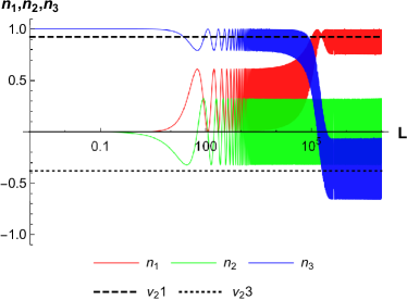
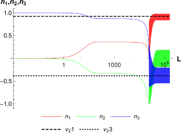
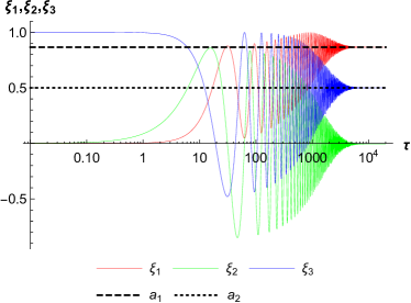
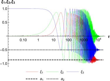
In Fig. 11 we compare both evolutions, standard MSW (, ) in Fig. 11 and generated by g (, ) in Fig. 11 for typical 10 MeV energy neutrino flux. Both approaches give the same probabilities of registration of electronic (muonic) neutrinos on Earth measured, e.g., in Super-Kamiokande detector or Sudbury Neutrino Observatory. However, it is very interesting that in the latter case, the resonant-like conversion to the final state holds in the neighborhood of the point of the structural instability of the evolution where infinitesimal change of any of the parameters changes drastically the character of the evolution [1]. In the considered case it holds for g perpendicular to in the point of the trajectory where , i.e., when so km (see Fig. 11). Before this point we observe the strong flavor oscillation damping while after conversion the neutrino state stabilizes as oscillations close to the Bloch vector of mass neutrino stationary state. In contrast, the MSW model does not show any significant disappearance of oscillations also in neighborhood of MSW critical (resonant) point km identified by the condition . An exhaustive discussion of the above questions together with experimental implications is given in the paper prepared for publication [31].
6 Discussion and conclusions
In this paper we have discussed a generalization of the notion of the quantum operations and the quantum time evolution. The generalization depends on extending the linearity of quantum operations to the quasi-linearity condition. This condition is motivated by the appearance of such operations in a “hidden” form (e.g. selective measurement [26]) in quantum formalism. On the other hand, convex quasi-linearity guarantees absence of superluminal communication. We have identified a natural class of operations satisfying this condition. Moreover, we have generalized the GKSL master equation for quasi-linear evolutions. As an example we have considered nonlinear qubit evolution. It is worth to stress that some of these qubit evolutions were discussed independently in the different context of non-Hermitian quantum mechanics [10, 32, 21]. We also discussed an appropriate modification of the Jaynes–Cummings model [24, 34] describing the interaction of a two-level atom with a single mode of the electromagnetic field. In general, the nonlinear time development of qubit is related to an interaction of the quantum system with an environment. Depending on the interrelation with environment the evolution of qubit can demonstrate different time dependence but mostly it can be interpreted as a damping of oscillations together with gain and loss of energy (Sec. 4.2). This is especially evident in presented physical applications of the introduced formalism: evolution of spin of a relativistic Dirac particle in external electromagnetic field and evolution of the flavor state of solar neutrinos propagating through the Sun. In both cases we observe damping of oscillations of the state and its asymptotic evolution to a stationary state. Moreover, the later case offers a new physical interpretation of the process of transmutation of neutrinos belonging to different flavor generations inside Sun.
To avoid misinterpretations of the introduced formalism we stress that the generator in the master equation (19) describes, similarly as the Lindblad generators, influence of an environment on a quantum system governed on the free level by the Hamiltonian . This means that the appearing in global solutions (23), (30) of the nonlinear von Neumann equation (24) or in the nonlinear Schrödinger equation (27) is the evolution generator, however, in general, it cannot be interpreted as a non-Hermitian -symmetric Hamiltonian. Notice, that the spectrum of is in general complex while -symmetric Hamiltonians have real spectra, i.e., -symmetric Hamiltonians form a subset of the considered set of generators while the corresponding trace-preserving, -symmetric evolutions belong to the introduced by us class of quasi-linear, so admissible, evolutions. This fact supports their physical acceptance because it shows that they do not lead to arbitrary fast communication.
Let us stress here that our goal was to introduce nonlinear evolution with minimal changes in the rest of quantum formalism. In our approach we do not change Born rule or projection postulate as it takes place in other nonlinear extensions of quantum mechanics ([14, 22]). But of course nonlinearity of evolution equations has implications—the superposition principle is broken during the nonlinear evolution.
Appendix A Derivation of Eq. (19)
To derive the infinitesimal form of the global time evolution (13) we proceed as follows: First, we put
| (91) |
where . On the other hand, using the composition law of the map we obtain
| (92) |
Next, with the help of the global form (13) we get
| (93) |
The initial condition implies
| (94) |
Next, we expect that in the expansion of the sum the first correction is of the order . Therefore, we put
| (95) |
where and are linear operators. Now, the nominator of Eq. (93) takes the form
| (96) |
Using this equation we obtain
| (97) |
Next, with the help of the expansion , the inverse of the denominator of Eq. (93) takes the form
| (98) |
Now, multiplying the right hand side of Eq. (96) with Eq. (98), leaving the terms of order up to , inserting , and equating the result with (91) we obtain equation (19).
Appendix B Gamma matrices and other formulas
Weyl representation of the gamma matrices
| (99) |
The explicit form of is the following:
| (100) |
moreover, it holds
| (101) |
References
- Arnol’d et al. [1994] V. I. Arnol’d, V. S. Afrajmovich, Yu. S. Il’yashenko, and L. P. Shil’niov. Bifurcation Theory, volume 5. Springer-Verlag, Berlin-Heidelberg, 1994. doi: 10.1007/978-3-642-57884-7.
- Bargmann et al. [1959] V. Bargmann, L. Michel, and V. L. Telegdi. Precession of the polarization of particles moving in a homogeneous electromagnetic field. Phys. Rev. Lett., 2:435–436, 1959. doi: 10.1103/PhysRevLett.2.435.
- Bassi and Hejazi [2015] A. Bassi and K. Hejazi. No-faster-than-light-signaling implies linear evolution. A re-derivation. European J. Phys., 36:055027, 2015. doi: 10.1088/0143-0807/36/5/055027.
- Bassi et al. [2013] A. Bassi, K. Lochan, S. Satin, T. P. Singh, and H. Ulbricht. Models of wave-function collapse, underlying theories, and experimental tests. Rev. Mod. Phys., 85:471–527, 2013. doi: 10.1103/RevModPhys.85.471.
- Bender [2007] C. M. Bender. Making sense of non-Hermitian Hamiltonians. Rep. Prog. Phys., 70:947–1018, 2007. doi: 10.1088/0034-4885/70/6/r03.
- Berestetzki et al. [1968] W. B. Berestetzki, E. M. Lifschitz, and L. P. Pitajewski. Relativistic Quantum Theory, volume 1. Nauka, Moscow, 1968.
- Białynicki-Birula and Mycielski [1976] I. Białynicki-Birula and J. Mycielski. Nonlinear wave mechanics. Ann. Phys. (New York), 100:62, 1976. doi: 10.1016/0003-4916(76)90057-9.
- Bogolubov et al. [1975] N. N. Bogolubov, A. A. Logunov, and I. T. Todorov. Introduction to Axiomatic Quantum Field Theory. W. A. Benjamin, Reading, Mass., 1975.
- Briegel et al. [1994] H.-J. Briegel, B.-G. Englert, N. Sterpi, and H. Walther. One-atom master: Statistics of detector clicks. Phys. Rev. A, 49:2962–2985, 1994. doi: 10.1103/PhysRevA.49.2962.
- Brody and Graefe [2012] D. C. Brody and E.-M. Graefe. Mixed-state evolution in the presence of gain and loss. Phys. Rev. Lett., 109:230405, 2012. doi: 10.1103/PhysRevLett.109.230405.
- Caban and Rembieliński [2005] P. Caban and J. Rembieliński. Lorentz-covariant reduced spin density matrix and Einstein–Podolsky–Rosen–Bohm correlations. Phys. Rev. A, 72:012103, 2005. doi: 10.1103/PhysRevA.72.012103.
- Cohen-Tannoudji et al. [1991] C. Cohen-Tannoudji, B. Diu, and F. Laloë. Quantum mechanics. Wiley-VCH, 1991.
- Czachor [1991] M. Czachor. Mobility and non-separability. Found. Phys. Lett., 4:351–361, 1991. doi: 10.1007/BF00665894.
- Czachor and Doebner [2002] M. Czachor and H.-D. Doebner. Correlation experiments in nonlinear quantum mechanics. Phys. Lett. A, 301:139–152, 2002. doi: 10.1016/S0375-9601(02)00959-3.
- Ghirardi et al. [1986] G. C. Ghirardi, A. Rimini, and T. Weber. Unified dynamics for microscopic and macroscopic systems. Phys. Rev. D, 34:470–491, 1986. doi: 10.1103/PhysRevD.34.470.
- Gisin [1981] N. Gisin. A simple nonlinear dissipative quantum evolution equation. J. Phys. A: Math. Gen., 14:2259–2267, 1981. doi: 10.1088/0305-4470/14/9/021.
- Gisin [1983] N. Gisin. Irreversible quantum dynamics and the Hilbert space structure of quantum kinematics. J. Math. Phys., 24:1779, 1983. doi: 10.1063/1.525895.
- Gisin [1990] N. Gisin. Weinberg’s non-linear quantum mechanics and supraluminal communications. Phys. Lett. A, 143:1–2, 1990. doi: 10.1016/0375-9601(90)90786-N.
- Gisin and Rigo [1995] N. Gisin and M. Rigo. Relevant and irrelevant nonlinear Schrödinger equations. J. Phys. A: Math. Gen., 28:7375–7390, 1995. doi: 10.1088/0305-4470/28/24/030.
- Grabowski et al. [2006] J. Grabowski, M. Kuś, and G. Marmo. Symmetries, group actions, and entanglement. Open Systems and Information Dynamics, 13:343–362, 2006. doi: 10.1007/s11080-006-9013-3.
- Grimaudo et al. [2018] R. Grimaudo, A. S. M. de Castro, M. Kuś, and A. Messina. Exactly solvable time-dependent pseudo-Hermitian su(1,1) Hamiltonian models. Phys. Rev. A, 98:033835, 2018. doi: 10.1103/PhysRevA.98.033835.
- Helou and Chen [2017] B. Helou and Y. Chen. Extensions of Born’s rule to non-linear quantum mechanics, some of which do not imply superluminal communication. Journal of Physics: Conference Series, 880:012021, 2017. doi: 10.1088/1742-6596/880/1/012021.
- Jackson [1999] John D. Jackson. Classical electrodynamics. John Wiley & Sons, New York, 1999.
- Jaynes and Cummings [1963] E. T. Jaynes and F. W. Cummings. Comparison of quantum and semiclassical radiation theories with application to the beam maser. Proc. IEEE, 51:89, 1963. doi: 10.1109/PROC.1963.1664.
- Kawabata et al. [2017] K. Kawabata, Y. Ashida, and M. Ueda. Information retrieval and criticality in parity-time-symmetric systems. Phys. Rev. Lett., 119:190401, 2017. doi: 10.1103/PhysRevLett.119.190401.
- Kraus [1983] K. Kraus. States, Effects, and Operations. Springer, Berlin, Heidelberg, 1983. doi: 10.1007/3-540-12732-1.
- Maltoni and Smirnov [2016] M. Maltoni and A. Yu. Smirnov. Solar neutrinos and neutrino physics. Eur. Phys. J. A, 52:87, 2016. doi: 10.1140/epja/i2016-16087-0.
- Moiseyev [2011] N. Moiseyev. Non-Hermitian quantum mechanics. Cambridge University Press, Cambridge, UK, 2011. doi: 10.1017/CBO9780511976186.
- Polchinski [1991] J. Polchinski. Weinberg’s nonlinear quantum mechanics and the Einstein-Podolsky-Rosen paradox. Phys. Rev. Lett., 66:397–400, 1991. doi: 10.1103/PhysRevLett.66.397.
- Rembieliński and Caban [2020] J. Rembieliński and P. Caban. Nonlinear evolution and signaling. Phys. Rev. Research, 2:012027, 2020. doi: 10.1103/PhysRevResearch.2.012027.
- [31] J. Rembieliński and J. Ciborowski. in preparation.
- Sergi and Zloshchastiev [2013] A. Sergi and K. G. Zloshchastiev. Non-Hermitian quantum dynamics of a two-level system and models of dissipative environments. Int. J. Mod. Phys. B, 27:1350163, 2013. doi: 10.1142/S0217979213501634.
- Sergi and Zloshchastiev [2015] A. Sergi and K. G. Zloshchastiev. Time correlation functions for non-Hermitian quantum systems. Phys. Rev. A, 91:062108, 2015. doi: 10.1103/PhysRevA.91.062108.
- Shore and Knight [1993] B. W. Shore and P. L. Knight. The Jaynes–Cummings model. J. Modern Optics, 40:1195–1238, 1993. doi: 10.1080/09500349314551321.
- Weinberg [1989a] S. Weinberg. Testing quantum mechanics. Ann. Phys. (New York), 194:336–386, 1989a. doi: https://doi.org/10.1016/0003-4916(89)90276-5.
- Weinberg [1989b] S. Weinberg. Precision tests of quantum mechanics. Phys. Rev. Lett., 62:485–488, 1989b. doi: 10.1103/PhysRevLett.62.485.
- Zloshchastiev [2015] K. G. Zloshchastiev. Non-Hermitian Hamiltonians and stability of pure states. Eur. Phys. J. D, 69:253, 2015. doi: 10.1140/epjd/e2015-60384-0.