Deterministic reversible model of non-equilibrium phase transitions and stochastic counterpart

Abstract

$N$ point particles move within a billiard table made of two circular cavities connected by a straight channel. The usual billiard dynamics is modified so that it remains deterministic, phase space volumes preserving and time reversal invariant. Particles move in straight lines and are elastically reflected at the boundary of the table, as usual, but those in a channel that are moving away from a cavity invert their motion (rebound), if their number exceeds a given threshold $T$. When the geometrical parameters of the billiard table are fixed, this mechanism gives rise to non–equilibrium phase transitions in the large $N$ limit: letting $T/N$ decrease, the homogeneous particle distribution abruptly turns into a stationary inhomogeneous one. The equivalence with a modified Ehrenfest two urn model, motivated by the ergodicity of the billiard with no rebound, allows us to obtain analytical results that accurately describe the numerical billiard simulation results. Thus, a stochastic exactly solvable model that exhibits non-equilibrium phase transitions is also introduced.

Pacs: 64.60.Bd, 68.03.$-$g, 64.75.$-$g; alternatives 05.45.-a, 05.70.Fh

Keywords: Billiards; Ehrenfest urn model; Non–equilibrium states; Phase transitions.

1 Introduction

Phase transitions among equilibrium states are widely investigated and well understood phenomena, which is one of the major achievements of statistical mechanics [1, 2]. Non-equilibrium phase transition [3, 4, 5, 6, 7, 8, 9], on the other hand, are much less investigated and currently, a comprehensive framework seems to be lacking, as it is in general the case for non-equilibrium statistical mechanics [10]. However, the past three decades have witnessed important advances, based on the generalization of equilibrium fluctuations theory and its consequences, such as the fluctuation-dissipation theorem and response theory [12, 11, 14, 13]. While stochastic models have occupied the largest fraction of the recent specialized literature, because simpler to treat and more inclined to produce results [15], major achievements came from the study of deterministic time reversal invariant (TRI) dynamical and dissipative, i.e. phase space volumes contracting, systems, such as those of non-equilibrium molecular dynamics (NEMD). These advances include relations between dynamical quantities such as the Lyapunov exponents and macroscopic properties such as the transport coefficients [16], fluctuation relations [17], linear response relations for perturbations of non-equilibrium steady states [18, 19, 20], and exact response relations together with novel ergodic notions [21, 22, 23]. It is indeed more natural to investigate in deterministic reversible dynamics, rather than in stochastic processes, the properties related to microscopic reversibility. In fact, stochastic processes are intrinsically irreversible, although they may enjoy the property known as detailed balance [24].

Concerning non-equilibrium phase transition, most results are obtained for stochastic processes. In fact, various kinds of abrupt transitions have been reported also in the NEMD literature. They have been observed in systems of small numbers of particles, when dissipation is increased; see, e.g. “string phases” in shearing fluids, where dissipation can be so strong that chaos of fluid particles is damped and ordered phases arise [12, 25]. The non-equilibrium Lorentz and Ehrenfest gases are even more striking from this point of view, because chaos in the dynamics of non–interacting particles can be tamed by dissipation, and an impressive variety of bifurcation–like and hysteresis–like phenomena may result, cf. [26, 27, 28, 29]. However, these behaviors have not been investigated as transitions that occur in some kind of macroscopic limit, or for conservative dynamics. Therefore, the question arises whether they can be obtained in deterministic, TRI and possibly non–dissipative systems.

In the present paper, we investigate the onset of non-equilibrium phase transitions in a conservative, TRI dynamical system of phase space $\cal M$, consisting of $N$ point particles moving in straight lines at constant speed $v=1$, within a billiard table $\Lambda$ made of two circular urns of radius $r$, connected by a rectangular channel of width $w$ and length $\ell$, cf. Fig.1.1. The channel is then divided in two parts: its left half $G_{\textup{L}}$ and its right half $G_{\textup{R}}$, each of length $\ell/2$, called gates. When particles hit the boundary $\partial\Lambda$ of the table, they are elastically reflected. This means that their speed is preserved while their velocity is reversed so that the outgoing angle with respect to the normal to $\partial\Lambda$ at the collision point equals the incoming angle.

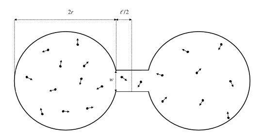
Figure 1.1: Schematic representation of the model.

So far, we have described a standard ergodic billiard [30, 31]. We then add one further dynamical rule: when the total number of particles in any of the two gates that point towards the other gate exceeds the threshold value $T$, the horizontal component of the velocity of those particles is reversed. When such a bounce–back mechanism takes place, the particles in the interested gate directed towards the other gate go back to the urn from which they came. The particles that are coming from the other urn continue unaltered their motion.

As initial condition, a certain fraction of particles is placed in the left urn and the remaining fraction in the right one; their positions and directions of velocities are chosen at random with uniform probability.

If $T\geq N$, one has the usual TRI and ergodic billiard dynamics. Ergodicity implies that each particle spends an equal amount of time in the two urns, hence, for large $N$, an equilibrium distribution of particles is reached, in the sense that approximately the same number of particles are found in the urns, apart from small oscillations about that number, and apart from very rare large deviations related to correspondingly long recurrence times. Time reversal invariance means that there exists an involution $i:{\cal M}\to{\cal M}$ of the phase space in itself, that anticommutes with the time evolution $S^{t}:{\cal M}\to{\cal M}$, so that [23]:

$$S^{t}i\Gamma=iS^{-t}\Gamma\,\quad\text{for all}~{}\Gamma\in\cal M$$ (1.1)

where $t\in\mathbb{R}$ is the time, and $i^{2}$ is the identity operator on $\cal M$. For instance, denoting by q the positions of the particles, and by p their momenta, so that $\Gamma=({\bf q},{\bf p})$ is a phase in $\cal M$, the usual reversal operation is defined by $i({\bf q},{\bf p})=({\bf q},-{\bf p})$. However, various other involutions could be considered, see e.g. [32, 33].

If $T<N$, ergodicity implies that sooner or later a number of particles larger than $T$ will be found in, say, $G_{\textup{L}}$ with velocity pointing towards $G_{\textup{R}}$. At that time, the standard billiard dynamics will be interrupted, and the particles in the left gate that were going rightward will be reflected as if they had hit a rigid vertical wall: this event does not alter the reversibility of the dynamics, as the usual involution that preserves positions and inverts momenta works also in this case. Indeed, the bounce–back mechanism within a gate is like an elastic collision with a wall: the only difference is that we cannot trivially see such a wall, because it occupies a precise region $W\subset\cal M$ of the phase space, but not of the real two dimensional space. Nevertheless, $W$ exists and is identified by the condition that more particles than $T$ lie in a gate with velocity pointing towards the other gate.

The region $W$ can be considered as removed from the phase space, like the region corresponding to particles inside a scatterer of the phase space of the Lorentz gas. Analogously, the boundary of $W$ acts like the one corresponding to the surface of the Lorentz gas scatterer: particles equally preserve their energy, and their velocities are equally elastically reflected. Indeed, suppose the $G_{\textup{L}}$ contains $T$ particles moving towards $G_{\textup{R}}$, while one more particle is entering. As the number of such particles inside $G_{\textup{L}}$ turns $T+1$, their motion is inverted, and they move back to the left urn. The last particle entering $G_{\textup{L}}$ spends only a vanishing time inside that gate, while the other particles remain in $G_{\textup{L}}$ for as long as they had been, since their horizontal speed is the same before and after bouncing back. Our main result about this conservative TRI particle system, when the geometrical parameters of the billiard table are fixed, is that:

a non-equilibrium phase transition takes place, for a given $T/N$, in the large $N$ limit.

The transition consists in switching from a state in which half of the particles lies in the left half and the rest in the right half of $\Lambda$, to the state in which almost all particles lie in one of the two halves. The non-equilibrium nature of the inhomogeneous state is revealed by the fact that it rapidly relaxes to the homogeneous equilibrium state if the rebound mechanism is switched off.

The reason for the phase transition is that large $N$ and small $T/N$ make it harder for particles in the urn with higher density to reach the urn with lower density, since the bounce–back mechanism is more frequent at higher density. Therefore, particles exiting the urn with low density reach the urn with high density and remain trapped, while the difference between the densities of the left and right urns grows. Differently, when $N$ is large but $T/N$ is not small, the density in the two urns tends to equalize and to establish a homogeneous state. For sufficiently large $N$, this scenario is confirmed by our simulations of the billiard dynamics.

This phenomenon must be properly interpreted. For any finite $N$, finite recurrence times make the system explore in time many different distributions of particles, apart from those forbidden by the bounce–back rule. As $N$ grows, such fluctuations become so rare compared to any physically relevant time scale, that a given state can be legitimately taken as stationary. This phenomenon is analogous to that concerning the validity of the $H$–theorem of the kinetic theory of gases. While no real gas is made of infinitely many molecules, hence the corresponding $H$–functional in principle is not monotonic and is affected by recurrence, the Boltzmann equation and the $H$–theorem perfectly describes such systems [34, 35]. When $N$ grows, fluctuations in the monotonic behavior of $H$ become relatively smaller and the recurrence times longer, so that for a macroscopic system, deviations from the behavior predicted by the Boltzmann equation are not expected within any physically relevant time scale.

Thus, unlike rarefied gases that have a single stationary state – the equilibrium state – our system may be found in a “polarized” steady state, in which most of the particles are gathered in one urn, or in a “spread” (homogeneous) steady state, with same numbers of particles in each urn. When the geometrical parameters of the billiard table are fixed, the onset of either of the two states depends on $N$ and on $T/N$, and stationarity must be intended as in the kinetic theory of gases.

The fact that $N$ cannot exceed $T$ inside a gate produces a state with a number density that is lower in the gates than in the urns. A gate may at most host 2$T$ particles, $T$ going towards and $T$ coming from the other gate. That corresponds to a number density $4T/\ell w$, which can be arbitrarily smaller than the highest possible density in one urn, $N/\pi R^{2}$, and than the density in the urns when they are equally populated, which approximately equals $N/2\pi R^{2}$. In other words, given the table $\Lambda$ and the threshold $T\geq 1$, a sufficiently large $N$ makes the equilibrium state impossible: both the aforementioned states, i.e., the homogeneous and the polarized one, are going to be non-equilibrium steady states.

This sheds light on the relation between microscopic reversibility and phase space volume preserving property of our dynamics, and the realization of non-equilibrium steady states and phase transitions. Indeed, our case seems to be different from those reported in the existing literature. In the first place, note that the effects of microscopic reversibility may be verified in certain phenomena, even if the standard time reversal symmetry does not hold, because alternative equivalent symmetries do, cf. e.g. [32, 33]. Such an equivalence depends on the observables of interest and on the relevance of statistics. Therefore, in certain situations reversibility may even be totally absent, without affecting properties generally associated with reversibility, such as the validity of the fluctuation relations [37, 38]. In NEMD, TRI microscopic dynamics is associated with an irreversible contraction of phase space volumes, that in some cases may be quite drastic, and be accompanied by abrupt collapse of the phase volumes dimensions [25, 26, 27, 28, 29, 39, 40].

Our dynamics, on the other hand, is TRI according to the standard reversal operation, and it is also phase space volumes preserving, although it prevents equilibrium. It seems that our case is similar to the one described in Ref.[41], concerning a molecular dynamics algorithm for simulations of a shearing fluid. In that case, a kind of Maxwell demon exchanges some fast and slow particles. When a Maxwell demon acts, some thermodynamic rules appear to be violated but, in reality, rather energetic environments must operate, greatly dissipating, in order to produce such a “violation” consistently with thermodynamics [42]. Our bounce–back mechanism, which defeats the trend towards equilibrium of the standard billiard [30], is an analogous mechanism.

As in other cases, the statistical nature of the quantities of our interest justifies the introduction of a stochastic counterpart of our deterministic model, which allows a detailed mathematical detailed analysis not easily accessible in the deterministic framework. In general, associating stochastic processes to deterministic systems has proven quite useful; for instance, it has been the key, via representations of SRB measures, to results such as the fluctuation relation [17, 43]. Therefore, the second part of this paper is devoted to a stochastic two urn model that is inspired by the deterministic model, and for which the existence of a non-equilibrium phase transition can be investigated analytically. We remark that thresholds affecting particles dynamics have proven effective in other investigations of stochastic models such as those of Refs.[44, 45, 46]. We also observe that phase transitions are found in stochastic systems similar to ours, such as the Ehrenfest urn model with interactions [47, 48]. In fact, our stochastic model reduces to the classical Ehrenfest urn model, when the bounce–back mechanism is inhibited, and the system asymptotically relaxes to equilibrium [49].

To match the deterministic and the stochastic models, quantities such as the frequency of the bounce–back events are required. For billiard systems, these quantities can be estimated considering the ergodicity of the standard billiard, and the fact that it yields more accurate results for larger $N$. Initially, the dynamics appears like that of an ergodic billiard with a hole [31, 50]. Then, if the number of particles in one urn is large, the adjacent gate is rapidly filled with particles moving towards the other urn, which then bounce back. Therefore, the larger $N$, the less likely for particles to leak out of one urn. At the same time, motion inside the urns is chaotic, which tends to produce uniform space and velocity distributions, justifying a probabilistic approach. In Section 2, these calculations are carried out, and are shown to accurately describe the dynamics.

2 The deterministic model

This section is devoted to the study of the deterministic billiard model. A preliminary heuristic discussion will be followed by the numerical study and by some analytical interpretations of the results.

2.1 Polarized and homogeneous states. Outlet and leaking currents

The motion of particles inside each reservoir is ergodic, therefore, for large $N$, we expect that particles leave an urn to enter the adjacent gate with a rate that simply depends on $N$, on the radius of the urn, on the width of the gate and on the speed of the particles. If the rate is low, a given threshold $T$ may not be exceeded by the number of particles in the gate, and particles safely cross the channel towards the opposite urn. On the other hand, if such a rate is high with respect to the typical time needed by particles to walk through the gates, $T$ can be frequently exceeded, making particles bounce back.

Starting from a configuration in which the two reservoirs share the same (large) number of particles, we have two extreme situations to consider for stationary states:

i) If the ratio $T/N$ is large, the bounce–back mechanism is not effective. Particles move freely from one reservoir to the other and, at stationarity, the number of particles in the two urns is approximately constant and equal. This state is stable and will be referred to as a homogeneous state. In this case, relatively large average currents flowing in opposite directions from one urn to the other, that we call outlet currents, balance each other.

ii) If the ratio $T/N$ is small, the particles inside a gate may frequently exceed $T$ and bounce back to their original urn. The corresponding average currents, which we call leak currents, are small, hence the initial condition with an equal number of particles in the two urns is only slightly perturbed by them. However, even a small fluctuation in this distribution of particles, due to an instantaneous unbalanced leak current, will lead to a different bounce–back frequency in the two urns, which will in turn amplify the difference in the number of particles in the two urns, till an inhomogeneous (polarized) state will be achieved.

To distinguish between the different stationary states, we introduce an order parameter $\chi$, called mass displacement, that is the absolute value of the difference between the time averaged number of particles in the two halves of the table $\Lambda$, divided by $N$. The parameter $\chi$ is thus close to one in the polarized state and close to zero in the homogeneous state. Note that in the appropriate region of the parameter space, even when starting from the homogeneous state (actually, the initial datum is irrelevant), the system ends up in the polarized state. This can be seen as an instance of a transient uphill mass transport phenomenon, in which particles are observed to preferably move from regions of lower concentration to regions of higher concentration [51, 52, 53, 54].

2.2 Efficiency of the bounce–back mechanism

Here we estimate the values of the parameters for which the bounce–back mechanism becomes effective. Thus, for a fixed total number of particles $N$, we derive Equation (2.5), which identifies, in the parameter space $r$–$w$–$\ell$–$T$, the hypersurface separating the region in which the threshold mechanism is efficient from the region in which it is not.

The idea is the following: relying on the ergodicity argument described above, and assuming very large $N$, we consider the homogeneous state and compare the rate at which particles enter a gate as well as the typical time needed to cross the gate. Take $\delta$ such that $v\delta\ll w$, recalling that $v=1$. The probability that the particle enters a gate from the adjacent urn in a time smaller than $\delta$ is $p_{\delta}=2wv^{2}\delta/(2\pi v\cdot\pi r^{2})=wv\delta/(\pi A)$ [55, Appendix A], where

$$A=A(r,w)=\pi r^{2}-r^{2}\arcsin\Big{(}\frac{w}{2r}\Big{)}+\frac{1}{4}w\sqrt{(2r)^{2}-w^{2}}$$ (2.3)

is the area of the urn. Obviously, $A\approx\pi r^{2}$ when $w$ is small compared to the radius $r$ of the urn. Requiring $p_{\delta}\sim 1$, we get $\pi A/(wv)$ as an estimate of the typical time to exit the reservoir.

The average horizontal component of the particles entering the channel is $2v/\pi$. Hence, the typical time to cross the gate is $(\ell/2)/(2v/\pi)=\ell\pi/(4v)$.

Consider the time $t$ and the small interval $\delta$. Each of the $N/2$ particles in the reservoir tries to enter the channel in the small time $\delta$. It is like performing $(N/2)(t/\delta)$ Bernoulli trials with success probability $wv\delta/(\pi A)$. Hence, the number of particles entering the channel from one of the two reservoir during the time $t$ is estimated by $t(N/2)wv/(\pi A)$. More in general, we define, for later use, the outlet current $J_{\textup{o}}(n)=nwv/(\pi A)$ coming from an urn with $n$ particles.

Since on average particles take about the time $\ell\pi/(4v)$ to cross the gate, the typical number of particles inside a gate is equal to the number of particles which enter it in the time $\ell\pi/(4v)$, namely, $\ell\pi/(4v)(N/2)wv/(\pi A)=Nw\ell/(8A)$.

We conclude that the bounce–back mechanism is efficient provided the parameters of the model satisfy the inequality

$$\frac{Nw\ell}{8A}>T\;\;.$$ (2.4)

Thus, exploiting (2.3), we expect that the region of the parameter space $r$–$w$–$\ell$–$T$ in which the threshold mechanism is efficient and that in which it is not are separated by the hypersurface

$$Nw\ell=T8\Big{[}\pi r^{2}-r^{2}\arcsin\Big{(}\frac{w}{2r}\Big{)}+\frac{1}{4}w\sqrt{(2r)^{2}-w^{2}}\Big{]}\,.$$ (2.5)

2.3 Numerical results

To support numerically this intuition, we simulated the model and measured the stationary average value of the mass displacement

$$\chi={\left|N_{R}-N_{L}\right|\over N},$$ (2.6)

where $N_{L}$ is the number of particles in the left half of $\Lambda$, and $N_{R}$ that of the particles in its right half, with $N_{L}+N_{R}=N$. In particular, a random initial condition $\Gamma\in\cal M$ is used, and the standard event–driven algorithm is implemented, recording the phase whenever a particle collides with the boundary $\partial\Lambda$, reaches the entrance of a gate or crosses from one gate to the other. This is necessary in our case, in order to verify whether the particles in a gate going towards the other gate exceed $T$, or do not.

A simulation is first performed up to a number $M_{\rm t}$ of events that are sufficient for the instantaneous value of $\chi$ to become constant (modulo fluctuations), i.e. until a stationary state appears to be reached. This requires large $N$, and we have found that $N=O(10^{3})$ suffices. The simulation stops when a total number $M_{\text{f}}$ of events is reached. Then, $\chi$ is averaged over the time corresponding to the final $M_{\text{f}}-M_{\rm t}$ steps; an ensemble of such averages is obtained simulating the evolution from different initial conditions; and finally the ensemble average of the time averages is produced.

For sake of comparison, our simulations have been collected in classes in which two parameters are fixed to some reference value, while the remaining pair of parameters varies in a relatively wide range of values. In Figure 2.2, we have thus plotted our results for $N=10^{3}$. For each value of the parameters we have considered one single realization of the dynamics, namely, the evolution of the system starting from one random initial configuration $\Gamma$ with mass spread $\chi=0.50$. The reference value for the four parameters are the following $r=1$, $T=10$, $w=0.5$, and $\ell=0.5$. The simulation has been performed with $M_{\text{t}}=5\times 10^{6}$ and $M_{\text{f}}=6\times 10^{6}$. We have performed the same simulations starting from an initial configuration with mass spread equal to $0,0.25,0.75,1$ and we found perfectly similar results.

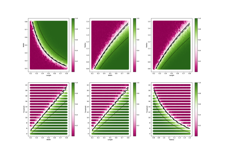
Figure 2.2: Average mass displacement $\chi$ for $N=10^{3}$, as a function of two parameters, with the remaining ones fixed to a reference value. The reference values are $r=1$, $T=10$, $w=0.5$, and $l=0.5$. The black dotted line is the theoretical curve (2.5). The black dashed dotted line is obtained by multiplying the right hand side of the theoretical curve (2.5) by the fitting parameter $0.75$. The black solid line is the curve (2.12).

The parameter region has been chosen around the curve defined by the equation (2.5) and derived in Subsection 2.2. Indeed, if all the parameters but two are fixed, (2.5) is the algebraic equation of a curve in the plane in terms of the two varying parameters. We notice that such a curve (black dotted line in the Figures 2.2) discriminates the region in which the bounce–back mechanism is efficient and that in which it is not, thus locating a rather sharp transition from polarized to homogeneous states. In our figures, the green region corresponds to a polarized state ($\chi=1$), while the deep purple region corresponds to a homogeneous state ($\chi=0$).

In all the plots, the black dotted theoretical curve lies closer to the green part of the graph, which is the inhomogeneous steady state. Hence, though the level curves of $\chi$ rather closely follow the theoretical curve, the theoretical prediction underestimates the bounce–back mechanism corresponding to finite $N$ and $w$. Indeed, according to the inequality (2.4), in the plane $\ell$–$w$ the region in which the bounce–back mechanism is efficient lies above the curve, whereas in our pictures, except one, it lies below it. As noted above, this is not a surprise, since (2.4) is not a sharp mathematical inequality, but rather an informed guess, whose accuracy should increase with $N$, as long as ergodicity can be legitimately invoked. As a matter of fact, we observe that the numerically computed interface differs from the theoretical one just by a multiplicative factor, cf. the dashed dotted black curve in Figure 2.2, which is the theoretical curve multiplied by a number.

In Figure 2.3, we have plotted our results for $N=10^{4}$. For each value of the parameters we have considered one single realization of the dynamics starting from a randomly chosen initial configuration with initial mass spread $0.50$. The reference value for the four parameters are $r=1$, $T=100$, $w=0.5$, and $\ell=0.5$. The simulation has been performed with $M_{\text{t}}=5\times 10^{6}$ and $M_{\text{f}}=6\times 10^{6}$. Results are similar to those obtained in the case with smaller values of $N$. As before, we have performed the same simulations starting from an initial configuration with values of mass spread equal to $0,0.25,0.75,1$ and we again found perfectly similar results.

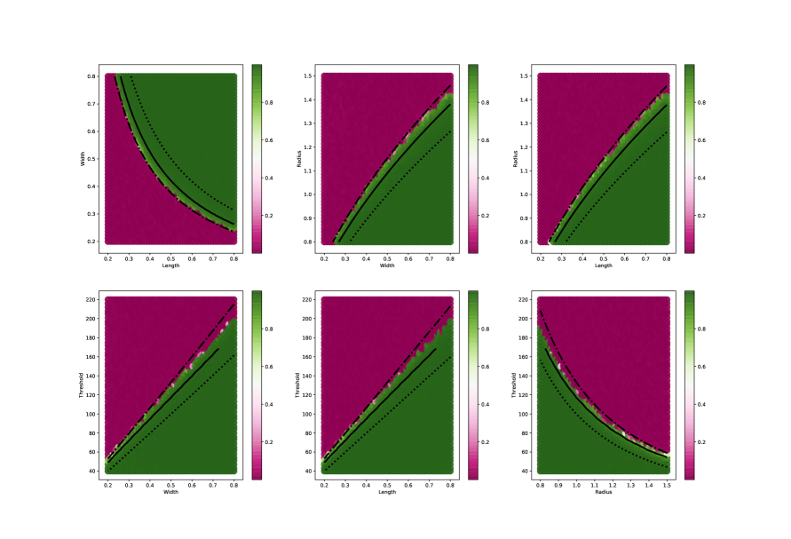
Figure 2.3: Mass displacement $\chi$ as a function of two parameters with the remaining ones fixed to their reference value. The reference values are $r=1$, $T=100$, $w=0.5$, and $\ell=0.5$. The total number of particles is $N=10^{4}$. The black dotted line is the theoretical curve (2.5). The black dashed dotted line is obtained by multiplying the right hand side of the theoretical curve (2.5) by the fitting parameter $0.75$. The black solid line is the curve (2.12).

2.4 Computing the transition line

We now develop a theoretical argument to explain the (rather) sharp transition between the polarized and the homogeneous states observed numerically in Subsection 2.3. Our main result is equation (2.12) below. This provides the hypersurface at which the transition between the polarized and the homogeneous state occurs in the parameter space $r$–$w$–$\ell$–$T$ for fixed number of particles $N$.

The key idea is to estimate the leaking current $J_{\textup{l}}(n)$ emerging from a reservoir containing $n$ particles. Consider a time interval of length $t$ and partition it in smaller intervals of length $\tau=\ell\pi/(4v)$, the typical time a particle takes to cross the gate. Moreover, partition each of such time intervals in $\tau/\delta$ very small intervals of duration $\delta$ such that $v\delta\ll w$. As remarked in Subsection 2.2, the probability that one particle in the urn enters the gate during a time interval of length $\delta$ is $p_{\delta}=wv\delta/(\pi A)$. Thus, the probability that $s$ particles enter the gate in the time interval of width $\tau$ is

$${n\tau/\delta\choose s}p_{\delta}^{s}(1-p_{\delta})^{n\tau/\delta-s}\;.$$ (2.7)

Since $p_{\delta}n\tau/\delta$ is equal to the constant $nw\ell/(4A)$, by the Poisson limit theorem, in the $\delta\to 0$ limit, the probability (2.7) tends to

$$\frac{\lambda^{s}}{s!}\,e^{-\lambda}\;\;\textup{ with }\;\;\lambda=n\frac{w\ell}{4A}\;.$$ (2.8)

Moreover, the probability that at most $T$ particles enter the gate during the time interval of width $\tau$ is

$$P_{\tau}=\sum_{s=0}^{T}\frac{\lambda^{s}}{s!}\,e^{-\lambda}=\frac{\Gamma(T+1,\lambda)}{T!}\;,$$ (2.9)

where we recall the definition of the Euler incomplete $\Gamma$ function

$$\Gamma(y,x)=\int_{x}^{\infty}t^{y-1}e^{-t}\,\textup{d}t\;\ y>0.$$ (2.10)

Thus, typically, only in $P_{\tau}t/\tau$ intervals, out of the total $t/\tau$, the particles entering the gate will not bounce back because of the threshold mechanism. The number of particles that will cross the gate can be estimated as the typical number of particles that enter the gate in an interval of length $\tau$ conditioned to the fact that such a number is smaller than $T$ multiplied times $P_{\tau}t/\tau$. Hence, the leaking current from an urn with $n$ particles is given by

$$J_{\textup{l}}(n)=\frac{1}{t}\frac{P_{\tau}t}{\tau}\frac{1}{P_{\tau}}\sum_{s=0}^{T}s\frac{\lambda^{s}}{s!}\,e^{-\lambda}=\frac{4v}{\ell\pi}\sum_{s=0}^{T}s\frac{\lambda^{s}}{s!}\,e^{-\lambda}=\frac{4v}{\ell\pi}\lambda\sum_{k=0}^{T-1}\frac{\lambda^{k}}{k!}\,e^{-\lambda}=n\frac{wv}{\pi A}\frac{\Gamma(T,\lambda)}{(T-1)!}\;,$$ (2.11)

where we used the change of variables $s-1=k$. We remark that (2.11) corresponds to a stationary average. We then conclude that the transition line between the polarized and the homogeneous state is given by the equation:

$$\frac{\textup{d}J_{\textup{l}}}{\textup{d}n}\bigg{|}_{\chi=0}=\frac{wv}{\pi A}\frac{\Gamma(T,\lambda)-\lambda^{T}e^{-\lambda}}{\Gamma(T)}\bigg{|}_{\chi=0}=0,$$ (2.12)

where we used that, for any positive integer $T$, $\Gamma(T)=(T-1)!$.

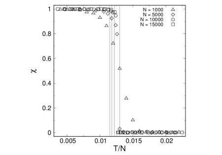
Figure 2.4: Mass displacement $\chi$ as a function of $T/N$, for growing $N$. The mass displacement for different values of $N$ has been measured following the procedure described in Section 2.3 for $r=1$, $\ell=0.5$, $w=0.5$ and $T$ and $N$ chosen as described in the picture labels. The four grey vertical lines denote the position of the transition estimated using (2.12) for $N=1.5\times 10^{4},1.0\times 10^{4},5.0\times 10^{3},1.0\times 10^{3}$ from the left to the right, respectively.

To understand the nature of the transition, let us observe Figure 2.4. As initially conjectured, it appears that this transition is determined by the growth of $T/N$, and that it is sharper at larger $N$. The transition from homogeneous to polarized steady states occurs when $T/N$ decreases and crosses a critical value that depends on the other parameters of the model, cf.  equation (2.4). Moreover, the transition is sharper if $N$ is larger. The vertical lines represent the transition value obtained from (2.12) for the different values of $N$ considered in the picture. The larger $N$, the smaller the transition value, which appears to converge to a finite number in the $N\to\infty$ limit.

2.5 Estimate of the mass displacement

In this section we derive an approximate closed implicit expression for the mass displacement in the polarized state. We proceed as follows: We consider the system in the polarized state and suppose that the right urn is the highly populated one. Consistently with our intuition, this is realized if the right urn is initially sufficiently more populated than the left urn, e.g. because a fluctuation has produced this situation. Therefore, in the following, we only consider situations in $N_{R}(0)>N_{L}(0)$, which implies $N_{R}(t)>N_{L}(t)$ for times $t>0$. Then, in the stationary state, the outlet current from the left urn equals the leak current from the right reservoir, which, recalling the definition of outlet current given in Section 2.2 and that of leaking current given in (2.11), amounts to

$$\frac{N_{\textup{L}}wv}{\pi A}=N_{\textup{R}}\frac{wv}{\pi A}\frac{\Gamma(T,\lambda_{\textup{R}})}{(T-1)!}\;,$$ (2.13)

where $\lambda_{\textup{R}}=N_{\textup{R}}w\ell/(4A)$. This leads to

$$\chi=\frac{1-\Gamma(T,\lambda_{\textup{R}})/(T-1)!}{1+\Gamma(T,\lambda_{\textup{R}})/(T-1)!},$$ (2.14)

where $\lambda_{\textup{R}}$ depends on $\chi$ via $N_{R}$.

3 The stochastic model

In the stochastic Ehrenfest urn model, $N$ balls are initially placed in two urns. At each discrete time one of the two urns is chosen with a probability proportional to the number of particles it contains and one of its particles is moved to the other urn. If we denote by $n$ the number of particles in one of the two urns, say the first, the model is a discrete time Markov chain on the state space $\{0,1,\dots,N\}$ with transition matrix $p_{n,n+1}=(N-n)/N$ and $p_{n,n-1}=n/N$.

To mimic the billiard dynamics of Section 1, we modify the Ehrenfest stochastic model introducing a threshold $T\in\{0,1,\dots,N-1\}$ that reduces the transition rates from one urn, when its number of particles exceeds $T$. More precisely, we pick $\varepsilon\in(0,1]$ and, for $T<N/2$, we set

$$p_{n,n+1}=\frac{N-n}{N}\varepsilon\;\;\textrm{ and }\;\;p_{n,n-1}=\frac{n}{N}\,,\quad\mbox{for $n\leq T$,}$$ (3.15)

$$p_{n,n+1}=\frac{N-n}{N}\varepsilon\;\;\textrm{ and }\;\;p_{n,n-1}=\frac{n}{N}\varepsilon\,,\quad\mbox{for $T<n<N-T$,}$$ (3.16)

$$p_{n,n+1}=\frac{N-n}{N}\;\;\textrm{ and }\;\;p_{n,n-1}=\frac{n}{N}\varepsilon\,,\quad\mbox{for $n\geq N-T$}.$$ (3.17)

On the other hand, for $T>N/2$, we set:

$$p_{n,n+1}=\frac{N-n}{N}\varepsilon\;\;\textrm{ and }\;\;p_{n,n-1}=\frac{n}{N}\,,\quad\mbox{for $n\leq N-T$,}$$ (3.18)

$$p_{n,n+1}=\frac{N-n}{N}\;\;\textrm{ and }\;\;p_{n,n-1}=\frac{n}{N}\,,\quad\mbox{for $N-T<n<T$,}$$ (3.19)

$$p_{n,n+1}=\frac{N-n}{N}\;\;\textrm{ and }\;\;p_{n,n-1}=\frac{n}{N}\varepsilon\,,\quad\mbox{for $n\geq T$.}$$ (3.20)

The standard stochastic Ehrenfest urn model is recovered for $\varepsilon=1$.

3.1 The stationary measure

The stationary measure for the Markov chain can be computed relying on the reversibility condition

$$\mu(n)p_{n,n+1}=\mu(n+1)p_{n+1,n}$$ (3.21)

for any $n=0,\dots,N-1$.

To compute the stationary measure we have to distinguish two cases. For $T<N/2$ the equality (3.21) can be rewritten as follows:

$$\mu(n)\varepsilon\frac{N-n}{N}=\mu(n+1)\frac{n+1}{N},\;\;n\leq T-1$$

$$\mu(T)\varepsilon\frac{N-T}{N}=\mu(T+1)\varepsilon\frac{T+1}{N}.\;\;n=T$$ (3.22)

$$\mu(n)\varepsilon\frac{N-n}{N}=\mu(n+1)\varepsilon\frac{n+1}{N},\;\;T<n\leq N-T-1$$

$$\mu(n)\frac{N-n}{N}=\mu(n+1)\varepsilon\frac{n+1}{N},\;\;n\geq N-T.$$

Solving the recurrence relations (3.1) by induction, we find the stationary measure

$$\mu(n)={\varepsilon^{n}\over Z}\left(\genfrac{}{}{0.0pt}{}{N}{n}\right),\;\;n\leq T$$

$$\mu(n)={\varepsilon^{n}\over Z}\left(\genfrac{}{}{0.0pt}{}{N}{n}\right),\;\;T+1\leq n\leq N-T$$ (3.23)

$$\mu(n)=\frac{\varepsilon^{T}}{Z\varepsilon^{n-(N-T)}}\left(\genfrac{}{}{0.0pt}{}{N}{n}\right),\;\;n\geq N-T+1,$$

where $Z$ is the normalization constant. On the other hand, for $T>N/2$, the equality (3.21) can be rewritten as follows:

$$\mu(n)\varepsilon\frac{N-n}{N}=\mu(n+1)\frac{n+1}{N},\;\;n\leq N-T-1$$

$$\mu(N-T)\varepsilon\frac{N-(N-T)}{N}=\mu(N-T+1)\frac{N-(N-T)+1}{N}.\;\;n=N-T$$ (3.24)

$$\mu(n)\frac{N-n}{N}=\mu(n+1)\frac{n+1}{N},\;\;N-T<n<T-1$$

$$\mu(n)\frac{N-n}{N}=\mu(n+1)\varepsilon\frac{n+1}{N},\;\;n\geq T-1.$$

Solving the recurrence relations (3.1) by induction, we find the stationary measure

$$\mu(n)={\varepsilon^{n}\over Z}\left(\genfrac{}{}{0.0pt}{}{N}{n}\right),\;\;n\leq N-T+1$$

$$\mu(n)={\varepsilon^{N-T+1}\over Z}\left(\genfrac{}{}{0.0pt}{}{N}{n}\right),\;\;N-T+2\leq n\leq T-1$$ (3.25)

$$\mu(n)=\frac{\varepsilon^{N-T+1}}{Z\varepsilon^{n-T+1}}\left(\genfrac{}{}{0.0pt}{}{N}{n}\right),\;\;n\geq T,$$

where $Z$ is the normalization constant.

3.2 The large $N$ behavior

We are interested in the structure of the stationary measure as $N$ is large. We set $T=\lfloor\lambda N\rfloor$ with $\lambda\in(0,1)$. We define

$$I(n)=-\frac{1}{N}\log\mu(n)$$ (3.26)

for $n=0,1,\dots,N$ and look for its minima.

We discuss in detail the case $\lambda>1/2$. In the first region, $n\leq N-T+1$, simple algebraic calculations yield

$$I(n+1)-I(n)=-\frac{1}{N}\Big{[}\log\varepsilon+\log\frac{N-n}{n+1}\Big{]}.$$ (3.27)

Since

$$I(n+1)-I(n)>0\Longleftrightarrow n>\frac{\varepsilon N-1}{1+\varepsilon},$$ (3.28)

$I(n)$ has a local minimum at $n^{\star}=\lfloor(\varepsilon N-1)/(1+\varepsilon)\rfloor$ in the region $0\leq n\leq N-T+1$ provided

$$\varepsilon N>1\;\;\textrm{ and }\;\;\varepsilon<\varepsilon^{*}=\frac{1}{\lambda}-1.$$ (3.29)

The first inequality is obvious. Concerning the second, we note that $(\varepsilon N-1)/(1+\varepsilon)<N-\lambda N+1$ is equivalent to $[\lambda(1+\varepsilon)-1]N<2+\varepsilon$, which can be satisfied for arbitrarily large $N$ only if the square bracket in the left hand side is negative.

With a similar argument we find that in the second region, $N-T+2\leq n\leq T-1$, the function $I(n)$ has a local minimum at $n^{\star\star}=\lfloor(N-1)/2\rfloor$. In the third region, $n\geq T$, results are like in the first region, taking $N-n$ in place of $n$.

Finally, we compare the values attained by the function $I(n)$ at the two local minima $n^{\star}$ and $n^{\star\star}$. Assuming $N$ to be large, so that, in particular, the approximations $n^{\star}\approx\varepsilon N/(1+\varepsilon)$ and $n^{\star\star}\approx N/2$ are valid, we get

$$I(n^{\star})-I(n^{\star\star})<0\Longleftrightarrow 2\varepsilon^{1-\lambda}<1+\varepsilon.$$ (3.30)

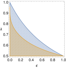
Figure 3.5: Left panel: Regions where conditions (3.30) (small bronze region) and the condition on the right in (3.29) (large blue region) are satisfied. Right panel: Regions where conditions (3.32) (small bronze region) and the condition on the right in (3.31) (large blue region) are satisfied.

As shown in the left panel of Figure 3.5, condition (3.30) is stronger than the condition on the right in equation (3.29). Hence we have the following options: if condition (3.30) is satisfied, the stationary measure concentrates, in the large $N$ limit, on the polarized state, in which $n=n^{\star}$ or $n=N-n^{\star}$ (smaller bronze region in the left panel of Figure 3.5). If the condition on the right in (3.29) is satisfied, but (3.30) is violated (part of the parameter space between the large blue and the small bronze region in the left panel of Figure 3.5), then the stationary measure concentrates, in the large $N$ limit, on the homogeneous state, in which $n=N/2$. The states with $n=n^{\star}$ or $n=N-n^{\star}$ are sort of metastable states. For different values of the parameters the measure simply concentrates on the state $n=N/2$.

For $\lambda<1/2$ the discussion is similar. In this case, conditions (3.29) and (3.30) are respectively replaced by

$$\varepsilon N>1\;\;\textrm{ and }\;\;\varepsilon<\frac{\lambda}{1-\lambda}$$ (3.31)

and

$$I(n^{\star})-I(n^{\star\star})<0\Longleftrightarrow 2\varepsilon^{\lambda}<1+\varepsilon,$$ (3.32)

see also the right panel in Figure 3.5.

3.3 Numerical simulations

In this section we report on Monte Carlo simulations meant to test the results obtained in Section 3.2 and to show the existence of a sort of metastable state, close to the transition line defined by conditions (3.30) and (3.32).

Figure 3.6: Number of particles in urn one (disks) and two (squares). Solid (open) symbols refer to the initial condition in the polarized (homogeneous) state $n=\varepsilon N/(1+\varepsilon)$ ($n=N/2$). Parameters: $N=250$, $\varepsilon=0.2$ and, in lexicographic order, $\lambda=0.05,0.31,0.45,0.52,0.69,0.95$.

In Figure 3.6 we plot the urn content as a function of time for experiments with $N=250$ and $\varepsilon=0.2$. The initial state is either polarized (solid symbols) or homogeneous (open symbols). Looking at the picture in lexicographic order, the first one refers to the case $\lambda=0.005$ so that the system is represented by a point in the bottom (white) region in the right picture of Figure 3.5. The predicted stationary state is the homogeneous one and the picture shows that with both initial conditions, the system quickly jumps to such a homogeneous state and goes on fluctuating around it at any time. In the second picture $\lambda=0.31$ and the point representing the system in the right picture of Figure 3.5 falls in the middle (blue) region, very close to the upper (orange) transition line. As confirmed by the simulation, the stationary state is still the homogeneous one, but if the initial condition is polarized, then the system spends a lot of time in such a state before performing, at a random time, an abrupt transition to the homogeneous one. In other words, in the middle (blue) region of Figure 3.5, very close to the upper (orange) transition line, the polarized state appears to be a metastable state [56, 57]. In the third picture we have $\lambda=0.45$, and the point representing the system in the right panel of Figure 3.5 falls in the upper (bronze) region. As confirmed by the simulation, the stationary state is polarized.

Figure 3.7: As in Figure 3.6 with parameters $N=1000$, $\varepsilon=0.4$ and, in lexicographic order, $\lambda=0.1,0.365,0.45,0.55,0.635,0.9$.

The last three panels of Figure 3.6 can be discussed similarly. In Figure 3.7, the analogous Monte Carlo study is repeated for a larger value of the parameter $\varepsilon$, namely, $\varepsilon=0.4$ and with $N=10^{3}$. Similar results are found. It is worth noticing that the fluctuations of the numbers of particles around the theoretical values, indicated by the dashed lines, are smaller than those observed in Figure 3.6. In fact, larger numbers of particles result in smaller relative fluctuations.

4 Discussion

In this paper, we have investigated a deterministic, TRI and phase space volume preserving particle system, which exhibits a non–trivial non-equilibrium phase transition, in the limit of large numbers of particles $N$, i.e. when $N$ is sufficiently large that fluctuations are negligible and recurrence times are unphysically long. In practice, we realized that this effect appears even at moderately large $N$, such as $N=O(10^{4})$. We evidenced that the transition from a homogeneous to a polarized steady state can be induced by varying the geometrical parameters of the billiard table (e.g. the radius of the urns, the width or the length of the gates). Moreover, the phase transition can also be determined by the decrease of the ratio of threshold and number of particles $T/N$. Remarkably, both the homogeneous and the polarized states amount to non-equilibrium steady states. As a matter of fact, even the homogeneous state, which means $N/2$ particles in the left half and $N/2$ in the right half of $\Lambda$, does not correspond to a uniform number density in $\Lambda$, because the density in the gates is not larger than $4T/\ell w$, which does not grow with $N$, while the number density in one urn is not smaller than $(N-8T)/2\pi r^{2}$, which grows linearly with $N$. At relatively small $N$, the transition occurs gradually, over a range of $T/N$ values which shrinks with growing $N$, eventually giving rise to a kind of first order transition. Also, larger $N$ implies a smaller $T/N$ value at the transition, and such a value seems to converge to a finite number in the $N\to\infty$ limit. Our deterministic model introduces a new kind of dynamics leading to non-equilibrium phase transitions apparently with no dissipation, but thanks to the action of a kind of Maxwell demon. Clearly, the physical implementation of the demon would imply dissipation in the environment.

To the best of our knowledge, this is the first example of such a kind. In the first place, most reports on non-equilibrium phase transitions concern stochastic processes and not deterministic dynamics. Secondly, the TRI models of non-equilibrium molecular dynamics, experience phase transitions especially at low numbers of particles, when dissipation can dominate the time evolution, and drastic reductions of phase space volumes, not expected at large $N$ (cf. e.g. [58]), are easily realized.

The ergodicity of the model without the threshold mechanism suggests a stochastic counterpart. We have thus introduced a new exactly solvable model, which is a modified version of the Ehrenfest two urns model, in order to match our billiard dynamics. We have shown that the numerical results for the billiard model perfectly agree with the analytic results of the stochastic model, once parameters are properly matched.

References

- [1] P. Papon, J. Leblond, P.H.E. Meijer, The Physics of Phase Transitions, Springer, Berlin (2006).
- [2] S. Chibbaro, L. Rondoni, A. Vulpiani, Reductionism, Emergence and Levels of Reality. The Importance of Being Borderline, Springer, Berlin (2006).
- [3] J. Marro, J.L. Lebowitz, H. Spohn, M.H. Kalos, Non-equilibrium Phase Transition in Stochastic Lattice Gases: Simulation of a Three-Dimensional System, J. Stat. Phys. 38 275 (1985)
- [4] M. Henke, G. Schütz, Boundary–induced phase transitions in equilibrium and non-equilibrium systems, Physica A 206 187 (1994)
- [5] B. Gaveau, L.S. Schulman, Theory of non-equilibrium first-order phase transitions for stochastic dynamics, J. Math. hys. 39 1517 (1998)
- [6] M.R. Evans, Phase transitions in one-dimensional nonequilibrium systems, Brazilian J. Phys. 30 42 (2000)
- [7] S. Lübeck, Universal scaling behavior of non-equilibrium phase transitions, Int. JṀod. Phys. B 18 3977 (2004)
- [8] M.R. Evans, T. Hanney, Non-equilibrium statistical mechanics of the zero–range process and related models, J. Phys. A: Math. Gen. 38, R195 (2005)
- [9] M. Pleimling, F. Iglòi, Non-equilibrium critical relaxation at a first-order phase transition point EPL 79 56002 (2007)
- [10] L. Rondoni, C. Mejía-Monasterio, Fluctuations in non-equilibrium statistical mechanics: models, mathematical theory, physical mechanisms, Nonlinearity 20 R1 (2007)
- [11] U. Marini Bettolo Marconi, A. Puglisi, L. Rondoni and A. Vulpiani, Fluctuation-Dissipation: Response theory in statistical physics, Phys. Rep. 461 111 (2008)
- [12] G.P. Morriss, D.J. Evans, Statistical Mechanics of Non-equilibrium Liquids, Cambridge University Press (2008)
- [13] K. Sekimoto, Stochastic Energetics, Springer, Berlin (2010)
- [14] M. Colangeli, L. Rondoni, A. Verderosa, Focus on some non-equilibrium issues, Chaos Solitons & Fractals 64 2 (2014)
- [15] J. Kurchan, Non-equilibrium work relations, JSTAT P07005 (2007)
- [16] D.J. Evans, E.G.D. Cohen, G.P. Morriss, Viscosity of a simple fluid from its maximal Lyapunov exponents Phys. Rev. A 42 5990 (1990)
- [17] D.J. Evans, E.G.D. Cohen, G.P. Morriss, Probability of second law violations in shearing steady states Phys. Rev. Lett. 71 2401 (1993)
- [18] D. Ruelle, General linear response formula in statistical mechanics, and the fluctuation-dissipation theorem far from equilibrium, Phys. Lett. A 245 220 (1998)
- [19] M. Colangeli, L. Rondoni, A. Vulpiani, Fluctuation-dissipation relation for chaotic non-Hamiltonian systems, JSTAT L04002 (2012)
- [20] L Rondoni, G Dematteis, Physical ergodicity and exact response relations for low-dimensional maps, Comput. Meth. Sci. Technol. 22 71 (2016)
- [21] D.J. Evans, D.J. Searles, S.R. Williams, On the fluctuation theorem for the dissipation function and its connection with response theory, J. Chem. Phys. 128 014504 (2008). Erratum, ibid. 128 249901 (2008)
- [22] D.J. Evans, S.R. Williams, D.J. Searles, L. Rondoni, On Typicality in Non-equilibrium Steady States, J. Stat. Phys. 164 842 (2016)
- [23] O.G. Jepps, L. Rondoni, A dynamical-systems interpretation of the dissipation function, T-mixing and their relation to thermodynamic relaxation, J. Phys. A 49 154002 (2016)
- [24] H.J. Kreuzer, Non-equilibrium Thermodynamics and Its Statistical Foundations, Clarendon Press, Oxford (1981)
- [25] J.J. Erpenbeck, Shear Viscosity of the Hard-Sphere Fluid via Non-equilibrium Molecular Dynamics, Phys. Rev. Lett. 52 1333 (1984)
- [26] J. Lloyd, L. Rondoni, G.P. Morriss, Breakdown of ergodic behaviour in the Lorentz gas, Phys. Rev. E 50 3416 (1994)
- [27] J. Lloyd, M. Niemeyer, L. Rondoni, G.P. Morriss, The nonequilibrium Lorentz gas, CHAOS 5 536 (1995)
- [28] C.P. Dettmann, G.P. Morriss, L. Rondoni, Conjugate pairing in the three-dimensional periodic Lorentz gas, Phys. Rev. E 52 R5746 (1995)
- [29] C. Bianca, L. Rondoni, The non-equilibrium Ehrenfest gas: a chaotic model with flat obstacles?, CHAOS 19 013121 (2009)
- [30] L.A. Bunimovich, On the ergodic properties of nowhere dispersing billiards, Comm. Math. Phys. 65 295 (1979)
- [31] L.A. Bunimovich, C.P. Dettmann, Open Circular Billiards and the Riemann Hypothesis, Phys. Rev. Lett. 94 100201 (2005).
- [32] S. Bonella, G. Ciccotti, L. Rondoni, Time reversal symmetry in time-dependent correlation functions for systems in a constant magnetic field, Europhys. Lett. 108 1 (2014)
- [33] A. Coretti, S. Bonella, L. Rondoni, G. Ciccotti, Time reversal and symmetries of time correlation functions, Mol. Phys. 1 (2018)
- [34] C. Cercignani, The Boltzmann Equation and Its Applications, Springer, Berlin (1987)
- [35] P. Castiglione, M. Falcioni, A. Lesne, A. Vulpiani, Chaos And Coarse Graining In Statistical Mechanics, Cambridge University Press, Cambridge (2008)
- [36] S.R. De Groot, P. Mazur, Non-Equilibrium Thermodynamics, Dover Publications (2011)
- [37] M. Colangeli, R. Klages, P. De Gregorio, L. Rondoni, Steady state fluctuation relations and time reversibility for non–smooth chaotic maps, J. Stat. Mech. P04021 (2011)
- [38] M. Colangeli, L. Rondoni, Equilibrium, fluctuation relations and transport for irreversible deterministic dynamics, Physica D 241 681 (2012)
- [39] F. Bonetto, G. Gallavotti, Reversibility, Coarse Graining and the Chaoticity Principle, Comm. Math. Phys. 189 263 (1997)
- [40] L. Rondoni, G.P. Morriss, Large Fluctuations and Axiom-C Structures in Deterministically Thermostatted Systems, Open Syst. Information Dyn. 10 105 (2003)
- [41] F. Müller-Plathe, Reversing the perturbation in non-equilibrium molecular dynamics: An easy way to calculate the shear viscosity of fluids, Phys. Rev. E 59 4894 (1999)
- [42] Y. Masuyama, K. Funo, Y. Murashita, A. Noguchi, S. Kono, Y. Tabuchi, R. Yamazaki, M. Ueda, Y. Nakamura Information-to-work conversion by Maxwell’s demon in a superconducting circuit quantum electrodynamical system, Nat. Commun. 9 1291 (2018)
- [43] G. Gallavotti, E.G.D. Cohen, Dynamical ensembles in stationary states, J. Stat. Phys. 80 931 (1995)
- [44] A. Ciallella, E.N.M. Cirillo, P.L. Curşeu, A. Muntean, Free to move or trapped in your group: Mathematical modeling of information overload and coordination in crowded populations, Mathematical Models and Methods in Applied Sciences 28, 1831–1856 (2018).
- [45] Emilio N.M. Cirillo, Matteo Colangeli, Adrian Muntean, Trapping in bottlenecks: interplay between microscopic dynamics and large scale effects, Physica A, 488, 30–38 (2017).
- [46] Emilio N.M. Cirillo, Matteo Colangeli, Adrian Muntean, Blockage induced condensation controlled by a local reaction, Physical Review E 94, 042116 (2016).
- [47] C.H. Tseng, Y.M. Kao, C.H. Cheng, Ehrenfest urn model with interaction, Phys. Rev. E 96 032125 (2017)
- [48] C.H. Cheng, B. Gemao, P.Y. Lai, Phase transitions in Ehrenfest urn model with interactions: Coexistence of uniform and nonuniform states, Phys. Rev. E 101 012123 (2020)
- [49] J. Orban, A. Bellemans, Velocity-inversion and irreversibility in a dilute gas of hard disks, Phys. Lett. 24A, 11 (1967).
- [50] L.A. Bunimovich, A. Yurchenko, Where to place a hole to achieve a maximal escape rate, Israel J. Math. 182 229 (2011)
- [51] M. Colangeli, A. De Masi, E. Presutti, Latent heat and the Fourier law, Physics Letters A 380, 1710–1713 (2016).
- [52] M. Colangeli, A. De Masi, E. Presutti, Particle Models with Self Sustained Current, J. Stat. Phys. 167, 1081–1111 (2017).
- [53] M. Colangeli, A. De Masi, E. Presutti, Microscopic models for uphill diffusion, J. Phys. A: Math. Theor. 50, 435002 (2017).
- [54] E. N. M. Cirillo, M. Colangeli, Stationary uphill currents in locally perturbed zero-range processes, Phys. Rev. E 96, 052137 (2017).
- [55] G. Cavoto, E.N.M. Cirillo, F. Cocina, J. Ferretti, A.D. Polosa, “WIMP detection and slow ion dynamics in carbon nanotube arrays.” The European Physical Journal C 76:349 (2016).
- [56] Olivieri E, Vares M.E, Large Deviations and Metastability, Cambridge University Press (2005)
- [57] E.N.M. Cirillo, F.R. Nardi, J. Sohier, Metastability for general dynamics with rare transitions: escape time and critical configurations, Journal of Statistical Physics 161, 365–403 (2015).
- [58] D.J. Evans, E.G.D. Cohen, D.J. Searles, F. Bonetto, Note on the Kaplan-Yorke dimension and linear transport coefficients, J. Stat. Phys. 101 17 (2000)