A new parton model for the soft interactions at high energies: the Odderon.

Abstract

In this paper we discuss the Odderon contribution in our modelGLPPM that gives a fairly good description of $\sigma_{\rm tot}$,$\sigma_{\rm el}$ and $B_{\rm el}$ for proton-proton scattering. We show that the shadowing corrections are large, and induce considerable dependence on energy for the Odderon contribution, which in perturbative QCD does not depend on energy. This energy dependence is in agreement with the experimental data for $\rho={\rm Re}/{\rm Im}$, assuming that the Odderon gives a contribution of about 1 mb at W = 7 TeV. This differs greatly with our estimates for a CGC based model.

We reproduce the main features of the $t$ -dependence that are measured experimentally: the slope of the elastic cross section at small $t$, the existence of the minima in $t$-dependence which is located at $|t|_{min}$ = 0.52 GeV 2 at W= 7 TeV; and the behaviour of the elastic cross section at $|t|>|t|_{min}$. The real part of the elastic amplitude turns out to be much smaller than the experimental one. Consequently, to achieve a description of the data, it is necessary to add an odderon contribution.

I Introduction

The new data of TOTEM collaborationTOTEMRHO1 ; TOTEMRHO2 ; TOTEMRHO3 ; TOTEMRHO4 drew attention to the state with negative signature and with an intercept which is close to unity (see Refs.KMRO ; BJRS ; TT ; MN ; BLM ; SS ; KMRO1 ; KMRO2 ; GLP ; CNPSS ). This state is known as the Odderon, and it appears naturally in perturbative QCD (see Ref.KOLEB for the review) with the intercept $\alpha_{\rm Odd}\left(t=0\right)\,\,=\,\,1$BLV ; KS . In a number of papers it was shown that such a state could be helpful for describing the experimental dataKMRO ; BJRS ; TT ; MN ; BLM ; SS ; KMRO1 ; KMRO2 ; GLP ; CNPSS .

However, in perturbative QCD the dependence of the Odderon on energy is crucially affected by the shadowing corrections, which lead to a substantial decrease of the Odderon contribution with increasing energyKS ; KOLEB ; CLMS .

In this paper we wish to study the shadowing corrections to the Odderon contribution using the model that we proposed in Ref.GLPPM . The model is based (i) on Pomeron calculus in 1+1 space-time, suggested in Ref. KLL , and (ii) on simple assumptions of hadron structure, related to the impact parameter dependence of the scattering amplitude. This parton model stems from QCD, assuming that the unknown non-perturbative corrections lead to determining the size of the interacting dipoles. The advantage of this approach is that it satisfies both the $t$-channel and $s$-channel unitarity, and can be used for summing all diagrams of the Pomeron interaction, including Pomeron loops. In other words, we can use this approach for all possible reactions: dilute-dilute (hadron-hadron), dilute-dense (hadron-nucleus) and dense-dense (nucleus-nucleus), parton systems scattering.

The model gives a fairly good description of three experimental observables: $\sigma_{\rm tot}$,$\sigma_{\rm el}$ and $B_{\rm el}$ for proton-proton scattering, in the eikonal model for the structure of hadrons at high energy. The goal of this paper is study the influence of the shadowing corrections on the Odderon contribution in our model.

II The model (brief review)

Our model includes three essential ingredients: (i) the new parton model for the dipole-dipole scattering amplitude that has been discussed above; (ii) the simplified one channel model that enables us to take into account diffractive production in the low mass region, and (iii) the assumptions for impact parameter dependence of the initial conditions.

II.1 New parton model.

The model that we employ GLPPM ; KLL is based on three ingredients:

1. The Colour Glass Condensate (GCC) approach (see Ref.KOLEB for a review), which can be re-written in an equivalent form as the interaction of BFKL PomeronsAKLL in a limited range of rapidities ( $Y\leq Y_{\rm max}$):

$$Y\,\leq\,\frac{2}{\Delta_{\mbox{\tiny BFKL}}}\,\ln\left(\frac{1}{\Delta^{2}_{\mbox{\tiny BFKL}}}\right)$$ (1)

$\Delta_{\mbox{\tiny BFKL}}$ denotes the intercept of the BFKL PomeronBFKL . In our model $\Delta_{\mbox{\tiny BFKL}}\,\approx\,0.2-0.25$ leading to $Y_{max}=20-30$, which covers all collider energies.

2. The following Hamiltonian:

$${\cal H}_{\rm NPM}=-\frac{1}{\gamma}\bar{P}P$$ (2)

where NPM stands for “new parton model”. $P$ and $\bar{P}$ denote the BFKL Pomeron fields. The fact that it is self dual is evident. This Hamiltonian in the limit of small $\bar{P}$ reproduces the Balitsky-Kovchegov Hamiltonian ${\cal H}_{\rm BK}$ ( see Ref.KLL for details). This condition is important for determining the form of ${\cal H}_{\rm NPM}$. $\gamma$ in Eq. (2) denotes the dipole-dipole scattering amplitude, which in QCD is proportional to $\bar{\alpha}_{S}^{2}$.

3. The new commutation relations:

$$\Big{(}1\,\,-\,\,P\Big{)}\Big{(}1\,\,-\,\,\bar{P}\Big{)}\,\,=\,\,(1-\gamma)\Big{(}1\,\,-\,\,\bar{P}\Big{)}\Big{(}1\,\,-\,\,P\Big{)}$$ (3)

For small $\gamma$ and in the regime where $P$ and $\bar{P}$ are also small, we obtain

$$[P,\bar{P}]=-\gamma+...$$ (4)

consistent with the standard BFKL Pomeron calculus (see Ref.KLL for details) .

In Ref.KLL , it was shown that the scattering matrix for the model is given by

$$S^{\rm NPM}_{m\bar{n}}(Y) = e^{\frac{1}{\gamma}\int_{0}^{Y}d\eta\left[\ln(1-p)\frac{\partial}{\partial\eta}\ln(1-\bar{p})+\bar{p}p\right]}[1-p(Y)]^{m}[1-\bar{p}(0)]^{\bar{n}}|_{p(0)=1-e^{-\gamma\bar{n}};\ \bar{p}(Y)=1-e^{-\gamma m}}$$ (5)

$$= [1-p(Y)]^{m}\,e^{\frac{1}{\gamma}\int_{0}^{Y}d\eta\left[\ln(1-\bar{p})+\bar{p}\right]p}$$

where $p(\eta)$ and $\bar{p}(\eta)$ are solutions of the classical equations of motion and have the form:

$$P(\eta)\,=\,\frac{\alpha+\beta e^{(1-\alpha)\eta}}{1+\beta e^{(1-\alpha)\eta}};\ \ \ \ \bar{P}(\eta)=\frac{\alpha(1+\beta e^{(1-\alpha)\eta})}{\alpha+\beta e^{(1-\alpha)\eta}};$$ (6)

where the parameters $\beta$ and $\alpha$ should be determined from the boundary conditions:

$$P(\eta=0)\,=\,p_{0};\,\,\,\,\,\,\,\,\bar{P}(\eta=Y)\,=\,\frac{\alpha}{P(\eta=Y)}\,=\,\bar{p}_{0}$$ (7)

II.2 Eikonal approximation

In the eikonal approximation we neglect the contribution of the diffractive production and assume that the hadron wave function diagonalize the matrix of interaction. In this model the unitarity constraints take the form

$$2\,\mbox{Im}\,A\left(s,b\right)=|A\left(s,b\right)|^{2}+G^{in}(s,b),$$ (8)

where $G^{in}$ denotes the contribution of all inelastic processes. In Eq. (8) $\sqrt{s}=W$ denotes the energy of the colliding hadrons and $b$ denotes the impact parameter. In our approach we used the solution to Eq. (8) given by Eq. (5) and

$$A\,=\,1-S^{\rm NPM}(Y,b)\,\,\,\equiv\,\,\,1\,\,-\,\,\exp\Big{(}-\Omega\left(Y,b\right)\Big{)}$$ (9)

II.3 The general formulae.

Initial conditions: Following Ref.GLPPM we chose the initial conditions in the form:

$$p(b^{\prime})=p_{0}\,S(b^{\prime},m)~{}~{}~{}\mbox{with}~{}~{}S(b,m)=mbK_{1}(m\,b);~{}~{}~{}~{}~{}\bar{p}(\boldsymbol{b}-\boldsymbol{b})=p_{0}S(\boldsymbol{b}-\boldsymbol{b}^{\prime},m)~{}~{}~{}~{}~{}~{}~{}z_{m}=e^{\Delta(1-p_{0})Y}$$ (10)

Both $p_{0}$ and mass $m$, as well as the Pomeron intercept $\Delta$, are parameters of the model, which are determined by fitting to the relevant data. Note, that $S\left(b,m\right)\xrightarrow{m_{i}\,b\gg 1}\,\exp\left(-m\,b\right)$ in accord with the Froissart theoremFROI .

From Eq. (10) we find that

$$a(b,b^{\prime})\,\equiv\,a\left(p,\bar{p},z_{m}\right) = \,\frac{1}{2}\left(p+\bar{p}\right)\,+\,\frac{1}{2\,z_{m}}\left((1-p)(1-\bar{p})\,-\,D\right);$$ (11)

$$b(b,b^{\prime})\,\equiv\,b\left(p,\bar{p},z_{m}\right)\,\, = \,\frac{1}{2}\frac{p-\bar{p}}{1-p}-\frac{1}{2z_{m}(1-p)}\left((1-p)(1-\bar{p})-D\right);$$ (12)

$$~{}~{}D = \sqrt{4p(1-p)(1-\bar{p})z_{m}-\left((1-p)(1-\bar{p})-(p-\bar{p})z_{m}\right)^{2}};$$ (13)

These equation are the explicit solutions to Eq. (6) and Eq. (7).

Amplitudes: In the following equations $p\equiv p(b^{\prime})$ and $\bar{p}\equiv\bar{p}(\boldsymbol{b}-\boldsymbol{b}^{\prime})$.

$$z=e^{\Delta\,(1-p_{0})\,y}$$

$S(a,b,z)\equiv S(a(b,b^{\prime}),b(b,b^{\prime}),z_{m})$,    $X(a,b,z)\equiv X(a(b,b^{\prime}),b(b,b^{\prime}),z_{m})$

$$X(a,b,z))=\frac{a+bz}{1+bz}$$ (14)

$$SS(a,b,z)=$$ (15)

$$-(a-1)\text{Li}_{2}(-bz)+a\text{Li}_{2}\left(-\frac{bz}{a}\right)+(a-1)\text{Li}_{2}\left(\frac{a+bz}{a-1}\right)+\frac{1}{2}a\log^{2}((1-a)bz)$$

$$-(a-1)\log(bz+1)\log((1-a)bz)-\left(a\log(z)-(a-1)\log\left(-\frac{bz+1}{a-1}\right)\right)\log(a+bz)$$

$$+a\log(z)\log\left(\frac{bz}{a+1}\right)$$

$$S(a,b,z)\,\,=\,\,SS(a,b,z)\,-\,SS(a,b,z=1)$$ (16)

The amplitude is given by

$$A(s,b)\,\,\,=\,\,\,1\,\,\,-\,\,\,e^{-\Omega\left(W,b\right)}\,\,=$$ (17)

$$\,1-\exp\Bigg{(}\frac{1}{p_{0}}\int\frac{m^{2}d^{2}b^{\prime}}{4\pi}\Big{(}S(a,b,z_{m})\,\,+\,\,a(b,b^{\prime})\Delta(1-p_{0})Y\Big{)}-\int\frac{m^{2}d^{2}b^{\prime}}{4\pi}\bar{p}(\boldsymbol{b}-\boldsymbol{b}^{\prime},m)\,X(a,b,z_{m})\Bigg{)}$$

III The Odderon contribution

III.1 Odderon exchange

As has been mentioned, we view the Odderon as a reggeon with negative signature and with the intercept $\alpha_{\rm Odd}(t=0)$=1. Generally speaking its contribution to the scattering amplitude has the following form:

$$O_{ik}(s,b)\,\,=\,\,\eta_{-}(t)\,g^{i}_{\rm Odd}(b)\,g^{k}_{\rm Odd}(b)\,\,s^{\alpha_{\rm Odd}(t)\,\,-\,\,1}$$ (18)

where $\eta_{-}$ is a signature factor $\eta\,\,=\,\,\tan\left(\frac{1}{2}\pi\,\alpha_{\rm Odd}(t)\right)\,\,-\,\,i$ , $g^{i}_{\rm Odd}$ is the vertex for the interaction of the Odderon with state $i$, and $\alpha_{\rm Odd}$ denotes the trajectory. The Odderon appears naturally in perturbative QCD. As one can see from Fig. 1 the QCD Odderon describes the exchange of three gluons and all the interactions between them. The QCD Odderon has the trajectory with the intercept equal to 1 and which does not depend on $t$BLV ; KS . Hence, the Odderon only contributes to the real part of the scattering amplitude. For an estimate we will use the following form of the Odderon contribution:

$$O_{ik}(s,b)\,\,=\,\,\pm\,\sigma_{0}e^{-\frac{b^{2}}{4\,B}}$$ (19)

where sign plus corresponds to proton-antiproton scattering, while sign minus describes the proton-proton collisions. The value of $\sigma_{0}$ was evaluated in Ref.RYODD (see also Ref.LERY90 ) in the framework of perturbative QCD. It turns out that $\sigma_{0}\,\,=\,\,20.6\,\bar{\alpha}_{S}^{3}\,mb$. In perturbative QCD, we expect that $B$ is smaller than for the elastic scattering. We choose $B=5.6-6\,GeV^{-2}$ for our estimatesGLPPM ; KMRO . In Eq. (19) we assume that $g^{i}_{\rm Odd}(b)$ in Eq. (18) does not depend on $i$.

Figure 1: QCD Odderon for two dipoles scattering: the wavy lines describe gluons and the solid lines correspond to quarks.

III.2 Shadowing corrections

In the eikonal model the elastic amplitude is equal to (see Fig. 2-a)

$$A_{\rm el}\left(s,b\right)\,\,\, = \,\,\,\,1\,\,-\,\,\exp\Big{(}-\,\,\Omega\left(s,b\right)\Big{)}$$ (20)

Eq. (20) is the series whose general term is proportional to $\Omega^{n}/n!$. In the case of Odderon exchange we need to replace one of $\Omega$ by $O(s,b)$. Hence $\Omega^{n}/n!$ should be replaced by $O(s,b)\,n\,\Omega^{n-1}/n!\,\,=\,\,O(s,b)\Omega^{n-1}/(n-1)!$. Finally, we have (see also Ref.GLP )

$$O^{\rm SC}\left(s,b\right)\,\,\,=\,\,\,\,\,O(s,b)\,e^{-\Omega\left(s,b\right)}\,\,=\,\,\,\,O(s,b)\,\Bigg{(}1\,\,-\,\,A_{\rm el}\left(s,b\right)\Bigg{)}$$ (21)

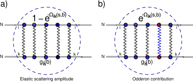
Figure 2: Shadowing corrections to the Odderon exchange: Fig. 2-a: elastic amplitude in the two channel model. Fig. 2-b: the shadowing corrections in our model. The wavy lines describe the Pomeron exchanges while the zigzag line corresponds to the exchange of the Odderon.

III.3 Numerical estimates

In this section we make estimates using our model for $\Omega$, with parameters that are given by Table I.

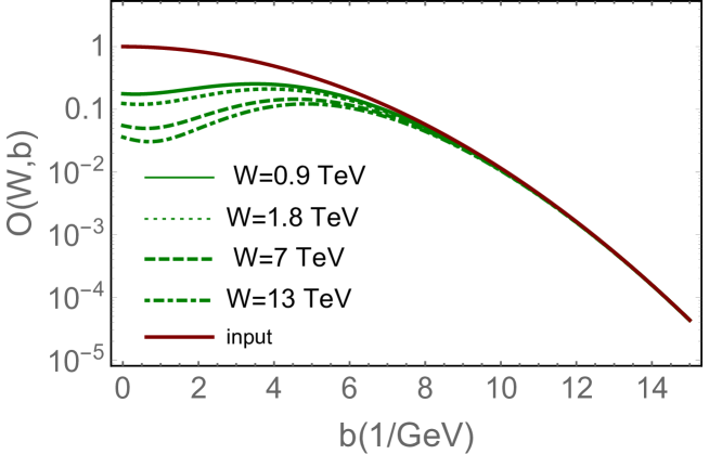
Figure 3: $O\left(W,b\right)$ versus $b$ for different energies. The red line corresponds to the contribution of Eq. (19).

In Fig. 3 we plot the $b$ dependence of the Odderon contribution. One can see that the shadowing corrections lead to a considerable suppression of the Odderon contribution at small $b$ in comparison with Eq. (19) (see red line in Fig. 3). This suppression is much smaller than in our approach, based on CGCGLP . The reason for this is that in our model the value of $A_{\rm el}\left(s,b\right)$ turns out to be smaller than 1 even at very high energies. Due to this $O\left(W,b=0\right)\,\,\neq\,\,0$ even at $W\approx 20TeV$.

In Fig. 4 we plot the contribution of the Odderon to the ratio of $\rho\,\,=\,\,{\rm Re}/{\rm Im}$ parts of the scattering amplitude as function of energy. One sees the influence of the shadowing corrections, which induce the energy dependence of this ratio on energy. Eq. (19) shows that the Odderon does not depend on energy without these corrections. This induced energy dependence turns out to be rather large causing a decrease of $\rho$ in the energy range: W = 0.5 $\div$ 20 TeV. However, this effect is much smaller than in our previous estimates GLP and the value of $\rho$ does not contradict the experimental data TOTEMRHO1 ; TOTEMRHO2 ; TOTEMRHO3 ; TOTEMRHO4 .

The shadowing correction has a remarkable effect on the $t$-dependence of the scattering amplitude (see Fig. 5 ). We see that the shadowing corrections lead to a narrower distribution over $t$, than the input given by Eq. (19), which is shown in Fig. 5 by the red line.

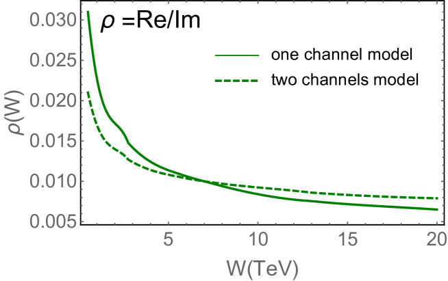
Figure 4: $\rho={\rm Re}/{\rm Im}$ due to the Odderon contribution versus W in our model. The solid line presents the estimates, using Eq. (21), while the dashed line describes the evaluation in two channel model of Ref.GLPPM2 .

$\Delta_{\rm dressed}$	$p_{0}$	$m(GeV)$	$\chi^{2}$/d.o.f
0.331 $\pm$ 0.030	0.483 $\pm$ 0.030	0.867 $\pm$ 0.005	1.3

Table 1: Fitted parameters.$\Delta_{\rm dressed}=\Delta\left(1-p_{0}\right)$.

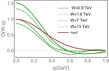
Figure 5: $O\left(W,q=\sqrt{|t|}\right)$ versus $q=\sqrt{|t|}$ for different energies. The red line corresponds to the contribution of Eq. (19).

IV Dependence of the elastic cross sections on $t$ and the Odderon

In this section we will look at another facet of the Odderon contribution: it could contribute to the real part of the scattering amplitude at the value of $t=t_{min}$, where $d\sigma_{\rm el}/dt$ has a minimum.

We attempt to describe the elastic cross section for $|t|=0\div 1\,GeV^{2}$ . Our model predicts the existence of a minimum in the elastic cross sections, however its position occurs at $|t|\,\approx\,0.3\,GeV^{2}$, which is much smaller than was observed experimentally by TOTEM collaborationTOTEMLT .

Assuming that this discrepancy is due to the simplified form of $b$ dependence of our amplitude which is given by Eq. (10), we changed the initial conditions of Eq. (10) to the following equations

$$p(b^{\prime})=p_{0i}\,S(b^{\prime},m,\mu,\kappa_{i})~{}~{}~{}\mbox{with}~{}~{}S(b,m,\mu,\kappa_{i})=\left(1-\kappa\right)\left(m\,b\right)^{\nu_{1}}K_{\nu_{1}}(m\,b)\,\,+\,\,\kappa\frac{\left(m\,b\right)^{\nu_{2}}K_{\nu_{2}}(\mu\,b)}{2^{\nu_{2}\,-\,1}\,\Gamma\left(\nu_{2}\right)}$$ (22)

In Table II we present the parameters that we found for the fit. Fig. 6 shows the comparison with TOTEM data of Ref.TOTEMLT . One can see that we obtain good agreement with the experimental data for $|t|\,<\,|t|_{min}$ and for $|t|\,>\,|t|_{min}$. However, for $|t|\approx\,|t|_{min}$ the real part of the scattering amplitude turns out to be small, and we obtain a value of the $d\sigma_{el}/d\,t$ approximately an order of magnitude smaller than the experimental one. It should be stressed that we do not use any of the simplified approaches to estimate the real part of the amplitude, but using our general expression of Eq. (17) for $A_{ik}\left(s,t\right)$, we consider the sum $A_{ik}\left(s,+i\epsilon t\right)+A_{ik}\left(u-i\epsilon,t\right)$, which corresponds to positive signature, and calculated the real part of this sum.

In Fig. 6 we estimate the contribution of the $\omega$ -reggeon , using the description taken from the paper of Ref.DOLA (note the difference between green dashed line and the blue solid curve). This contribution is small, and can be neglected.

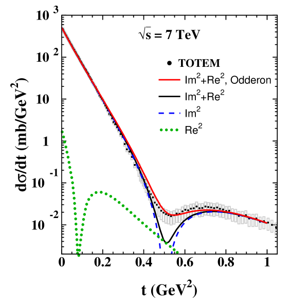
Figure 6: $d\sigma_{el}/dt$ versus $t$. The black green line describes the result of our fit. The dashed line corresponds to the contribution of the imaginary part of the scattering amplitude to the elastic cross section. The dotted line relates to the real part of our amplitude.The red solid line takes into account the contribution of the odderon to the real part of the $pp$ amplitude, as is shown in Eq. (25). The data , shown in grey, include systematic errors. They are taken from Ref.TOTEMLT .

To evaluate the real part of the amplitude we use the relation:

$${\rm Re}A_{11}(s,t)\,\,=\,\,\frac{1}{2}\,\pi\,\frac{\partial}{\partial\,\ln\left(s/s_{0}\right)}\,{\rm Im}A_{11}\left(s,t\right)|_{{Eq.~{}(\ref{AIK})}}$$ (23)

Eq. (23) correctly describes the real part of the amplitude only for small $\rho={\rm Re}A/{\rm Im}A$. In Fig. 7 we plot the $d\sigma/dt$ with these estimates for the real part. The real part from Eq. (23) turns out to be almost twice larger than the experimental data in the vicinity of $t_{min}$. Therefore, at the minimum, where ${\rm Im}\,A\,\ll\,{\rm Re}A$, Eq. (23) cannot be used for the real part. However, replacing Eq. (23) by

$${\rm Re}A_{11}(s,t)\,\,=\,\,\tan\left(\rho\right)\,{\rm Im}A_{11}\left(s,t\right)|_{{Eq.~{}(\ref{AIK})}}$$ (24)

we obtain the same result, that the real part of the amplitude turns out to be too large. Actually,Eq. (24) assumes that the scattering amplitude depends on energy as a power $A\left(s,t\right)\,\propto\,s^{2\,\rho/\pi}$. Our amplitude is a rather complex function of energy, and depends on $\ln(s)$.

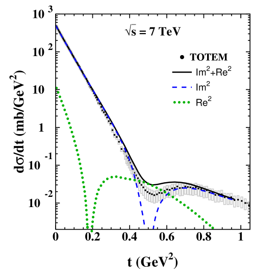
Figure 7: $d\sigma_{el}/dt$ versus $t$. The solid line describes the result of our fit. The dotted line corresponds to the contribution of the real part of the scattering amplitude to the elastic cross section, which is calculated using Eq. (23), with added contribution of the exchange of the $\omega$ - reggeon, which is taken from Ref.DOLA . We do not show the contribution of the real part without the $\omega$-reggeon as it coincides with the dotted line. The dashed line is the contribution of the imaginary part of the amplitude. The data are taken from Ref.TOTEMLT )

Variant of the fit	$\Delta_{\rm dressed}$	$p_{0}$	$m$ (GeV)	$\mu$(GeV)	$\nu_{1}$	$\nu_{2}$	$\kappa$
one channel model	0.48 $\pm$ 0.01	0.8 $\pm$ 0.05	0.860	7.6344	0.9	0.1	0.48

Table 2: Fitted parameters for $d\sigma_{el}/dt$ dependence.$\Delta_{\rm dressed}=\Delta\left(1-p_{01}\right)$.

Concluding, we see that to describe the TOTEM experimental data in the framework of our model, the contribution to the real part of the amplitude from the exchange of the odderonODD is needed. Hence, our estimates confirm the conclusions of Ref.ODDSC . In Fig. 6 we plot the description of the elastic cross section in which we have added the odderon contribution to the amplitude of Eq. (17) (red solid curve in Fig. 6):

$$f\left(s,t\right)\,\,=\,\,f\left(s,t;{Eq.~{}(\ref{AIK})}\right)\,\,\pm\,\,O(s,t)$$ (25)

where we consider a QCD odderonODD : the state with odd signature and with the intercept $\alpha_{\rm odd}(t=0)=1$, which contributes only to the real part of the scattering amplitude. $O(s,t)$ is given by Eq. (19). Our odderon parameters are in accord with the estimates in Ref.KMR . The amplitude $f(s,t)$ is related to $a_{el}\left(s,b\right)$ as

$$\frac{d\,\sigma_{el}}{dt}\,\,=\,\,\pi\,|f(s,t)|^{2};\,\,\,\,\,a_{el}(s,b)\,\,=\,\,\frac{1}{2\,\pi}\int d^{2}q\,e^{-i\boldsymbol{q}\cdot\boldsymbol{b}}\,f\left(s,t\right)\mbox{where}\,\,t\,=\,-q^{2}$$ (26)

In Fig. 8 we show the prediction for proton-antiproton scattering. One can conclude that in our model the measurements of the elastic cross sections for $p\,p$ and $\bar{p}p$ scattering can provide the estimates for the odderon contribution. It should be stressed that the contribution of the $\omega$-reggeon leads to negligible contribution at $W=7\,TeV$ (see Fig. 7).

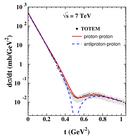
Figure 8: $d\sigma_{el}/dt$ versus $t$. The solid line describes the elastic cross sections for $pp$-scattering with the odderon contribution (see Eq. (25)), while the dashed line shows the elastic cross section for $\bar{p}p$-scattering using Eq. (25). The data are taken from Ref.TOTEMLT )

V Conclusions

In this paper we discussed the Odderon contribution in our modelGLPPM that provides a fairly good description of $\sigma_{\rm tot}$,$\sigma_{\rm el}$ and $B_{\rm el}$, especially as related to the energy dependence of these observables. We showed that the shadowing corrections are large and induce considerable dependence on energy for the Odderon contribution, which in perturbative QCD is energy independent . However, this energy dependence does not contradict the experimental data for $\rho={\rm Re}/{\rm Im}$, if we assume that the Odderon gives a contribution of about $1\div 4$ mb at W=7 TeV (see Fig. 9).

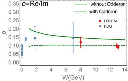
Figure 9: $\rho$ = Re/Im for proton-proton scattering versus $W=\sqrt{s}$. Data are taken from PDG PDG and from the TOTEM papers TOTEMRHO1 ; TOTEMRHO2 ; TOTEMRHO3 ; TOTEMRHO4 . The solid line shows the predictions of our model, while the dashed line presents the estimates for the value of $\rho$, adding the odderon contribution $4mb$ at W=13 TeV, to our model.

This fact is in striking contrast to our estimates for the CGC based modelGLP . The reason for this difference is that the elastic scattering amplitude in our eikonall model does not reach the unitarity limit ($A_{el}\left(W,b=0\right)=1$, even at very high energies. The contrast turns out to be more pronounced in the two channel modelGLPPM2 , which is shown by dashed lines in Fig. 4. However, we need to point out here that the comparison with the experimental data in the two channel model is worse than in the eikonal one, especially for $\sigma_{el}$.

Our attempt to describe the $t$-dependence of the elastic cross section shows that we can reproduce the main features of the $t$-dependence that are measured experimentally: the slope of the elastic cross section at small $t$, the existence of the minima in $t$-dependence which is located at $|t|_{min}=0.52\,GeV^{2}$ at W= 7 TeV; and the behaviour of the cross section at $|t|\,>\,|t|_{min}$.

It should be stressed that we do not use any of the simplified approaches to estimate the real part of the amplitude which we show ( in our model ), that they do not reproduce correctly the real part of the amplitude at large $t$. In our model the real part turns out to be much smaller than the experimental one. Consequently, to achieve a description of the data, it is necessary to add an odderon contribution. Hence, our model corroborates the conclusion of Ref.ODDSC .

Summarizing, in this paper we have presented estimates resulting from a simple eikonal model, which provides a fair description of the data on total and elastic cross sections. We are aware, that this is a simplified approach, which could be a good first approximation, but we need to go further. We plan to develop a model which will also describe diffraction production. We have made the first effort GLPPM2 , but we consider it as not very successful, and we need to continue our search. We also plan to re-visit our model based on CGC approach GLP , with the goal to improve it so that , we can also introduce the Odderon contribution. We believe that we can base these attempts on results for QCD Odderon KOLEB ; BLV ; KS ; LRRW ; YHH ; CLMS .

Acknowledgements.
We thank our colleagues at Tel Aviv University and UTFSM for encouraging discussions. Our special thanks go to Tamas Csörgő and Jan Kasper for discussion of the odderon contribution and elastic scattering during the Low x’2019 WS. This research was supported by CONICYT PIA/BASAL FB0821(Chile) and Fondecyt (Chile) grants 1170319 and 1180118 .

References

- (1) G. Antchev et al. [TOTEM Collaboration], “First measurement of elastic, inelastic and total cross-section at TeV by TOTEM and overview of cross-section data at LHC energies,” Eur. Phys. J. C 79 (2019) no.2, 103 doi:10.1140/epjc/s10052-019-6567-0 [arXiv:1712.06153 [hep-ex]].
- (2) G. Antchev et al. [TOTEM Collaboration], “First determination of the parameter at TeV: probing the existence of a colourless C-odd three-gluon compound state,” Eur. Phys. J. C 79 (2019) no.9, 785 doi:10.1140/epjc/s10052-019-7223-4 [arXiv:1812.04732 [hep-ex]].
- (3) G. Antchev et al. [TOTEM Collaboration], “Elastic differential cross-section measurement at TeV by TOTEM,” Eur. Phys. J. C 79 (2019) no.10, 861 doi:10.1140/epjc/s10052-019-7346-7 [arXiv:1812.08283 [hep-ex]].
- (4) G. Antchev et al. [TOTEM Collaboration], “Elastic differential cross-section at and implications on the existence of a colourless C-odd three-gluon compound state,” Eur. Phys. J. C 80 (2020) no.2, 91 doi:10.1140/epjc/s10052-020-7654-y [arXiv:1812.08610 [hep-ex]].
- (5) V. A. Khoze, A. D. Martin and M. G. Ryskin, “Elastic and diffractive scattering at the LHC,” Phys. Lett. B 784 (2018) 192 doi:10.1016/j.physletb.2018.07.054 [arXiv:1806.05970 [hep-ph]].
- (6) W. Broniowski, L. Jenkovszky, E. Ruiz Arriola and I. Szanyi, “Hollowness in and scattering in a Regge model,” arXiv:1806.04756 [hep-ph].
- (7) S. M. Troshin and N. E. Tyurin, “Implications of the measurements by TOTEM at the LHC,” arXiv:1805.05161 [hep-ph].
- (8) E. Martynov and B. Nicolescu, “Evidence for maximality of strong interactions from LHC forward data,” arXiv:1804.10139 [hep-ph].
- (9) M. Broilo, E. G. S. Luna and M. J. Menon, “Soft Pomerons and the Forward LHC Data,” Phys. Lett. B 781 (2018) 616, [arXiv:1803.07167 [hep-ph]].
- (10) Y. M. Shabelski and A. G. Shuvaev, ‘Real part of scattering amplitude in Additive Quark Model at LHC energies,” Eur. Phys. J. C 78 (2018) no.6, 497, [arXiv:1802.02812 [hep-ph]].
- (11) V. A. Khoze, A. D. Martin and M. G. Ryskin, “Black disk, maximal Odderon and unitarity,” Phys. Lett. B 780 (2018) 352, [arXiv:1801.07065 [hep-ph]].
- (12) V. A. Khoze, A. D. Martin and M. G. Ryskin, “Elastic proton-proton scattering at 13 TeV,” Phys. Rev. D 97 (2018) no.3, 034019, [arXiv:1712.00325 [hep-ph]].
- (13) E. Gotsman, E. Levin and I. Potashnikova, “CGC/saturation approach: secondary Reggeons and dependence on energy,” Phys. Lett. B 786 (2018) 472 doi:10.1016/j.physletb.2018.10.017 [arXiv:1807.06459 [hep-ph]].
- (14) T. Csörgő, T. Novak, R.Pasechnik, A. Ster and I. Szanyi, “Evidence of Odderon-exchange from scaling properties of elastic scattering at TeV energies,” arXiv:1912.11968 [hep-ph].
- (15) Yuri V Kovchegov and Eugene Levin, “ Quantum Choromodynamics at High Energies”, Cambridge Monographs on Particle Physics, Nuclear Physics and Cosmology, Cambridge University Press, 2012 .
- (16) J. Bartels, L. N. Lipatov and G. P. Vacca, “A New odderon solution in perturbative QCD,” Phys. Lett. B 477 (2000) 178, [hep-ph/9912423].
- (17) Y. V. Kovchegov, L. Szymanowski and S. Wallon, “Perturbative odderon in the dipole model,” Phys. Lett. B 586 (2004) 267, [hep-ph/0309281].
- (18) Carlos Contreras, Eugene Levin , Rodrigo Meneses and Michael Sanhueza,Non-linear equation in the re-summed next-to-leading order of perturbative QCD: the leading twist approximation,(in preparation).
- (19) E. Gotsman, E. Levin and I. Potashnikova, “A new parton model for the soft interactions at high energies,” Eur. Phys. J. C 79 (2019) no.3, 192, [arXiv:1812.09040 [hep-ph]].
- (20) A. Kovner, E. Levin and M. Lublinsky, “QCD unitarity constraints on Reggeon Field Theory,” JHEP 1608 (2016) 031, [arXiv:1605.03251 [hep-ph]].
- (21) T. Altinoluk, A. Kovner, E. Levin and M. Lublinsky, “Reggeon Field Theory for Large Pomeron Loops,” JHEP 1404 (2014) 075 [arXiv:1401.7431 [hep-ph]].
- (22) V. S. Fadin, E. A. Kuraev and L. N. Lipatov, “On the pomeranchuk singularity in asymptotically free theories”, Phys. Lett. B60, 50 (1975); E. A. Kuraev, L. N. Lipatov and V. S. Fadin, “The Pomeranchuk Singularity in Nonabelian Gauge Theories” Sov. Phys. JETP 45, 199 (1977), [Zh. Eksp. Teor. Fiz.72,377(1977)]; “The Pomeranchuk Singularity in Quantum Chromodynamics,” I. I. Balitsky and L. N. Lipatov, Sov. J. Nucl. Phys. 28, 822 (1978), [Yad. Fiz.28,1597(1978)].
-
(23)
M. Froissart, “Asymptotic Behavior and Subtractions in the Mandelstam Representation”, Phys. Rev. 123 (1961) 1053;
A. Martin, “Scattering Theory: Unitarity, Analitysity and Crossing.” Lecture Notes in Physics, Springer-Verlag, Berlin-Heidelberg-New-York, 1969. - (24) M. G. Ryskin, “Odderon and Polarization Phenomena in QCD,” Sov. J. Nucl. Phys. 46 (1987) 337 [Yad. Fiz. 46 (1987) 611].
- (25) E. M. Levin and M. G. Ryskin, “High-energy hadron collisions in QCD,” Phys. Rept. 189 (1990) 267.
- (26) The Review of Particle Physics (2018), M. Tanabashi et al. (Particle Data Group), Phys. Rev. D 98, 030001 (2018).
- (27) E. Gotsman, E. Levin and I. Potashnikova, “A new parton model for the soft interactions at high energies: two channel approximation,” [arXiv:1908.05673 [hep-ph]].
- (28) G. Antchev et al. [TOTEM Collaboration], “Measurement of proton-proton elastic scattering and total cross-section at = 7-TeV,” EPL 101 (2013) no.2, 21002. doi:10.1209/0295-5075/101/21002
- (29) V. A. Khoze, A. D. Martin and M. G. Ryskin, “Elastic and diffractive scattering at the LHC,” Phys. Lett. B 784, 192 (2018) doi:10.1016/j.physletb.2018.07.054 [arXiv:1806.05970 [hep-ph]].
- (30) A. Donnachie and P. V. Landshoff, “ and total cross sections and elastic scattering,” Phys. Lett. B 727 (2013) 500 Erratum: [Phys. Lett. B 750 (2015) 669] doi:10.1016/j.physletb.2015.09.017, 10.1016/j.physletb.2013.10.068 [arXiv:1309.1292 [hep-ph]].
- (31) J. Bartels, L. N. Lipatov and G. P. Vacca, “A New odderon solution in perturbative QCD,” Phys. Lett. B 477 (2000) 178 doi:10.1016/S0370-2693(00)00221-5 [hep-ph/9912423]; Y. V. Kovchegov, L. Szymanowski and S. Wallon, “Perturbative odderon in the dipole model,” Phys. Lett. B 586 (2004) 267 doi:10.1016/j.physletb.2004.02.036 [hep-ph/0309281].
- (32) T. Csörgő, T. Novak, R. Pasechnik, A. Ster and I. Szanyi, “Evidence of Odderon-exchange from scaling properties of elastic scattering at TeV energies,” arXiv:1912.11968 [hep-ph].
- (33) T. Lappi, A. Ramnath, K. Rummukainen and H. Weigert, “JIMWLK evolution of the odderon,” Phys. Rev. D 94 (2016) no.5, 054014 doi:10.1103/PhysRevD.94.054014 [arXiv:1606.00551 [hep-ph]].
- (34) X. Yao, Y. Hagiwara and Y. Hatta, “Computing the gluon Sivers function at small-,” Phys. Lett. B 790 (2019) 361 doi:10.1016/j.physletb.2019.01.029 [arXiv:1812.03959 [hep-ph]].
- (35) C. Contreras, E. Levin, R. Meneses and M. Sanhueza, [arXiv:2004.04445 [hep-ph]].